Optimization Model for the Integration of the Electric System and Gas Network: Peruvian Case

Abstract

This paper presents a method for multi-period optimization of natural gas and electric power systems incorporating gas-fired power plants to analyze the impact of the interdependence between those commodities, in terms of cost and energy supply. The proposed method considers electricity network constraints, such as voltage profile, electrical losses, and limits of the transmission lines, as well as the technical restrictions on the gas network, such as the diameter, length, pressure, and limits for those variables. The proposed method was applied to a 12-bus electric network and a 7-node gas network, and several interdependencies between the electricity and the natural gas system network can be observed. The results show how the restrictions cause the behavior of the gas-fired power plants—in a low demand stage, it is restricted even when the gas-fired power generation prices are below the hydraulic generation prices, while in scenarios of higher demand, saturated cargo flows are observed, causing bus bar prices to be affected with higher operating costs. In this sense, the results of the variation in bus bar prices show little price stability in some bus bars in different stages, due to the behavior of the generation supply that is forced to operate by system restrictions.

1. Introduction

The optimization problem, in regard to reducing the total cost of energy production in the short-term market, is challenging, due to the different energy sources, costs, and restrictions [1,2]. Likewise, these same energy sources depend on other variables and technical constraints, such as the variability of energy sources, technology constraints, and the inability to be manageable (solar and wind). Concerning natural gas (NG) plants, it will depend on the capacity of the sources, the transmission network, the restrictions of the same network [3], and efficient interactions between both networks [4]. This research describes the optimization model for economic dispatching of integrated electricity and natural gas systems based on the Peruvian national interconnected system (SEIN) and the Peruvian gas pipeline that arrives from Camisea to the Peruvian coast.

The interaction between the SEIN and the NG network was analyzed in an integrated way using an equivalent 12-bus electric system of the SEIN and the 7-node gas network, for a daily analysis period every sixty minutes; it included the costs of transportation, gas network restrictions, production costs of different energy sources, and electricity network restrictions operating simultaneously, through a mathematical model of discrete non-linear programming (DNLP), intending to define the simultaneous optimum of the NG network and the cost of operation of the energy systems. The 12-bus reduced equivalent system was developed by applying the non-linear ward equivalent method [5] of the SEIN network [6], obtained from the Council for Electrical System Economy Operating (COES).

There are a series of contributions related to the optimization models of the electricity markets [7,8] and NG [9] separately. On the other hand, literature on the modeling of integrated electricity–NG systems and the analysis of the behavior of the agents when they participate in the short-term market, is scarce. In the review, in [10], different approaches are grouped according to the time horizon for short-term market analysis.

Several authors have proposed models to analyze the electric and gas systems at the same time, especially to determine the planning of the systems considering aspects of stability and reliability, maximizing production with generators of combined cycle, through the reliability of the gas supply [11,12], while other authors minimize the total cost of electricity production subject to the limitations between gas and electricity networks [13], or the total cost of operation of an integrated gas–electricity system [14]. On the other hand, there are models (e,.g., in [15]) that maximize the welfare of all agents through the optimal set of gas and electricity flows. This social welfare is defined as the total benefits for electricity and gas consumers, with exception of the operations cost of the system.

For the real-time market in the gas networks, the gas flow—in order to be supplied to the natural gas electricity generators, as well as to other receivers that use said energy sources—depends on some variables, such as the pressure differences governing the gas flow [16] and gas demands that are calculated through a nodal gas balance [17]. The behavior of both variables adopts a method based on Benders decomposition.

In this sense, there is a large amount of literature, such as in [18], where the authors analyze integrated planning for gas and electric power transmission systems. In [19], where the expansion of the capacity problem considering both systems was presented. In [20], a long-term, multi-area, and multistage model for the supply/interconnection expansion planning of integrated electricity and natural gas (NG) was presented.

In the Peruvian case, the market and operation of the electric system and gas network are not integrated yet, so their optimization objectives are not dependent on each other. In addition to a series of inefficiencies already identified by the normative and regulatory agencies [10] and the market agents themselves, such as inefficient use of NG allocation, differences between contracted and consumed volumes, decreased NG well productivity due to the high percentage of NG reinjected to the reservoir, and the inefficient average cost of NG, are reflected in the variable fuel costs for determination of the marginal cost of generation of NG thermal power plants.

The main contributions of this paper can be summarized as follow:

1

Considerable simplification and unification of the equations of physical behavior of both networks (electric and gas networks) were realized, allowing to show the optimal production costs of the integrated gas–electricity model, the influence of restrictions on transmission, the gas pipeline network, the variation of bus prices of the electricity system, and the behavior of the network parameters.

2

The Peruvian integrated gas–electricity system was modeled, simulating the behavior of the short-term markets when the electricity and gas markets were coupling, through the application of discrete nonlinear programming.

3

An equivalent network of natural gas was explored, based on the information of the NG transportation pipelines from Camisea to Lima, with their respective parameters and restrictions; moreover, the 500 kV equivalent system of the electrical system of SEIN, obtained through the non-linear Ward equivalent method, was explored.

The paper is organized as follows. In Section 2, a description of the problem formulation identifying the objective function, electrical system, and natural gas equation is presented. In Section 3, the integrated modeling of natural gas and electric power networks is presented. In Section 4, the application and discussion of the proposed method are presented. In Section 5, the computer performance is presented. Conclusions and final considerations are presented in Section 6.

2. Problem Formulation

In the Peruvian case, the gas transmission network is taken into account and integrated into the simultaneous operation of the electrical network (the model could integrate more than one gas network). In this way, the thermoelectric plants connected to this network must decide the gas flow required for its operation, which will depend on the behavior of demand and the associated offers throughout the different nodes of the gas transportation network.

An optimization model was developed to solve the problem of the interconnected electric system and gas network for the Peruvian case. The amount of gas to be taken by the generators considering their storage capacity and the demand that it will be able to cover in multi-periods throughout the day [21], as well as the gas pipeline constraints and its interrelation with the operation of the electrical network [22], were considered.

2.1. Integrated Electricity–Gas Modeling

The objective function is defined by a mathematical model of discrete non-linear programming (DNLP) developed through programming in a general algebraic modeling system (GAMS), a tool that allows the formulation of complex optimization problems, such as the integrated operation of electrical and gas systems.

Operational optimization techniques have generally focused on a single energy transmission system under the assumption of an unrestricted supply for the different operators, which is why different methodologies have usually been developed separately, both for the electricity market and natural gas [8]. Other approaches have recently been presented that address the integrated modeling and analysis of electricity–gas energy systems in a more comprehensive and generalized way. These approaches consider multiple energy carriers, so, for our case, we define an optimization function based on energy production costs plus the costs of transporting gas from its source along with the gas pipeline system.

Both systems include integer variables with nonlinear constraints and assumptions, defined as follows:

• The system must maintain a balance of its energy flow;
• Individual generator restrictions (including dispatch price, generation limits, etc.);
• Power transmission constraints;
• NG source limits and NG transportation constraints;
• Coupling of the electrical and gas system;
• Hydrogenerating units are considered as a linear cost function;
• The flow integration period t will be one hour for an analysis of 24-h.

2.1.1. Objective Function

The objective function (FO) is defined by the operational costs of electric energy (EC) dispatched by each thermal unit plus the cost of natural gas (GC) dispatched (and/or imported) added to the costs of gas transportation (TC), along with the gas pipeline system, so the function involves not only energy production costs but also the costs involved in transporting gas and doing it efficiently. Transmission costs are not included in the objective function, since these costs are distributed proportionally among the energy suppliers of the SEIN.

$$FO=EC+GC+TC$$

(1)

$$EC=\sum _{g=1}^{Gen}\sum _{t=1}^{24}(b_g*P_g^2\left(t\right)+a_g*P_g\left(t\right)+c_g)$$

(2)

$$GC=\sum _{n=1}^{NGs}\sum _{t=1}^{24}(S_n\left(t\right)*p_{ng})$$

(3)

$$TC=\sum _{l=1}^{PG}\sum _{t=1}^{24}(f_{nm}\left(t\right)*p_{tg})$$

(4)

where:

$P_g\left(t\right)$: active power generation from generator g in the period t in [MW].

$b_g,a_g,and{c}_g$: are the cost co-efficients of unit g, as a function of the generator power in units [$/MW2], [$/MW], and [$], respectively.

$S_n$: supply of natural gas dispatched or imported at node n in period t in [106 m${}^3$/h].

$P_{ng}$: price of natural gas in [$/m${}^3$].

$f_{nm}\left(t\right)$: flow between nodes n and m in period t in [106 m${}^3$/h].

$p_{tg}:$ natural gas transportation cost in [$/m${}^3$].

$PG$: number of pipeline gas.

$NGs$: number of natural gas supplies in the gas system.

$Gen$: number of generators in the electrical system.

2.1.2. Electrical System

The power flow equations are defined by the product of the impedance of the network and the potential difference in its polar form, both for the active power $P_i$ and the reactive power $Q_i$ for a typical bus i.

(a)

Power flow:

$$P_i=\sum _{j=1}^N\left|Y_{ij}{V}_i{V}_j\right|cos\left({\theta }_{ij}+{\delta }_j-{\delta }_i\right)\forall t$$

(5)

$$Q_i=-\sum _{j=1}^N\left|Y_{ij}{V}_i{V}_j\right|sin\left({\theta }_{ij}+{\delta }_j-{\delta }_i\right)\forall t$$

(6)

Notation:

$$Y_{ij}=\left|Y_{ij}\right|〈{\theta }_{ij}=\left|Y_{ij}\right|cos{\theta }_{ij}+j\left|Y_{ij}\right|sin{\theta }_{ij}=G_{ij}+j{B}_{ij}$$

(7)

$$V_i=\left|V_i\right|〈{\delta }_i=\left|V_i\right|(cos{\delta }_i+jsin{\delta }_i)$$

(8)

$$-P_{km}^{max}\le P_{km}\le P_{km}^{max}$$

(9)

where:

$P_i$: active power generated at bus i;

$Q_i$: reactive power generated at bus i;

$Y_{ij}$: total impedance of the line between bus i and bus j;

${\theta }_{ij}$: angle of the total admittance of the line between bus i and bus j;

${\delta }_i$: angle of voltage at bus i;

$P_{km}^{max}$: upper limit of active power through the line k-m (MW);

$P_{km}$: active power through the line k-m (MW).

(b)

Losses in the electrical system:

$$P_L=\sum _{i=1}^N{P}_{gi,t}-\sum _{i=1}^N{P}_{di,t}\forall t$$

(10)

$$Q_L=\sum _{i=1}^N{Q}_{gi,t}-\sum _{i=1}^N{Q}_{di,t}\forall t$$

(11)

where:

$P_L$: represents the total active power losses in period t;

$Q_L$: represents the total reactive power losses in period t;

${\sum }_{i=1}^N{P}_{gi,t}$: represents the total generation at bus i in period t;

${\sum }_{i=1}^N{P}_{di,t}$: represents the total active load at bus i in period t;

${\sum }_{i=1}^N{Q}_{gi,t}$: represents the total reactive generation at bus i in period t;

${\sum }_{i=1}^N{Q}_{di,t}$: represents the total reactive load at bus i in period t;

N: number of buses in the electric system.

(c)

Power balance:

$$\sum _{g=1}^G{P}_{gi,t}-P_{di,t}=\sum _{j=1}^N\left|Y_{ij}{V}_{i,t}{V}_{j,t}\right|cos\left({\theta }_{ij}+{\delta }_{j,t}-{\delta }_{i,t}\right)\dots \dots \forall i,t$$

(12)

$$\sum _{g=1}^G{Q}_{gi,t}-Q_{di,t}=-\sum _{j=1}^N\left|Y_{ij}{V}_{i,t}{V}_{j,t}\right|sin\left({\theta }_{ij}+{\delta }_{j,t}-{\delta }_{i,t}\right)\dots \dots \forall i,t$$

(13)

$$V_{min}\le V_{i,t}\le V_{max}\dots \dots \forall i,t$$

(14)

$${\delta }_{min}\le {\delta }_{i,t}\le {\delta }_{max}\dots \dots \forall i,t$$

(15)

where:

${\sum }_{g=1}^G{P}_{gi,t}$: represents the total active power of the generators connected at bus i in period t;

${\sum }_{g=1}^G{Q}_{gi,t}$: represents the total reactive power of the generators connected at bus i in period t;

$P_{di,t}$: represents the active load at bus i in period t;

$Q_{di,t}$: represents the reactive load at bus i in period t;

The units are represented in p.u. values, to be transformed into units; active power is in MW and reactive power in MVA.

2.1.3. Natural Gas System

(a)

Energy production equations of Natural Gas-Fueled Thermoelectric Power Units (NGFTPUs):

If we define a pipeline network where there are some nodes with a specific demand of $NG$ for use in electricity generation, the following equations [12] would be presented for the $NGFTPUs$:

$$P_{gi,min}\le P_{gi,t}\le P_{gi,max}\dots \dots \forall i,t$$

(16)

$$\sum _{n=1}^{NGs}{P}_{gi}\left(e_n\right)=P_{di}\dots \dots \forall t$$

(17)

$$P_{gi}=\eta \left(e_n\right)*LHV*e_n$$

(18)

where:

$P_{gi}$: power generated in MW by the combined cycle at bus i

$e_n$: the flow of NG towards the generator in m${}^3$/s from node n;

$\eta$: the efficiency of the combined cycle plant;

$LHV$: low heating value, with a value of 35.07 MW/( m${}^3$/s).

Equation (16) shows us the limits of the generation power of the NGFTPUs located at node n. In most NGFTPUs, the value of the minimum generation power is different from zero; to operate stably, a minimum generation power or a minimum operating flow is required.

Equation (17) represents the total demand for electrical power $P_{gi}$ required by the system with thermal generation at NG. These NGFTPUs are integrated into the high voltage transmission system, so the power offered by each NGFTPU will depend on the system’s demand for this resource or technology and the capacity of the NG network to deliver NG to meet said demand. This is the objective of the minimum cost of generation, production, and transportation of NG throughout the integrated system.

Equation (18) describes the relationship between the production of electrical energy generated by a combined cycle of NGFTPUs and the amount of NG it receives.

Equation (16) shows us the limits of the generation power of the NGFTPUs located at node n. Ultimately, this relationship of energy production and NG flow is not linear since it depends on the characteristics of the combined cycle plant, characteristics of the NG itself, and factors inherent to the location of the plant, such as altitude (in msnm), the climate (temperature, relative humidity, etc.) [12]; then the energy production in a combined cycle plant is a cubic function of the flow of NG e, so the previous function can be formulated with the following equation.

$$P_{gi}\left(e_n\right)=k_3{e}_n^3+k_2{e}_n^2+k_1{e}_n$$

(19)

where $k_3,k_2,$ and $k_1$ are coefficients that depend on the characteristics of the combined cycle NG thermal generation plant. Since obtaining the coefficients is complicated; Refs. [12,22] have used a simplification to Equation (19), shown for the test networks of this research work, in such a way that, for each power unit in MW produced, the approximation of the necessary $NG$ is 0.05 m${}^3$/s or 4320 m${}^3$/day of $NG$; that is:

$$P_{gi}\left(e_n\right)=k_1*e_n$$

(20)

where:

$k_1$ = 0.0023148 MW.day/106 m${}^3$

(b)

NG flow equations:

As indicated in numeral IV, the equivalent model of a NG network is composed of nodes where NG is injected or withdrawn, where the material balance must be fulfilled in each node, where the flows from the production or import of NG that enter to the node are equivalent to the NG flows for electrical and non-electrical generation purposes and the flows that are transported to other nodes [12].

$$S_n+\sum _m{f}_{mn}=\sum _j{f}_{no}+d_n+e_n\forall t$$

(21)

where:

$S_n$: NG supply at node n from production or import (m${}^3$/h o m${}^3$/día);

$f_{mn}$: NG flow from node m to node n (m${}^3$/h o m${}^3$/día);

$f_{no}$: NG flow from node n to node o (m${}^3$/h o m${}^3$/día);

$e_n$: NG demand at node n for electrical use (m${}^3$/h o m${}^3$/día);

$d_n$: NG demand at node n for non-electrical use (m${}^3$/h o m${}^3$/día).

In this way, Equation (21) responds to the application of the NG flow balance at node n; however, these flows will depend on other characteristics associated with NG, such as the pressure of the NG at the entrance and exit of the node, the section of the pipe, where the Weymouth Equation (22) must be fulfilled, an equation that responds to the quadratic relationship between the pressures and the NG flow.

$$Sign\left(f_{nm}\right){f_{nm}}^2={C_{nm}}^2(p_n^2-p_m^2)\forall t$$

(22)

$${f_{nm}}^2\le {{-C}_{nm}}^2(p_n^2-p_m^2)\forall t$$

(23)

$$p_{n,min}\le p_n\le p_{n,max}\forall t$$

(24)

$$f_{nm,min}\le f_n\le f_{nm,max}\forall t$$

(25)

$$S_{n,min}\le S_n\le S_{n,max}\forall t$$

(26)

where:

$p_n$: pressure at node n (bars);

$p_m$: pressure at node m (bars);

$C_{nm}^2$: constant that depends on the composition of the NG, on the length, diameter, and roughness of the nm section of the gas pipeline network (m${}^6$/bars${}^2$).

Subject to the following restrictions:

$f_{nm,max}$: upper limit of the NG flow from node n to node m, (m${}^3$/h);

$f_{nm,min}$: lower limit of the NG flow from node n to node m, (m${}^3$/h);

$p_{n,max}$: upper limit of the pressure at node n, (bars);

$p_{n,min}$: lower limit of pressure at node n, (bars);

$S_{n,max}$: upper limit of NG supply delivered by the producer or importer node n (m${}^3$/h);

$S_{n,min}$: lower limit of NG supply delivered by producer or importer node n (m${}^3$/h)

As can be seen, $C_{nm}$ is a constant that depends on the properties of the NG pipe (length, diameter, and absolute roughness) and the composition of the NG.

It is important to note that the flow is not restricted in the sign, if $f_{nm}>0$, the NG flows from node n to node m, and if $f_{nm}<0$ flows from node m to node n. In Equation (23), we have the flow of NG in an active pipe, it is also a quadratic function of the pressures at the end nodes. In this case, the inlet pressure at node n is less than the pressure at outlet node m ($p_n>p_m$) and the NG flows from node n to node m ($f_{nm}>0$).

Equation (23) represents a restriction related to active nodes; that is, with compressors. The compressors are equipment responsible for increasing the pressure at points where the NG needs to be at a higher pressure, guaranteeing a greater flow than is allowed in a gas pipeline or forcing NG paths in the network; for example, in the Peruvian case, it requires increasing the pressure of the NG to pass the flows to the other side of the Andes mountain range. In summary, in the results of the case studies, the compressors will ignore a maximum flow restriction and force a greater volume of NG into gas pipeline transmission networks, but with the pressures remaining within their limits.

Similarly, for restriction (26), corresponding to the delivered NG supply Sn, the same flow dynamics follows. If $Sn>0$ at node n, then this node is a producer or importer node of NG. If $Sn<0$ at node n, then the node is a consumer of NG, without ruling out electrical or non-electrical purposes.

The function $Sign\left(f\right)$ contained in Equation (22) collects the flow signal, thus defining its meaning:

$$Sign\left(x\right)=\left\{\begin{array}{c}0,ifx=0\\ 1,ifx>0\\ -1,ifx<0\end{array}\right.$$

(27)

For example, if a flow from node m to node n is defined as positive, the result after the simulation is in that sense if $fmn>0$. Otherwise, if the simulation result gives $fmn<0$, then the NG flows through the pipeline in the direction of n to m. A sign function avoids declaring the same gas pipeline twice for the program.

Inequality (25) refers to the physical restrictions of the gas pipelines. They are the maximum and minimum limits of NG flow in a gas pipeline that starts from node m to node n. Generally, the lower limit is zero, but if there are compressors in the gas pipeline, it may be that there is a minimum flow different from zero. The maximum flow can be calculated by:

$$f_{nm}=\sqrt{C_{nm}^2(p_n^2-p_m^2)}$$

(28)

where, $f_{nm}>0$, the flow of NG goes from node i to node j$f_{nm}<0$, the flow of NG goes from node j to node i. This term introduces a binary variable into the model and turns the formulation into a combinatorial problem.

Each constant $C_{nm}$ present in Equations (29) and (30) can be expressed as follows:

$$C_{nm}=96.074830*{10}^{-15}\frac{D_{nm}^5}{{\lambda }_{nm}*z*T*L_{nm}\delta }$$

(29)

$$\frac{1}{{\lambda }_{nm}}=9{\left[2log\left(\frac{3.7D_{nm}}{\epsilon }\right)\right]}^2$$

(30)

where:

$D^{nm}$: Internal diameter of the gas pipeline (mm);

z: NG compressibility factor, 0.8 (dimensionless);

T: NG temperature, 281.15 K;

$Lnm$: length of the gas pipeline nm (km);

$\delta$: density of NG relative to air, 0.6106 (dimensionless) and;

$\epsilon$: absolute roughness of the gas pipeline, 0.05 mm.

3. Integrated Modeling of Natural Gas and Electric Power Networks

3.1. Electrical System Model

A reduced equivalent circuit was developed at the 500 kV network level of the SEIN through the philosophy of the “Non-Linear Ward Equivalent” [5], starting from the parameters of the SEIN system with constant current injections, obtaining a relationship among the injected currents, the nodal voltage, and the nodal admittance, obtaining the injected currents as a function of the equivalent nodal admittance, separating into:

• A linear part, composed of equivalent admittance between nodes of the internal system and equivalent elements in derivation between these nodes and the common reference.
• A non-linear part, formed by equivalent injections in the nodes of the internal system.

(a)

Non-linear Ward equivalent in SEIN, application:

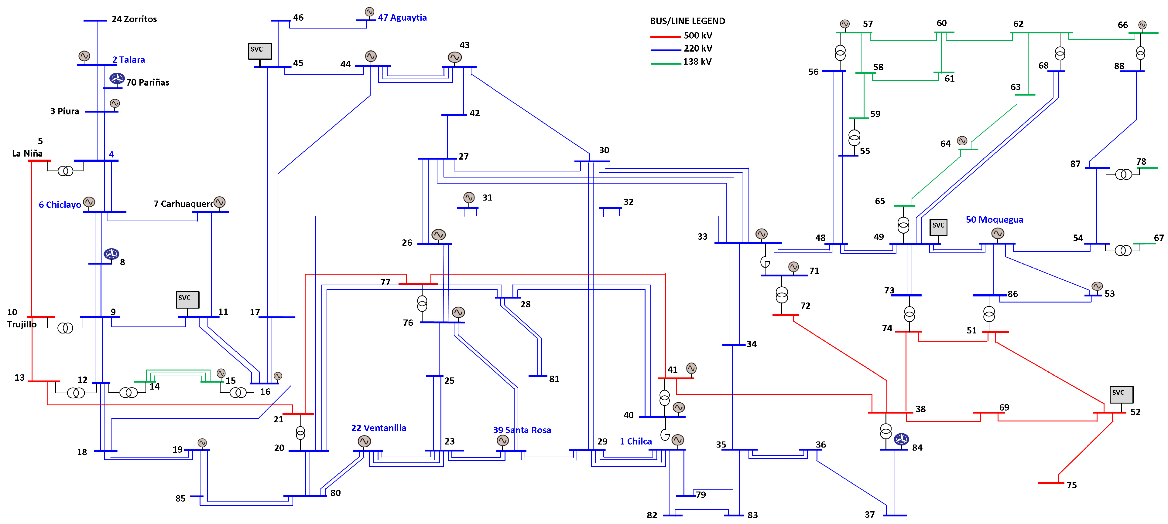
A non-linear Ward equivalent model was elaborated at the 500 kV network level of the SEIN for the flood period of the year 2020 (reduced equivalent model), under the method of “non-linear Ward equivalent” on the current electrical model of the SEIN, the same which presents 88 nodes at voltage levels of 500, 220, and 138 kV, loads modeled on 63 system nodes with a total demand of 6273.4 MW and 3252.9 MVAR. The information on electrical parameters and topology comes from the reference network of the electrical model and is obtained from the “Daily maintenance program” of COES [6] available for Power Factory DIgSilent program (see Figure 1).

The typical dispatches of the generation plants were determined to meet the balance with the demand of the loads and losses of the system; they were obtained from the energy model available in the stochastic dual dynamic programming (SDDP) program for the period 2020–2023 [23].

The database with the information on the electrical model of the SEIN operation for the year 2020 was stored in the IEEE CDF (common data format) [24], which allows power flow executions.

(b)

Non-linear reduced equivalent model of SEIN at the 500 kV.

Based on the current 88-bus electrical model of the SEIN, a non-linear reduced equivalent model of 500 kV was obtained for the period of 2020, which complies with the following aspects:

• The reduced equivalent model obtained is similar in topology to the electrical network of the current 88-bus SEIN electrical model. This model includes the electrical parameters of the impedances between the 500 kV nodes of the equivalent system, keeping the bus parameters corresponding to the 500 kV nodes reduced in the equivalent model.
• The reduced equivalent model obtained includes the load parameters in the 500 kV nodes with a demand equal to the power injections obtained in the non-linear reduced equivalent of the SEIN. Therefore, the loads and generation plants not included in the 500 kV nodes are transferred in active and reactive power through the non-linear reduced equivalent to the 500 kV nodes.

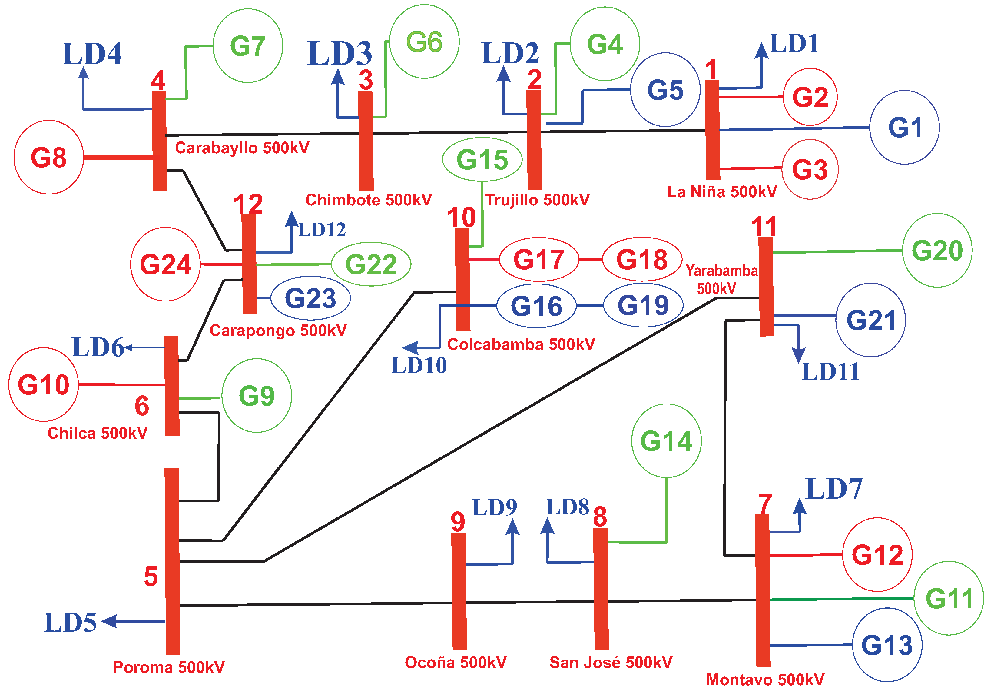
Figure 2 shows the one-line diagram of the reduced non-linear equivalent model of SEIN at the 500 kV network level for the year 2020, which presents 12 nodes of 500 kV.

The reduced model is formed by the elements of the admittance matrix (in p.u.) of the reduced equivalent network.

Table 1. Transmission line data of the reduced equivalent model in 500 kV (12-bus) of the SEIN.

Name Line (500 kV)	From	To	Admittance (p.u)	PHI (${}^{\circ }$)	R (p.u)	X (p.u)	LIMIT (MW)
LT La Niña-Trujillo	1	2	28.33	−1.49	0.0027	0.0352	420.3
LT Trujillo-Chimbote	2	3	62.38	−1.51	0.001	0.016	438.6
LT Chimbote-Carabayllo	3	4	23.15	−1.5	0.003	0.0431	376.6
LT Carabayllo-Carapongo	4	12	292.1	−1.45	0.0004	0.0034	1379.7
LT Carapongo-ChilcaCTM	12	6	129.34	−1.48	0.0007	0.0077	780
LT Chilca-Poroma	6	5	20.99	−1.49	0.0037	0.0475	646.3
LT Poroma-Ocoña	5	9	71.51	−1.37	0.0028	0.0137	491
LT Ocoña-San José	9	8	140.08	−1.37	0.0014	0.007	267.5
LT Montalvo-Yarabamba	7	11	76.16	−1.5	0.0009	0.0131	584.2
LT Poroma-Colcabamba	5	10	47.42	−1.44	0.0028	0.0209	889.2

shows the series elements, admittance, and impedance (in p.u.), of the electrical model reduced by 500 kV (12 bus) of the SEIN. The generators are also associated with the equivalent system.

Table 2. Generator data of the equivalent model in 500 kV of the SEIN.

Gen	Complete Name	Bus	Unitary Cost ($/MW)	Pmax (MW)	Pmin (MW)	Qmax (Mvar)	Qmin (Mvar)	Source
G1	La Nina 500 kV	B1	80.65	17.55	5.00	3.51	1.00	Residual
G2	La Nina 500 kV	B1	8.60	233.84	135.60	111.84	29.86	Natural Gas
G3	La Nina 500 kV	B1	41.82	51.28	25.60	10.26	5.12	Natural Gas
G4	Trujillo 500 kV	B2	50.21	149.04	20.58	29.48	0.07	hydraulic
G5	Trujillo 500 kV	B2	217.35	405.59	125.85	86.63	11.29	Diesel
G6	Chimbote 500 kV	B3	50.21	389.78	44.13	93.81	0.30	hydraulic
G7	Carabayllo 500 kV	B4	50.21	322.82	35.22	75.45	0.42	hydraulic
G8	Carabayllo 500 kV	B4	8.93	497.82	291.54	99.56	58.31	Natural Gas
G9	ChilcaCTM 500 kV	B6	50.21	242.45	24.82	52.00	0.02	hydraulic
G10	ChilcaCTM 500 kV	B6	8.52	2 845.24	1 559.00	569.05	311.80	Natural Gas
G11	Montalvo 500 kV	B7	50.21	151.19	22.77	29.29	0.03	hydraulic
G12	Montalvo 500 kV	B7	51.28	140.34	88.00	20.00	0.02	Coal
G13	Montalvo 500 kV	B7	196.99	1.152.80	623.24	226.88	123.91	Diesel
G14	San Jose 500 kV	B8	191.43	708.27	368.00	141.65	73.60	Diesel
G15	Colcabamba 500 kV	B10	50.21	2 214.82	382.67	608.56	78.88	hydraulic
G16	Colcabamba 500 kV	B10	207.33	89.50	10.42	27.53	2.08	Diesel
G17	Colcabamba 500 kV	B10	11.14	176.05	120.00	35.21	24.00	Natural Gas
G18	Colcabamba 500 kV	B10	32.46	91.03	64.50	18.21	12.90	Natural Gas
G19	Colcabamba 500 kV	B10	195.58	56.71	31.00	11.34	6.20	Residual
G20	Yarabamba 500 kV	B11	50.21	455.58	54.33	173.62	44.06	hydraulic
G21	Yarabamba 500 kV	B11	228.19	45.80	22.32	9.16	4.46	Diesel
G22	Carapongo 500 kV	B12	50.21	931.19	210.54	261.89	34.79	hydraulic
G23	Carapongo 500 kV	B12	206.40	211.46	125.00	42.29	25.00	hydraulic
G24	Carapongo 500 kV	B12	17.60	187.79	133.00	37.56	26.60	Natural Gas

describes the generator’s data associated with the buses of the equivalent system, and

Table 3. Results of power flow execution (AC model) applied to the non-linear reduced equivalent model in 500 kV (12-bus) of the SEIN.

Bus	Name Bus	Final Voltage, p.u.	Final Angle	Load MW	Load MVAR	Gen. MW	Gen. MVAR	Base KV
B1	La Nina 500 kV	1.000	−40.16	420.3	230	96.3	32.7	500
B2	Trujillo 500 kV	1.000	−33.54	438.6	224.7	30.3	39.5	500
B3	Chimbote 500 kV	1.000	−26.73	376.6	87.1	333.5	167.8	500
B4	Carabayllo 500 kV	1.000	−6.63	1379.7	900.5	908.6	643.6	500
B5	Poroma 500 kV	0.969	−7.39	780	101.7	0	0	500
B6	Chilca 500 kV	1.000	0	646.3	517.3	1841	735.5	500
B7	Montalvo 50 0kV	1.000	−10.49	491	268.6	167	150.7	500
B8	San Jose 500 kV	0.999	−10.67	267.5	70.5	0	316	500
B9	Ocoña 500 kV	0.986	−9.60	0	−96.8	0	0	500
B10	Colcabamba 500 kV	1.000	−1.74	584.2	452.5	1332.6	307.6	500
B11	Yarabamba 500 kV	1.000	−7.64	0	−150	383	167	500
B12	Carapongo 500 kV	1.000	−4.11	889.2	646.8	1251.3	−1.3	500

shows the results of the power flow applied to the reduced equivalent model in 500 kV (12-bus).

3.2. Gas System Model

An equivalent model of the NG pipeline network has been determined, allowing simulations of its behavior to be carried out.

(a)

Equivalent model of a non-linear natural gas network:

An equivalent model of the NG network was developed that contains the parameters of the network, allowing the problem of the distribution of NG through a pipe network subject to non-linear flow pressure relationships, material balances, and limits of pressure [25].

The NG network consists of several supply points (nodes) (sources of entry of NG or imported NG) or NG withdrawal (for electrical and non-electrical use), the pipes are represented as NG lines (passive) that are joined between nodes, where the compression systems of NG (active lines) [26] can be reflected in such a way that the interaction in a node of the NG network can be expressed as follows:

$f_{mn}$: Flow from node n to m (m${}^3$/h or m${}^3$/day);

$S_n$: $NG$ supply at node n from production or import (m${}^3$/h or m${}^3$/day);

$e_n$: $NG$ demand at node n for electrical use (m${}^3$/h or m${}^3$/day);

$d_n$: $NG$ demand at node n for Non-electric use (m${}^3$/h or m${}^3$/day).

(b)

Equivalent model of the Peruvian gas pipeline network.

The NG extracted from the fields of Block 88, San Martín, and Cashiriari, Department of Cusco, is the longest gas pipeline currently operated in Peru, having as its main function, transporting NG from the treatment plant in Malvinas, (Figure 3), crossing the Peruvian Andes to the coast of the Department of Lima, with a total length of the gas pipeline of 729 km.

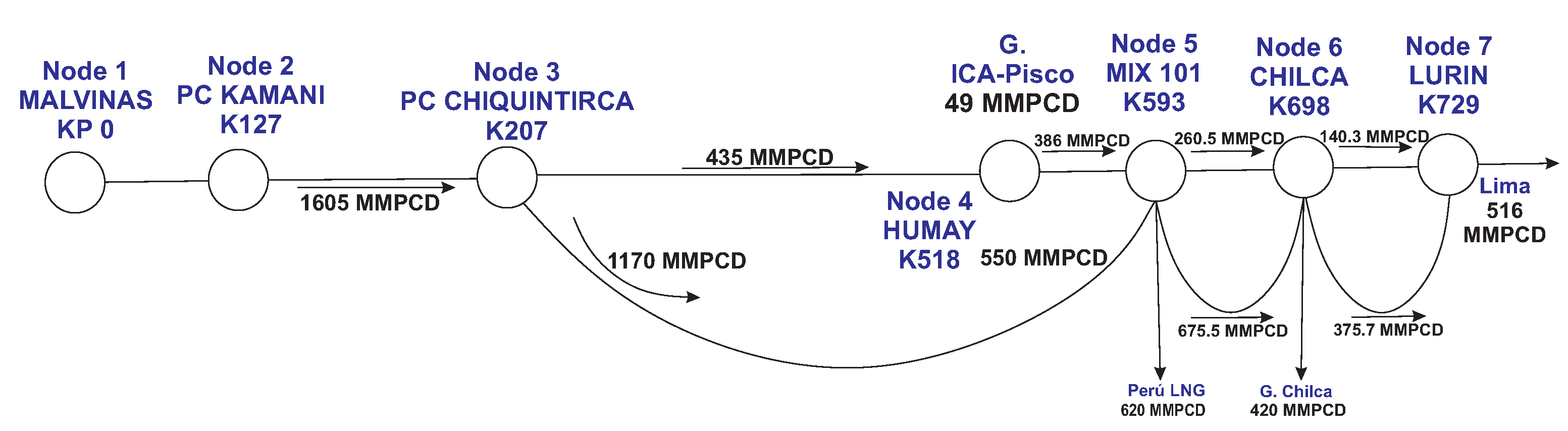
The transportation system is made up of a “14 and 10” diameter pipeline of approximately 557 km in length, from Malvina (KP0) to Pisco. Figure 4 shows the transportation capacity diagram of the Peruvian gas pipeline.

The gas network has seven nodes starting in Las Malvinas (Node 1), passing through Kamani (Node 12) and Chiquintirca (Node 3), which are the nodes that require compression to break the inertia of the elevation difference when passing through the Peruvian Andes. Before reaching Humay (Node 4), there is a network bypass with an NG outlet to Ayacucho, which currently has no NG consumption that is destined for future projects. The pipeline continues to Pampa Melchorita, called Mix 101 (Node 5) sends NG to the Peru liquefied natural gas (LNG) plant, then passes through Chilca (Node 6) with its derivation for the supply of NG from the NGFTPUs, finally reaching Lurín (Node 7), where the NG is sent to Lima for electrical and non-electrical use. Figure 5 shows the diagram of the gas pipeline transport capacities, as well as the location of its nodes; additionally, in

Table 4. Reference points of the natural gas transportation company of Peru (from https://observatorio.osinergmin.gob.pe/ accessed on 3 February 2022).

Node		KP	Zone	North	East
Node 1	Malvinas	KP 0	18	8,689,907.55	724,013.26
Node 2	Kamani	KP 127	18	8,599,403.00	691,070.00
Node 3	Chiquintirca	KP 207	18	8,599,333.00	691,017.00
Node 4	Humay	KP 517.9	18	8,480,890.00	404,048.00
Node 5	Mix 101 (CUA)	KP 594.9	18	8,536,618.00	361,063.00
Node 6	Chilca	KP 699	18	8,614,339.00	314,286.00
Node 7	Lurín	KP 729	18	8,640,336.00	300,970.00

, the distance between nodes and their geographical coordinates can be observed.

Table 5. Lengths of the main network, including the diameter of the pipeline (adapted from Osinergmin [27]).

Line	Start Node	End Node	Compressor	Diameter (Inch)	Length (km)
L1	Node 1 (Malvinas)	Node 2 (Kamani)	SI	32	126.7
L2	Node 2 (Kamani)	Node 3 (Chiquintirca)	SI	32	81.27
L3	Node 3 (Chiquintirca)	Node 4 (Humay)	NO	24	309.93
L4	Node 4 (Humay)	Node 5 (Mix 101)	NO	18	75.24
L5	Node 3 (Chiquintirca)	Node 5 (Mix 101)	NO	34	406
L6	Node 5 (Mix 101)	Node 6 (Chilca)	NO	18	105
L7	Node 5 (Mix 101)	Node 6 (Chilca)	NO	24	105
L8	Node 6 (Chilca)	Node 7 (Lurín)	NO	18	31.16
L9	Node 6 (Chilca)	Node 7 (Lurín)	NO	24	31.16

shows the lengths of the main pipeline by section and pipe diameter, including the network that belongs to other operators, such as Peru LNG and the Loop Coast. Maximum and minimum flows considering electric and non-electric demands are presented in

Table 6. Maximum and minimum flows considering electric and non-electric demands (adapted from Osinergmin) [27].

Node	Production Level		Use (Max)		Pressure Levels
	Min	Max	Elect	No Elect	Min (bar)	Max (bar)
	MMPCD	MMPCD	MMPCD	MMPCD
1	460	1605	0	0	147	147
2	460	1605	0	0	136	147
3	225	435	0	0	109	147
4	196	386	49	0	120	135
5	416	936	0	620	113	102
6	203	516	420	0	104	54
7	203	516	0	516	104	46

.

4. Application of the Proposed Method and Results

As defined in Section 3, the proposed optimization model analyzes the operation of the electrical system and the NG network in an integrated manner, in periods of one hour, in search of the lowest cost of operation, considering fuel costs of NG generating units, and the energy production costs of other technologies, the system losses and the restrictions of each of the systems, such as power balances, the generator constraints (including dispatch price, generation limits, etc.), power transmission constraints; the limits of sources of NG, the transport constraints of NG, and the coupling of the electricity and gas system.

The equations are defined as a mixed nonlinear optimization problem, where the difficulty in solving is found in Equations (19) and (20) due to the binary terms and the nonlinear relationships and restrictions defined in the proposed model.

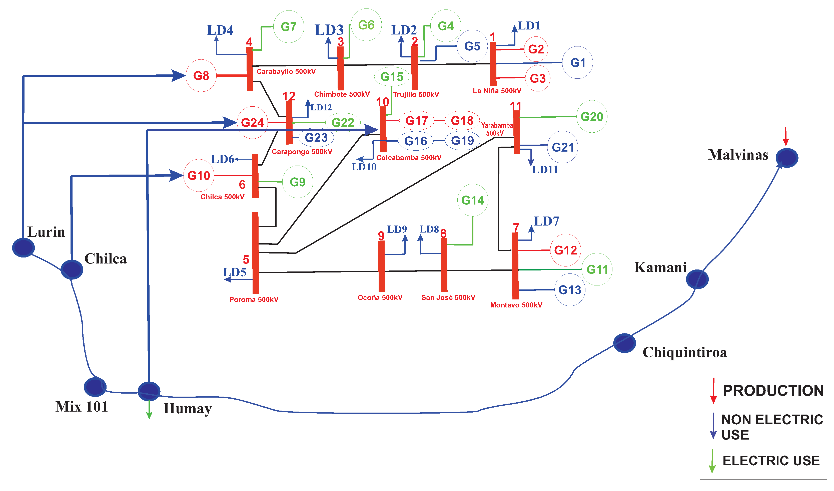
In this section, the simulation results are presented in order to analyze the different case studies carried out; Figure 6 shows the Diagram of the Peruvian gas–electricity. The demand was segmented for three different dates that are considered important due to the latest global events, due to the impact of COVID-19.

The demands of each stage can be seen in

Table 7. SEIN demand (GW).

Hour	16 August 2019	16 August 2020	16 August 2021	Hour	16 August 2019	16 August 2020	16 August 2021
01:00	5.62	5.24	5.48	13:00	6.36	5.42	6.62
02:00	5.42	5.08	5.32	14:00	6.31	5.39	6.55
03:00	5.32	4.99	5.24	15:00	6.45	5.29	6.63
04:00	5.3	4.91	5.21	16:00	6.47	5.22	6.59
05:00	5.35	4.95	5.28	17:00	6.44	5.18	6.46
06:00	5.54	4.97	5.44	18:00	6.47	5.42	6.37
07:00	5.71	4.82	5.57	19:00	6.63	6.04	6.76
08:00	5.91	4.8	5.88	20:00	6.62	6.11	6.79
09:00	6.2	5.01	6.26	21:00	6.57	6.01	6.73
10:00	6.37	5.11	6.48	22:00	6.55	5.9	6.67
11:00	6.45	5.23	6.59	23:00	6.36	5.51	6.41
12:00	6.5	5.27	6.65	00:00	5.98	5.29	6.03

and Figure 7 it is possible to observe the behavior of the demands over the 24 h, where the demand for stage 1 (16 August 2019) was the maximum demand of the year 2020. However, stage 2 (16 August 2020) in a state of emergency due to COVID-19, shows us a drop in demand of 7.0%. Stage 3 (16 August 2021) shows a recovery in the electricity demand. In this way, it is not only intended to analyze the interaction of the Peruvian electricity and gas systems but also how the impact would have been in an ex- and post-pandemic operating model.

The NG demands are defined by the NG demand for electrical use of the NGFTPUs, and the NG demand for non-electric use, located in the nodes for export, liquefaction, and mass consumption of NG. However, these demands are not infinite, and are restricted by the pipeline capacity and the supply of NG that is not greater than 1.89 MMScm/d.

4.1. Stage 1—Typical Day before the Pandemic

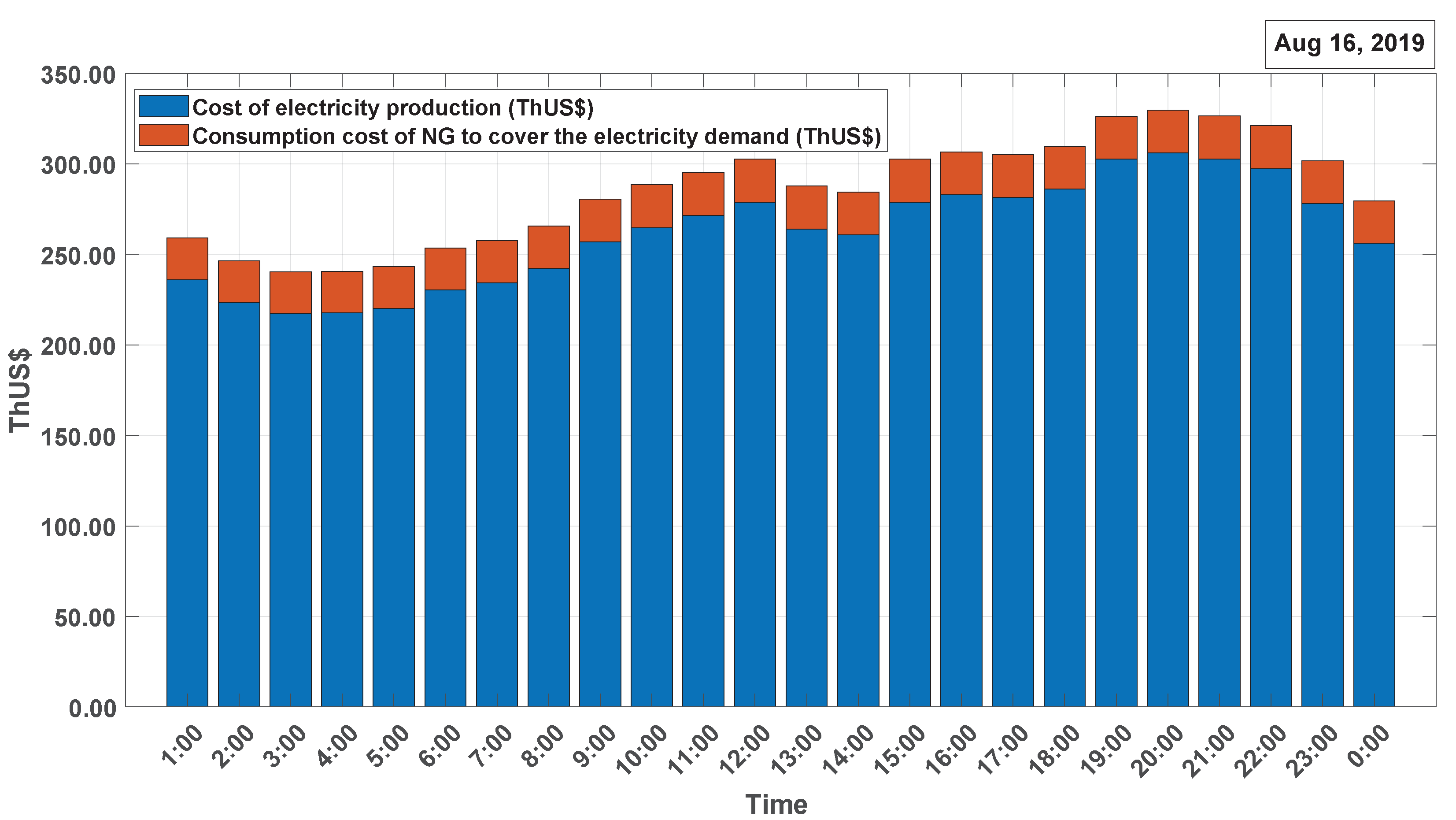
The results of the proposed method for the integrated natural gas and electricity system, for stage 1, are shown in Figure 8, where the cost associated with the production of electricity and the cost of supply and operation of NG to cover the electricity demand can be seen, also considering the dispatch of NG for the non-electric demand. It can be observed that the behavior of the production cost correlates with demand, not presenting greater distortion, only due to consideration of whether it is in peak hour or off-peak hour. It can be observed that the highest operating cost of the system for scenario 1 occurs at 8:00 p.m., with a cost of USD 329,750, which is an operating cost found during the peak hour of the system. The total daily production cost of the integrated system in stage 1 is USD 6.85 million.

Figure 9 shows the dispatch energy by type of technology derived from the optimization of production costs for the entire integrated gas–electricity system.

In this stage, the contribution of the natural gas-fueled thermoelectric power from bus 6 to bus 12 is constant throughout the day (780 MW), and the flow from bus 12 to bus 4 has a range between 716.00 and 349.33 MW, in a somewhat similar way, they happen with the flow from bus 6 to bus 5 being constant throughout the day (632 MW), and the flow from bus 10 to bus 5 oscillate between 378.43 and 269.20 MW, due to the transmission constraint and the specific locations of the hydroelectric plants, as well as the behavior of the demand in that area. This proposed method helps generators to achieve economic dispatch energy, the costs of optimizing the integrated gas electricity market with NG plants and pipelines in that area, the implementation of renewable power plants, and energy accumulators.

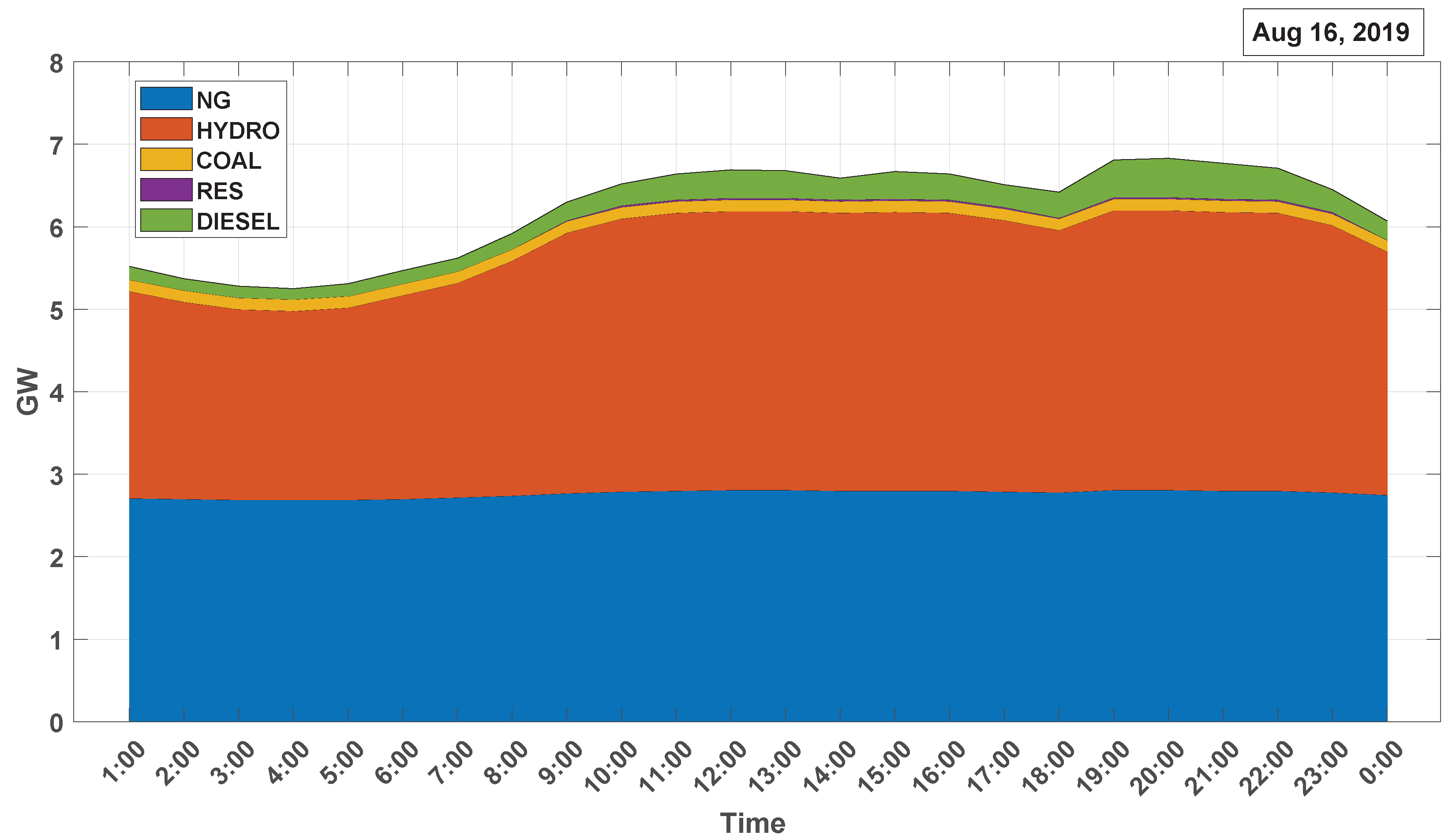
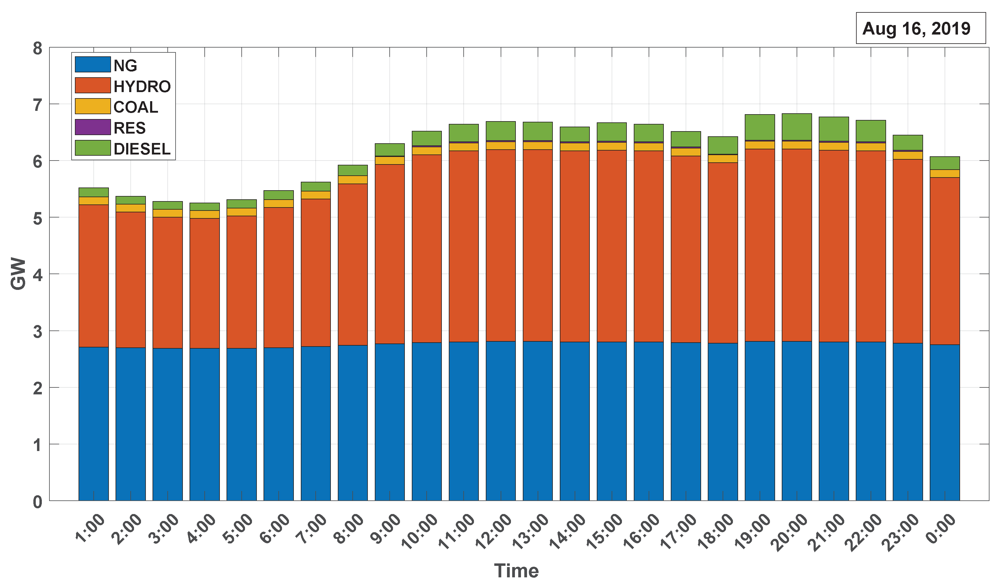
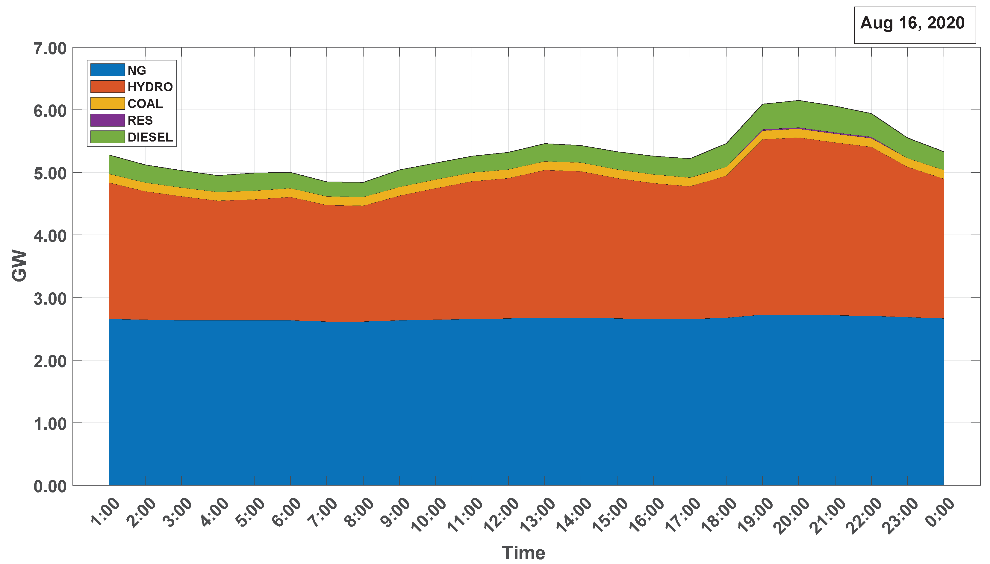
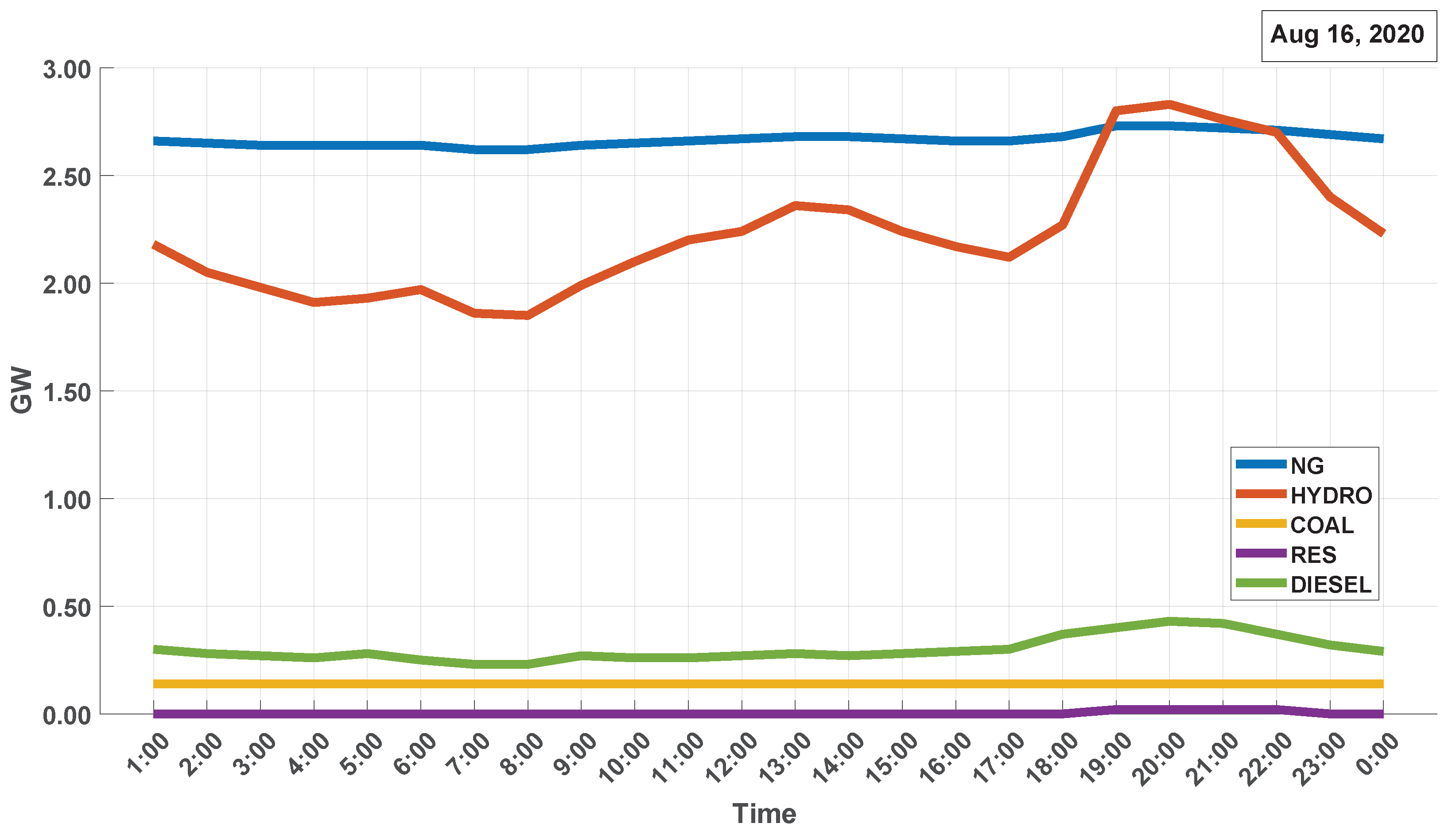
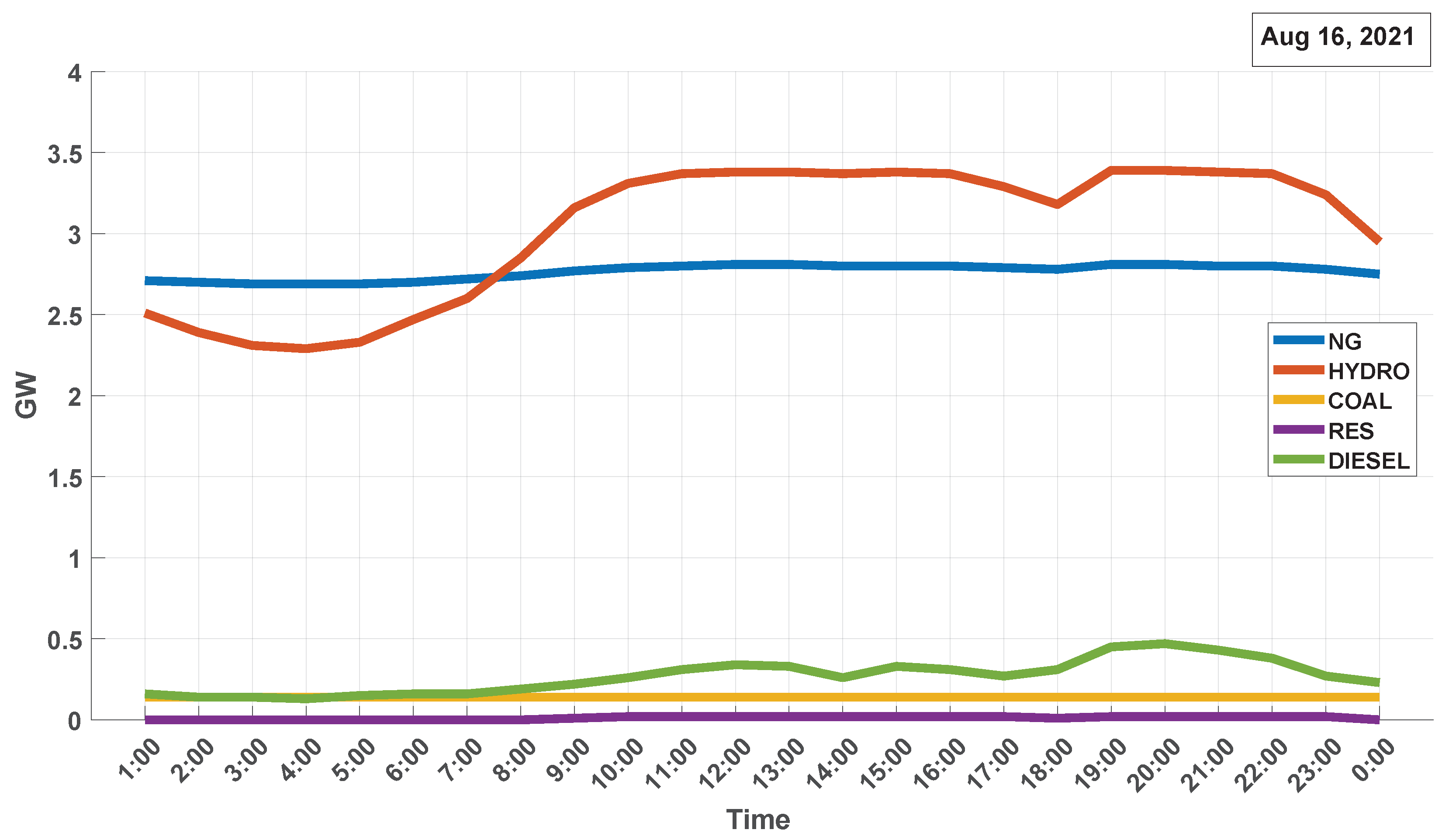
Figure 10 and Figure 11 show the contributions for each type of technology (hydraulic, NG, coal, residual, and diesel) for stage 1 in a comparative and aggregate way.

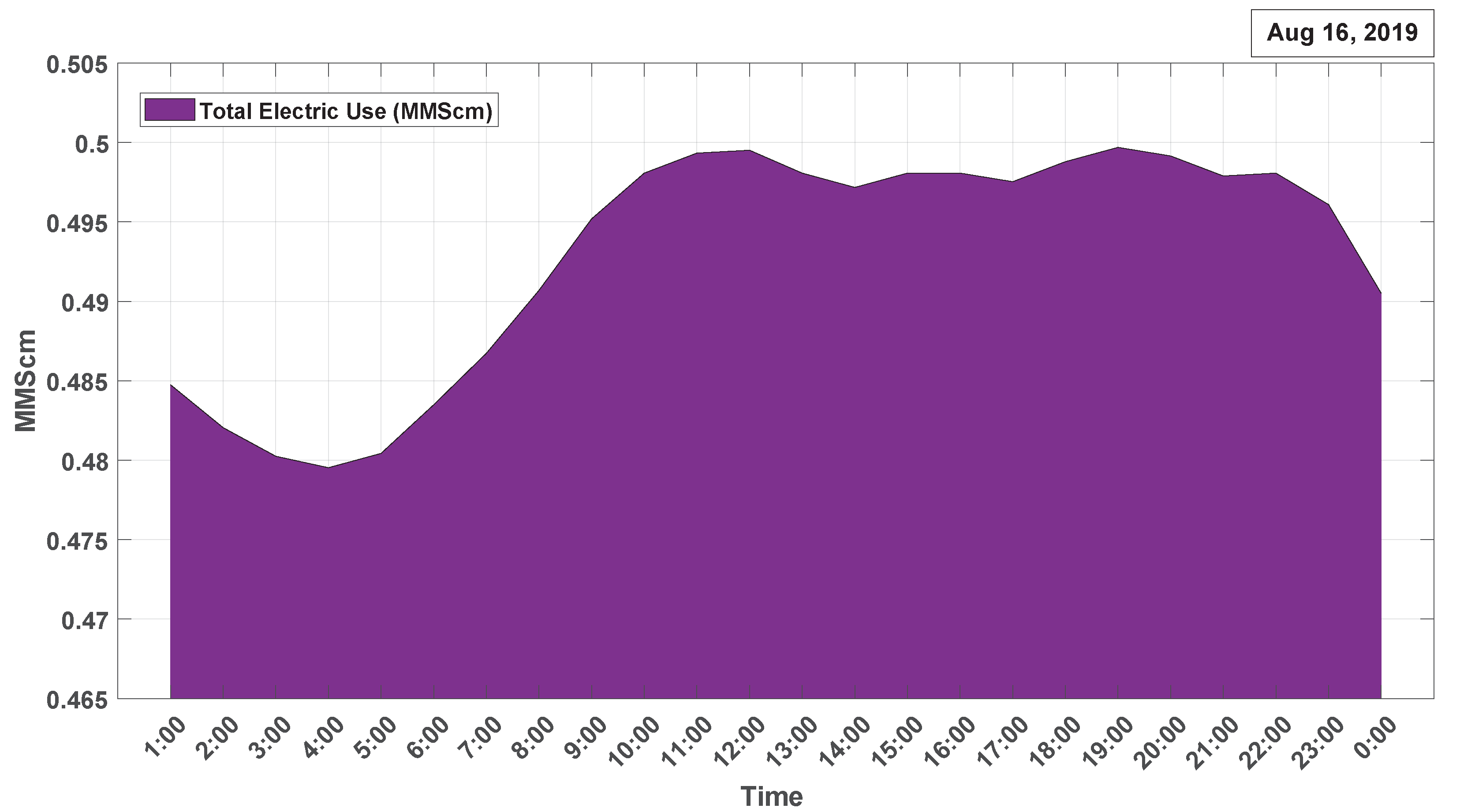
Concerning the dispatch of NG for strictly electrical use, the result of this optimization shows in Figure 12 the behavior of the NG demand for stage 1. the natural gas demand has a variation between 0.48 and 0.50 MMScm, which shows that, with this demand under normal conditions, the physical restrictions of the pipeline do not generate effects on the dispatch. Finally, the total consumption of NG to supply electricity demand is 11.82 MMScm for USD 563,880.

4.2. Stage 2—In a State of Health Emergency

During the health emergency, there was a drop in electricity consumption, which can be observed in Figure 13, showing the cost associated with the production of electricity and natural gas to cover the electricity demand in this stage.

The cost of production, in stage 2, also shows a correlation with demand, not presenting a major distortion only due to the consideration of whether it is peak hour or off-peak hour.

It can be seen that the highest operating cost for the system in stage 2 occurs at 20:00. (peak hour) with a cost of USD 286,230, which is an operating cost much lower than other scenarios. The reduction in demand for the electric system is mainly due to the lockdown management and social restrictions of the COVID-19 pandemic controls.

Figure 14 shows the dispatch energy by type of technology derived from the optimization of production costs for the entire integrated gas–electricity system, of stage 2, which supplies each of the buses of the equivalent model of the SEIN.

It is observed that the economic dispatch of the thermal generation plants in stage 2 is very similar to the load dispatch of the NG plants in stage 1, the dispatch logic does not vary, prioritizing the lower generation prices of thermal power above hydroelectric plants, even though this is a “pandemic stage”. However, unlike stage 1, a particular detail is presented because the contribution of NG generation to the north through the flows from bus 6 to bus 12 remained constant throughout the day (780 MW). However, for bus 12 to bus 4, their flows reduced between 593.00 and 367.33 MW. Similarly, the contribution of generation to NG to the south through the flows from bus 6 to bus 5 remained constant throughout the day (632 MW) despite the reduction in demand. However, the flows from bus 10 to bus 5 had their flows reduced between 329.34 and 221.50 MW. Unlike scenario 1, a particular detail is presented because the contribution of NG generation towards the south through the flows from bus 7 to bus 8 presented a strong variability, ranging from 184 MW in peak hours to 245 MW in off-peak hours, which is seen as strange but not an illogical situation, as this is due to the need to maintain the voltage profile in the bus with hydraulic power plants, and the strong reduction in demand due to the lockdown management and social restriction of the COVID-19 pandemic. On the other hand, the flows from bus 4 to bus 3 also showed marked variability, ranging from 223 MW in off-peak hours to 373 MW in peak hours; this behavior is derived from the transmission constraints and the location of the hydroelectric plants. as well as the behavior of demand in the southern region, minimally impacting the effects of the reduction in demand due to 451 COVID-19.

In the same way, Figure 15 and Figure 16 show the contributions for each type of technology (hydraulic, NG, coal, residual, and diesel) for stage 2 in a comparative and aggregated way.

Regarding the dispatch of natural gas for strictly electrical use, in Figure 17, the result of this optimization shows that the behavior of the NG demand for stage 2 in a state of sanitary emergency has variation in a range between 0.472 and 0.492 Millions-Scm, showing us that with this demand, under normal conditions the physical restrictions of the pipeline do not generate effects on the dispatch. Likewise, the total consumption of NG to supply electricity demand is 11.53 Millions-Scm at a total cost of USD 549,390.

It can also be indicated that by comparing the consumption of NG for electrical use, the demand for NG was somewhat affected by the effect of the state of emergency by COVID-19.

4.3. Stage 3—Lifted the State of Health Emergency

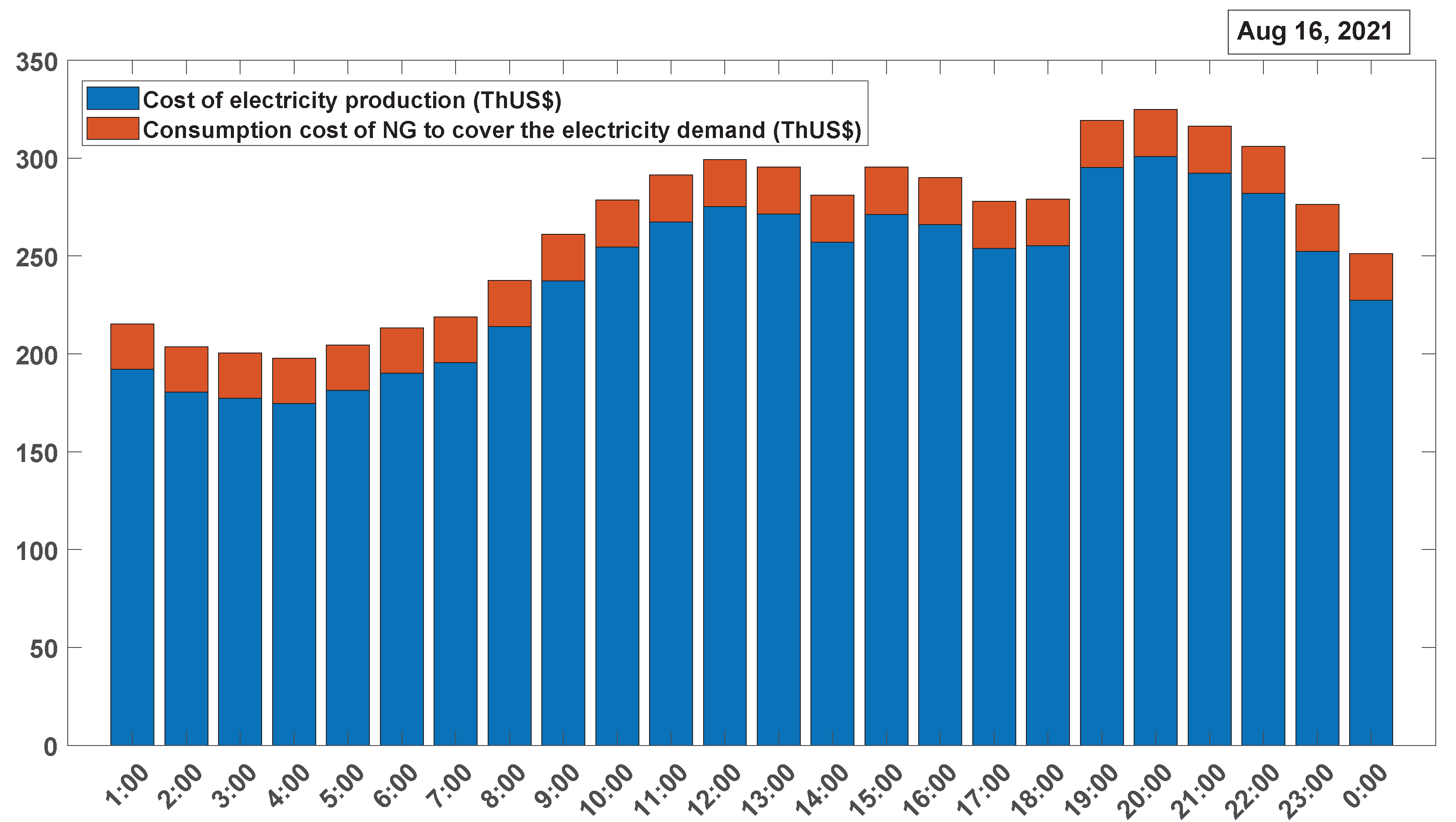
After the restrictions imposed by COVID-19, there was an increase in gas consumption. Figure 18 shows the cost associated with producing electricity and NG to cover the electricity demand, also considering the NG dispatch for non-electrical demand in stage 3.

It can be seen that the highest operating cost of the system for stage 3 occurs at 8:00 p.m. with a cost of USD 324,930, which is an operating cost that is well below production costs before the state of emergency due to COVID-19. The total daily cost of production of the integrated system in stage 3 is USD 6.34 million, a cost of production still far below the production costs before the pandemic.

Figure 19 shows the energy dispatch by type of technology derived from cost optimization for the entire integrated gas–electricity system, which supplies each of the buses of the equivalent SEIN model for stage 3, lifted the state of health emergency as a result of COVID-19.

The dispatch of the load from the thermal generation plants in Stage 3 is observed. As in stage 1, the priority in dispatch has the hydroelectric generation plants, as well as thermal generation with NG due to the lower prices. However, it can be observed in this stage that, despite the lower demand of the system, the contribution of the generation to NG toward the south through the flow from bus 5 to bus 9 is constant throughout the day, as in stage 1 (635 MW), in a somewhat similar way, it happens with the flows from bus 5 to bus 11, oscillating between 109.39 and 120.41 MW, with a small reduction compared to stage 1, and whose behavior is derived by the restrictions of the transmission and the location of the hydroelectric plants and to the behavior of the demand in the southern region.

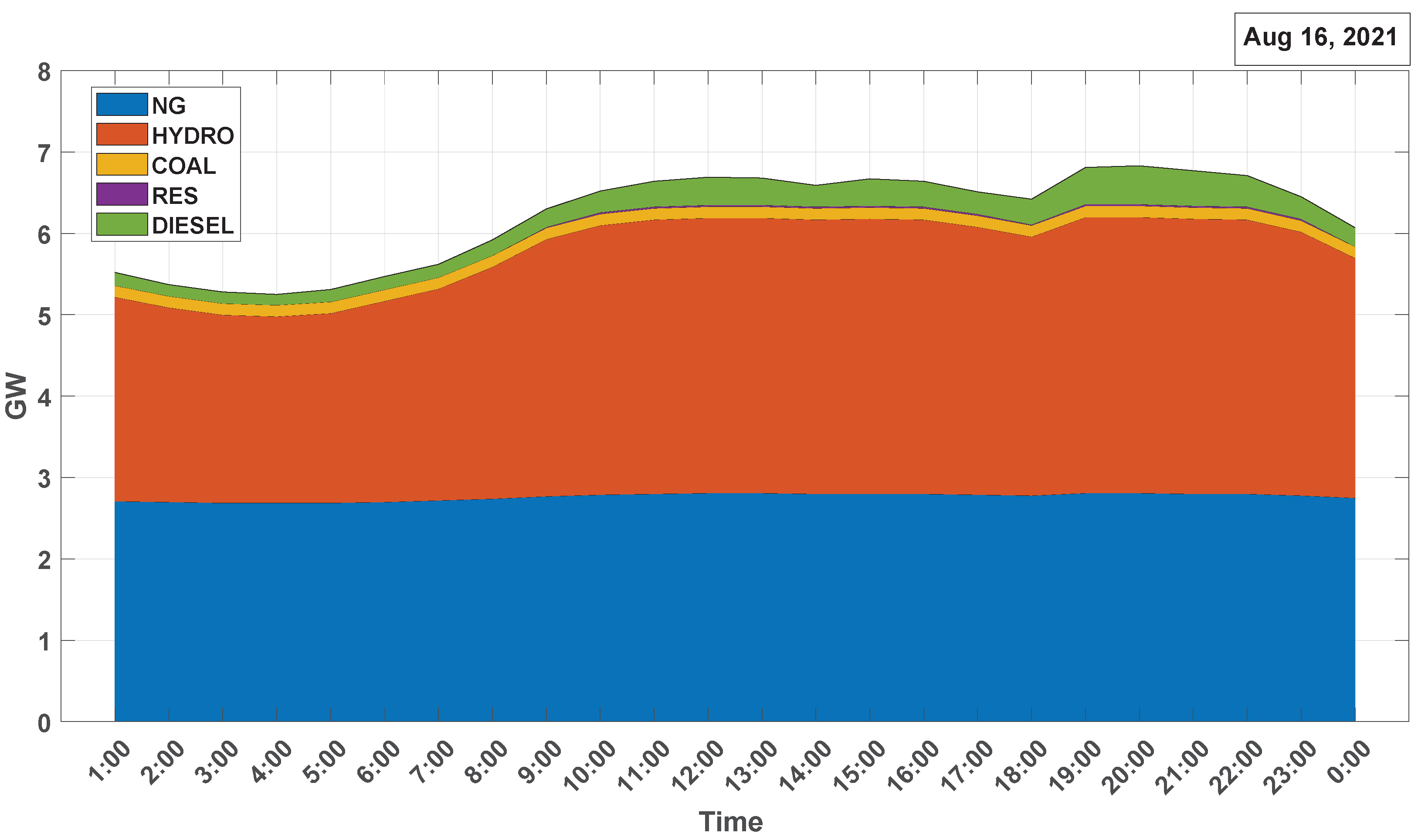
From the result of the optimization in Figure 20 and Figure 21, the contributions for each type of technology (hydraulic, NG, coal, residual, and diesel) are shown for stage 3 in a comparative and aggregated way.

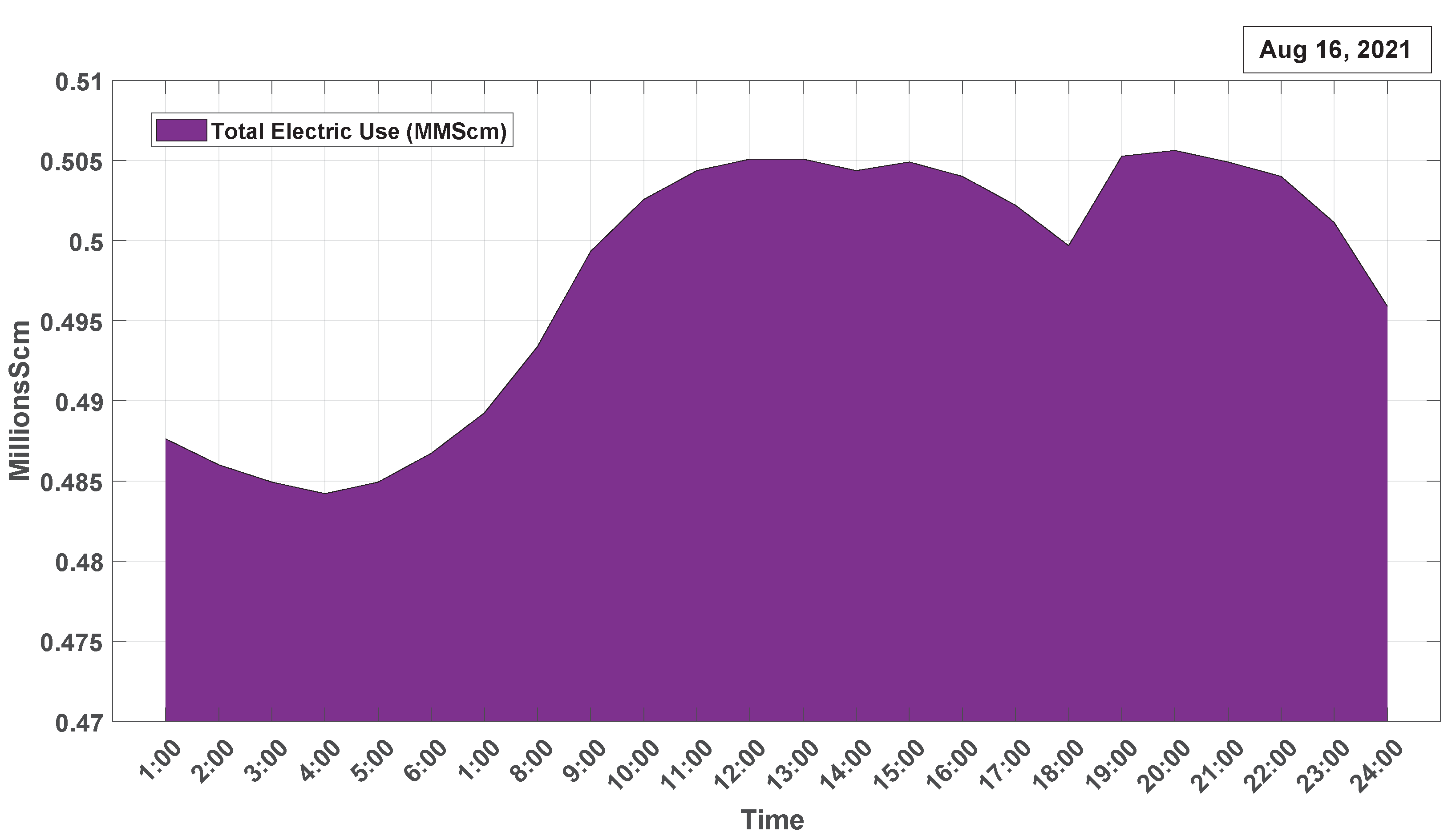
Figure 22 shows the behavior of the NG demand for stage 3, lifting the state of sanitary emergency; the NG demand varying between 0.484 and 0.506 Millions-Scm, it shows us that, with this demand, under normal conditions, the physical restrictions of the pipeline do not generate effects on the dispatch. Likewise, the total consumption of NG to supply electricity demand is 11.94 Millions-Scm at a total cost of USD 569,440 Although these results also show a slight recovery in gas demand and its production costs, they do not reach those obtained before the pandemic.

Scenarios Comparison

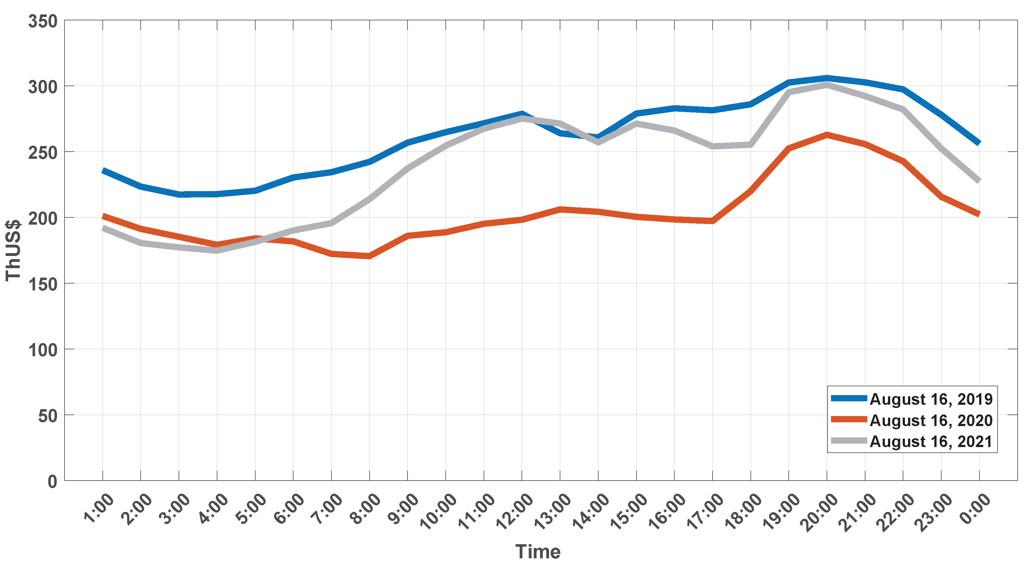
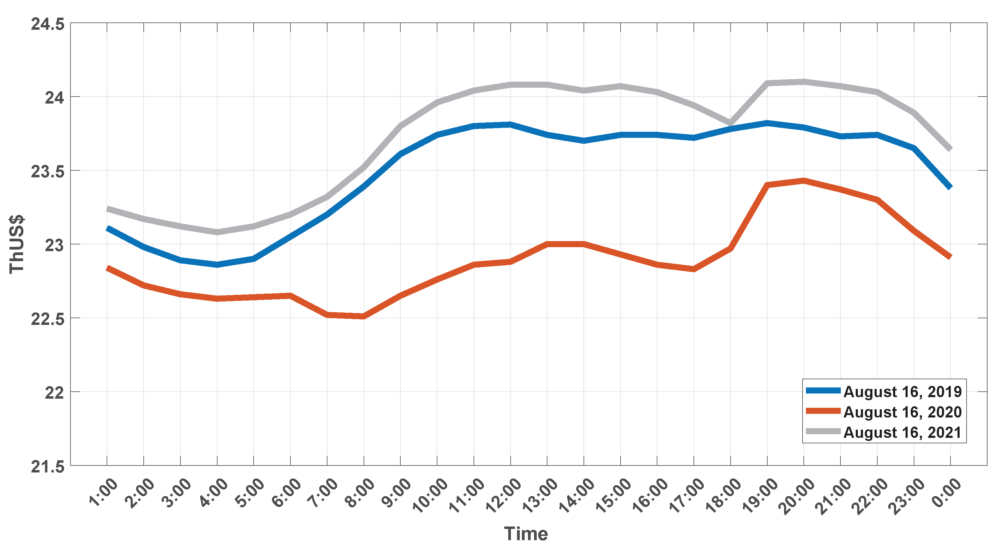
Figure 23 shows the optimal cost behavior of the integrated gas–electricity system for the three stages. It can be seen that, in the stages (e.g., stages of low demand due to restrictions derived from the state of health emergency), the behavior of the costs follows the behavior of demand.

However, in stage 1, between 4:00 and 9:00 p.m., the behavior changes, due to the entry of other generators with lower marginal costs that previously did not enter, due to restrictions of the network itself, which can be observed in detail in Figure 24, reflecting the optimal costs of production of electricity for each stage.

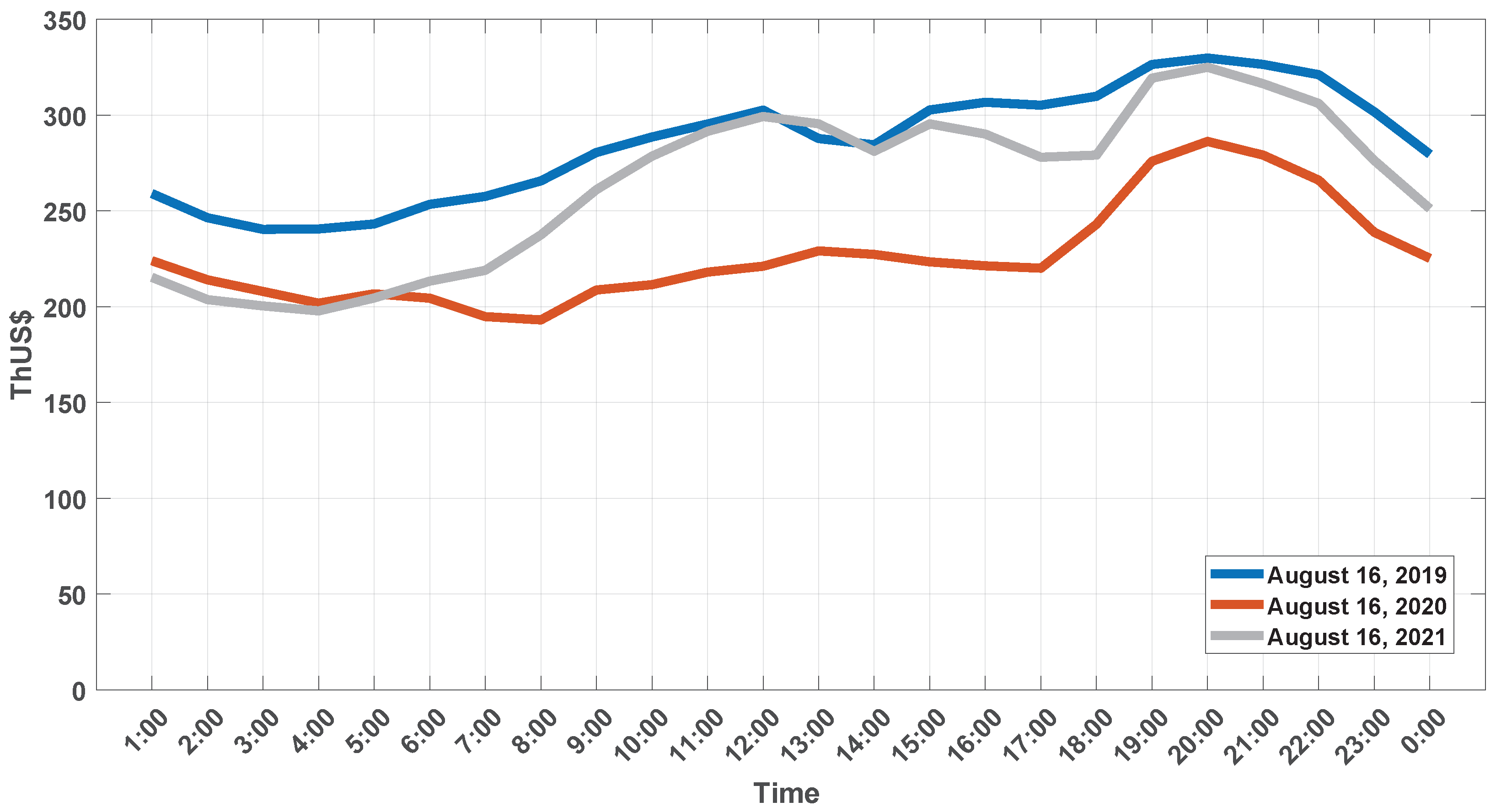
Regarding the optimal cost of NG consumption to cover the electrical demand Figure 25, it is observed that there are indeed differences in the marginal costs of NG consumption although the demand for NG—very similar in stages 1 and 3—but if a significant difference is observed in stage 2. This is due to the lower demand for NG in the Chilca plants, derived not from the inability to deliver energy, but from the network’s restrictions, which require other plants to dispatch energy in order to maintain network parameters, such as transmission limits and voltage profile.

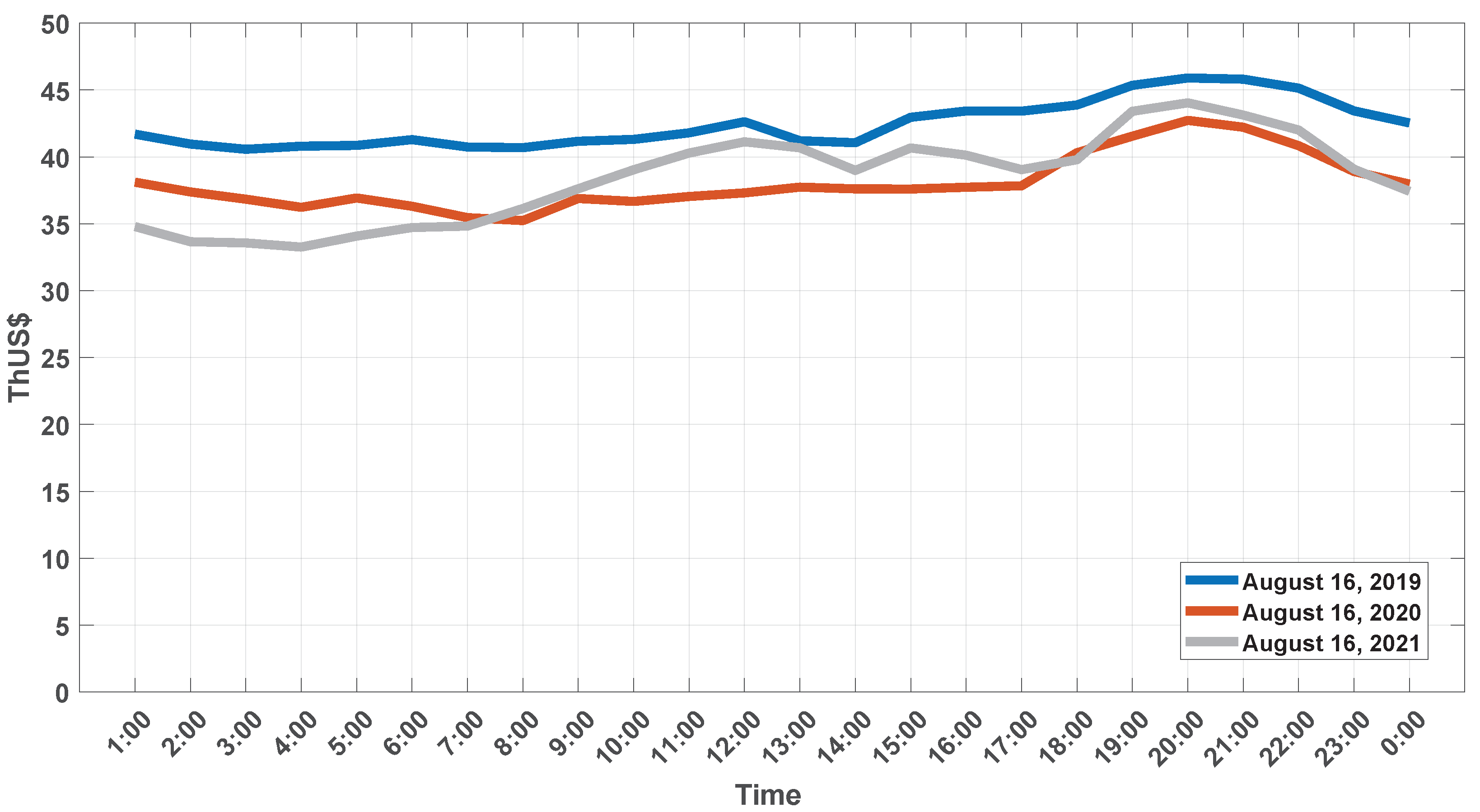
Figure 26 shows us the variation of the optimal average cost for each stage, in which the behavior of the average cost of stage 1 can be observed, between the hours of 4:00 and 9:00 p.m., for the entry of other generators with lower marginal costs that previously did not enter due to restrictions of the network itself.

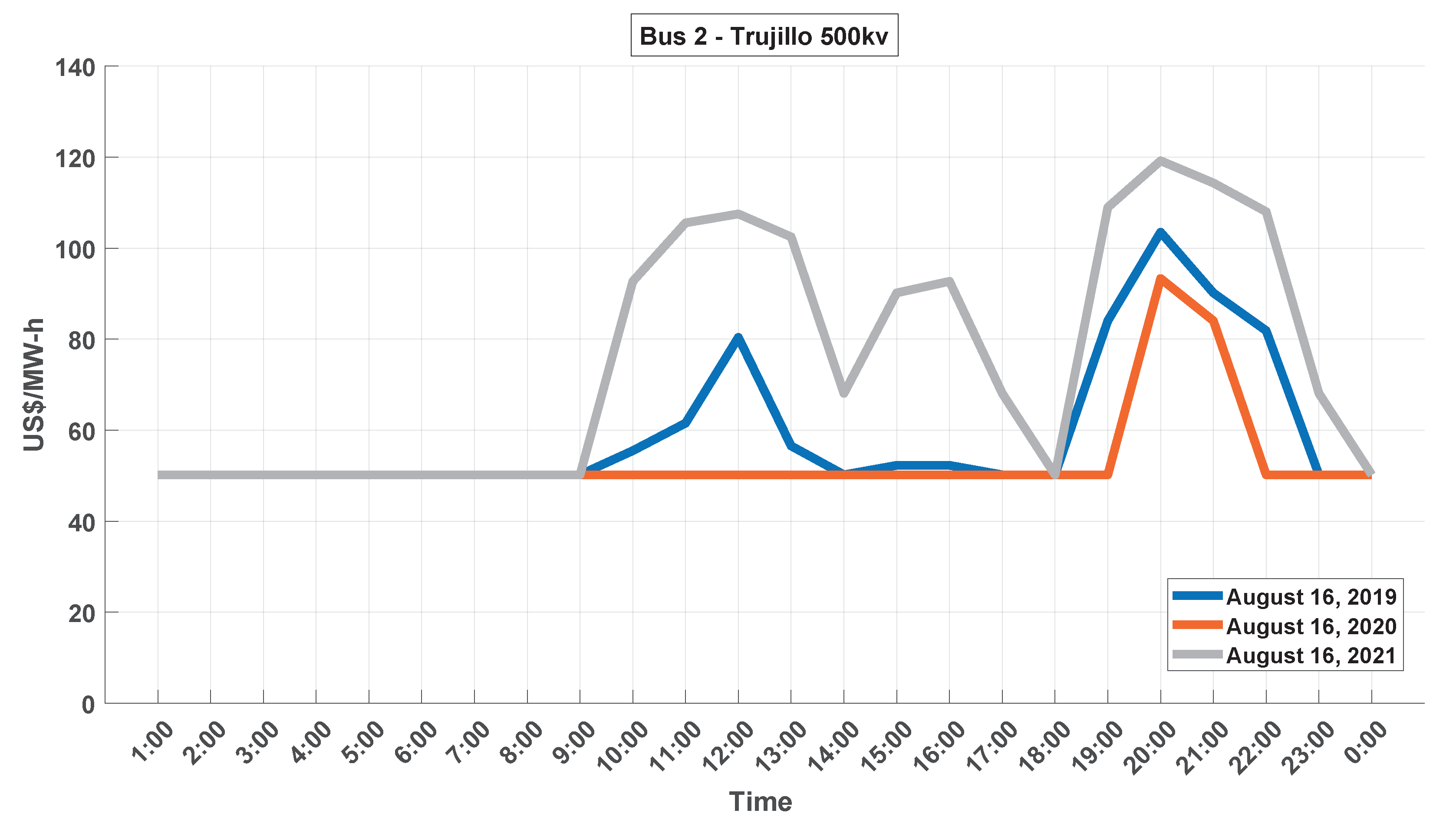
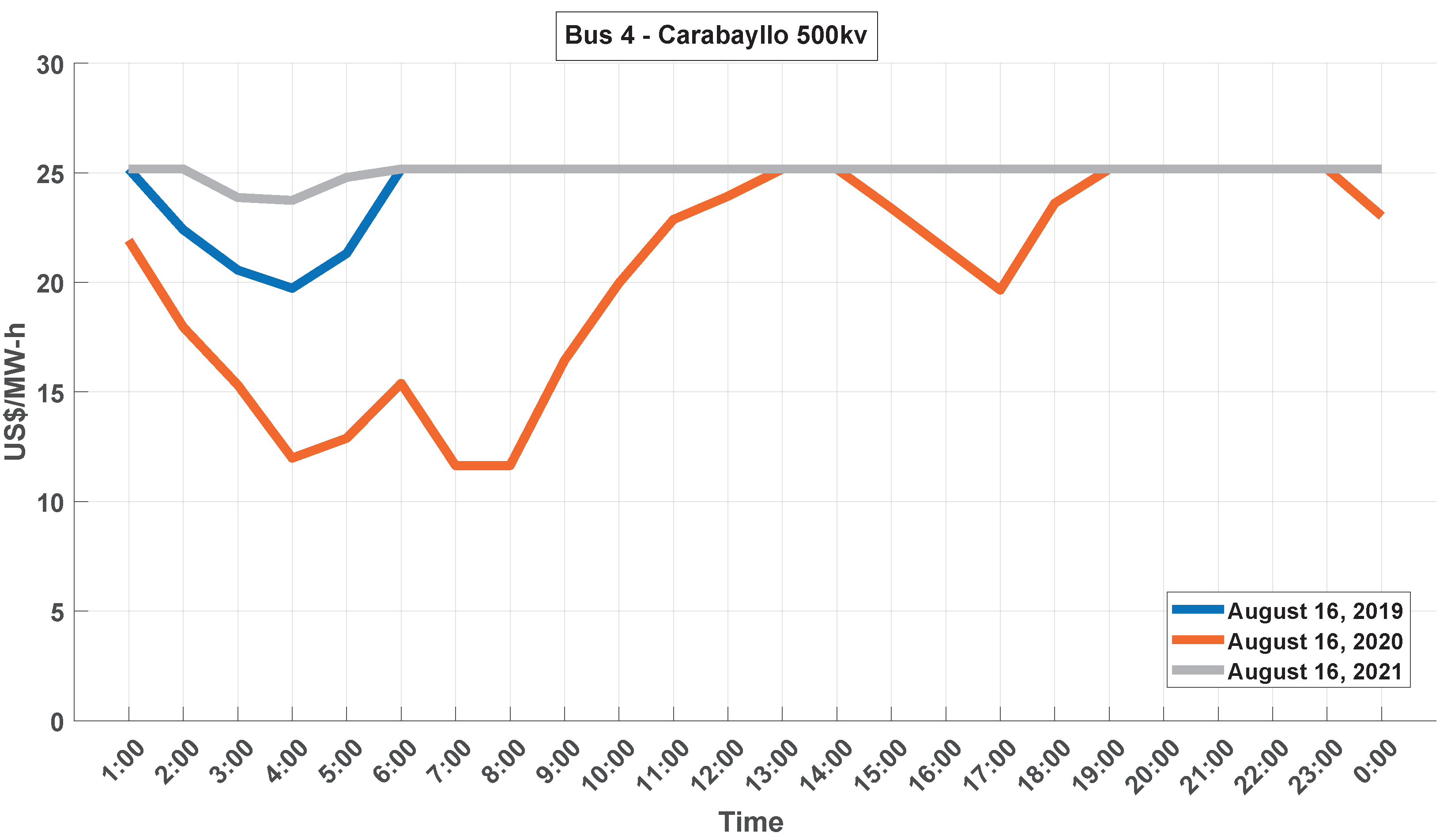
Figure 27 and Figure 28 show the variations of the bus prices; it is possible to observe the variations of the bus prices per hour in each stage. It is to be expected that, given the lower energy demand, the bus price tends to fall with the presence of natural gas-fueled thermoelectric and hydroelectric units without the presence of operation of diesel or residual thermoelectric plants.

Figure 28 shows the power flow from bus 5 (the bus where the NG thermal generation plants are concentrated) to bus 9. For stages 1 and 3, it is the same (491 MW), even when, in stage 3, the demand of the system is lower due to pandemic restrictions being lifted. However, for stage 2, there is a marked variability that ranges between 418.14 and 328.77 MW. This behavior results from the transmission constraints, as well as the location of hydroelectric plants and the demand in the southern region due to the restrictions imposed by COVID-19.

In all stages, there are invariable load flows throughout the day, such as the flow between bus 5 and bus 6 (632MW), between bus 5 and bus 9 (491 MW), and between bus 6 and bus 12 (780 MW); this is because the transmission constraints limit the power flow transmission to cover the demands.

Figure 29 shows a comparative way the flows from bus 6 (where the NG thermal generation plants are concentrated) to bus 5, showing that the flows vary as the demand ‘demands’ them; however, as the pandemic restrictions were lifted in stage 3, it can be observed that, as the demand increased, the transmission line began to saturate up to around 632.80 MW; this behavior is derived from the transmission constraints.

Figure 30 shows the behavior of the load flows between bus 4 and bus 3 for the different scenarios, where variability is observed due to congestion problems in the network, as a result of the transmission constraints that did not exceed 378 MW.

Figure 31 shows the behavior of the power flows from bus 12 to bus 4 for different stages, observing a marked variability of the power flows in this transmission line, ranging from 302 MW in the off-peak hours up to 807 MW in the peak hours. This maximum level of capacity of the transmission line corresponds to the limits of the transmission line.

Finally, Figure 32 shows the behavior of the power flows from bus 8 to bus 9, in this transmission line, which even came, at times, to changes in the directionality of power flows, as observed in stage 3, where flows changed direction from −18 MW in off-peak hours to 47 MW in peak hours; this change in the directionality was because, in this period, social conflicts were submitted, which reduced the demand in the south of the country.

5. Computer Performance

The integrated electricity and gas system is a complex problem involving thousands of buses connected to hundreds of gas nodes, as well as the restrictions of both networks, making a complex matrix of equations out of their processing. For the case of the integrated electricity system with 12 bus and natural gas networks with 7 nodes in Peru, the model solution presents 7515 equations, 8595 variables, and 8280 restrictions, turning into a complex computational problem.

The CPU processing time to resolve the problem was 3 min 22 s and 239 milliseconds. The simulations were performed using the GAMS WEX VS8 2.5.1 Model Statistic Solve Overall on a computer with an Intel Core i7 2.40 GHz processor and 12 GB RAM.

6. Conclusions

Our main research contribution is the systematic presentation of qualitative and quantitative analyses of the interdependence of natural gas and electricity networks as an integrated gas–electricity system. Simulating with real energy dispatch values in three stages: stage 1, before the entry into force of supreme decree no. 044-2020-PCM dated 15 March 2020, “Supreme Decree that declares a State of National Emergency for the serious circumstances that affect the life of the Nation as a result of the COVID-19 outbreak”; stage 2, in the midst of a state of health emergency; and stage 3, the state of health emergency was lifted.

This research led to the need to model the SEIN and gas pipeline networks as an integrated model, this gas–electricity system describes the physical characteristics of the networks, to calculate the maximum social benefit or minimum social costs of supplying electric energy at the lowest costs of production, with minimum costs of natural gas supplies, and whose results allowed us to address the implementation of policies for the integration of electricity and gas markets, mitigating the effects of congestion in the NG transportation pipeline and restrictions on electrical transmission.

The determination of the optimal dispatch for an integrated gas–electricity system, considering the effects of constraint transmission in the competition of the gas and electricity market, shows the need for the coordination of both markets, to obtain greater efficiencies and lower operating costs in energy dispatch.

Therefore, improving the coordination between both systems through a single market operator cannot only obtain better optimal operating costs as a whole of the electricity and NG grid systems, as has been shown in the research, but can also help improve the reliability of NG supply to power producers.

Comparing costs in each stage, some outstanding aspects can be observed: stages 2 and 3 are stages of low demand due to the restrictions derived from the state of a health emergency, the behavior of the production cost and energy supply, and natural gas operation of the integrated gas–electricity system and the optimal cost of electricity production follow the behavior of demand.

A significant difference is observed in stage 2, due to the lower demand for natural gas that serves to cover the electricity demand in the power stations located at bus 6, derived not from the inability to deliver energy, but due to the grid’s constraints, which require other plants to dispatch energy to maintain voltage profile.

Regarding the variation of bus prices, little price stability is observed at bus 2 and bus 4, in stage 2, due to the lower demand for energy and the oversupply of generation capacity, since the model prioritizes the dispatch of plants with cheaper costs, such as NG and hydraulic generation, recovering, as the demand for energy also recovers.

The model shows us how the restrictions on transmission have generated—that the behavior of the supply of generation using natural gas, for energy transfers to the southern zone, is restricted, even when the prices of generation using natural gas are below hydroelectric generation prices, such as in stage 2 and stage 3, presenting transmission lines with saturated power flows caused by bus prices, resulting in higher operating costs.

Finally, several pending issues will allow for future research into renewable sources and operational flexibility assets, such as energy storage facilities, etc., showing that there is a need to incorporate additional equations into the model.

References

- Jenkins, S.E. Interdependency of Electricity and Natural Gas Markets in the United States: A Dynamic Computational Model. Master’s Thesis, MIT, Cambridge, MA, USA, 2014. [Google Scholar]
- Jenkins, S.; Annaswamy, A.; Hansen, J.; Knudsen, J. A dynamic model of the combined electricity and natural gas markets. In Proceedings of the 2015 IEEE Power Energy Society Innovative Smart Grid Technologies Conference (ISGT), Washington, DC, USA, 18–20 February 2015; pp. 1–5. [Google Scholar] [CrossRef]
- Erdener, B.C.; Pambour, K.A.; Lavin, R.B.; Dengiz, B. An integrated simulation model for analysing electricity and gas systems. Int. J. Electr. Power Energy Syst. 2014, 61, 410–420. [Google Scholar] [CrossRef]
- Gil, M.; Dueñas, P.; Reneses, J. Electricity and Natural Gas Interdependency: Comparison of Two Methodologies for Coupling Large Market Models Within the European Regulatory Framework. IEEE Trans. Power Syst. 2016, 31, 361–369. [Google Scholar] [CrossRef]
- Ward, J.B. Equivalent circuits for power-flow studies. Electr. Eng. 1949, 68, 794. [Google Scholar] [CrossRef]
- Subdirección de Programación del COES, P.d.M.D. Database in DIgSilent Format Available in Annex 2, Electrical Analysis of the Daily Intervention Program Report. 2020. Available online: https://www.coes.org.pe/Portal/operacion/progoperacion/programadiario (accessed on 28 March 2021).
- Tostado-Véliz, M.; Arévalo, P.; Jurado, F. A comprehensive electrical-gas-hydrogen Microgrid model for energy management applications. Energy Convers. Manag. 2021, 228, 113726. [Google Scholar] [CrossRef]
- Ventosa, M.; Baillo, A.; Ramos, A.; Rivier, M. Electricity market modeling trends. Energy Policy 2005, 33, 897–913. [Google Scholar] [CrossRef]
- Martínez, P.D. Analysis of the Operation and Contract Management in Downstream Natural Gas Markets. Ph.D. Thesis, University Pontificia Comillas, Madrid, Spain, 2013. [Google Scholar]
- de Energía y Minas, M. Resolución Ministerial Nro 102-2020-MINEM/DM del 27 de marzo de 2020, Proyecto de Decreto Supremo que aprueba el Reglamento para Optimizar el Uso del Gas Natural y Creación del Gestor del Gas Natural. 2020. Available online: https://cdn.www.gob.pe/uploads/document/file/572362/RM_102_2020_MINEM_DM.pdf.pdf (accessed on 28 March 2021).
- Rubio, R.; Ojeda-Esteybar, D.; Ano, O.; Vargas, A. Integrated natural gas and electricity market: A survey of the state of the art in operation planning and market issues. In Proceedings of the 2008 IEEE/PES Transmission and Distribution Conference and Exposition: Latin America, Bogota, Colombia, 13–15 August 2008; pp. 1–8. [Google Scholar] [CrossRef]
- Munoz, J.; Jimenez-Redondo, N.; Perez-Ruiz, J.; Barquin, J. Natural gas network modeling for power systems reliability studies. In Proceedings of the 2003 IEEE Bologna Power Tech Conference Proceedings, Bologna, Italy, 23–26 June 2003; Volume 4, p. 8. [Google Scholar] [CrossRef]
- Mello, O.D.; Ohishi, T.T. An integrated dispatch model of gas supply and thermoelectric generation with constraints on the gas supply. In Proceedings of the 2005 5th Power Systems Computation Conference, Liège, Belgium, 22–26 August 2005; Session 18, Paper 5, pp. 1–6. Available online: https://services.montefiore.uliege.be/stochastic/pscc05/papers/fp528.pdf (accessed on 28 March 2021).
- Urbina, M.; Li, Z. A Combined Model for Analyzing the Interdependency of Electrical and Gas Systems. In Proceedings of the 2007 39th North American Power Symposium, Las Cruces, NM, USA, 30 September–2 October 2007; pp. 468–472. [Google Scholar] [CrossRef]
- Unsihuay, C.; Lima, J.W.M.; de Souza, A.Z. Modeling the Integrated Natural Gas and Electricity Optimal Power Flow. In Proceedings of the 2007 IEEE Power Engineering Society General Meeting, Tampa, FL, USA, 24–28 June 2007; pp. 1–7. [Google Scholar] [CrossRef]
- An, S.; Li, Q.; Gedra, T. Natural gas and electricity optimal power flow. In Proceedings of the 2003 IEEE PES Transmission and Distribution Conference and Exposition (IEEE Cat. No.03CH37495), Dallas, TX, USA, 7–12 September 2003; Volume 1, pp. 138–143. [Google Scholar] [CrossRef]
- Liu, C.; Shahidehpour, M.; Fu, Y.; Li, Z. Security-Constrained Unit Commitment With Natural Gas Transmission Constraints. IEEE Trans. Power Syst. 2009, 24, 1523–1536. [Google Scholar] [CrossRef]
- Li, T.; Eremia, M.; Shahidehpour, M. Interdependency of Natural Gas Network and Power System Security. IEEE Trans. Power Syst. 2008, 23, 1817–1824. [Google Scholar] [CrossRef]
- Hecq, S.; Bouffioulx, Y.; Doulliez, P.; Saintes, P. The integrated planning of the natural gas and electricity systems under market conditions. In Proceedings of the 2001 IEEE Porto Power Tech Proceedings (Cat. No.01EX502), Porto, Portugal, 10–13 September 2001; Volume 1, p. 5. [Google Scholar] [CrossRef]
- Unsihuay-Vila, C.; Marangon-Lima, J.W.; de Souza, A.C.Z.; Perez-Arriaga, I.J.; Balestrassi, P.P. A Model to Long-Term, Multiarea, Multistage, and Integrated Expansion Planning of Electricity and Natural Gas Systems. IEEE Trans. Power Syst. 2010, 25, 1154–1168. [Google Scholar] [CrossRef]
- Bezerra, B.; Barroso, L.A.N.; Kelman, R.; Flach, B.D.C.; de Lujan Latorre, M.; Campodonico, N.M.; Pereira, M.V.F. Integrated Electricity–Gas Operations Planning in Long-term Hydroscheduling Based on Stochastic Models. In Handbook of Power Systems I; Springer: Berlin/Heidelberg, Germany, 2010; pp. 149–175. [Google Scholar]
- Chaves, F.S. Otimização da operação da rede de gás natural para suprimento das termelétricas por programação não-linear. Bachelor’s Thesis, Engenharia Eletrica, Escola Politécnica, Universidade Federal do Rio de Janeiro, Rio de Janeiro, Brazil, 2010. [Google Scholar]
- de planificación del COES, S. Estudios de Verificación del Margen de Reserva Firme Objetivo del Sistema para el Periodo 2020–2023. 2020. Available online: https://www.coes.org.pe/Portal/Planificacion/MargenReserva/ (accessed on 28 March 2021).
- Group, W. Common Format For Exchange of Solved Load Flow Data. IEEE Trans. Power Appar. Syst. 1973, PAS-92, 1916–1925. [Google Scholar] [CrossRef]
- Wolf, D.D.; Smeers, Y. The Gas Transmission Problem Solved by an Extension of the Simplex Algorithm. Manag. Sci. 2000, 46, 1454–1465. [Google Scholar] [CrossRef] [Green Version]
- Wolf, D.D. Mathematical Properties of Formulations of the GN transmission problem. Teh. Glas. 2017, 3, 133–137. [Google Scholar]
- Osinergmin. Demanda del 04/06/2019. Available online: https://www.osinergmin.gob.pe/Resoluciones/Resoluciones-GRT-2021.aspx (accessed on 28 March 2021).
Figure 1.
Single line electrical diagram in 500, 220, and 138 kV (88 bus). (SEIN-COES).
Figure 2.
Non-linear reduced equivalent model of SEIN at 500 kV for the year 2020 (12-bus).
Figure 3.
NG Transportation network (extracted from Osinergmin).
Figure 4.
Diagram of the transportation capacity of the Peruvian gas pipeline (adapted from Osinergmin).
Figure 5.
Equivalent model of the Peruvian NG network (adapted from Osinergmin [27]).
Figure 6.
Diagram of the Peruvian gas–electricity interaction.
Figure 7.
Electrical demands by stage.
Figure 8.
Optimal cost of energy production and ng supply and operation of the integrated gas–electricity system—stage 1.
Figure 9.
Contribution to the dispatch of the electrical system—stage 1.
Figure 10.
Contribution to the dispatch by type of technology—stage 1.
Figure 11.
Contribution added to the dispatch by type of technology—stage 1.
Figure 12.
Demand for NG for electric use—stage 1.
Figure 13.
Optimal cost of energy production and ng supply and operation of the integrated gas–electricity system—stage 2.
Figure 14.
Contribution to the dispatch of the electrical system—stage 2.
Figure 15.
Contribution to demand by type of technology—stage 2.
Figure 16.
Contribution added to the dispatch by type of technology—stage 2.
Figure 17.
Demand for NG for electric use—stage 2.
Figure 18.
Optimal cost of energy production and ng supply and operation of the integrated gas–electricity system—stage 3.
Figure 19.
Contribution to the dispatch of the electrical system—stage 3.
Figure 20.
Contribution to demand by type of technology—stage 3.
Figure 21.
Contribution added to the dispatch by type of technology—stage 3.
Figure 22.
Demand for NG for electric use—stage 3.
Figure 23.
Optimal cost of energy production and ng supply and operation of the integrated gas–electricity system by stage.
Figure 24.
Optimal cost of electricity production by stage.
Figure 25.
Optimal cost of ng consumption to cover electricity demand by stage.
Figure 26.
Variation of the optimal average cost of electricity by stage.
Figure 27.
Variations of the spot price by stage (bus 2).
Figure 28.
Variations of the bus prices by stage (bus 4).
Figure 29.
Power flow variation from bus 6 to bus 5 (MW).
Figure 30.
Power flow variation from bus 4 to bus 3 (MW).
Figure 31.
Power flow variation from bus 12 to bus 4 (MW).
Figure 32.
Power flow variation from bus 8 to bus 9 (MW).