Analysis of the Influence of Parameter Condition on Whole Load Power Factor and Efficiency of Line Start Permanent Magnet Assisted Synchronous Reluctance Motor

Abstract

Line start permanent magnet assisted synchronous reluctance motor (LSPMaSynRM) is an important high-efficiency and high-quality motor. Its parameter matching and operating characteristics are complex, with an increase in salient ratio resulting in a valley in the power factor curve. In this study, the formation principle of power factor curve valley was first deduced by the mathematical model of LSPMaSynRM. Then, the parameter matching principle of power factor curve valley was analyzed in detail. On this basis, the characteristics of load rate corresponding to the critical state of the power factor curve valley were obtained, and its influence on whole load efficiency was analyzed. The design principles for optimal efficiency in wide high-efficiency region and specific load point were obtained. Finally, a 5.5 kW LSPMaSynRM was designed and manufactured to verify the validity of the principle.

1. Introduction

High-efficiency, light-weight, and high-quality motor systems are the basic component of high-end equipment in the field of engineering. Permanent magnet synchronous motor (PMSM) has the advantages of high efficiency and high power density [1,2]. It is often used in high-quality motor but requires high cost. Without permanent magnet material, synchronous reluctance motor (SynRMs) relies on reluctance torque to drive the motor. Its cost is low, but its power factor and torque density are also low. Meanwhile, its current is large, and it is difficult for it to be efficient and light.

Permanent magnet assisted synchronous reluctance motor (PMaSynRM) is a special permanent magnet motor that combines the respective characteristics of PMSM and SRM [3]. Reasonable selection and design of rotor blades can improve the salient ratio and power factor of PMaSynRM to reduce the running current. At the same time, the performance of the motor can be optimized under certain constraints by optimizing the matching of permanent magnet torque [4,5].

Many studies have been carried out in this field, including the aspects of power factor and efficiency. In [6], the influence of the shapes of flux barriers and the number of “rotor virtual slots” was investigated based on the multiphysics model, which can achieve low vibration for PMSynRMs. In [7], in order to obtain maximum torque and minimum torque ripple in the design, optimal values of motor parameters were obtained by improving the rotor geometry of the three-phase PMaSynRM. In [8], the influence of permanent magnet flux linkage on power factor was analyzed, and it was proposed that the power factor could be raised to more than 0.8 when the permanent magnet flux linkage was more than 3 times the q-axis. In [9], a PMaSynRM prototype with four poles was designed by placing ferrite magnets inside the rotor of a SynRM, and experimental measurements were performed under various loading conditions. In [10], the optimizing rotor structure was found to improve the power factor, with the power factor of the prototype increasing from 0.879 to 0.918. In [11], the power factor was found to increase from 0.35 to 0.63 by adding AlNiCo on the basis of synchronous reluctance motor. In [12,13], the multilayer magnetic barrier structure was considered, and it was shown that the choice of the first permanent magnet thickness had a great influence on the power factor. In [14], the shape parameters were used to redefine the load rate so as to realize optimization of the load rate to meet the requirements of high efficiency. In [15], a simple structure was proposed with the topology composed of an internally inserted V-shape permanent magnet (IVPM) machine and a synchronous reluctance machine (SynRM). The main novelty was that the PMs in the rotor were diverted so that the reluctance component of the torque and the magnetic component of the torque reached their maximum values at the same load angle, which eventually led to a higher output torque for the same volume. In [16], a PM-assisted- SynRM design was proposed for high torque performance. Although it used the torque components to the fullest, it suffered from high torque ripple and relatively complex rotor geometry. In [17], time-stepping FEM and multiobjective genetic algorithm were used to optimize PMaSynRM, which improved the motor efficiency to more than 92% under rated working conditions and met the IE4 standards. In [18], a two-pole multibarrier ferrite-assisted SynRM for water pumps was designed, with the prototype having high power factor and efficiency. Many scholars have analyzed the operating characteristics of PMaSynRM, such as efficiency and power factor, but most of them have focused on specific rotor structure and geometric parameters. There have been few studies on the efficiency and power factor characteristics of PMaSynRM in the whole load range from the perspective of parameter matching.

In this study, the formation principle of power factor curve valley was deduced by the mathematical model of LSPMaSynRM. The deduction was not confined to any specific rotor structure so that the conclusion could be universal. On this basis, the matching of parameters and the characteristics of the corresponding load rate were analyzed in detail. Then, further analysis of the impact on whole load efficiency was carried out. Finally, a 5.5 kW LSPMaSynRM was designed and manufactured to verify the validity of the principle.

2. Analysis of the Principle of Power Factor Curve Valley of PMaSynRM

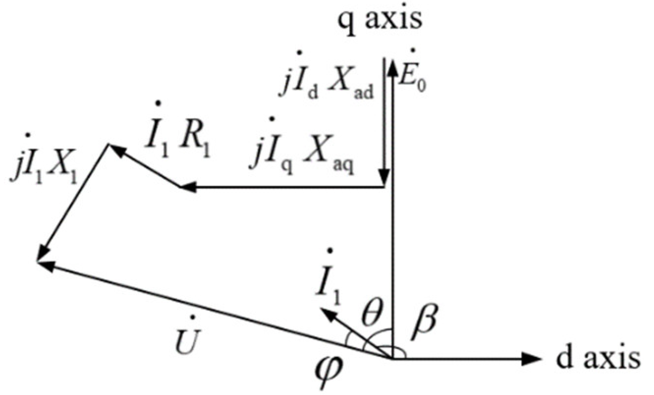
Power factor is the rate of active power to apparent power, which is essentially the phase relationship between the voltage and current in a specific operating state of the motor determined by parameters under the determination of torque. According to the mathematical model of PMaSynRM, the torque equation can be obtained as follows:

$$T_e=\frac{mp{E}_{0}U}{\omega X_{\mathrm{d}}}\sin \theta +\frac{mp{U}^2}{2\omega }(\frac{1}{X_{\mathrm{q}}}-\frac{1}{X_{\mathrm{d}}})\sin 2\theta$$

(1)

where T_e is electromagnetic torque, m is the number of phases, p is poles, E₀ is no-load back electromotive force (EMF), θ is the angle between voltage and no-load back EMF, U is voltage, ω is angular frequency, X_d is d-axis reactance, and X_q is q-axis reactance. The vector diagram was shown in Figure 1.

The torque equation can also be expressed as follows:

$$T_e=p[{\psi }_{\mathrm{f}}{i}_{\mathrm{s}}\sin \beta +\frac{1}{2}(L_{\mathrm{d}}-L_{\mathrm{q}})i_s^2\sin 2\beta ]$$

(2)

where ψ_f is permanent magnet flux linkage, β is the angle between current and permanent magnet flux linkage, i_s stator current, L_d is d-axis inductance, and L_q is q-axis inductance.

In sine steady state, the torque equation can be changed as follows:

$$T_e=mp[\frac{E_0}{\omega }{I}_{\mathrm{s}}\sin \beta +\frac{1}{2}(L_{\mathrm{d}}-L_{\mathrm{q}})I_{\mathrm{s}}^2\sin 2\beta ]$$

(3)

Ignoring resistance, the d-axis and q-axis current are as follows:

$$I_{\mathrm{d}}=\frac{E_0-U\cos \theta }{X_{\mathrm{d}}}$$

(4)

$$I_{\mathrm{q}}=\frac{U\sin \theta }{X_{\mathrm{q}}}$$

(5)

The stator current can be expressed as follows:

$$I_{\mathrm{s}}=\sqrt{{(\frac{E_0-U\cos \theta }{X_{\mathrm{d}}})}^2+{(\frac{U\sin \theta }{X_{\mathrm{q}}})}^2}$$

(6)

Putting it into torque Equation (3), the torque equation can be expressed as follows:

$$\begin{array}{l}{T}_e=\frac{mp{E}_0}{\omega }\sqrt{{(\frac{E_0-U\cos \theta }{X_{\mathrm{d}}})}^2+{(\frac{U\sin \theta }{X_{\mathrm{q}}})}^2}\sin \beta \\ +\frac{mp}{2\omega }(X_{\mathrm{d}}-X_{\mathrm{q}})[{(\frac{E_0-U\cos \theta }{X_{\mathrm{d}}})}^2+{(\frac{U\sin \theta }{X_{\mathrm{q}}})}^2]\sin 2\beta \end{array}$$

(7)

Torque is a function of θ and β. Equation (1) shows that the shape of the torque curve depends on E₀, U, X_d, and X_q, and the torque increases as θ increases. Equation (7) shows that the shape of the torque curve depends on E₀, U, X_d, X_q, and θ. For a manufactured motor, E₀, X_d, and X_q are constants, and U can also be regarded as a fixed value. As the torque increases, there is a one-to-one correspondence between θ and β. This corresponding relationship depends on the motor parameters E₀, U, X_d, and X_q, which can be attributed to two parameters, namely λ = E₀/U, which indirectly reflects the amount of permanent magnets, and the salient ratio ρ = X_q/X_d. Different parameters have different corresponding relationships between θ and β, which ultimately reflect different power factor curve states.

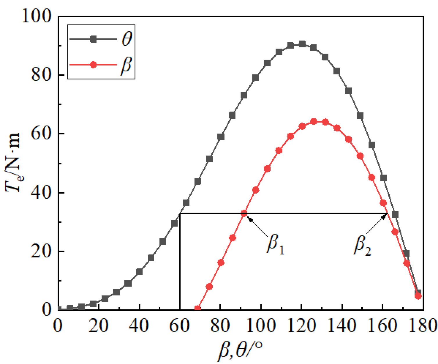
The relationship between θ and β can be obtained by simultaneous Equations (1) and (7). Because the equation is very complicated, it is impossible to obtain the analytical expression of the relationship. One solution of θ corresponding to two β can be obtained by numerical methods. According to the running state of the motor, the true solution and false solution can be judged as shown in Figure 2.

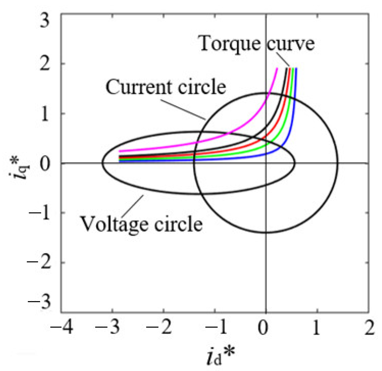
The introduction of the square term of θ in the process of deriving Equation (7) results in two β solutions. According to the voltage and torque equations, the voltage circle and the torque curve are obtained in the current plane of the d–q axis, and the true solution is obtained according to the intersection point, as shown in Figure 3.

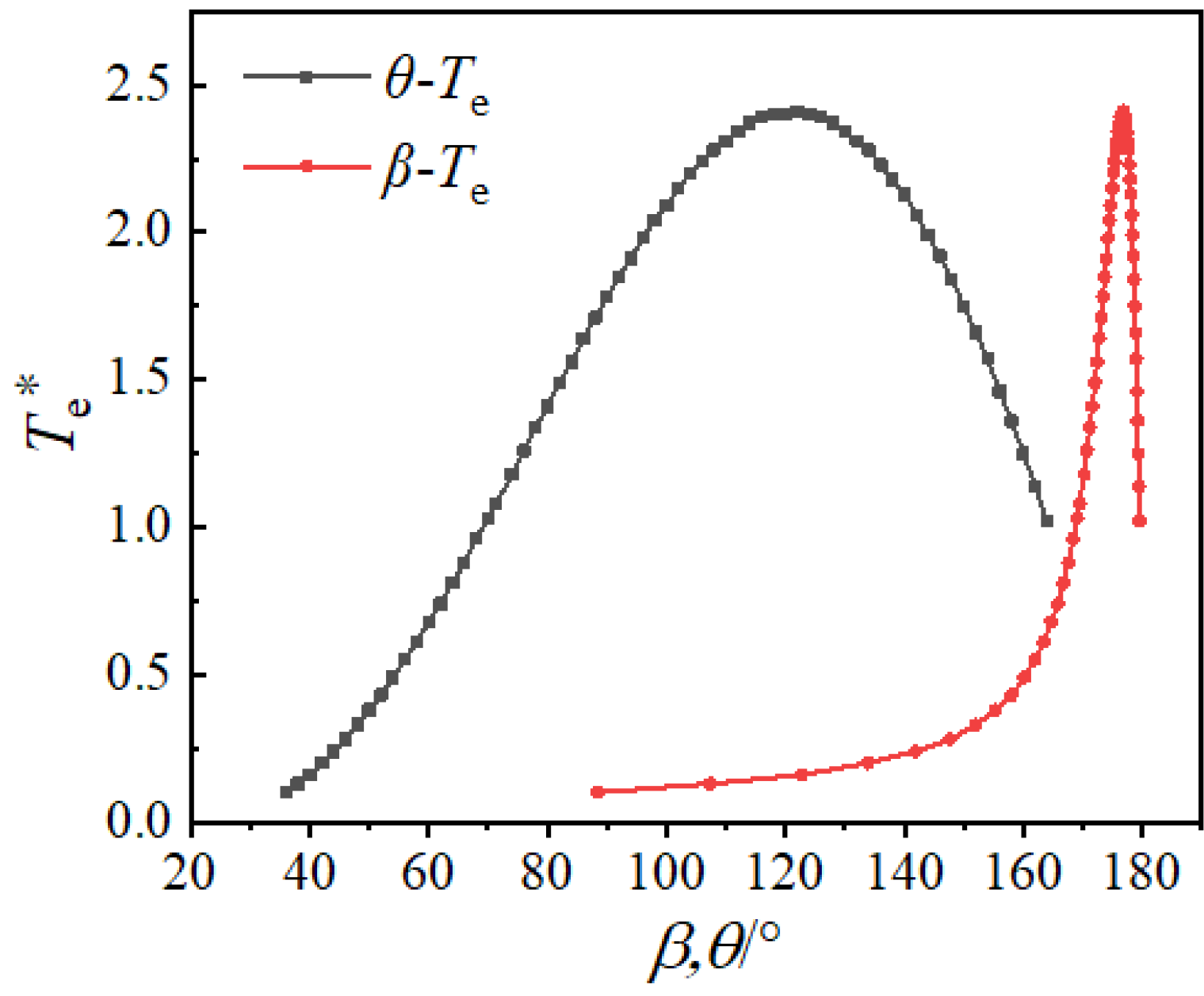
In this way, a torque curve with θ and β as independent variables can be obtained. The state of the curve depends on parameters λ and ρ. Under certain conditions, the two curves will have special states, as shown in Figure 4.

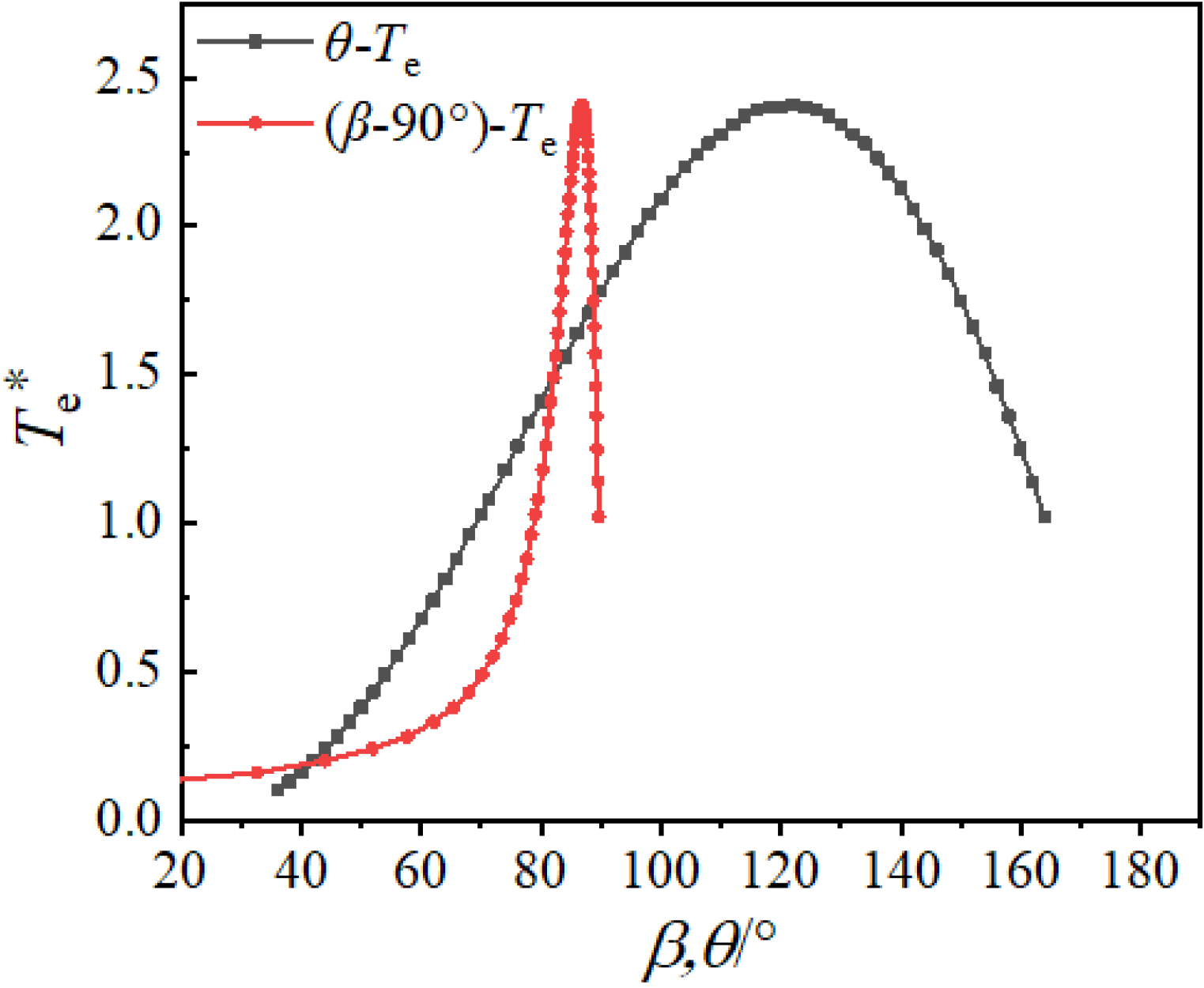
In order to observe the relationship of the curves more clearly, the β-T_e curve was shifted to the left by 90°, as shown in Figure 5. It can be seen that there are three intersections between the two curves, and the torque at the rightmost intersection is in the unstable range, so it will not be discussed. At the two intersections on the left, the two torque curves correspond to the same angle, and the power factor is 1. Between the crossing points and on both sides, the two curves of the same torque correspond to different angles, and the power factor is less than 1. This shows that there will be a valley in the power factor curve in the middle of two maximum values.

At the same time, the θ and β relationship curve and the power factor curve can be drawn as the torque increases. As shown in Figure 6, the valley in the power factor curve is apparent.

From the above analysis, it can be seen that the power factor curve valley is caused by two torque curves with two intersection points in the stable operating interval under matching parameters. It can also be understood that θ and β increase at different speeds.

3. The Influence of Parameter Matching on Power Factor Curve Valley of PMaSynRM and Its Corresponding Load Rate

3.1. The Condition of Power Factor Curve Valley and the Principle of Parameter Matching

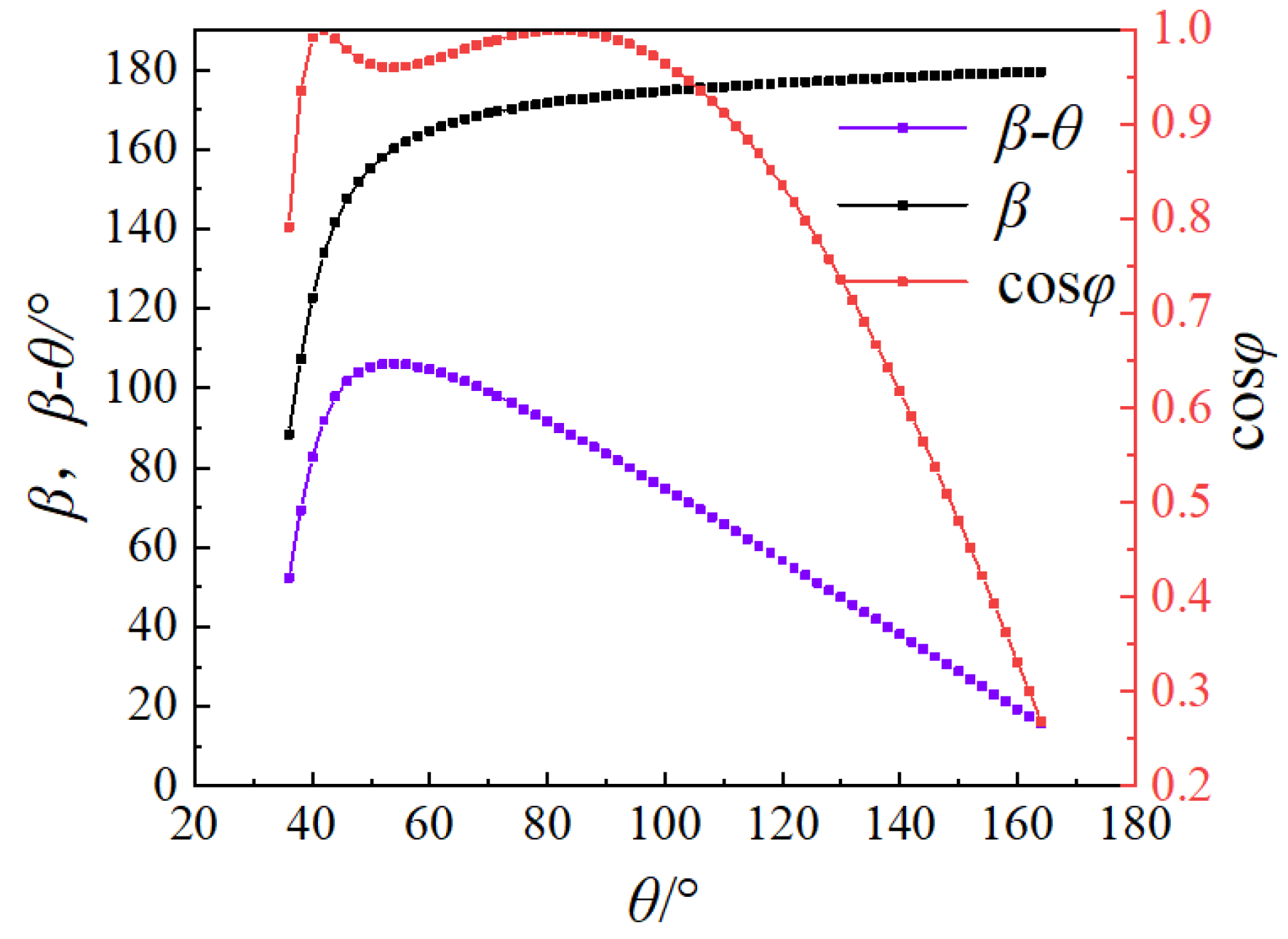
The analysis in the previous section shows that the power factor curve valley is caused by the increasing speed of θ and β being different as load increases. Therefore, the condition is that there is a β − θ > 90° state during load increases. Whether there is a state of β − θ > 90° depends on the parameters of the motor. Starting with the matching of λ and ρ, the principle that produces power factor curve valley are analyzed in this section.

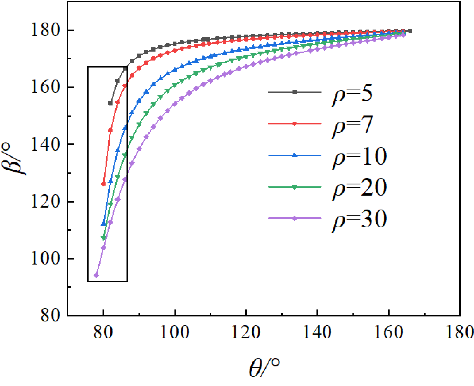
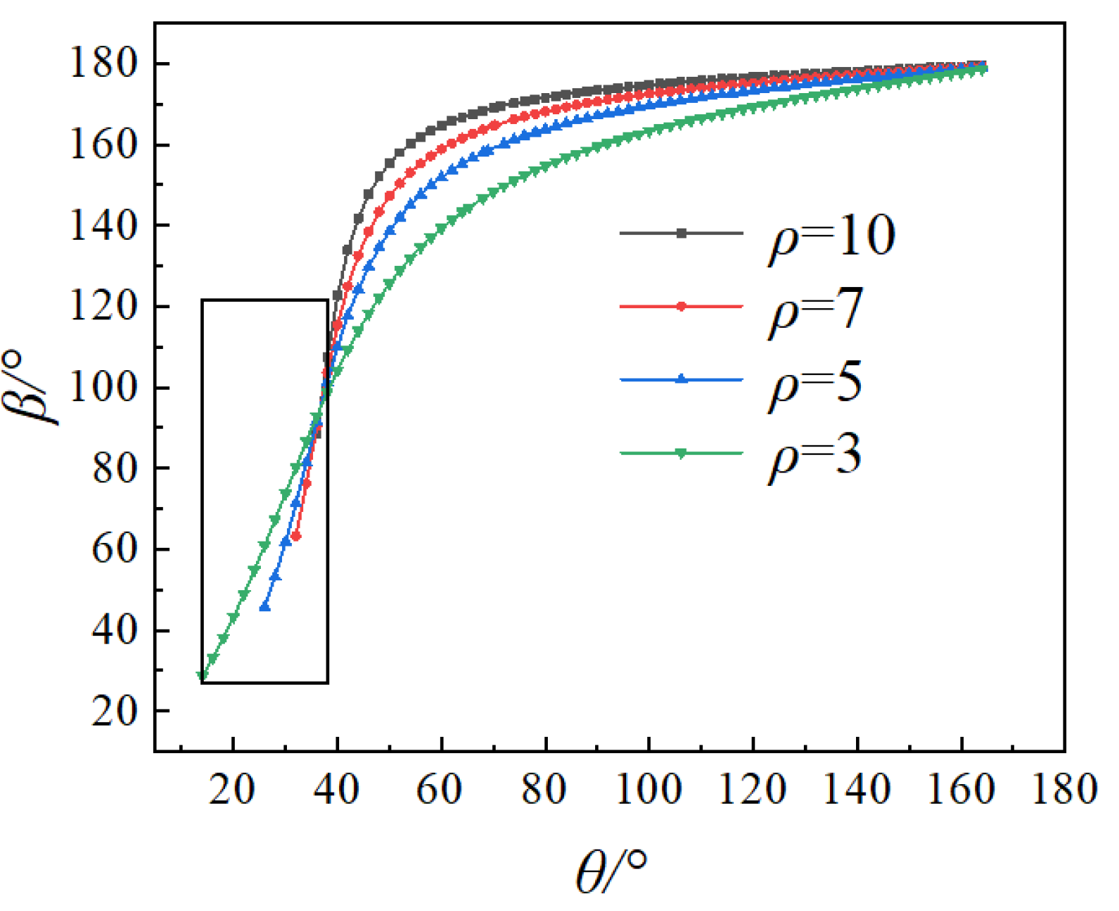
The change curves of β with θ under different salient ratio with λ = 0.2 are shown in Figure 6. With the increase in salient ratio, the middle part of curve stretches and protrudes to the upper left corner. The slope of the front part increases, but the slope of the back part decreases. This shows that as the salient ratio increases and as the load increases, the growth rate of β of the low load zone increases significantly, while the growth rate of β of the high load zone decreases. Throughout the whole load range, the value of β − θ increases first and then decreases. There must be a salient ratio state that makes a certain load point of β − θ = 90°, which can be called the critical point of the power factor curve valley. Then, there will be a valley on the power factor curve with increasing salient ratio. As can be seen from the rectangular box in Figure 7, the value of θ at the starting point of the curve is around 80°. As the salient ratio increases, the range of change is relatively small, but the range of change of β is relatively large.

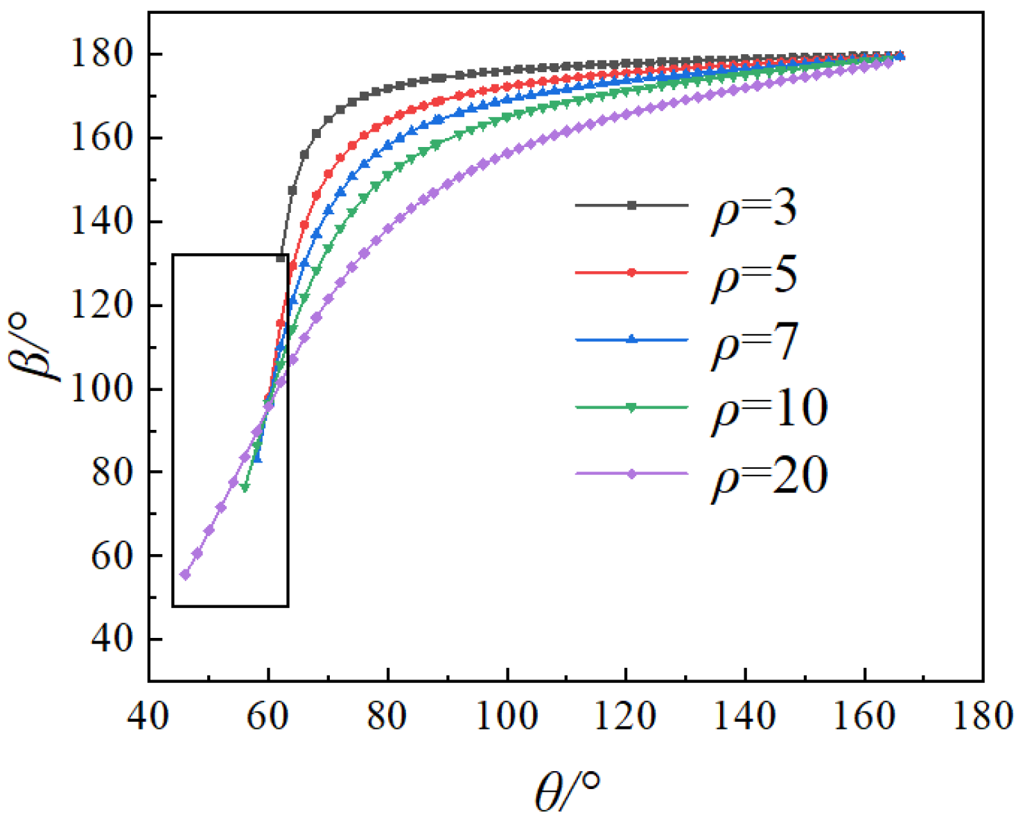
The change curves of β with θ are shown in Figure 8 for the condition of λ = 0.5. The state of the curves as the salient ratio increases is similar to Figure 7. The difference is that the initial value of θ in the rectangular box is about 60°.

The change curves of β with θ are shown in Figure 9 for the condition of λ = 0.8. The overall state of the curve is similar to Figure 7 and Figure 8, and the initial value of θ is further reduced to about 30°.

As can be seen from Figure 7, Figure 8 and Figure 9 as λ increases, the initial value of θ gradually decreases. The smaller the value of θ, the less difficult it is to reach β − θ > 90°, which means that it is easier for a valley to be formed on the power factor curve. At the same time, the distribution range of entire curve β and θ increases as λ increases.

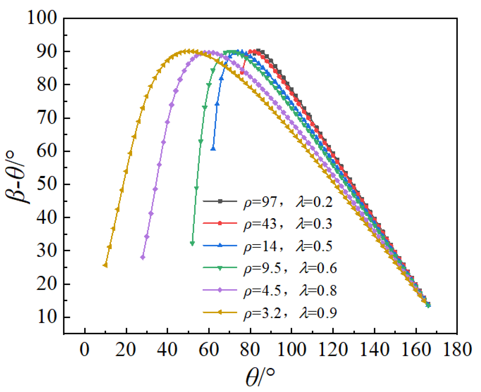
The above analysis shows that there are different parameter matching principles that result in a valley in the power factor curve. The states of β − θ = 90° can be obtained by calculation, as shown in Figure 10. The required salient ratio increases as λ decreases. As the corresponding critical point of the power factor curve valley value of θ increases, the distance to the initial point is closer and the initial value of β and θ are larger.

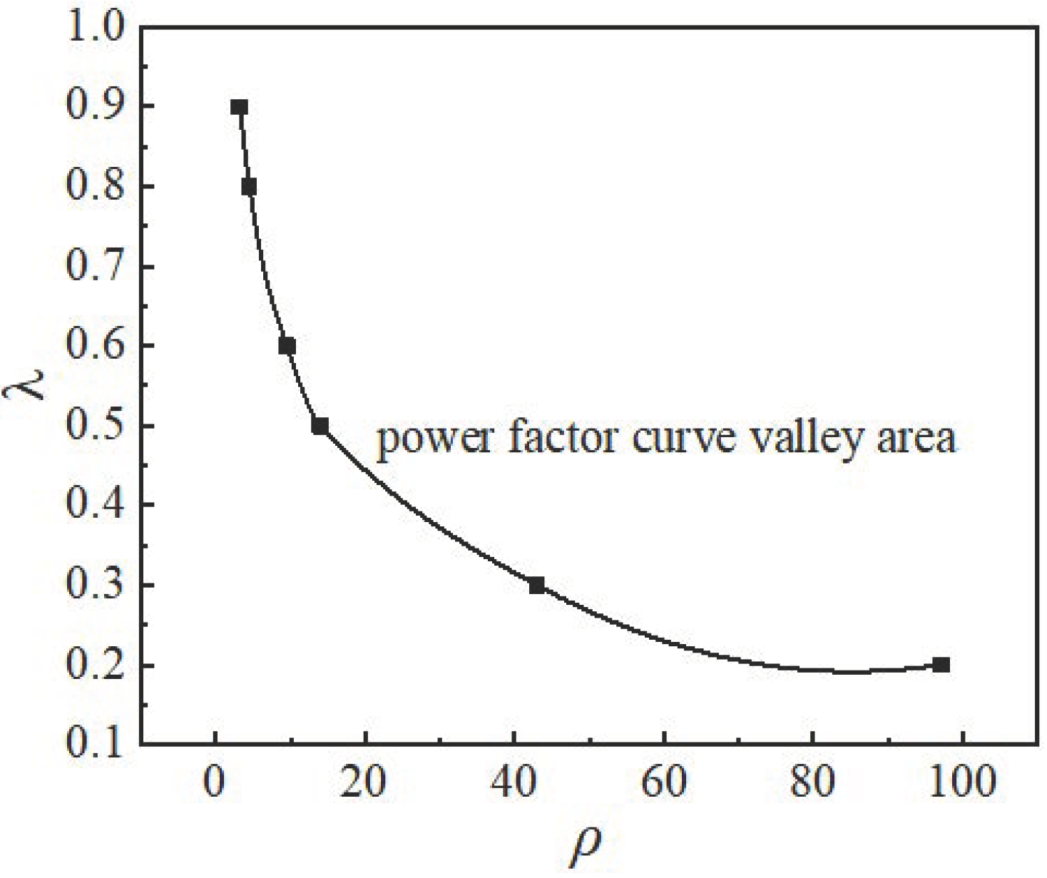
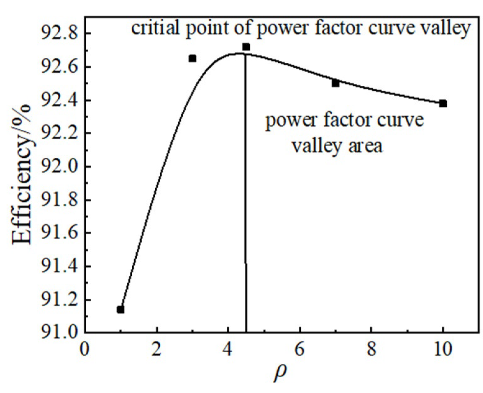
By linking the critical point of the power factor curve valley in the λ-ρ coordinate plane, the power factor curve valley area can be obtained. The parameter matching principles can be obtained as shown in Figure 11.

The dividing line is not a straight line, and the required ρ increases nonlinearly. The linear relationship is basically between λ = 0.6 and 0.9, and the required ρ value increases sharply in the interval less than 0.5. When the value is low, it is difficult to reach the state of power factor curve valley.

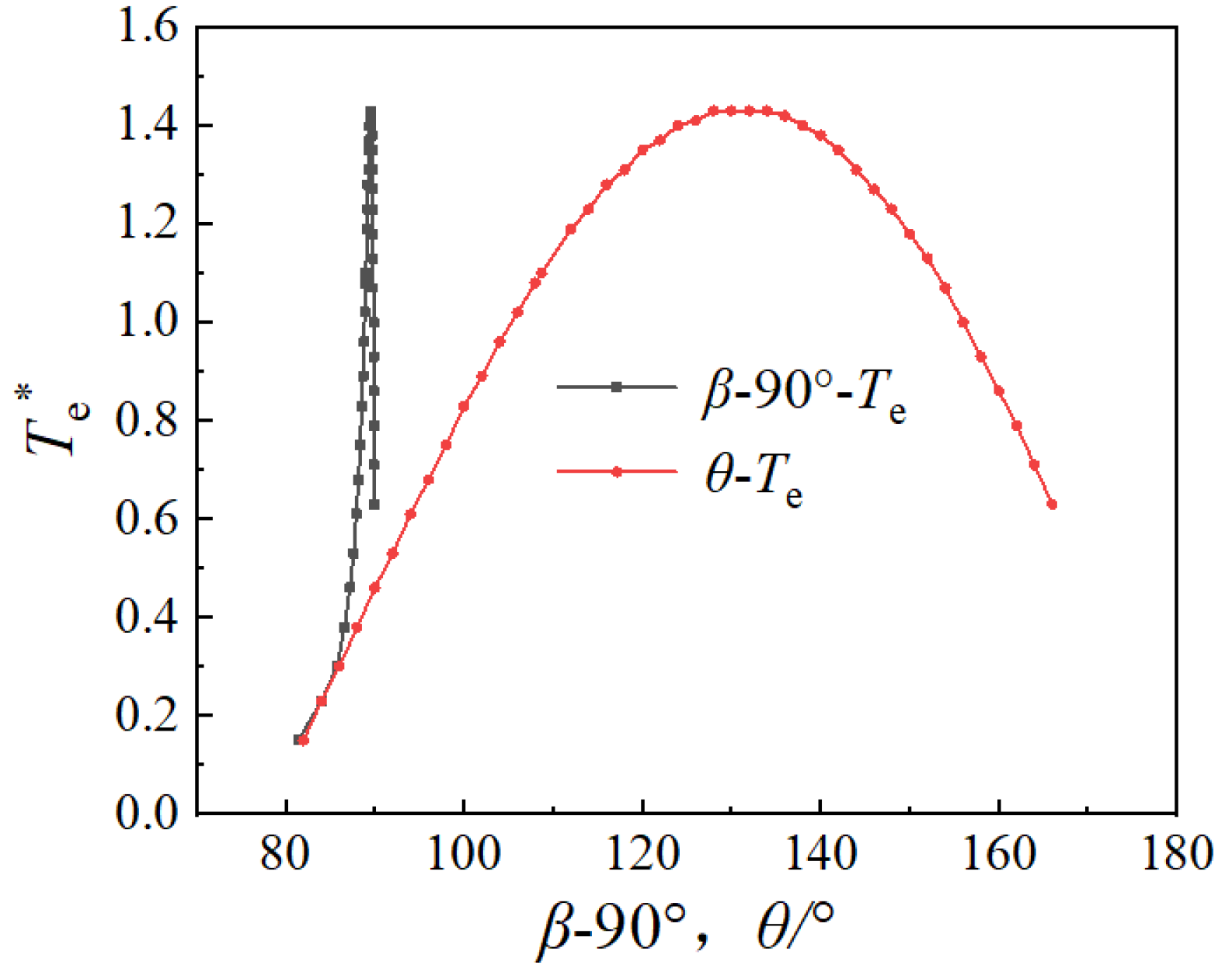
3.2. The Influence of Parameter Matching on the Load Rate of the Critical Point of Power Factor Curve Valley

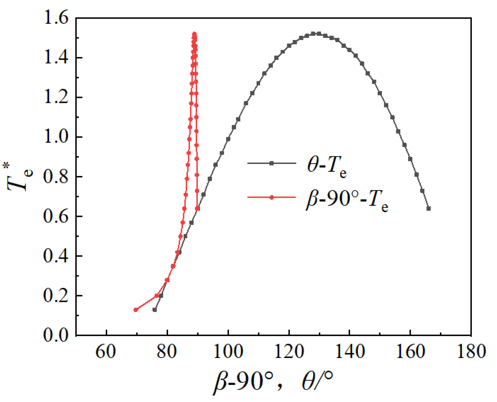
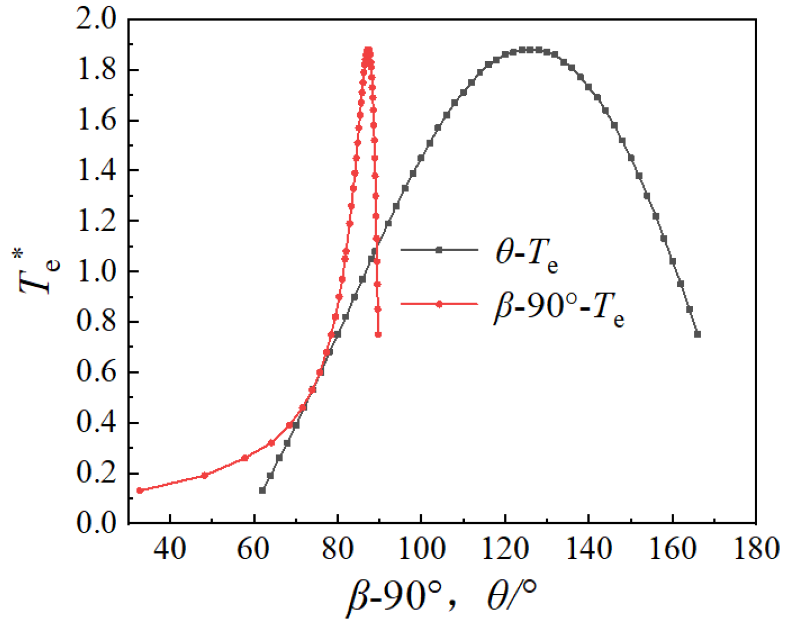
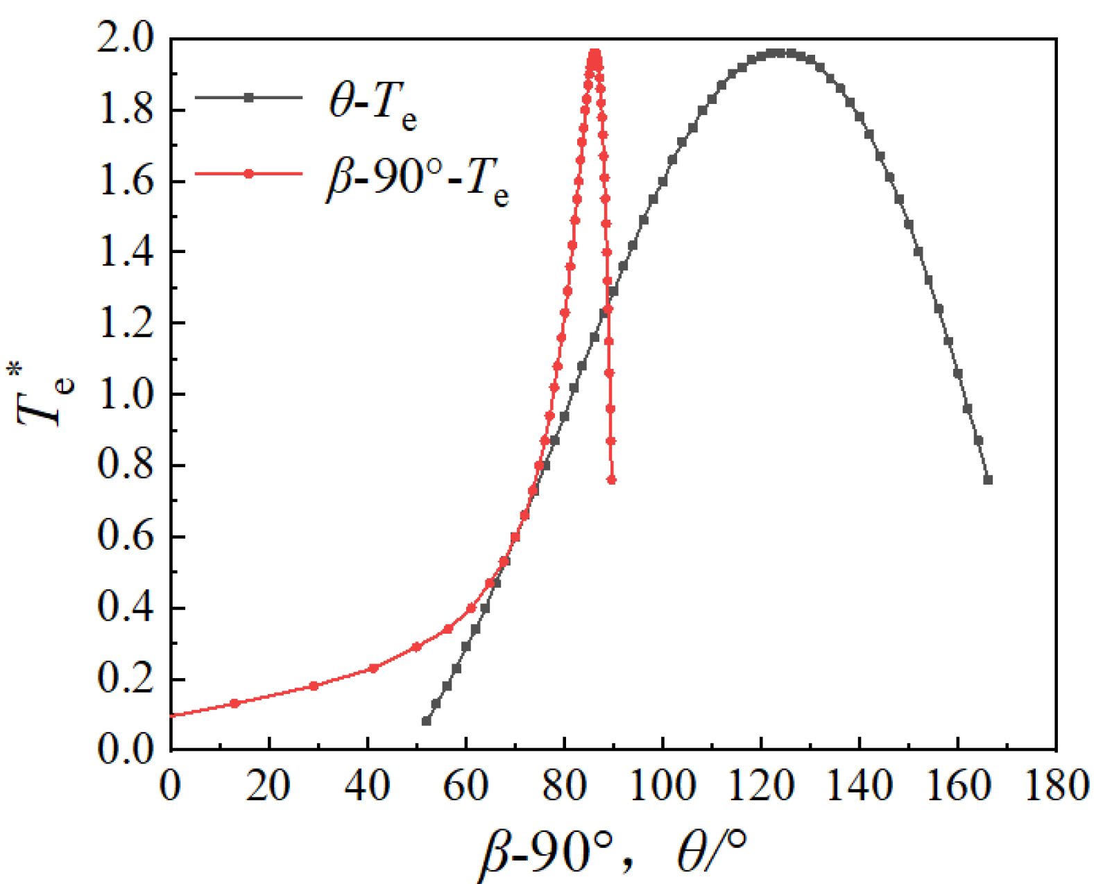
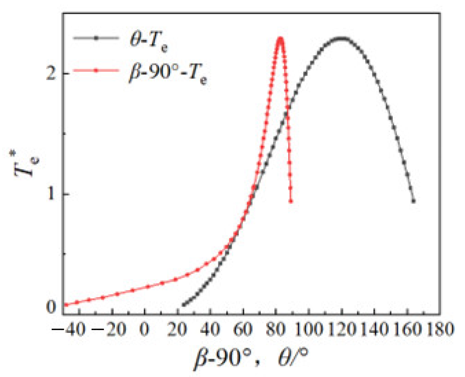
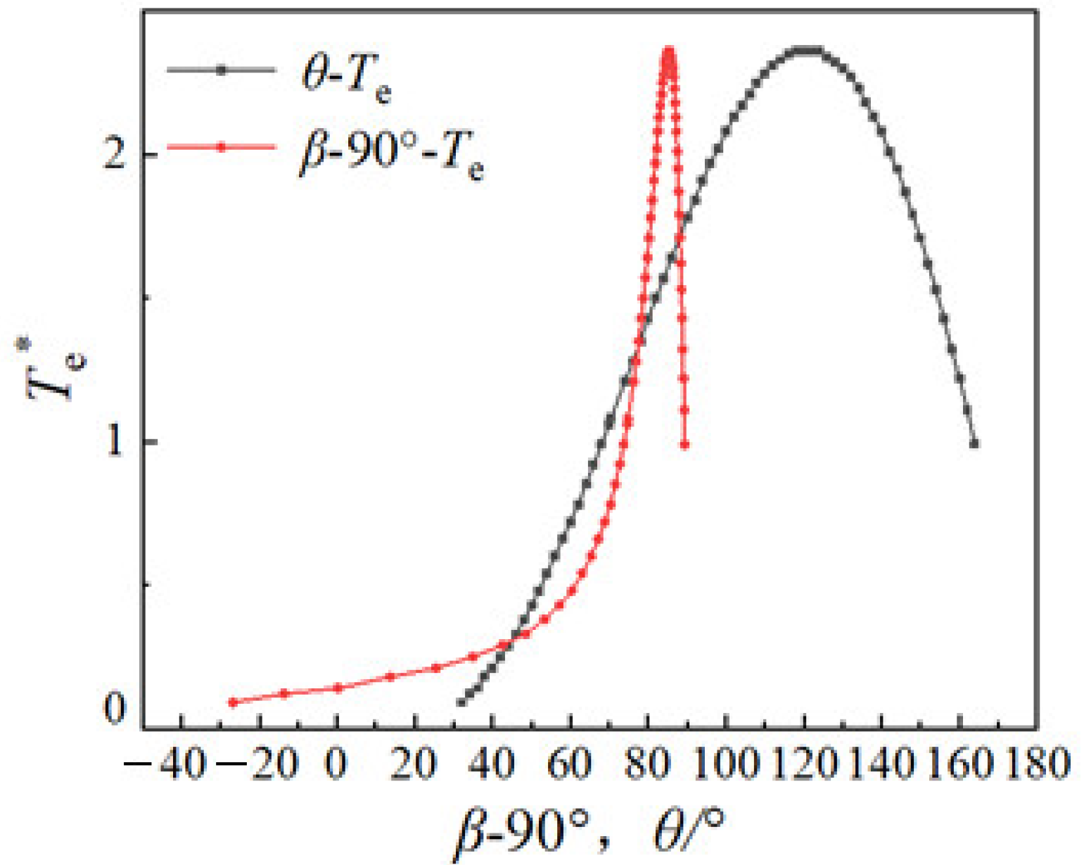
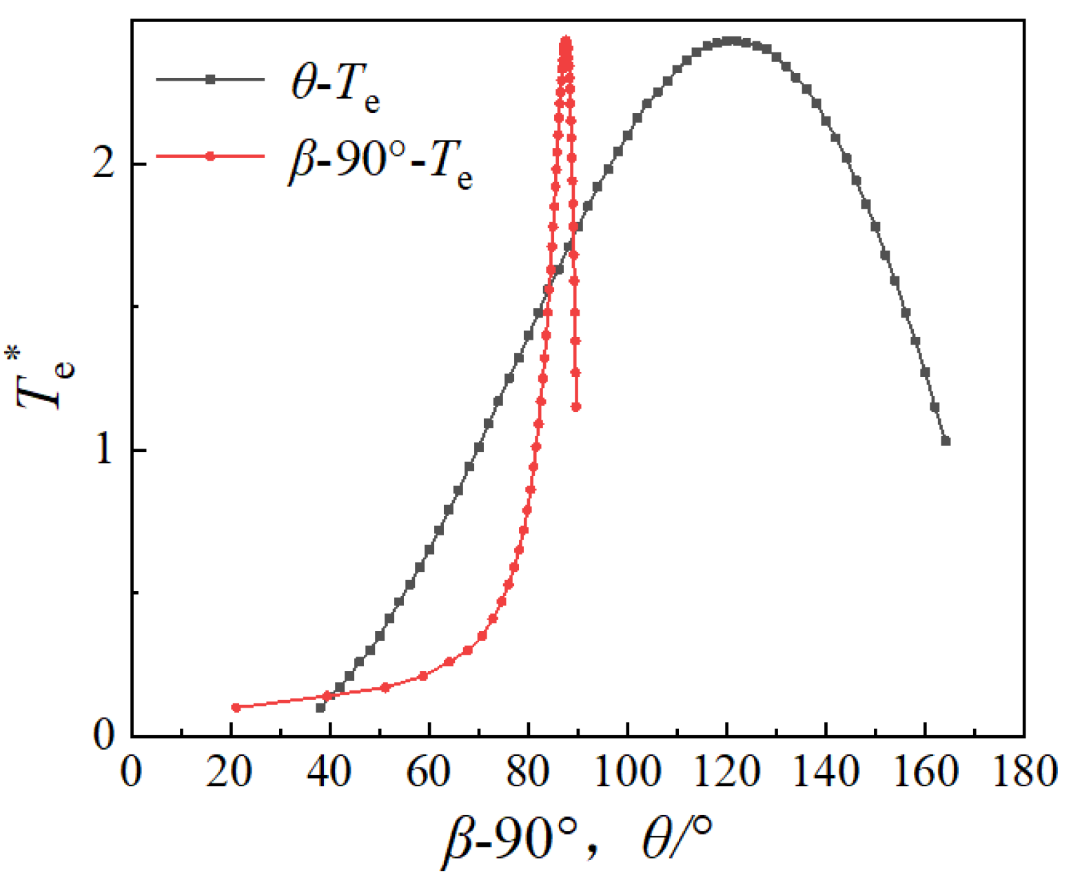
In the previous section, the conditions and parameter matching of power factor curve valley were analyzed. From Figure 10, it can be seen that the critical points of different states correspond to different θ values, indicating that the load rates are different. In order to obtain the principles, the torque curve in different states were calculated, and the β-T_e curve was moved to the left by 90° to make the relationship clearer, as shown in Figure 12, Figure 13, Figure 14, Figure 15 and Figure 16.

As can be seen from the above figures, the greater the value of λ, the greater the load rate corresponding to the critical point of the power factor curve valley. When the value of λ is small, the β-T_e curve is distributed in a smaller β angle range, while the torque range is relatively large. At the same time, the slope of the rising interval of the θ-T_e curve is relatively small, so the interval between two curves is smaller. When the value of λ is larger, the interval between two curves is larger, indicating that the interval of high power factor is larger. 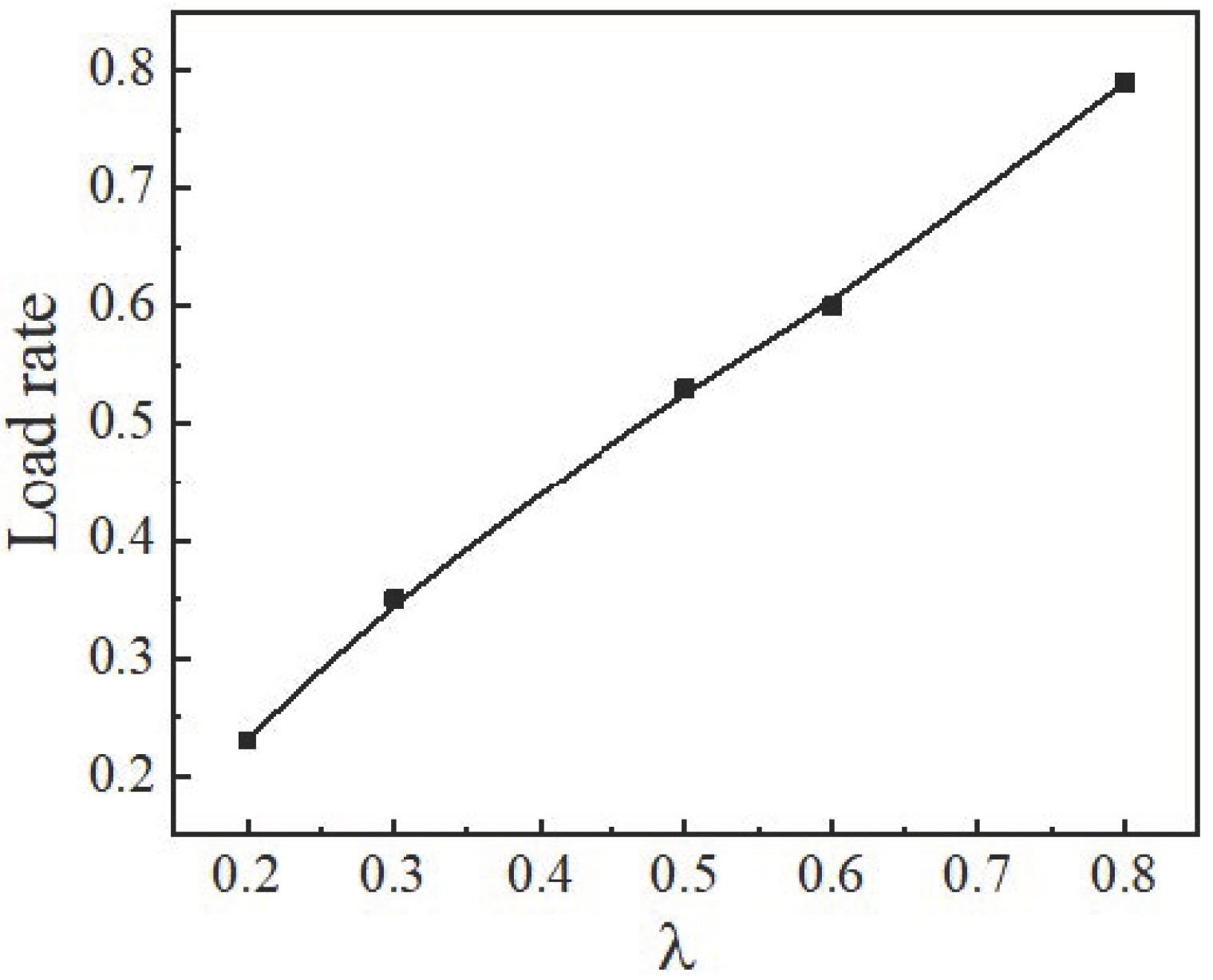The load rate curve corresponding to the critical point of the power factor curve valley under different λ is shown in Figure 17.

The load rate and value of λ basically change linearly, and the minimum current state at any load point can be obtained by selecting the reasonable parameters according to the curve.

3.3. Adjustment of Load Rate Corresponding to the Minimum Current Point

The load rate of the power factor curve valley can also be understood as the minimum current at a specific load rate. According to the analysis in the previous section, the minimum current under different load rates can be achieved under specific λ and ρ matching. This is a method of adjusting the load rate corresponding to the minimum current point. Its characteristic is to achieve the minimum current with the minimum ρ under each λ. The high load point requires a larger λ and a smaller ρ, and the low load point requires a smaller λ and a larger ρ. This can save the amount of permanent magnets. This is the most reasonable method in theory. However, its disadvantage is that low load requires a large ρ, which is difficult to achieve with the existing rotor manufacturing technology in engineering.

From the analysis, it can be seen that two minimum current load points are generated under the power factor curve valley. One point tends toward low load, and the other point tends toward high load. In this way, there can be a second method of adjusting the load rate corresponding to the minimum current point. The curves are shown in Figure 18 and Figure 19 when λ is 0.8.

The minimum current point gradually moves to low load as the salient ratio increases, so the minimum current at any load point can also be achieved. Compared with the first method, the second method can achieve the minimum current at the low load point with a smaller salient ratio. The disadvantage of this is that the load point current between two minimum points of current is large.

4. Influence of Power Factor Curve Valley of PMaSynRM on Whole Load Efficiency

The analysis of efficiency involves losses and needs to be targeted at specific research objects. A 5.5 kW motor was taken as an example for the present analysis.

4.1. The Influence of the Power Factor Curve Valley on the Efficiency of Load Rate Point

Different parameter matching can realize the power factor curve valley of any load point. In this state, further analysis is needed to determine whether the efficiency of the load point is optimal. λ = 0.5 and λ = 0.8 were selected to calculate the efficiency under different salient ratios. The load rate efficiency under the power factor curve valley is shown in Figure 20 and Figure 21.

As shown in Figure 20, the efficiency of the critical point of the power factor curve valley is not the highest. As the salient ratio increases, the efficiency changes from high to low.

As can be seen in Figure 21, the power factor curve valley occurs at a critical point with the highest efficiency, and the efficiency on both sides gradually decreases. The highest efficiency in different states is different. This is because the corresponding load point is the high load point when λ is 0.8. Here, copper loss accounts for a larger proportion of the total loss, and the magnitude of the current determines efficiency. Therefore, the power factor curve valley occurs at the critical point with the highest efficiency. The corresponding load point is the low load point when λ is 0.5. The copper loss accounts for a smaller proportion of the total loss, and the current cannot completely determine efficiency. The demagnetization field increases as the salient ratio decreases, the iron loss gradually decreases, and the efficiency gradually increases. By combining the loss rate of each load point, a reasonable design of motor parameters can obtain optimal efficiency of any load.

4.2. The Influence of the Corresponding Load Rate Point of Power Factor Curve Valley on Whole Load Efficiency

Although a reasonable design of motor parameters can obtain optimal efficiency of any load, the effect of the size of the high-efficiency zone in the whole load range needs further research. The conditions of λ = 0.5 and λ = 0.8 were again selected for analysis. The power factor and efficiency of the whole load were calculated and are shown in Figure 22, Figure 23 and Figure 24.

Compared with the state of λ = 0.5, the power factor of low load is higher and the power factor of high load is lower, as shown in Figure 22. Compared with the state of λ = 0.5, the low load efficiency is high, and the high load efficiency is low, as shown in Figure 23 and Figure 24. The copper loss accounts for a large proportion of total loss in the high load area. The current state of λ = 0.8 is small and has high efficiency. The current of λ = 0.5 in the low load area is small and has high efficiency, but the copper loss is small. Therefore, the low load efficiency difference between the two states is less than that for high load efficiency. As can be seen, the larger the λ, the larger the range for high efficiency, and the smaller the λ, the higher the efficiency range for low load.

5. Prototype Test

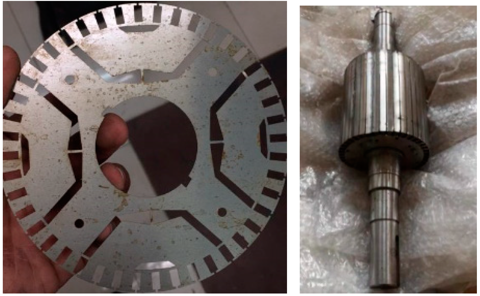
A 5.5 kW PMaSynRM was designed and manufactured. The parameters of the motor are shown in

Table 1. Main parameters of the prototype.

Parameters	Value
Power	5.5 kW
Rated speed	1500 r/min
Poles	4
Inner/outer diameter of stator	210 mm/136 mm
Stator slots	36
Air gap	0.5 mm
Core length	145 mm
Phase resistance	0.559 Ω
d-axis inductance	41.1 mH
q-axis inductance	127.8 mH
Flux linkage of the permanent magnet	0.723 Wb
Leakage stator inductance	5.54 mH
Rotor leakage inductances in q-axis referring to the stator side	3.06 mH
Rotor leakage inductances in d-axis referring to the stator side	3.06 mH
Rotor resistance in d-axis	0.740 Ω
Rotor resistance in q-axis	0.740 Ω
Moment of inertia	0.05 kg·m2
Maximum moment of inertia with a static load moment torque to the rated value	3.5 kg·m2
Magnet grade	N38SH
Electric steel grade	35W270

, and the structure of the rotor is shown in Figure 25. The inductance of the prototype was tested as shown in Figure 26. The d-axis inductance was 41.1 mH, the q-axis inductance was 127.8 mH, and the salient pole rate of the motor was 3.11.

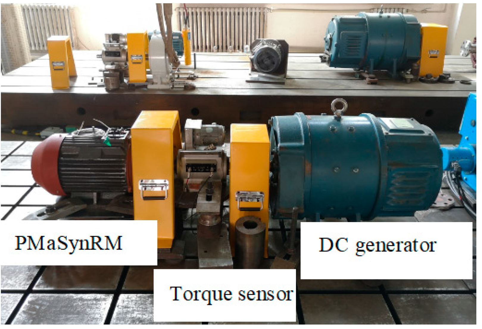
The rated phase voltage of the prototype was 220 V, and the back-EMF was 160.5 V by experimental test. λ and ρ were not on the curve of the critical point of the power factor curve valley discussed above, and the back-EMF and ρ could not be changed after the prototype was produced. In order to verify the correctness of the above conclusions, the input voltage was only changed for testing. According to the previous curve, when input voltage is adjusted to 174.3 V, the motor is in a critical state of the power factor curve valley. 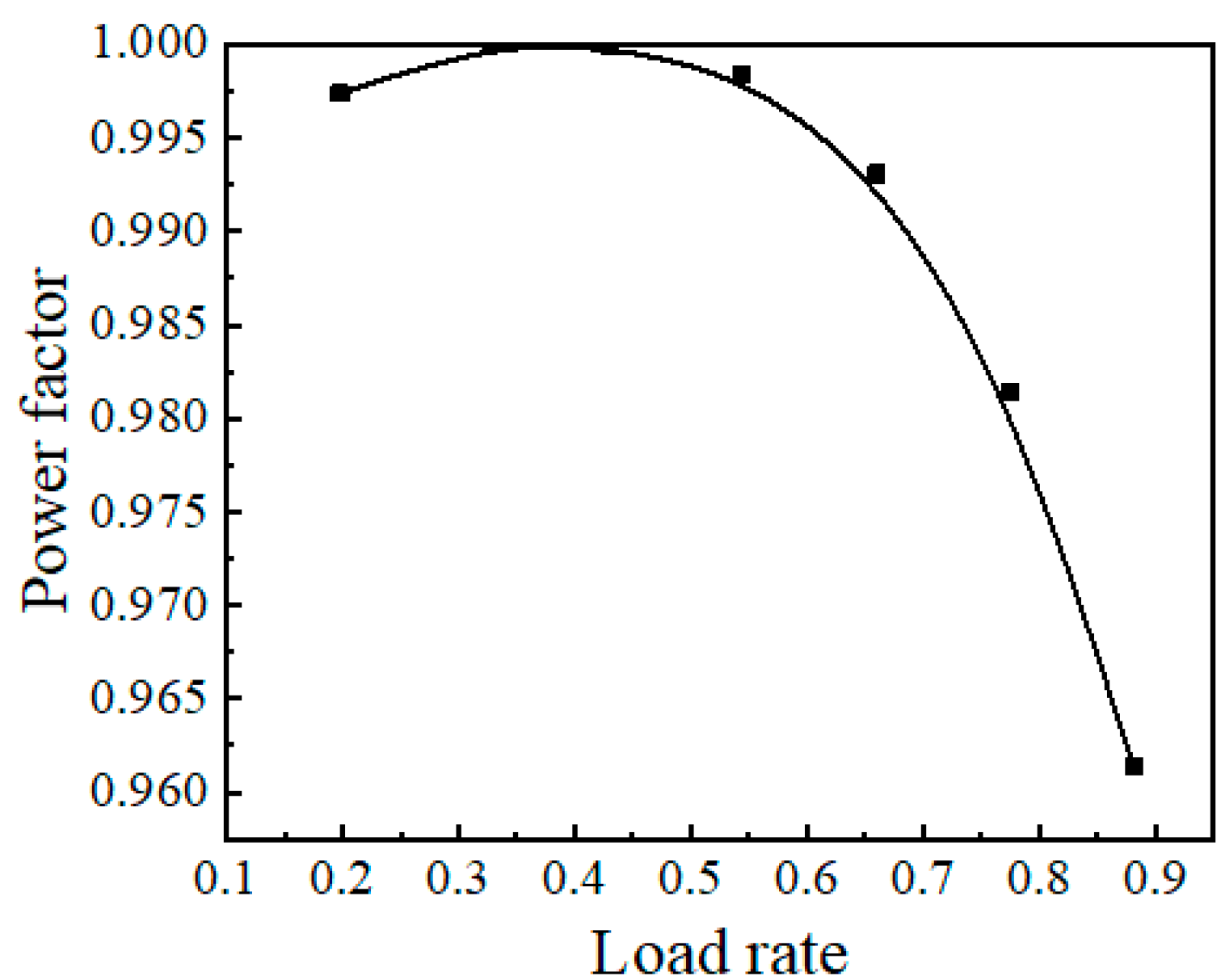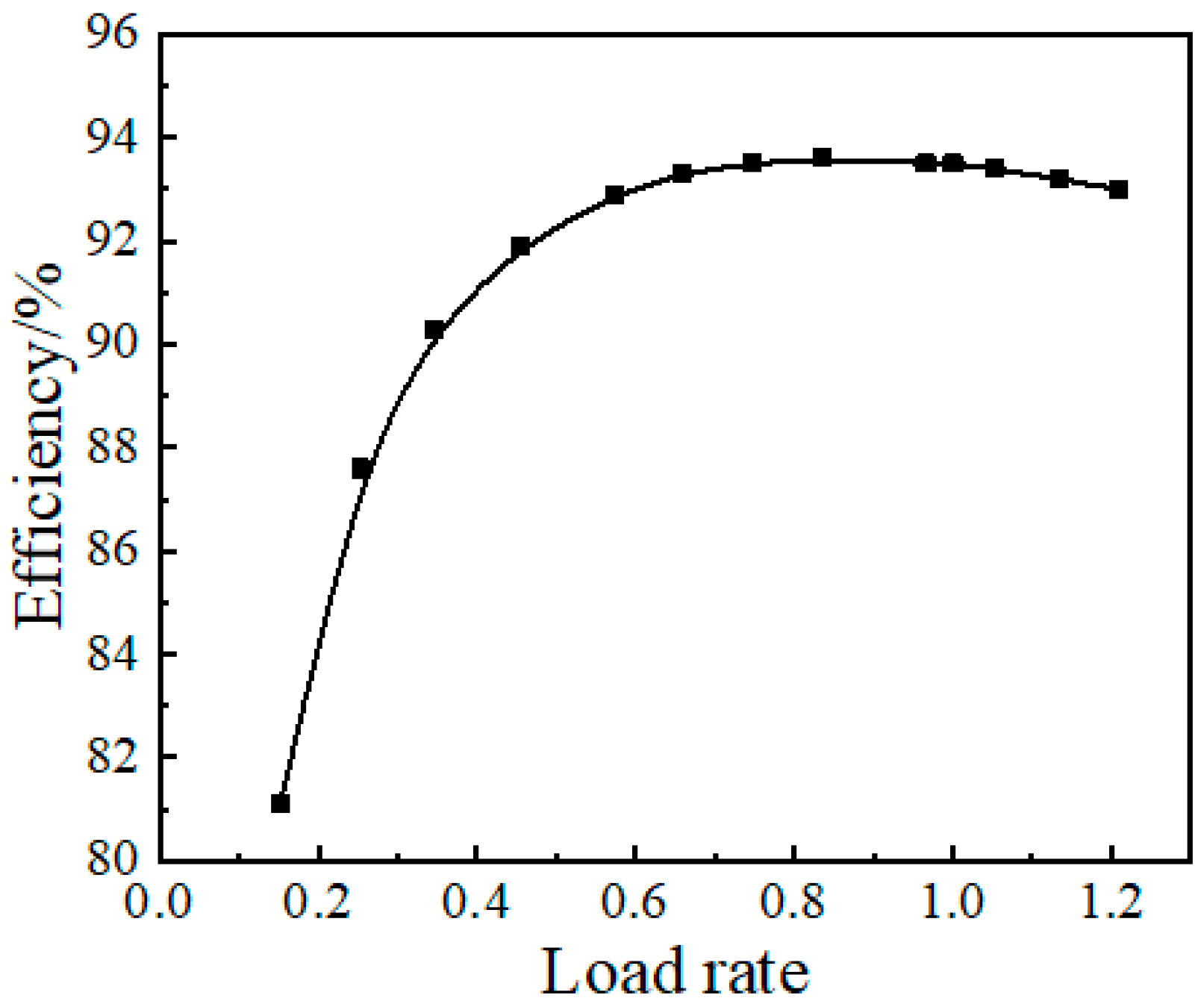The input voltage was adjusted to 174.3 V, and the power factor was tested as shown in Figure 27. The PMaSynRM was used as the tested motor linked to a torque sensor, and the load motor was a DC generator. The test power factor curve is shown in Figure 28, and the efficiency curve is shown in Figure 29.

The test results showed that, when the power factor reached 1, the load rate was between 0.3 and 0.4, which is the critical state of the power factor curve valley.

6. Conclusions

From the LSPMaSynRM mathematical model, the principle of the power factor curve valley was derived, and its parameter matching principle was analyzed. Then, the characteristics of the corresponding load rate and the influence on whole load efficiency were further analyzed. The conclusion reached in this study is not confined to any specific rotor structure. As long as the parameter matching conforms to the analysis carried out here, the corresponding power factor characteristics can be obtained, thus providing a certain theoretical basis for the detection and judgment of the motor running state. The conclusions are as follows:

(1).

The principle of the power factor curve valley of LSPMaSynRM is that the matching of specific motor parameters causes the torque curve to deform, and a valley is generated by two intersection points when two torque curves are in the stable operating range. The parameter matching relationship is shown in Figure 11, λ is basically a linear relationship between 0.6 and 0.9, and the required ρ value increases sharply in an interval of less than 0.5.

(2).

The load rate at the critical point of the power factor curve valley is basically linear to λ and increases with increasing λ.

(3).

A reasonable design of motor parameters can obtain the minimum current for any load. In the critical state of power factor curve valley of different parameter matching, the larger the λ, the larger the high-efficiency range and the higher the efficiency of the high load, whereas the smaller the λ, the higher the efficiency of the low load, Shengnan Wu, Zhanyang Yu and Lihui Chen.