
Power Transformer Diagnosis Based on Dissolved Gases Analysis and Copula Function


1
State Grid Jiangsu Electric Power Co., Ltd. Research Institute, Nanjing 211103, China
2
Jiangsu Key Laboratory of New Energy Generation and Power Conversion, Nanjing University of Aeronautics and Astronautics, Nanjing 211106, China
*
Author to whom correspondence should be addressed.
Energies 2022, 15(12), 4192; https://0-doi-org.brum.beds.ac.uk/10.3390/en15124192
Submission received: 28 April 2022
/
Revised: 24 May 2022
/
Accepted: 26 May 2022
/
Published: 7 June 2022
(This article belongs to the Special Issue Frontiers in Advanced Power Equipment and Research in Condition Diagnostic and Sensing)
Abstract
:The traditional DGA (Dissolved Gas Analysis) diagnosis method does not consider the dependence between fault characteristic gases and uses the relationship between gas ratio coding and fault type to make the decision. As a tool of the dependence mechanism between variables, a copula function can effectively analyze the correlation between variables when it cannot determine whether the linear correlation coefficient can correctly measure the correlation between variable relationships. In this paper, the edge variable of a copula function is selected from the fault characteristic gas of a transformer, and the distribution type of the edge variable is fitted at the same time. Then, Bayesian estimation with the Gaussian residual likelihood function is used to fit the parameters of a copula function and a copula function is selected to describe the optimal dependence of the fault characteristic gas of transformer. The relationship between a copula function and the state of transformer is studied. The results show that the copula function boundary with hydrocarbon gas as edge variable can divide the transformer as healthy or defective state. When the cumulative distribution probability (CDF) value of the dissolved gas in the oil in the copula function is close to 0.8, the fluctuation of its gas concentration leads to a sharp change in the probability. Therefore, the analysis of dissolved gas in oil based on a copula function can be used as a powerful technical solution for oil-immersed power transformer fault diagnosis.
1. Introduction
Oil-immersed transformers are key equipment in power systems, and the transformer failure rate is an important indicator for assessing the reliability, which can provide an important basis for developing scheduling operation, maintenance plans, and grid planning. Since insulating oil is prone to decompose into a variety of small molecule hydrocarbon gases under abnormal operating conditions, dissolved gas analysis (DGA) in transformer oil has become a common and effective method for fault diagnosis of oil-immersed transformers to obtain insight into the internal state of transformers [1,2].
The methods to interpret DGA can be classified into traditional gas ratio methods [1,3,4], intelligent algorithms represented by expert systems and supervised learning [5,6], and deep-learning-based models [7,8,9]. Although the traditional gas ratio method can detect latent transformer faults more accurately and prevent further deterioration of transformer faults, it suffers from missing codes and an increased rate of misclassification within the fault boundary [3,4].
In addition, in response to the deficiency of the traditional ratio method, which does not have adaptive learning capability itself, theories, such as artificial neural networks [10,11], support vector machines [12,13], and fuzzy theory [14,15,16], began to be applied in the field of transformer fault diagnosis to improve the accuracy of fault diagnosis. However, the performance of neural networks depends on the network structure of artificial neural networks and the gradient descent algorithm for error reduction.
Different application scenarios require the selection of different neural network structures and gradient descent algorithms, which require the staff developing the models to have a rich prior knowledge. In particular, the selection of kernel functions and the selection of multiclassification structures, such as “one-to-many”, “one-to-one”, and “directed acyclic graph”, in multiclassification support vector machines requires extensive a priori knowledge in different application scenarios [17].
Thus, it is difficult to guarantee the wide application of the optimization ideas of the analysis and diagnosis model of dissolved gas in oil. The advantage of deep-learning methods applied in the field of transformer fault diagnosis is that the complex neural network structure can approximate the complex mapping relationship between oil chromatography data and transformer fault states, thus, it helps to improve the accuracy in fault diagnosis.
The deep recursive belief networks are established for the time-domain correlation of oil chromatography data, and adaptive delay networks based on the autocorrelation principle are established for transformer state prediction and fault diagnosis [18,19]. Nevertheless, the continuous expansion of neural network size and exponential increase of degrees of freedom bring difficulties to the training of deep network models, and there is no standard correlation index to measure the generalization performance and overfitting of deep networks.
Copula functions have systematic theoretical support in correlation analysis between variables, parameter fitting, and function type selection, and have been widely used in financial risk and hydrological analysis [20], statistical analysis [21] and signal processing [22]. For the risk analysis of transformer failure, the internal state of transformer is closely related to the concentration of dissolved gases in oil, and there is a high correlation between various hydrocarbon gases generated by the decomposition of insulating oil.
Therefore, the correlation between the state of transformer and the joint distribution of copula functions can be studied by establishing a copula function with dissolved gas in oil as the variable. In addition, the diversity of copula function forms makes it convenient to depict both nonlinear, asymmetric, top-tailed dependence, bottom-tailed dependence, and mixed dependence relationships between dissolved gases in oil for dependence analysis [23].
Copula functions are free from the dependence of traditional machine-learning methods relying on a priori knowledge in terms of model topology and gradient optimization. In addition, the copula function has a very simple mathematical relationship with the rank correlation coefficient, which greatly simplifies the computational process and improves efficiency. Not only is it easy to establish the corresponding mathematical model but also this can reflect the nonlinear relationship between random variables to avoid the impact of random fluctuations and guarantee robustness.
With the above consideration, it is proposed to use the rank correlation coefficient to describe the correlation of random variables via selecting the marginal variables of the copula function from the dissolved gases in transformer oil. Afterwards, the distribution type of marginal variables is fitted, and then the most suitable copula function type is confirmed on the basis of goodness-of-fit test. At last, the copula model is demonstrated through the actual data of dissolved gas in transformer oil.
2. Copula Function and Common Factor Analysis
To deal with the DGA data from power transformers, copula function and common factor analysis are necessary.
2.1. Copula Function
The formulation of Sklar’s theorem laid the foundation of copula theory. The copula function can be used to describe the dependence connection between dissolved gases in oil, and represent the joint probability distribution of dissolved gases in oil as the “connection” of their respective marginal distributions, which is a powerful tool to construct the joint distribution of dissolved gases in oil. The copula function has two advantages. On one hand, a copula is able to determine the dependence type, which is invariant under the monotonic incremental transformation of dissolved gases in oil. On the other hand, the copula function is used as a starting point for constructing two-dimensional distribution clusters and stochastic simulations and can be used for correlation analysis studies between dissolved gases in oil.
Sklar’s theorem assumes that F is the joint probability distribution function of random variables x1, x2,…, xn of marginal distributions F1, F2,…, Fn, then there is a copula function C, for any X ϵ R:
Sklar’s theorem proves that if F1, F2,…, Fn are continuous, then C is unique, and the copula function C can be derived from Equation (1):
According to Sklar’s theorem, when the marginal distribution of each component of dissolved gas in transformer oil and the suitable copula function are determined, the joint probability distribution of dissolved gas in transformer oil can be obtained. Although the content of dissolved gas in oil under fault is not a random event, the correspondence between its content and the internal state of transformer itself has randomness.
The correspondence between its content and the internal state of the transformer itself shows a randomness in nature; however, the correlation between this randomness and the content of dissolved gas in the oil has a certain law. A copula function plays an important role in practical application as a risk tool for correlation analysis. The modeling process of transformer fault risk analysis is divided into two main steps: Step 1, constructing the marginal distribution of each component of dissolved gases in oil; Step 2, choosing a suitable copula function and determining its parameters as a tool to describe the correlation structure of transformer states.
A copula function can be divided into different types according to the construction methods, the common types of copula function distribution are Gumbel copula, Clayton copula, and Frank copula. Among them, the Gumbel copula function is more sensitive to the change of variables in the upper tail of the distribution, which is suitable to capture the change related to the upper tail. Its form is as follows.
In the above equation, u and v are the cumulative distribution probability of dissolved gas in oil, θ is the parameter of Gumbel copula function.
The density function of the binary Clayton copula also has asymmetric tails. Unlike the Gumbel copula function, the Clayton copula function is more sensitive to changes in the lower tails of the distribution. It can capture the changes associated with the lower tails very well. Its density function image is L-shaped with a low upper tail and a high lower tail, which takes the following form.
Frank copula’s density function has symmetry and can capture the symmetric tail correlation between random variables. Similar to the bivariate normal copula function, its tail is asymptotically independent, and the form is as follows:
The parameter θ in the function directly reflects the dependence of the variables of the copula function, that is, the correlation between the dissolved gases in the oil. But its numerical range is related to the type of the copula function, and the correlation between the dissolved gases in the oil of different copula functions cannot be uniformly measured merely according to the parameter θ. Therefore, the rank correlation coefficient description is used to measure the correlation, and its form is as follows:
The calculation of the rank correlation coefficient needs to arrange the random variables from low to high, and then calculate the product-rank correlation coefficient of their respective ranks to obtain the monotonic relationship between the random variables. In order to convert the marginal distribution to the corresponding rank, the cumulative distribution function F of the random variable is required, and the uniform distribution random variable is generated by the cumulative distribution function transformation.
2.2. Common Factor Analysis
Since transformer fault information can be inferred from at least five transformer fault characteristic gases (hydrogen, methane, ethane, ethylene, and acetylene), it is particularly important to select appropriate marginal distribution variables to construct a joint distribution function to describe transformer fault information.
In order to solve the selection problem of dissolved gases in oil, this paper adopts the method of factor analysis, instead of several combinations in the traditional ratio method. The calculation involved in factor analysis is very similar to that of principal component analysis; however, principal component analysis divides variance into different orthogonal components, while factor analysis divides variance into different components. Cause factor, the calculation of eigenvalues in factor analysis can only start from the correlation coefficient matrix, and the principal components must be converted into factors. Factor analysis has a definite model, and the observation data is decomposed into three parts: common factor, special factor, and error in the model.
Therefore, the basic steps of factor analysis can be divided as four steps. First, it is necessary to find the eigenvalues of the dissolved gas correlation coefficient matrix R in the oil (in order of magnitude) and its corresponding eigenvectors. Then, it is time to take the first k eigenvalues to make the cumulative variance contribution rate exceed the set threshold, and give the eigenvectors corresponding to the first k eigenvalues. Afterwards, the factor loading matrix A is obtained. Finally, the load matrix A can be orthogonally rotated so that the sum of the variances of the obtained matrix is the largest.
Before performing factor analysis, it is necessary to perform KMO (Kaiser–Meyer–Olkin) test and Bartlett sphericity test for dissolved gas in oil to verify that the results of factor analysis can represent most of the original data. The KMO test statistic is an index used to compare simple and partial correlation coefficients between variables.
The calculation of the KMO test involves the correlation matrix R (correlation matrix) and the reflection image correlation matrix Q (anti-image correlation matrix). The reflection image correlation matrix Q can be calculated by the inverse matrix of the correlation matrix R:
In the above formula, diagR−1 sets other off-diagonal elements of the inverse matrix of the correlation matrix R to 0, and the KMO statistic is:
In the formula, rij and qij are the correlation matrix R and the ith row and jth column elements of the image correlation matrix, and the KMO statistic is between 0 and 1. When the sum of squares of correlation coefficients among all variables is much larger than the sum of squares of partial correlation coefficients, the closer the KMO value is to 1, the stronger the correlation between variables, the more suitable the original variables are for factor analysis. This is vice versa when the sum of squares of the simple correlation coefficients is close to 0.
Bartlett’s sphericity test is a hypothesis method used to test the correlation between variables in a correlation matrix—that is, to test whether every variable is independent to each other. According to the Bartlett’s sphericity test, if the null hypothesis is rejected, factor analysis can be done. If the null hypothesis is not rejected, the variables may be independent to each other, which is not suitable for factor analysis. The null hypothesis H0 and the alternative hypothesis Ha of the Bartlett sphericity test are that the variances of the k samples are equal and that there are at least one group of samples with unequal variances, respectively. Its statistic can be calculated by the following formula:
In the above formula, N is the sum of the sample data, k is the sample size, and Ni is the data size of the i-th sample, the variance of the i-th sample, is the combined variance of the samples, which is defined as:
3. Copula Function Selection and Parameter Fitting
The selection of copula function and its fitting are the critical step to understand the distribution and contribution of fault gases.
3.1. Bayesian Estimation of θ
Bayesian estimation takes the parameter θ as an unknown random variable, and updates the parameters of the assumed prior probability according to the observed data. It is often used for model inference and uncertainty quantification. First, the posterior distribution of the model parameters is estimated according to the following formula:
where θ is the parameter of the dissolved gas distribution in the oil, is a set of data composed of the dissolved gas in the oil, and and represents the prior and posterior distributions of the unknown model parameters, respectively. When the prior distribution of the model parameters is unknown, the prior distribution of model parameters is assumed to be uniform. This paper assumes that the residuals of the observed data and the real data are independent of each other and obey a Gaussian distribution with the mean of 0. Then, the likelihood function is:
In which is the observed data, is the real data of the model under the parameter , and σ is the standard deviation of the error between the observed data and the real data. Under the premise of a given Gaussian distribution, σ can be calculated by the following formula:
The parameter of the copula function reflects the correlation of the input variables, which directly affects the quality of the copula function in fitting dissolved gases in oil. The choice plays on the strengths of domain knowledge, and its posterior distribution can quantify uncertainty about the model.
3.2. Goodness of Fitting
After fitting the parameters of different copula functions through Bayesian estimation, root mean square error (RMSE) and Nash coefficient (NSE), are used in this paper. The two indices are helpful to describe goodness of fitting the dissolved gas in transformer oil and determine the best type of copula function.
Compared with low-complexity models, high-complexity models can often achieve better fitting results for the same observation data. However, excessive model complexity also leads to the shortcomings of over-fitting. In this regard, NSE and RMSE are different from the Akaike Information Criterion (AIC) and the Bayesian Information Criterion (BIC), the model complexity is not concerned, and the forms are as follows:
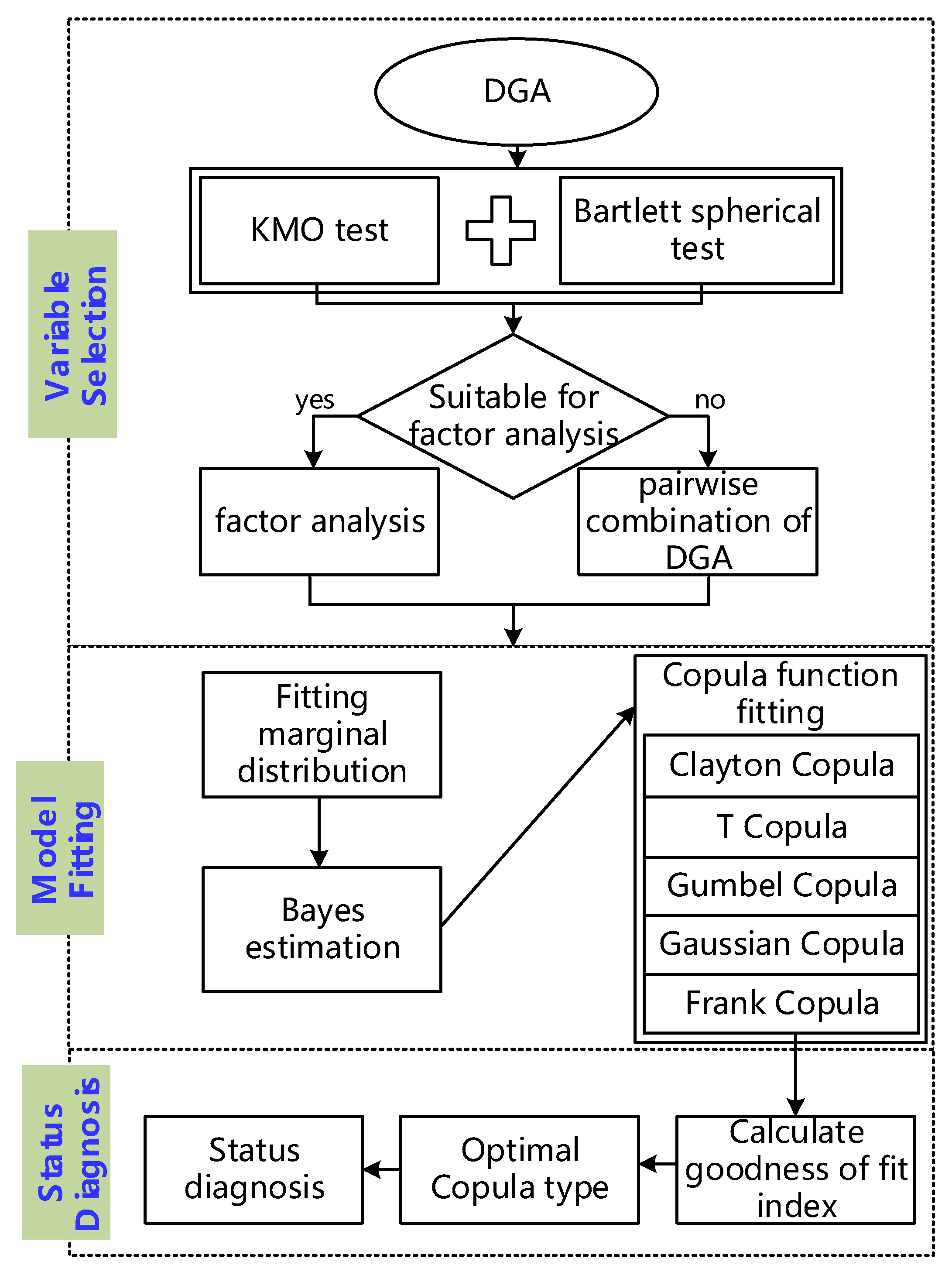
The indicators of the goodness of fitting, RMSE and NSE, directly reflect the error between the model fitting results and the observed data. They provide a standard for the selection of the subsequent copula function type. To sum up, the data processing and diagnosis flow chart of dissolved gas in oil based on a copula function is shown in Figure 1.
4. Study Cases
The framework of copula-function-based technique is established, and field DGA data and cases are necessary to evaluate the strategy.
4.1. Factor Analysis of Dissolved Gas in Oil
In general, two dataset is classified and organized. The first dataset is sourced from the live detection of medium and high temperature overheat fault transformers, provided by a power company with a total of 2073 pieces of data from 27 transformers. The second part of the data is copied from the same power company; however, for the normal transformer live detection, a total of 4691 pieces of data from 76 transformers are used. Of these, most transformers make use of KI 25X/45X, meeting the standards of IEC 60296-2003. In total, the relevant data and status labels of 103 transformers are identified.
The copula functions in this paper are selected as binary copula functions, including the Frank copula, Gaussian copula, T copula, Gumbel copula, and Clayton copula. The common factor loading analysis corresponds to the number of variables in copula function. Thus, the number of loading common factors in this manuscript is set as 2, as shown in Table 1.
After inspection, the contribution rates of common factor loading 1 and common factor loading 2 are 35.44% and 30.21%, respectively. The total contribution rate of the two common factor loadings does not exceed 70%, and a great deal of information is lost, as shown in Table 1. The KMO test and Bartlett sphere test are required for dissolved gases in transformer oil. The KMO value of the original data is 0.3951, which is much lower than 1 and is not suitable for factor analysis. The original data shown by the Bartlett sphericity test results accepts the null hypothesis. With the results of the KMO test and the Bartlett sphericity test, the dissolved gas in the oil is not suitable for factor analysis.
4.2. Marginal Distribution Fitting
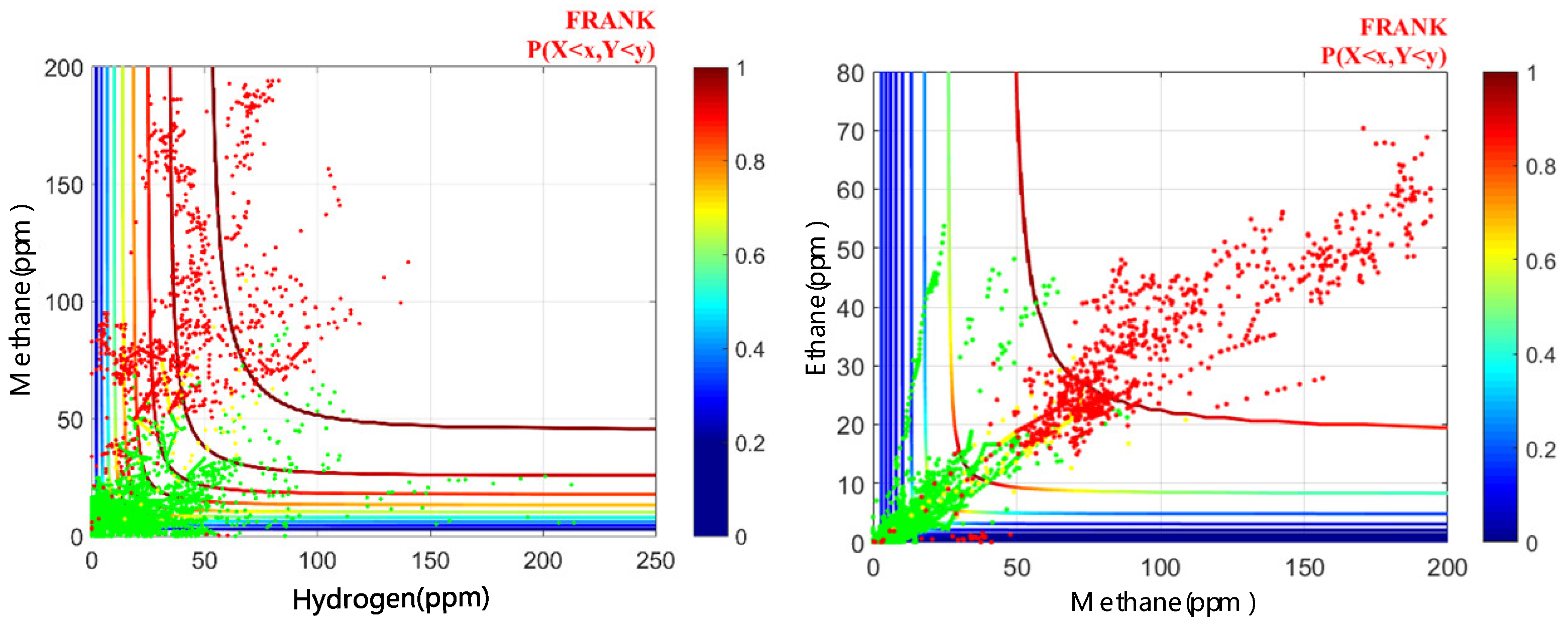
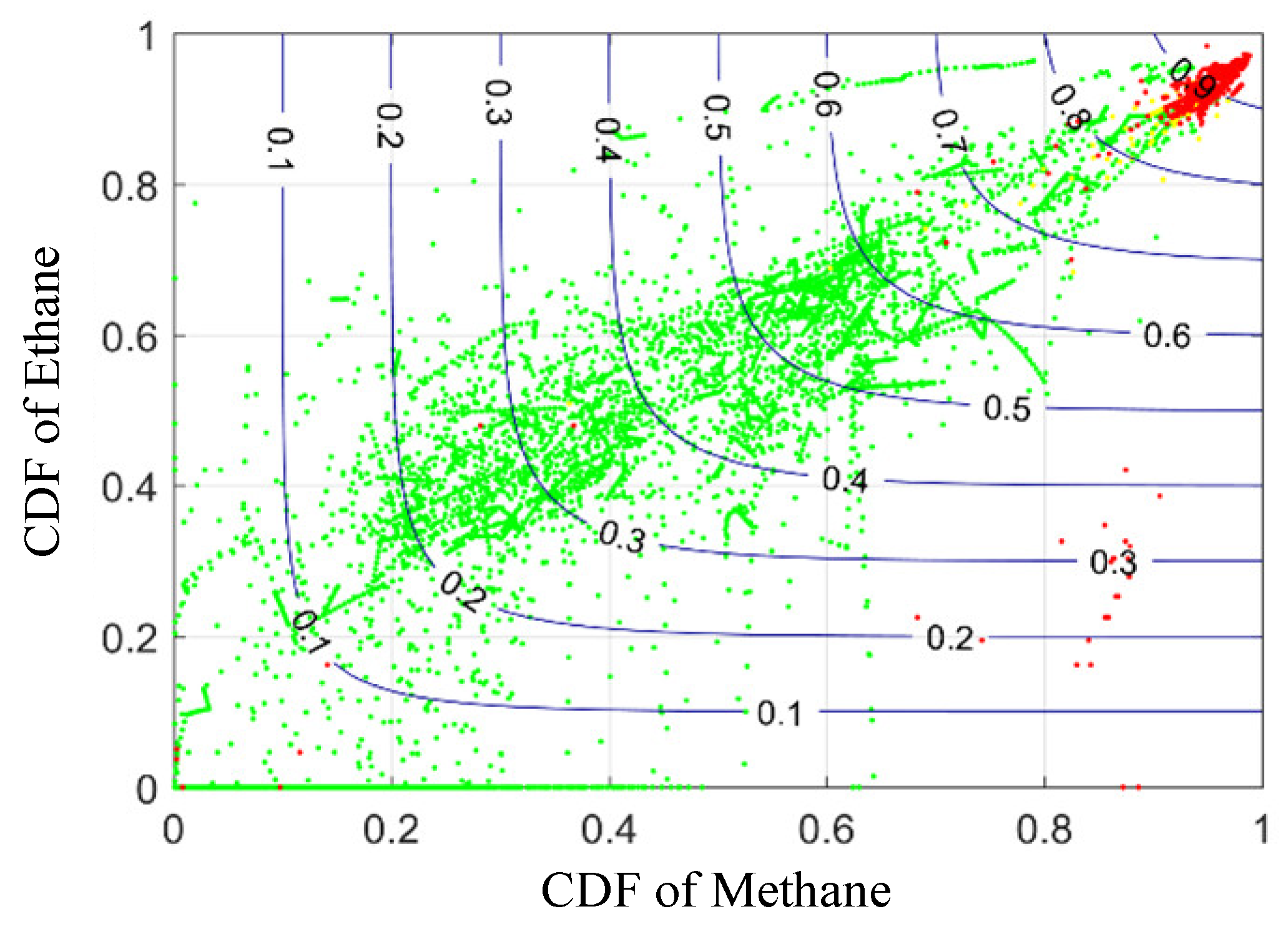
Since the low-dimensional dissolved gas in transformer oil cannot be extracted as the input variable of the copula function through factor analysis. The copula function selected in this paper is a binary copula function, the number of independent variables is limited to 2, and only two of the fault characteristic gases can be used. The two combinations are used as the input for the copula function. In order to utilize the cumulative distribution probability (CDF) results of the copula function, the distribution of transformer states can only be observed in the joint distribution of the existing combination variables, as shown in Figure 2.
In this work, 28 copula joint distribution functions for the combination of gas variables with comprehensive fault characteristics have been carried out. Among them, the transformer state data in the copula function distribution of the combination of hydrocarbon gas variables can be divided by the CDF boundary, and the state of the transformer in the copula joint distribution function cannot be demarcated by the CDF with the combination of hydrogen and other gases. It can be seen that when the correlation between the input variables is strong, the CDF result of the copula function can effectively judge the transformer state.
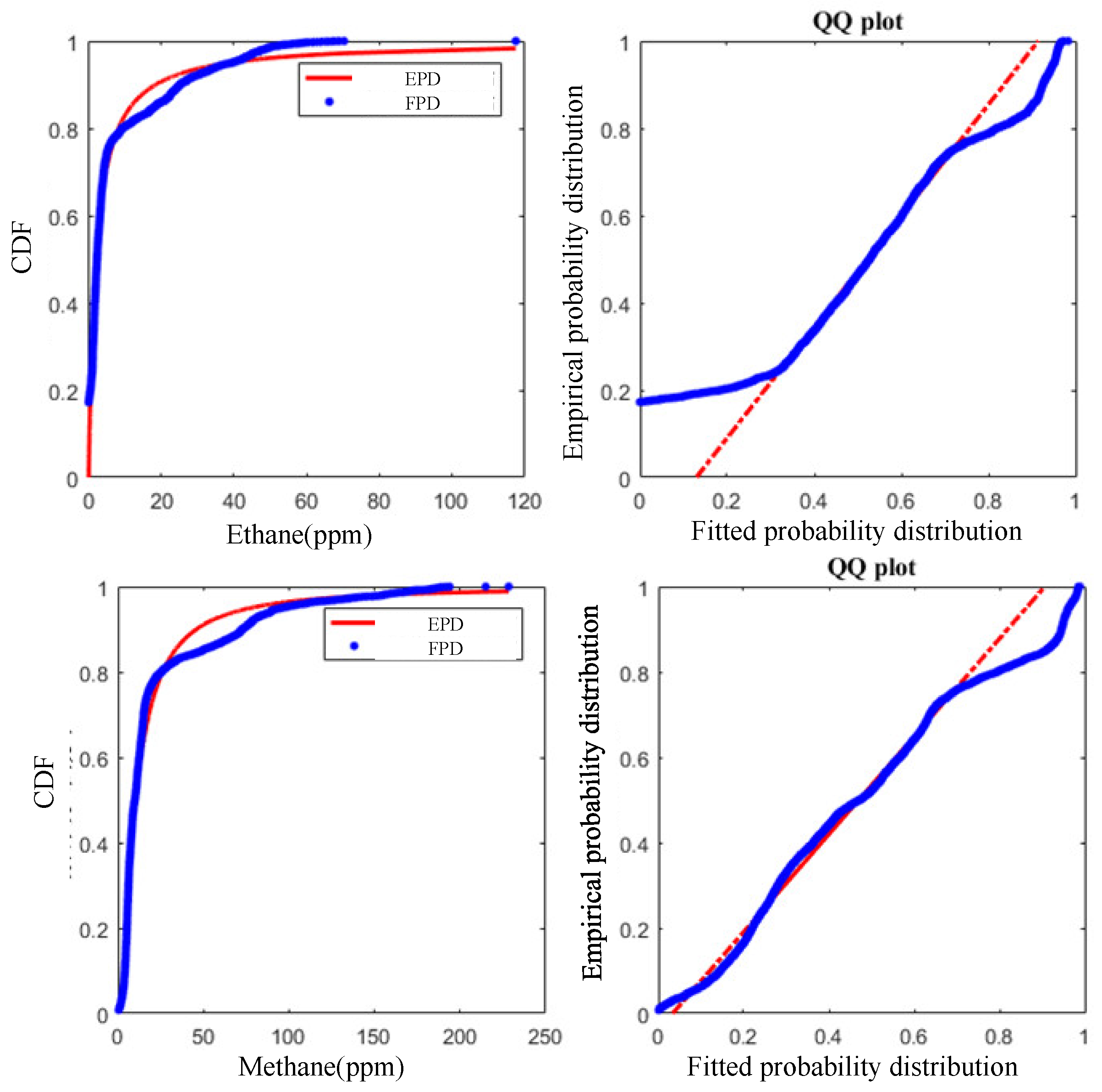
Finally, the copula function of methane and ethane with strong correlation are selected as the input variables. Then, the fitting of the marginal distribution type of the input variables is performed, the copula function type is selected, the copula function parameters are fitted in turn. The fitting distribution type of each marginal distribution variable is presented in the form of QQplot to visually verify whether a set of data comes from a certain distribution. The ordinate of the graph is the actual data in sorted order, which is called the empirical quantile, and the abscissa is the theoretical quantile of these data. The results can be seen in Figure 3.
The marginal distribution types of methane and ethane are the generalized extreme value distribution and generalized Pareto distribution, respectively. After obtaining the distribution types and parameters of methane and ethane, the cumulative distribution probability can be used as the input variable of the copula function, and the next step can be performed for copula function type fitting and selection.
4.3. Copula Function Selection and Fitting
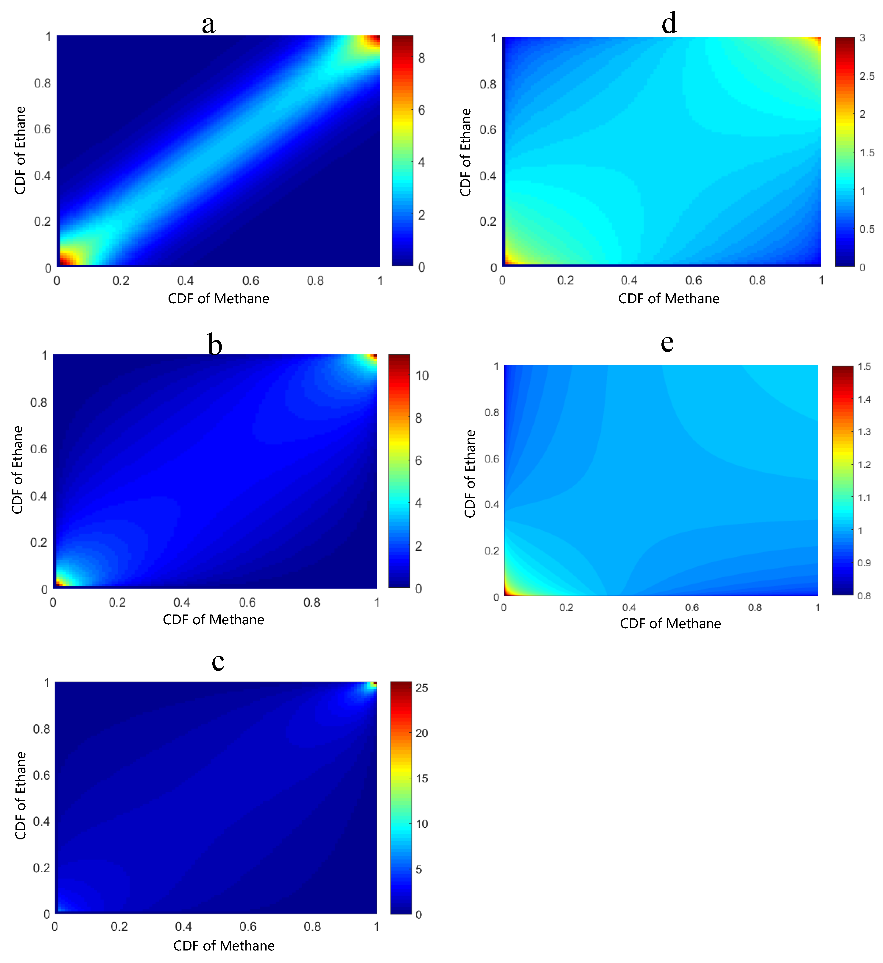
After determining the distribution type of the input variables, it is necessary to further determine the selection of the copula function and the fitting parameters through the maximum likelihood method. The probability density distribution of the copula function fitted by the dissolved gas in the oil is shown in Figure 4.
After fitting the parameters of the five copula functions, it is necessary to further evaluate the advantages and disadvantages of different copula functions for the fitting of dissolved gases in transformer oil. NSE and RMSE are the important indicators for evaluating the selection of copula functions. The value of each copula function is calculated separately, especially the root mean square error and Nash coefficient. The results are shown in Table 2.
The NSE index value corresponding to the Frank copula function is the largest, indicating that the Frank copula function can better describe the joint distribution of dissolved gases in transformer oil. The NMSE index value is the smallest, indicating that the results of the Frank copula function have the smallest error compared with the empirical distribution. Therefore, for the marginal distribution variable with copula joint distribution of methane and ethane, the Frank copula function is the best choice.
4.4. Transformer Status Diagnosis of Power Transformer
After obtaining the cumulative probability estimate of the variable and inputting it into the Frank copula function, the corresponding relationship between the cumulative distribution probability result of the copula function and the three states is shown in Figure 5.
It can be seen from the correspondence between the CDF results and the three states: even if the CDF results are not greater than 0.9, there are still concentrated fault data between 0.7 and 0.8. There will be errors in judging the transformer state simply by relying on the CDF range. It is necessary to propose a more rigorous judgment process.
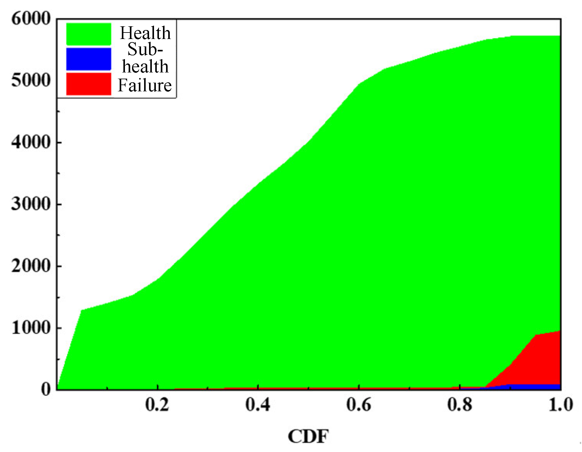
The concentrated distribution characteristics of the transformer fault states appear can be used as the basis for data state diagnosis, and the preliminary statistics of the three states are distributed as shown in Figure 6.
It can be seen from the CDF changes in the three states that when the CDF is greater than 0.6, the number of health data begins to decrease, and the failure data begins to appear when the CDF is greater than 0.7. When CDF = 0.9, the failure data increases sharply, and the sub-health data are mainly distributed in within the range of CDF > 0.9. According to the distribution characteristics of different state data, the preliminary diagnosis process is carried out. On the basis of KNN algorithm, the change of the probability of transformer state diagnosis as CDF increases is shown in Figure 7.
According to the results in Figure 7, when the CDF is less than 0.66, the probability of the health state data almost reaches 1. But when the CDF is greater than 0.66, the probability of the health data changes. The reason is that the CDF is concentrated between 0.7 and 0.8. Therefore, CDF = 0.66 can be used as the dividing line for the deterioration of the transformer state. When the CDF is greater than 0.8, the probability of the data being a fault state increases sharply. Thus, if the CDF result of the data is close to 0.8, the fluctuation of its gas concentration will cause the probability of the data diagnosis to be faulty and healthy to change sharply.
The DGA data in various literatures are different from each other; however, the field data of great value in this work prove the effectiveness of copula-based diagnosis technique.
5. Conclusions
It is difficult to establish the relationship of DGA data to the operation status of oil-immersed power transformers in a conventional manner, even with advanced machine-learning techniques without reliable prior knowledge. We proposed a copula function-based model to deal with actual DGA data to represent the working status in an efficient way in this article. Aiming at the application of copula function in the field of transformer condition diagnosis, this paper studied the variable selection of copula function, involving characteristic gas indicators, such as the hydrogen, methane, ethane, total hydrocarbons in dissolved gas in oil, and selecting the best fault characteristic gas as the input of the copula function, combined with actual field data and cases. The following conclusions were obtained:
- (1)
- Compared with other combinations of fault characteristic gases, the copula function CDF boundary whose marginal variable is hydrocarbon gas can separate the transformer healthy and faulty status, and the joint probability of the dissolved gas in oil is correlated with the transformer healthy or defective status.
- (2)
- When the CDF result of the dissolved gas in the oil in the copula function is close to 0.8, the fluctuation of its gas concentration leads to a sharp change in the probability that the data diagnosis results are defective or healthy.
- (3)
- Based on the correlation between the joint probability of dissolved gas in the oil and the transformer state (healthy or defective), the nearest neighbor algorithm can be used to evaluate the correlation between the data of the unknown state and the known state data in the copula function, and thus the unknown data state can be evaluated.
- (4)
- The binary copula function selected in this paper has a low degree of freedom and avoids deep network training. The copula function is used to separate the correlation structure between the marginal distribution and random variables, which simplifies the multivariate probability modeling process and is beneficial to field applications and implementation.
More work will be evaluated with regard to the increasing scale of DGA data of oil-immersed power transformers in the field in the near future.
Author Contributions
Conceptualization, X.Z. and R.W.; methodology, H.Z.; validation, B.L., J.J. and X.Z.; formal analysis, X.Z.; investigation, X.Z.; resources, X.Z.; data curation, B.L.; writing—original draft preparation, J.J.; writing—review and editing, X.Z.; visualization, J.J. All authors have read and agreed to the published version of the manuscript.
Funding
This research was funded by the State Grid Corporation Science and Technology Project, grant number 5200-202120090A-0-0-00.
Institutional Review Board Statement
Not applicable.
Informed Consent Statement
Not applicable.
Data Availability Statement
Not applicable.
Conflicts of Interest
The authors declare no conflict of interest.
Symbols and Acronyms
| AIC | Akaike information criterion |
| BIC | Bayesian information criterion |
| CDF | cumulative distribution probability |
| DGA | dissolved gas analysis |
| KMO | Kaiser–Meyer–Olkin |
| NSE | Nash coefficient |
| RMSE | root mean square error |
| THC | total hydrocarbons |
| k | the sample size |
| R | correlation matrix |
| Q | anti-image correlation matrix |
References
- Mahmoudi, N.; Samimi, M.H.; Mohseni, H. Experiences with transformer diagnosis by DGA: Case studies. IET Gener. Transm. Distrib. 2019, 13, 5431–5439. [Google Scholar] [CrossRef]
- Ghoneim, S.S.; Taha, I.B. A new approach of DGA interpretation technique for transformer fault diagnosis. Int. J. Electr. Power Energy Syst. 2016, 81, 265–274. [Google Scholar] [CrossRef]
- Jiang, J.; Chen, R.; Chen, M.; Wang, W.; Zhang, C. Dynamic Fault Prediction of Power Transformers Based on Hidden Markov Model of Dissolved Gases Analysis. IEEE Trans. Power Deliv. 2019, 34, 1393–1400. [Google Scholar] [CrossRef]
- Kim, S.-W.; Kim, S.-J.; Seo, H.-D.; Jung, J.-R.; Yang, H.-J.; Duval, M. New methods of DGA diagnosis using IEC TC 10 and related databases Part 1: Application of gas-ratio combinations. IEEE Trans. Dielectr. Electr. Insul. 2013, 20, 685–690. [Google Scholar] [CrossRef]
- Li, S.; Wu, G.; Gao, B.; Hao, C.; Xin, D.; Yin, X. Interpretation of DGA for transformer fault diagnosis with complementary SaE-ELM and arctangent transform. IEEE Trans. Dielectr. Electr. Insul. 2016, 23, 586–595. [Google Scholar] [CrossRef]
- Yang, D.; Qin, J.; Pang, Y.; Huang, T. A novel double-stacked autoencoder for power transformers DGA signals with an imbalanced data structure. IEEE Trans. Ind. Electron. 2021, 69, 1977–1987. [Google Scholar] [CrossRef]
- Malik, H.; Mishra, S. Application of Gene Expression Programming (GEP) in Power Transformers Fault Diagnosis Using DGA. IEEE Trans. Ind. Appl. 2016, 52, 4556–4565. [Google Scholar] [CrossRef]
- Taha, I.B.M.; Ibrahim, S.; Mansour, D.-E.A. Power Transformer Fault Diagnosis Based on DGA Using a Convolutional Neural Network with Noise in Measurements. IEEE Access 2021, 9, 111162–111170. [Google Scholar] [CrossRef]
- Chatterjee, K.; Dawn, S.; Jadoun, V.K.; Jarial, R. Novel prediction-reliability based graphical DGA technique using multi-layer perceptron network & gas ratio combination algorithm. IET Sci. Meas. Technol. 2019, 13, 836–842. [Google Scholar] [CrossRef]
- Ghoneim, S.S.M.; Taha, I.B.M.; Elkalashy, N.I. Integrated ANN-based proactive fault diagnostic scheme for power transformers using dissolved gas analysis. IEEE Trans. Dielectr. Electr. Insul. 2016, 23, 1838–1845. [Google Scholar] [CrossRef]
- Illias, H.A.; Chai, X.R. Hybrid modified evolutionary particle swarm optimisation-time varying acceleration coefficient-artificial neural network for power transformer fault diagnosis. Measurement 2016, 90, 94–102. [Google Scholar] [CrossRef]
- Liu, J.; Zheng, H.; Zhang, Y.; Li, X.; Fang, J.; Liu, Y.; Liao, C.; Li, Y.; Zhao, J. Dissolved Gases Forecasting Based on Wavelet Least Squares Support Vector Regression and Imperialist Competition Algorithm for Assessing Incipient Faults of Transformer Polymer Insulation. Polymers 2019, 11, 85. [Google Scholar] [CrossRef] [Green Version]
- Benmahamed, Y.; Kherif, O.; Teguar, M.; Boubakeur, A.; Ghoneim, S. Accuracy Improvement of Transformer Faults Diagnostic Based on DGA Data Using SVM-BA Classifier. Energies 2021, 14, 2970. [Google Scholar] [CrossRef]
- Huang, Y.-C.; Sun, H.-C. Dissolved gas analysis of mineral oil for power transformer fault diagnosis using fuzzy logic. IEEE Trans. Dielectr. Electr. Insul. 2013, 20, 974–981. [Google Scholar] [CrossRef]
- Bhalla, D.; Bansal, R.K.; Gupta, H.O. Integrating AI based DGA fault diagnosis using Dempster–Shafer Theory. Int. J. Electr. Power Energy Syst. 2013, 48, 31–38. [Google Scholar] [CrossRef]
- Islam, S.M.; Wu, T.; Ledwich, G. A novel fuzzy logic approach to transformer fault diagnosis. IEEE Trans. Dielectr. Electr. Insul. 2000, 7, 177–186. [Google Scholar] [CrossRef]
- Gouda, O.E.; El-Hoshy, S.H.; El-Tamaly, H.H. Proposed heptagon graph for DGA interpretation of oil transformers. IET Gener. Transm. Distrib. 2018, 12, 490–498. [Google Scholar] [CrossRef]
- Alghamdi, A.S.; Muhamad, N.A.; Suleiman, A.A. DGA Interpretation of Oil Filled Transformer Condition Diagnosis. Trans. Electr. Electron. Mater. 2012, 13, 229–232. [Google Scholar] [CrossRef] [Green Version]
- Illias, H.A.; Chai, X.R.; Abu Bakar, A.H.; Mokhlis, H. Transformer Incipient Fault Prediction Using Combined Artificial Neural Network and Various Particle Swarm Optimisation Techniques. PLoS ONE 2015, 10, e0129363. [Google Scholar] [CrossRef]
- Liu, Y.; Li, Y.; Ma, Y.; Jia, Q.; Su, Y. Development of a Bayesian-copula-based frequency analysis method for hydrological risk assessment—The Naryn River in Central Asia. J. Hydrol. 2020, 580, 124349. [Google Scholar] [CrossRef]
- Dehghani, E.; Ranjbar, S.; Atashafrooz, M.; Negarestani, H.; Mosavi, A.; Kovacs, L. Introducing Copula as a Novel Statistical Method in Psychological Analysis. Int. J. Environ. Res. Public Health 2021, 18, 7972. [Google Scholar] [CrossRef] [PubMed]
- Morteza, A.; Amirmazlaghani, M. A Novel Gaussian-Copula modeling for image despeckling in the shearlet do-main. Signal Processing 2022, 192, 108340. [Google Scholar] [CrossRef]
- Paul, D.; Goswami, A.K. Copula based bivariate modelling of DGA and breakdown voltage in high voltage transformers and reactors. IEEE Trans. Dielectr. Electr. Insul. 2019, 26, 1763–1770. [Google Scholar] [CrossRef]
Figure 1.
The process flow chart of dissolved gases in oil based on a copula function.

Figure 2.
Copula joint distribution of different variable combinations (Methane vs. Hydrogen, Methane vs. Ethane).
Figure 2.
Copula joint distribution of different variable combinations (Methane vs. Hydrogen, Methane vs. Ethane).

Figure 3.
Marginal distribution fitting results of methane and ethane.

Figure 4.
Copula function of the transformer oil color spectrum data fitting with methane and ethane. (a) Frank copula, (b) Gaussian copula, (c) Gumbel copula, (d) T copula, and (e) Clayton copula.
Figure 4.
Copula function of the transformer oil color spectrum data fitting with methane and ethane. (a) Frank copula, (b) Gaussian copula, (c) Gumbel copula, (d) T copula, and (e) Clayton copula.

Figure 5.
Corresponding relationship between CDF results of the copula functions and three states.

Figure 6.
The overall distribution of three state data under the change of CDF.

Figure 7.
Probability change of transformer state diagnosis under different CDF values.


Table 1.
Common factor loading of DGA.
| Dissolved Gases | Common Factor Loading #1 | Common Factor Loading #2 |
|---|---|---|
| H2 | 0.271 | 0.460 |
| CH4 | 0.916 | 0.301 |
| C2H6 | 0.993 | 0.085 |
| C2H4 | 0.774 | 0.602 |
| C2H2 | 0.088 | 0.746 |
| THC (total hydrocarbons) | 0.886 | 0.457 |
Table 2.
RMSE and NSE of different copula functions.
| Copula Function Type | RMSE | NSE | Parameters of Fitting |
|---|---|---|---|
| Gaussian | 1.1549 | 0.9767 | 0.8301 |
| T | 0.9455 | 0.9844 | 0.9001, 7.8203 |
| Frank | 0.7690 | 0.9897 | 15.9219 |
| Clayton | 1.8818 | 0.9382 | 1.3189 |
| Gumbel | 0.9886 | 0.9826 | 3.6969 |
Publisher’s Note: MDPI stays neutral with regard to jurisdictional claims in published maps and institutional affiliations. |
© 2022 by the authors. Licensee MDPI, Basel, Switzerland. This article is an open access article distributed under the terms and conditions of the Creative Commons Attribution (CC BY) license (https://creativecommons.org/licenses/by/4.0/).
Share and Cite
MDPI and ACS Style
Zhang, X.; Zhu, H.; Li, B.; Wu, R.; Jiang, J. Power Transformer Diagnosis Based on Dissolved Gases Analysis and Copula Function. Energies 2022, 15, 4192. https://0-doi-org.brum.beds.ac.uk/10.3390/en15124192
AMA Style
Zhang X, Zhu H, Li B, Wu R, Jiang J. Power Transformer Diagnosis Based on Dissolved Gases Analysis and Copula Function. Energies. 2022; 15(12):4192. https://0-doi-org.brum.beds.ac.uk/10.3390/en15124192
Chicago/Turabian StyleZhang, Xiaoqin, Hongbin Zhu, Bo Li, Ruihan Wu, and Jun Jiang. 2022. "Power Transformer Diagnosis Based on Dissolved Gases Analysis and Copula Function" Energies 15, no. 12: 4192. https://0-doi-org.brum.beds.ac.uk/10.3390/en15124192
Note that from the first issue of 2016, this journal uses article numbers instead of page numbers. See further details here.