Intelligent Tuned Hybrid Power Filter with Fuzzy-PI Control

Abstract

With the growing impact of power regulators, machines, and other power electronic devices on the quality of utility electric service, harmonics has recently emerged as a major research topic in the area of power quality and energy consumption. In this work, a fuzzy intelligent inductor–capacitor–inductor hybrid power filter is designed to reduce harmonics in the distribution line. The shunt active power filter and passive filter design and consideration have been improved. Since the nature of proportional integral control is only efficient with linear variations and the real condition of the distribution system is always varying nonlinearly, to create a minimum steady error, fuzzy-tuned proportional integral control is designed to intelligently consider the input changes and revise the decision rules using fuzzy reasoning. The content of the harmonic current with respect to the varying load is momentarily commutated. Thus, using Clarke’s transformation, the errors are summed with instantaneous power that is converted to a compensation current with the hysteresis band monitored pulse generator. The output current would turn off and on the IGBT inverter’s switches, supplying the current to reject the harmonics. The overall work was tested using MATLAB/SIMULINK^® and was effective in canceling harmonics.

1. Introduction

The increased use of power converters, machines, and other electronic devices in the distribution system has increased the content of harmonics. The effects of harmonics will create lagging power factors, mislead the remote control of the utility system, and could disconnect the customer loads from feeders. This problem will worsen during a load imbalance [1]. As a solution to this problem, passive filters were commonly used for harmonic suppression in earlier times. However, as these filters have a high switching resonance effect [2,3,4,5], the idea of using active filters has been given greater significance in filtering performance; still, because active filters also have maintenance issues, resonance effects, and less effect in large scale loads, the combined effects of active and passive power filters have gained prominence in recent times [2,4,6,7].

In this paper, the design improvement of a hybrid power filter is developed. The hybrid power filter is a combination of active and passive filters. The considerations and improvements in this work are also included for both of these. In the active filter design improvements in [8,9], the unbalanced voltage was considered as if it was created during filter action. In this work, however, the neutral voltage is considered both from the induced phase imbalance of the grid and the filtering circuit contribution. To determine the resonance frequency of HPF, the authors in [1,3,5,9,10,11,12] used the frequency response from the simulation of the transfer function peak gain and chose the frequency peak values. However, these values are the limits of the resonance frequency peaks under normal conditions.

During load variation, since the nonlinear parameter would also increase, the resonance would pass the limits. This work uses the limiting requirement in combination with a mathematically derived frequency peak formula to determine the system resonance frequency, and then, under these bounds, the value of the inductor, which is the major reason for the resonance frequency, is determined. Together with the filtering type, controllers also play an important role in filtering performance.

Controllers decide the value of filtering current and monitor the accurate injection of filtering current from the shunt active power filter (SAPF) or hybrid power filter (HPF) circuit. In this paper, to create efficient control for the unproportionable input variation, a fuzzy-tuned proportional integral (PI) controller is used. The rule-based fuzzy controller assists the PI controller in determining the new output by redirecting the outputs using the feedback controllers so that it can compare the variation of input with the previous inputs to determine the next precise value under the universe of discourse.

The reference computation mechanism can be based on the time or frequency domain. The frequency domain uses complex Fourier transforms or fast Fourier transforms for computing [1,13]. On the other hand, time-domain methods include Fryze–Buchholz–Dpenbrock (FBD), Genetic Algorithm (GA), instantaneous active-reactive power (PQ) theory method, and artificial neural network (ANN) methods [14]. This work uses the easiest time domain reference computing using PQ theory [1,15,16,17], which was originally proposed by Akagi in 1983 [18] and then improved for power reconditioning to calculate distorted voltage or current in power flow [10,18,19,20,21]. Once the reference current is generated, the active filtering procedure is guided by hysteresis bands. Fast and dynamic pulse generation will continue to turn on and off the converter so that the harmonic current is rejected.

The remaining part of this work is arranged as follows: Section 2 presents the proposed method, including the design of active, passive filter, and fuzzy control. In Section 3, the designed algorithm and flow chart are mentioned. Section 4 shows the simulation and comparison results, and Section 5 concludes the overall system output discoveries.

2. Proposed Idea

2.1. Research Contribution

As it is difficult to monitor the nonlinear load variation with the PI controller alone, fuzzy intelligent monitoring is added to support the PI controller. Fuzzy schemes are intelligent schemes that do not need an accurate mathematical model or linear input parameter. The input variation is intelligently monitored, and the control is redefined with input fuzzy rules to reconstruct the fuzzy set to output limits. Applying this proposed idea, this work addresses important issues in the design of inductor–capacitor–inductor hybrid power filter (LCL-HPF). These contributions include:

• A fuzzy-tuned PI controlled HPF is designed to increase the PI-controlling ability during load variation and system resonance.
• The active power filter design and voltage consideration are improved from [8], and [9]. In these articles, although the neutral voltage was considered, it should have been considered as an induced voltage to the filtering circuit. Thus, this article will consider the incoming phase voltage imbalance and the filter phase sequence as a result of this voltage action.
• In addition to the SAPF design criteria, this article also improves the design of the passive filter to be considered under all limiting conditions of resonance effect and the smoothing inductor element from the active filter part to be considered in passive circuit design. Thus, its values are considered during the maximum resonance finding.

2.2. LCL-HPF Filtering

The skeleton of the fuzzy-tuned LCL-HPF is shown in Figure 1. The basic circuit consists of the fuzzy controller, DC voltage source inverter (VSI), inductor, and shunt capacitor, which are coupled to the point of common coupling (PCC). The current from the active power filter side is represented by $i_{abcf}$, and the load current is designated by $I_{abcL}$. The current from reference is used to generate the compensation current, which is supplied to pulse modulation.

Parallel structured inverters and the SAPF filter coupling with the grid have similar characteristics, which are all affected by the condition of resonance and have remained the focus of research [6,22,23,24]. The mathematical and theoretical modeling and effects of parallel inverter resonance characteristics have been presented [6,22,23,24]. The discovery concluded that filtering inductance and impedance increase inverter resonance [6,25]. In this paper, the effect of resonance was the focus of design consideration. Thus, while the inverter side inductor (ISI) in LCL-HPF minimizes the ripples from the DC shunt capacitor, the grid side inductor (GSI) further suppresses the overall system variation and reduces the resonance effect. The capacitor eliminates higher order harmonics, as well as negative and zero sequence components during heavily loaded conditions.

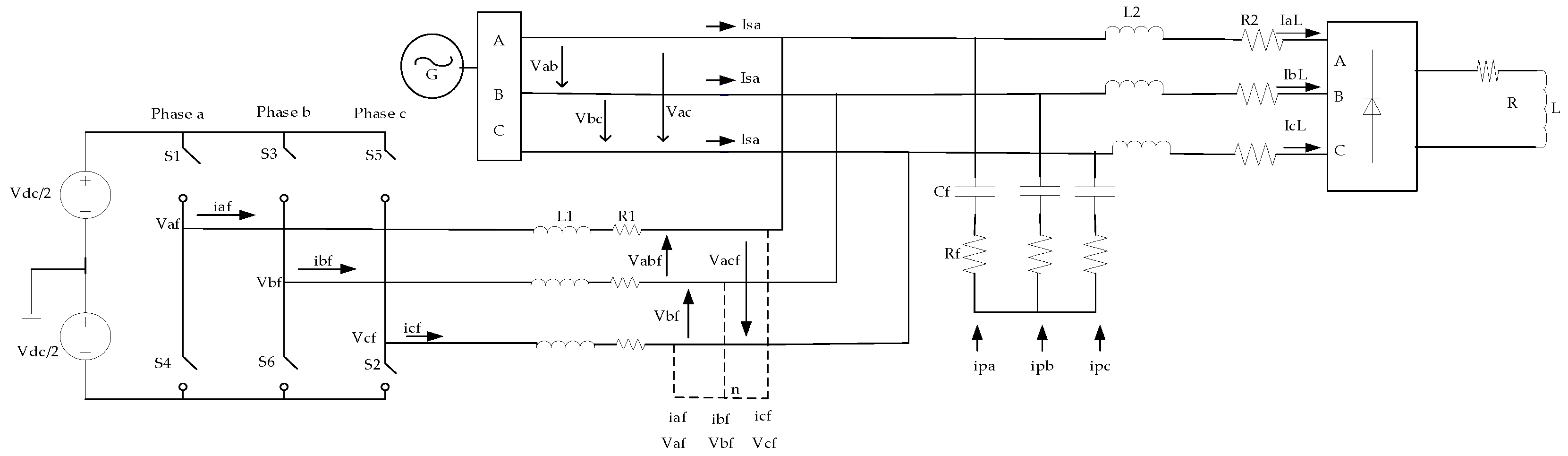
2.3. SAPF Design

In this section, the design of SAPF from [8,9] is improved. From Figure 2, the SAPF part applying Kirchhoff’s current law (KCL) and Kirchhoff’s voltage law (KVL), the phase to neutral voltage, can be given as:

$$V_{an}=i_{af}{R}_{af}+Ld\left(\frac{i_{af}}{dt}\right)+V_{fa}-V_n$$

(1)

where $V_n$ is the unbalanced voltage on the phases of active filter acquired from grid phase imbalance.

On the other hand, the unbalanced voltage can be computed from the zero-sequence voltage of the line in (2).

$$V_n=\frac{1}{3}\left(V_{af}+V_{bf}+V_{cf}\right)$$

(2)

The voltage injected from each phase for harmonic filtering is $V_{af}$, $V_{bf},$ and $V_{cf}$. Substituting for $V_n$ from (1) in (2),

$$-V_{an}+V_{fa}+i_{af}{R}_1+L_{1}d\left(\frac{i_{af}}{dt}\right)=\frac{1}{3}\left(V_{af}+V_{bf}+V_{cf}\right)$$

(3)

Expressing (3), in terms of the three-phase compensated voltage, (4) is discovered:

$$\left[V_{abcf}-V_n\right]=\frac{1}{3}\left[\begin{array}{ccc}-2& 1& 1\\ 1& -2& 1\\ 1& 1& -2\end{array}\right]\left[V_{abcf}\right]$$

(4)

where $\left[V_{abcf}\right]$=$\left[\begin{array}{c}{V}_{af}\\ V_{bf}\\ V_{cf}\end{array}\right]$, $\left[V_{abcf}-V_n\right]=\left[\begin{array}{c}{V}_{af}-V_n\\ V_{bf}-V_n\\ V_{cf}-V_n\end{array}\right]$.

The $\left[V_{abcf}-V_n\right]$ is the net applied voltages for filtering the current. Hence, $V_{abcf}-V_n$ is the new inverter line voltage. Re-expressing (4) the net filtering applied voltage with $V_{abcnf}$, it can be rewritten as:

$$\left[V_{abcnf}\right]=\frac{1}{3}\left[\begin{array}{ccc}-2& 1& 1\\ 1& -2& 1\\ 1& 1& -2\end{array}\right]\left[V_{abcf}\right]$$

(5)

where $\left[V_{abcnf}\right]=\left[\begin{array}{c}{V}_{af}-V_n\\ V_{bf}-V_n\\ V_{cf}-V_n\end{array}\right]$.

The voltage $V_{abcf}$ can be computed from the converter. Thus, the values are either 0 or $V_{DC}$ based on the sequence of switching. Further reducing this, (6) is obtained:

$$\left[V_{abcnf}\right]=\frac{1}{3}\left[J\right]\left[V_{abcf}\right]$$

(6)

where $\left[J\right]=\left[\begin{array}{ccc}-2& 1& 1\\ 1& -2& 1\\ 1& 1& -2\end{array}\right]$.

The current can be computed either from the inductor voltage in (9) or by applying KCL on the DC side of the inverter, the first half applied current can be estimated as presented as (7) and in three phases as (8):

$$\frac{L_{1}d{i}_{af}}{dt}=V_{af}-V_n+i_{af}{R}_1-V_{an}$$

(7)

Expressing in three phases, (8) is obtained:

$$\left[L_1\right]\left[\frac{d{i}_{abcf}}{dt}\right]=\left[\begin{array}{ccc}1& R_1& -1\end{array}\right]\left[\begin{array}{c}{V}_{abcf-V_n}\\ i_{abcf}\\ V_{abcn}\end{array}\right]$$

(8)

$$\frac{d{V}_{dc}}{dt}=\frac{1}{C_{dc}}\left\{\left(V_{anf}+2V_{bnf}\right)i_{af}+\left(2V_{anf}+V_{bnf}\right)i_{bf}\right\}$$

(9)

The converter switching would take place for the eight scenarios mentioned in

Table 1. Inverter switching operation and output voltage.

S	Inverter Switch Connection			Inverter Line Voltage			Inverter Phase Voltage
	${\mathit{V}}_{\mathit{a}\mathit{f}}$	${\mathit{V}}_{\mathit{b}\mathit{f}}$	${\mathit{V}}_{\mathit{c}\mathit{f}}$	${\mathit{V}}_{\mathit{a}\mathit{b}}\mathit{f}$	${\mathit{V}}_{\mathit{b}\mathit{c}\mathit{f}}$	${\mathit{V}}_{\mathit{c}\mathit{a}\mathit{f}}$	${\mathit{V}}_{\mathit{a}\mathit{n}\mathit{f}}$	${\mathit{V}}_{\mathit{b}\mathit{n}\mathit{f}}$	${\mathit{V}}_{\mathit{c}\mathit{n}\mathit{f}}$
1	+	+	+	0	0	0	0	0	0
2	−	+	+	$-V_{DC}$	0	$V_{DC}$	$-\frac{2}{3}{V}_{DC}$	$\frac{1}{3}{V}_{DC}$	$\frac{1}{3}{V}_{DC}$
3	+	−	+	$V_{DC}$	$-V_{DC}$	0	$\frac{1}{3}{V}_{DC}$	$-\frac{2}{3}{V}_{DC}$	$\frac{1}{3}{V}_{DC}$
4	+	+	−	0	$V_{DC}$	$-V_{DC}$	$\frac{1}{3}{V}_{DC}$	$\frac{1}{3}{V}_{DC}$	$-\frac{2}{3}{V}_{DC}$
5	−	−	+	0	$-V_{DC}$	$V_{DC}$	$-\frac{1}{3}{V}_{DC}$	$-\frac{1}{3}{V}_{DC}$	$\frac{2}{3}{V}_{DC}$
6	+	−	−	$V_{DC}$	0	$-V_{DC}$	$\frac{2}{3}{V}_{DC}$	$-\frac{1}{3}{V}_{DC}$	$-\frac{1}{3}{V}_{DC}$
7	−	+	−	$-V_{DC}$	$V_{DC}$	0	$-\frac{1}{3}{V}_{DC}$	$\frac{2}{3}{V}_{DC}$	$-\frac{1}{3}{V}_{DC}$
8	−	−	−	0	0	0	0	0	0

with the following conditions:

$$\left[V_{abcf}\right]=\{\begin{array}{c}1, if S_{k}is ON and S_{k+3} is OFF\\ 0, if S_{k}is ON and S_{k+3} is ON\end{array}$$

(10)

2.4. LCL-Passive Filter Modeling

The maximum power factor variation on the grid should not exceed 5% during reactive power compensation. Using this basic concept, the required compensation capacitor can be designed using the base impedance and grid angular frequency ($\omega$).

$$Z_b=\frac{V_s^2}{P_n}$$

(11)

where $V_s$ is the line to line voltage, $Z_b$ is the base impedance, and $P_n$, is the line power.

$$C_b=\frac{1}{\omega Z_b}$$

(12)

where $C_b$ is the base capacitance,$C_f$ is the required passive filtering capacitor, and $\omega$ is the grid angular frequency.

$$C_f=0.05C_b$$

(13)

The maximum ripple current ($∆I_{Lmax}$) at the output of a DC/AC inverter is given by:

$$∆I_{Lmax}=\frac{2V_{DC}}{3L_{max}}\left(1-m\right)m{T}_{sw}$$

(14)

In (14), the maximum peak-to-peak ripple current occurs at m = 0.5. Thus, the required series inductor from the inverter side ($L_{max}$) is computed as:

$$L_{max}=\frac{2V_{DC}}{6f_{sw}∆I_{Lmax}}$$

(15)

For 10% ripple of rated current (I_max), the design parameter is given by:

$$∆I_{Lmax}=0.1I_{max}$$

(16)

The maximum current is given as:

$$I_{max}=\frac{P_n\sqrt{2}}{3V_{ph}}$$

(17)

where $V_{ph}=\frac{V_s}{\sqrt{3}}$.

The damping resistance can be calculated as:

$$R_f=\frac{1}{{\omega }_{res}{C}_f}$$

(18)

The design procedures mentioned in (11)–(18) are from [8,9,11,26,27]:

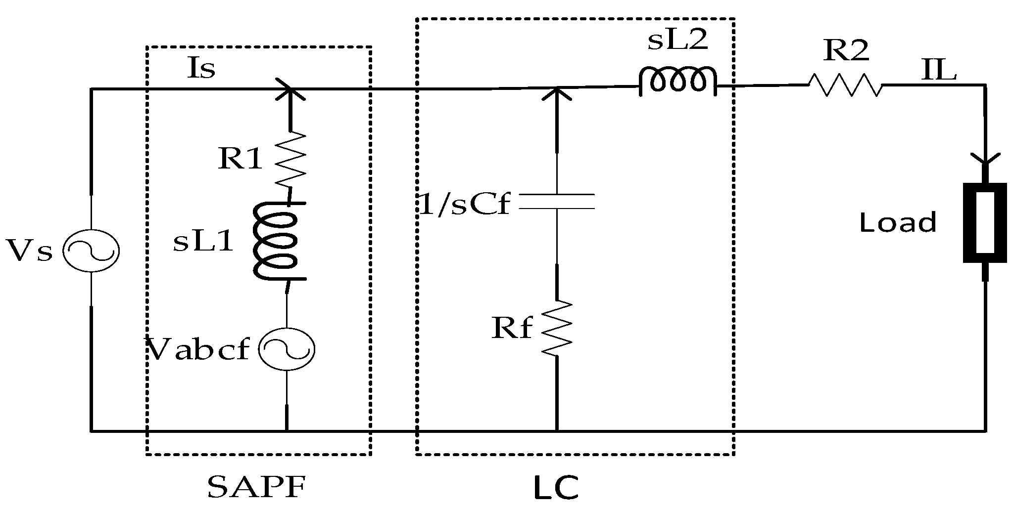
The consideration of resonance and its effect in filter design, where passive circuits are included, is fundamental. In order to determine these values, the inductor and capacitor must be considered alongside the effect of grid voltage and the resonance limit of the transfer function. The RLC circuit transfer function of Figure 2 can be given as (19):

$$Y\left(s\right)=\frac{i_{in}}{V_S-V_{abcf}}=\frac{1}{Z_{th}+\left(R_2+s{L}_2\right)}$$

(19)

$$Z_{th}=\frac{s^2{R}_f{L}_1{C}_f+s\left(R_1{R}_f{C}_f+L_1\right)+R_1}{s{C}_f}$$

(20)

The transfer function is

$$Y\left(s\right)=\frac{s{C}_f}{s^2\left(R_f{L}_1{C}_f+C_f{L}_2\right)+s\left(R_1{R}_f{C}_f+L_1+R_2{C}_f\right)+R_1}$$

(21)

In various articles [1,3,5,9,10,11,12], the resonance frequency was found by using the poles of Y(s) (i.e., the condition where $Y\left(s\right)\to \infty$) and then applying the quadratic formula for second order and higher transfer functions.

In this article, the maximum resonance is considered to determine the resonance frequency limit of the circuit. The maximum resonance can be found from the first derivative of the transfer function i.e., (dY(s))/ds = 0. As a result, (21) is reduced to (25):

$$\frac{dY\left(s\right)}{ds}=\frac{\begin{array}{c}{C}_f\left[s^2\left(R_f{L}_1{C}_f+C_f{L}_2\right)+s\left(R_1{R}_f{C}_f+L_1+R_2{C}_f\right)+R_1\right]\\ -2s\left[\left(R_f{L}_1{C}_f+C_f{L}_2\right)+\left(R_1{R}_f{C}_f+L_1+R_2{C}_f\right)\right]s{C}_f\end{array}}{{\left(s^2\left(R_f{L}_1{C}_f+C_f{L}_2\right)+s\left(R_1{R}_f{C}_f+L_1+R_2{C}_f\right)+R_1\right)}^2}=0$$

(22)

$$-s^2\left(R_f{L}_1{C}_f+C_f{L}_2\right)+R_1=0$$

(23)

$${\omega }_{res}^2=\frac{R_1}{C_f\left(R_f{L}_1+L_2\right)}$$

(24)

$$f_{res}=\frac{1}{2\pi \sqrt{\raisebox{1ex}{$C_f$}\!\left/ \!\raisebox{-1ex}{$R_1$}\right.\left(R_f{L}_1+L_2\right)}}$$

(25)

From the boundary of the frequencies, it is possible to find the threshold of the inductor and impedance values. In passive filter design, the limiting requirements of (26) are given [11,26,27]:

$$10f<f_{res}<0.5f_{sw}$$

(26)

Using the limiting requirements of (26), substituting the value of resonance frequency obtained from the transfer function of the LCL-HPF circuit given in Figure 2 is reduced to (27) and (28).

$$100f^2<{\left(\frac{1}{2\pi \sqrt{\raisebox{1ex}{$C_f$}\!\left/ \!\raisebox{-1ex}{$R_1$}\right.\left(R_f{L}_1+L_2\right)}}\right)}^2<0.25f_{sw}^2$$

(27)

$$\frac{R_1}{{\left(\pi f_{sw}\right)}^2{C}_f}<R_f{L}_1+L_2<\frac{R_1}{{\left(20\pi f\right)}^2{C}_f}$$

(28)

Since the inverter side inductor is the higher, considering the upper frequency limit:

$$R_f{L}_1+L_2=\frac{R_1}{{\left(20\pi f\right)}^2{C}_f}$$

(29)

The actual value of the required inductor on the line from the inverter side was $L_{max}$. However, $L_1$ is connected parallel to the line. Since the actual $L_1$ should be obtained first in (29), expressing $L_2$ from the transfer function in terms of $L_1$, the approximate value can be obtained from parallel combinations.

$$L_2=\frac{1}{R_f}\left[\frac{R_1}{{\left(20\pi f\right)}^2{C}_f}-R_f{L}_1\right]$$

(30)

Parallel combinations would have less than the smallest value. Considering the inductor value in (15) the inverter inductor can be solved from (32).

$$\frac{L_2{L}_{max}}{L_2+L_{max}}\approx L_2$$

(31)

$$\frac{\left(\frac{1}{R_f}\left[\frac{R_1}{{\left(20\pi f\right)}^2{C}_f}-R_f{L}_1\right]\right)\left(\frac{V_{dc}}{6f_{sw}∆I_{max}-V_{dc}}\right)}{\frac{1}{R_f}\left[\frac{R_1}{{\left(20\pi f\right)}^2{C}_f}-R_f{L}_1\right]+\frac{V_{dc}}{6f_{sw}∆I_{max}-V_{dc}}}$$

$$R_f{L}_1^2+L_1\left(L_T{R}_f-x+L_{max}\right)-x{L}_{max}=0$$

$$L_1=\frac{-\left(L_{max}{R}_f-x+L_{max}\right)+\sqrt{{\left(L_{max}{R}_f-x+L_T\right)}^2-4\left(x{R}_f{L}_{max}\right)}}{2R_f}$$

(32)

where $x=\frac{R_1}{{\left(20\pi f\right)}^2{C}_f}$.

2.5. Fuzzy Controller Design

Fuzzy is an intelligent scheme which is composed of fuzzy rules, fuzzification, fuzzy inference, and premises. It is capable of mimicking and simulating human learning behavior [12]. As fuzzy intelligence does not require precise mathematical modeling, it can solve a variety of computable models in the system.

The distribution system would never be assumed to stay stable at a certain level since the customers would come in and out of the system at unpredictable times. This means the fuzzy membership values (membership degrees) would also change values in the range of 0 to 1. The non-fuzzy controlling values are assigned with linguistic terms to these membership values with a defined range of discourse, the input increase or decrease is regularly measured together with the feedback input. In both cases, the new fuzzy rules would generate adjustments either to increase or decrease the membership values. For this reason, the triangular membership function was chosen in this research.

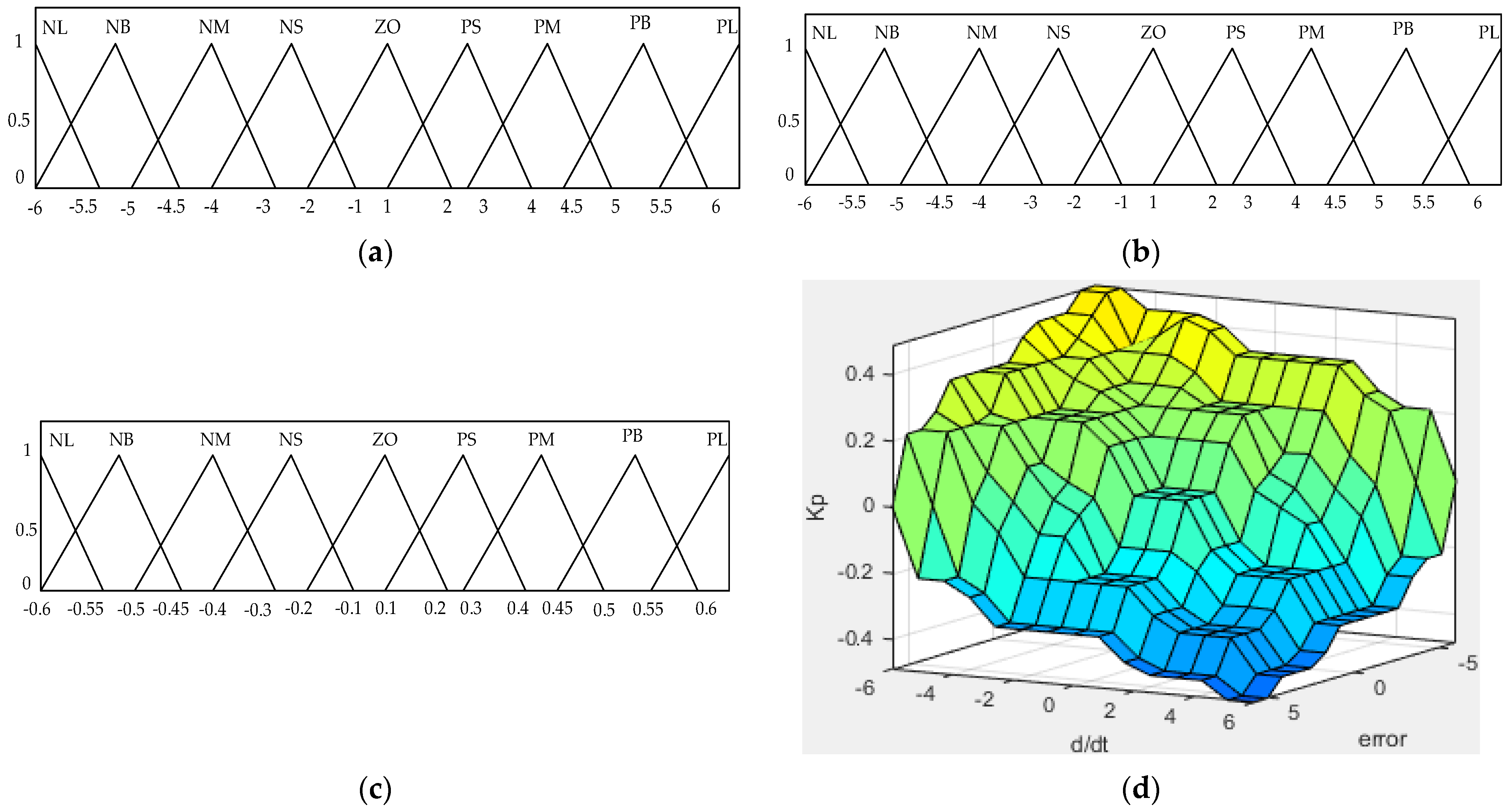
A fuzzy controller requires a fuzzy rule to adjust the control based on the conditions in order to keep the capacitor and reference voltage difference constant. In this work, there are 81 Mamdani rules to control the input–output dynamics. In general, this design has two basic inputs in its constrained domain, called the universe of discourse. The first is error with a universe of discourse [−6, 6], as shown in Figure 3a, and the second is the rate of change of variation error in its universe of discourse [−6, 6] as shown in Figure 3b.

The output of a fuzzy controller is computed by exchanging the rule base membership functions with the universe of discourse [−0.6, 0.6] as shown in Figure 3c’s fuzzy membership function. The notations mentioned in

Table 2. Fuzzy control rules.

$\mathbf{∆}\mathit{K}\mathit{P}$		e
		NL	NB	NM	NS	ZO	PS	PM	PB	PL
$\frac{d}{dt}$	NL	PL	PL	PB	PB	PM	PM	PS	PS	ZO
	NB	PL	PL	PB	PM	PM	PS	PS	ZO	NS
	NM	PB	PB	PM	PM	PS	PS	ZO	NS	NS
	NS	PB	PB	PM	PS	PS	ZO	NS	NM	NM
	ZO	PM	PM	PS	PS	ZO	NS	NS	NM	NM
	PS	PM	PM	PS	ZO	NS	NM	NM	NB	NB
	PM	PS	PS	ZO	NS	NS	NM	NM	NB	NB
	PB	PS	ZO	NS	NM	NM	NB	NB	NL	NL
	PL	ZO	NS	NS	NM	NM	NB	NB	NL	NL

are divided into positive and negative membership functions. The negative and positive domains, where {NL, NB, NM, NS, ZO} represent negative very large, negative large, negative medium, negative small, and zero, respectively; and {PL, PB, PM, PS} represent positive very large, positive large, positive medium, and positive small, respectively.

The 3D plot of the output control can be seen from Figure 3d. From the figure, it can be seen that errors are optimum when the system difference is near to zero, which means the designed system will exchange intelligently the input rules that can best fit the minimum steady output error by reconfiguring the fuzzy rules.

2.6. Controller Robustness and Stability

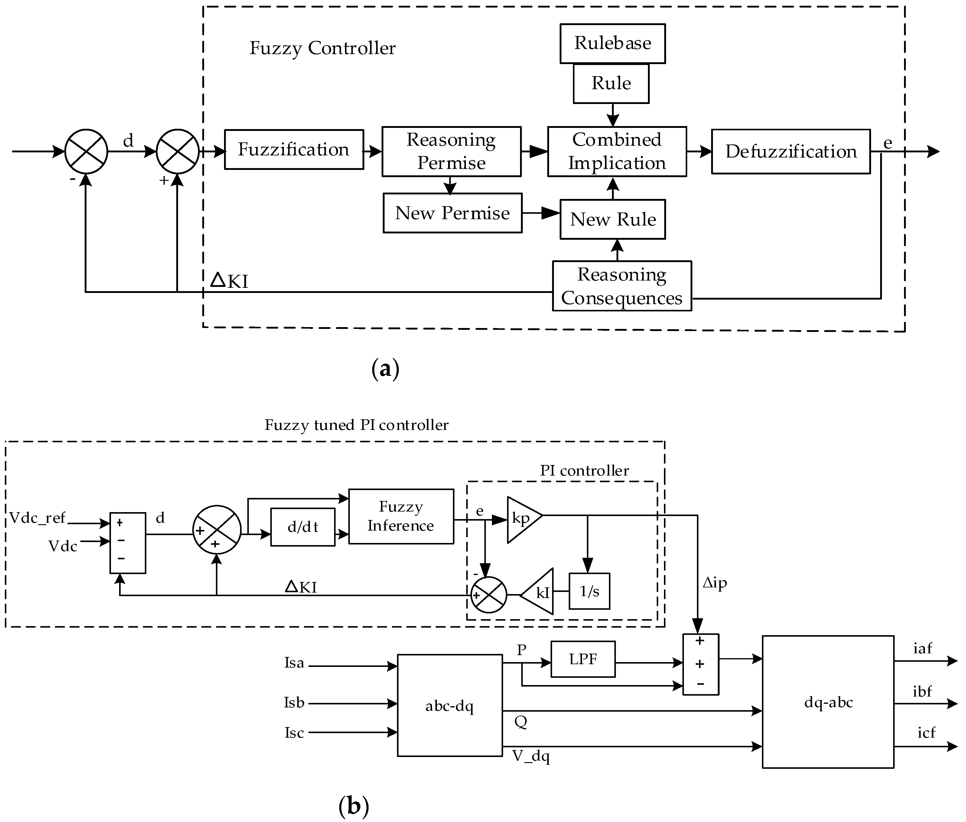
The control diagram in Figure 4a,b shows that compensation current is maintained by controlling the input voltages from the DC capacitor, which is used as the input of the hysteresis band guided modulator. The error from the differences in the capacitor voltage and the reference voltage needs to be steady, and the feedback controllers consider the differences in output errors with the foregoing errors. Then, the reasoning premises are modified according to the new changes in errors. Following the forward implication, the defuzzied output variation is measured with the to-go next outputs using the feedback as a result of optimal reasoning, and the rules are updated to discover the minimum output.

The robustness of fuzzy reasoning with conventional controllers was studied with a PID controller in [28]. The authors presented inference-based reasoning both in conventional and optimal fuzzy reasoning, where the fuzzy reasoning method (FRM) was aimed at achieving optimal feedback control. This filtering circuit also has two feedback controls for optimization, which act on input–output variation as a consequence of load variation and the resonance effect of nonlinear loads. Considering the feedback control from Figure 4, the output gains can be determined using the following three conditions:

• When the defuzzied output values reaches the upper limits in the universe of discourse, the output will consequently increase, and the feedback responds using the subtracting feedback controller.

$$G1\left(s\right) =\frac{e{k}_p{k}_I}{ s+k_P{k}_I\left(1-e\right)}$$

(33)

2.

When the defuzzied output reaches the lower limits of the universe of discourse, the feedback values is added to the inputs.

$$G2\left(s\right)=\frac{e{k}_p{k}_I}{s+k_P{k}_I\left(1+e\right)}$$

(34)

3.

When the system condition is stable and the values are at the mid values of the output universe of discourse, the feedback gain is as follows:

$$G3\left(s\right)=\frac{de{k}_p{k}_I}{s+k_p{k}_I\left(1-e\left(1-d\right)\right)}$$

(35)

According to Equations (33)–(35), the feedback value will stabilize the output by supplying or subtracting from the inputs, and the fuzzy rules are updated using this input–output consequence of reasoning.

2.7. PQ Compensation Method

The time and frequency domains are the general categories used for finding the reference current [29]. This work employs PQ theory, which is accomplished by transforming $abc$ reference coordinates to α-β coordinates, a process known as Clarke’s transformation [29].

$$\begin{array}{c}{V}_{\alpha }\\ V_{\beta }\end{array}=\sqrt{\frac{2}{3}}\left[\begin{array}{ccc}1& -\raisebox{1ex}{$1$}\!\left/ \!\raisebox{-1ex}{$2$}\right.& -\raisebox{1ex}{$1$}\!\left/ \!\raisebox{-1ex}{$2$}\right.\\ 0& \raisebox{1ex}{$\sqrt{3}$}\!\left/ \!\raisebox{-1ex}{$2$}\right.& \raisebox{1ex}{$-\sqrt{3}$}\!\left/ \!\raisebox{-1ex}{$2$}\right.\end{array}\right]\left[\begin{array}{c}{V}_{sa}\\ V_{sb}\\ V_{sc}\end{array}\right]$$

(36)

$$\begin{array}{c}{i}_{\alpha }\\ i_{\beta }\end{array}=\sqrt{\frac{2}{3}}\left[\begin{array}{ccc}1& -\raisebox{1ex}{$1$}\!\left/ \!\raisebox{-1ex}{$2$}\right.& -\raisebox{1ex}{$1$}\!\left/ \!\raisebox{-1ex}{$2$}\right.\\ 0& \raisebox{1ex}{$\sqrt{3}$}\!\left/ \!\raisebox{-1ex}{$2$}\right.& \raisebox{1ex}{$-\sqrt{3}$}\!\left/ \!\raisebox{-1ex}{$2$}\right.\end{array}\right]\left[\begin{array}{c}{I}_{sa}\\ I_{sb}\\ I_{sc}\end{array}\right]$$

(37)

where $V_{sa}, V_{sb}, V_{sc}$ and, $I_{sa}, I_{sb}, I_{sc}$ refer, respectively, to the three-phase voltage and currents in the $abc$ coordinates. $V_{o, } V_{\alpha }, V_{\beta }$ and $i\alpha , i\beta$ represent the three-phase voltage and currents at α-β coordinates, respectively.

The active ($P$) and reactive ($Q$) power is obtained instantaneously as [29], (38):

$$\left[\begin{array}{c}P\\ Q\end{array}\right]=\left[\begin{array}{cc}{V}_{\alpha }& V_{\beta }\\ V_{\beta }& -V_{\alpha }\end{array}\right]\left[\begin{array}{c}{i}_{\alpha }\\ i_{\beta }\end{array}\right]$$

(38)

The average power, circulating current and voltage from shunt capacitor ($I+∆I and V+∆V$) are consumed by filtering capacitor $C_f$. The $P$ and $Q$ seen in Figure 4b can be divided to oscillatory and average terms $P={}_P{}^{~}l+pl$ and $Q={}_q{}^{~}l+Ql$. The average power part consists of first harmonic positive sequence, i.e., $i{l}_{nh}^{\pm }+i{l}_{nh}^{-}$ after the low pass filter. Hence, to keep the filtering stable, while the primary oscillatory power components, compensated by the SAPF, the remaining and average power components are eliminated by the LCL filter where $pc={}_{-P}{}^{~}l$ and $qc={}_{-q}{}^{~}l.$ The compensation current is obtained by inverting the matrix [29].

$$\left[\begin{array}{c}i{C}_{\alpha }\\ i{C}_{\beta }\end{array}\right]=\frac{1}{V_{\alpha }^2+V_{\beta }^2}\left[\begin{array}{cc}{V}_{\alpha }& V_{\beta }\\ V_{\beta }& -V_{\alpha }\end{array}\right]\left[\begin{array}{c}pc\\ qc\end{array}\right]$$

(39)

$$\left[\begin{array}{c}{i}_{af}\\ i_{bf}\\ i_{cf}\end{array}\right]=\sqrt{\frac{2}{3}}{\left[\begin{array}{ccc}1& -\raisebox{1ex}{$1$}\!\left/ \!\raisebox{-1ex}{$2$}\right.& \raisebox{1ex}{$-1$}\!\left/ \!\raisebox{-1ex}{$2$}\right.\\ 0& \raisebox{1ex}{$\sqrt{3}$}\!\left/ \!\raisebox{-1ex}{$2$}\right.& -\raisebox{1ex}{$\sqrt{3}$}\!\left/ \!\raisebox{-1ex}{$2$}\right.\end{array}\right]}^T\left[\begin{array}{c}i{C}_{\alpha }\\ i{C}_{\beta }\end{array}\right]$$

(40)

2.8. Current Injection Technique

The hysteresis-banded (HB) pulse generator was chosen due to its effectiveness for high switching response, accuracy, and unconditioned stability [25]. In this method, the current is projected from the fuzzy-tuned PI controlled current source and is injected to VSI at a preplanned width of the band (HB). The maximum errors on the band will turn OFF the VSI switches, and the minimum will turn it ON. This process will let the DC shunt capacitor current be injected to cancel the harmonic currents.

3. Working Algorithm

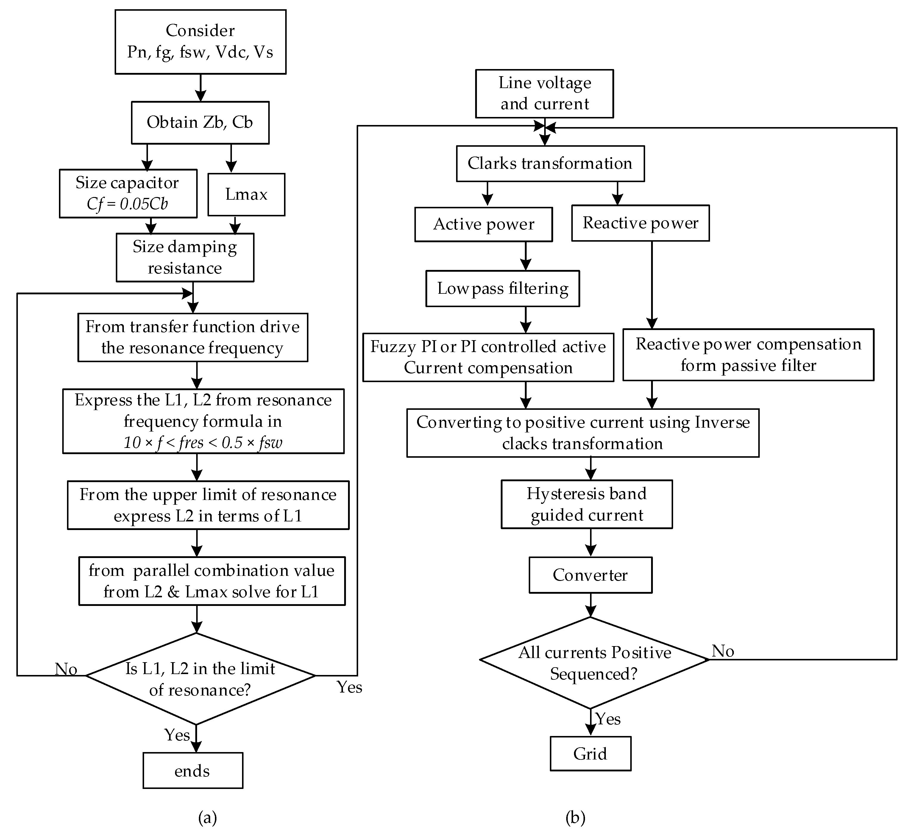
The LCL-HPF algorithmic presented in Figure 5 can be described as follows:

• Compute the passive and active circuit using Figure 5a.
• The three-phase non-linear loaded line is connected to the fuzzy-tuned HPF filtering.
• Using Clark’s Transformation, the active and reactive current component and voltage are decomposed.
• The active power component would pass through a low pass filter, and then the active component of power is subtracted from the errors of the fuzzy-tuned PI controller injected power.
• The reactive power component was already compensated on the line from the inductor–capacitor–inductor (LCL) circuit; thus, the SAPF would not be expected to generate reactive power.
• Both the active and reactive components are converted to three phase current and voltage components using the inverse Clarkes transformation. This time, the line current is converted to a positive sequence current as required by the grid.
• The converter is guided by the hysteresis band-controlled pulse modulator based on the switching sequences and current presented in (9). Along with the voltage in Table 1, it injects the filtering current on the grid.
• The ripples from the active power filter is filtered by the seriously connected inductor.
• Unbalanced, nonpositive sequenced current and the average power are consumed by the LC filters, and the remainder is eliminated after several cycles in the LCL and SAPF filtering circuits.

4. Results and Discussion

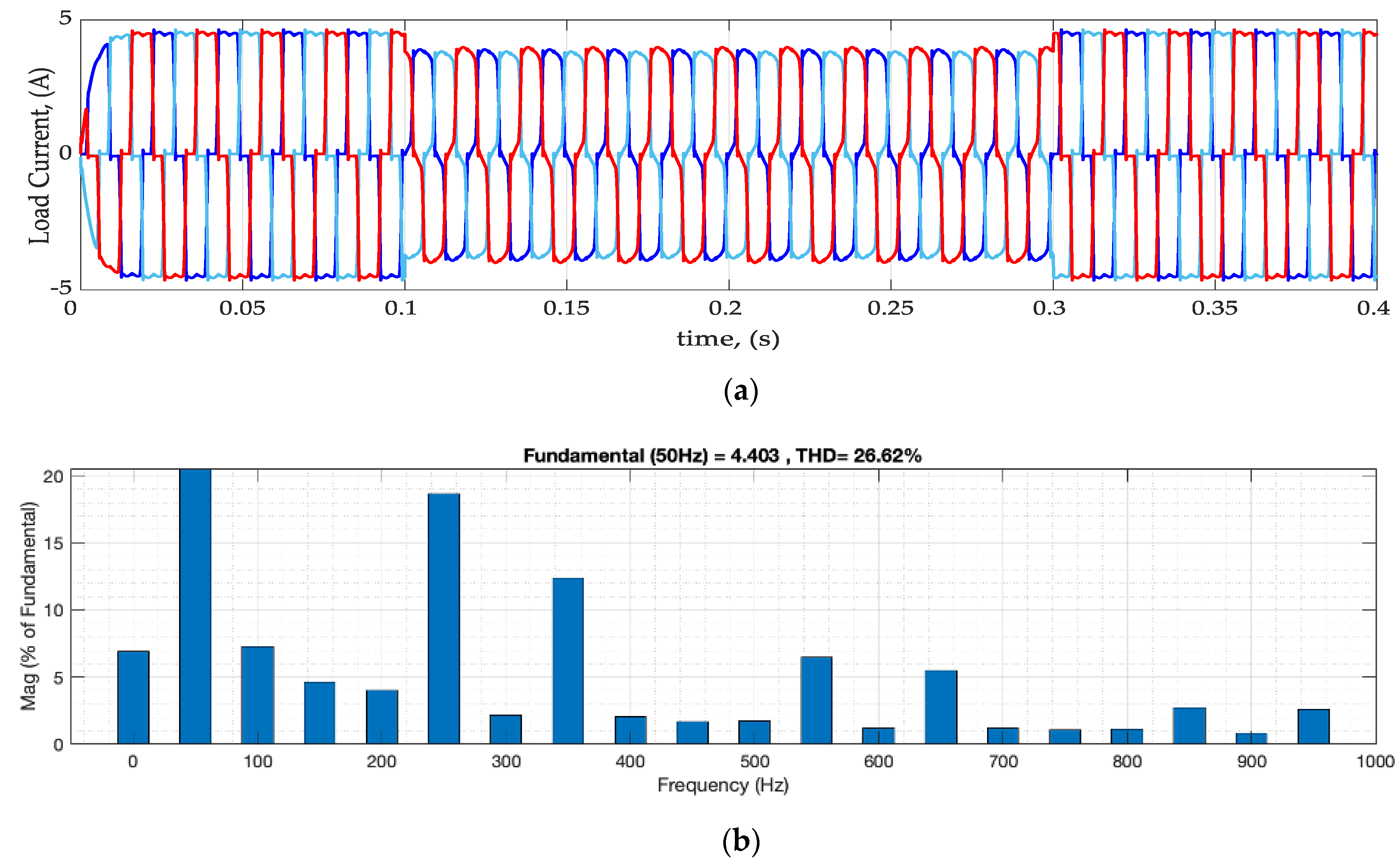
The simulation inputs for this work are presented in

Table 3. Designed HPF parameter values and considered test loads.

Item	Value
Source/Grid	10 kW, 208 Vs, 50 Hz
$L_1$	20 mH
$L_2$	0.254 mH
$f, f_{res}, f_{sw}$	50$\mathrm{kHz}$, 7000$\mathrm{kHz}$, 15,000 $\mathrm{kHz}$
$C_f$	36.8$\mathsf{\mu }\mathrm{F}$
$R_1, R_2, R_f, R_2$	$1\mathsf{\Omega }, 1.5 \mathsf{\Omega }, 0.1, 1 \mathsf{\Omega }$
$C_f$ of passive filter = Dc-link capacitor	36.8$\mathsf{\mu }\mathrm{F}$
Load	60 Ω, 200 mH
Vdc	450 V
Unbalanced resistive Load phase ABC	100 w, 90 w, 110 w
Unbalanced Inductive reactive Load phase ABC	10, 9, 11 Var
Unbalanced Inductive reactive Load phase ABC	10, 9, 11 Var
Proportional gain (Kp)	2/5
Integral gain (Ki)	4

. It can be seen that the load is composed of resistor, capacitor, and inductor. As mentioned previously, the entire design is implemented using MATLAB Simulink^®. The load current was no longer sinusoidal, as shown in Figure 6a, and the total harmonic distortion (THD) of the system was also 26.6, as shown in Figure 6b. If not properly managed, the collective effect of harmonics would hugely disturb the grid, especially on the operation of remote protection control and utility customers.

To address this harmonic issue, the designed fuzzy-tuned PI controlled HPF is presented in comparison with the PI controlled HPF. In both conditions, the parameters of load, filtering inputs, and harmonic computation time are fixed the same as presented in Table 3. To observe the control responses, the load is forced to change by adding and removing the unbalanced three-phase nonlinear load as shown in Figure 6a. The simulation procedures and results are discussed in each section.

4.1. Filtering Current Injection and DC Shunt Capacitor Switching

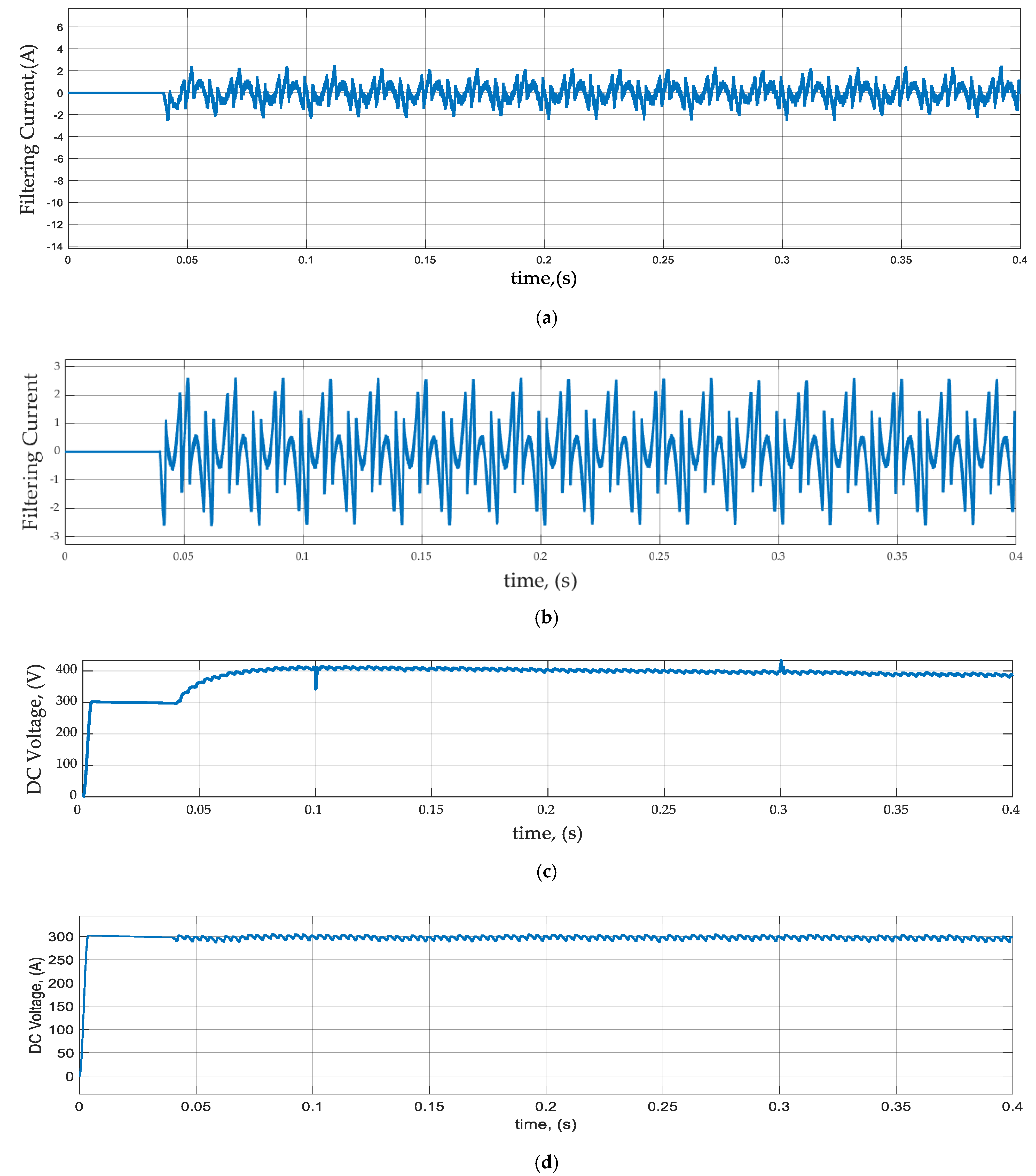
Using the values from Table 3, the performance with filtering current injection and shunt capacitor switching waveforms from the MATLAB Simulink^® test are shown in Figure 7a–d, respectively. From the output of the filtering current in Figure 7a, the wave of the injected current by the PI controller has a relatively thick and lower amplitude compared to the amplitudes of the fuzzy-tuned PI controller output seen in Figure 7b. This shows that the fuzzy-tuned PI controller has better reached the harmonic peak current during rejection where the injected current is created by the response of the controller that is used to guide the reference current. The better controller has a small steady error and can reject harmonics better as seen on the fuzzy-tuned PI controller.

On the other hand, Figure 7c,d shows the performance of the DC voltage. From Figure 7c, it can be seen that the PI controlled HPF’s DC voltage starts late, and its performance is influenced by load variation. The DC voltage wave produces spikes when the load changes, and while the MATLAB test did this by changing the load only two times, these changes would happen frequently on the real distribution line. Thus, the loads would receive frequent spiking waves, which could damage the customers’ equipment. From Figure 7d, however, the fuzzy-tuned PI controller wave becomes straight and achieves stability. This indicates that the feedback has learnt from the consequences of reasoning and helped the fuzzy premises redefine the decisions in every load variation immediately.

4.2. Grid Current and Total Harmonic Distortion

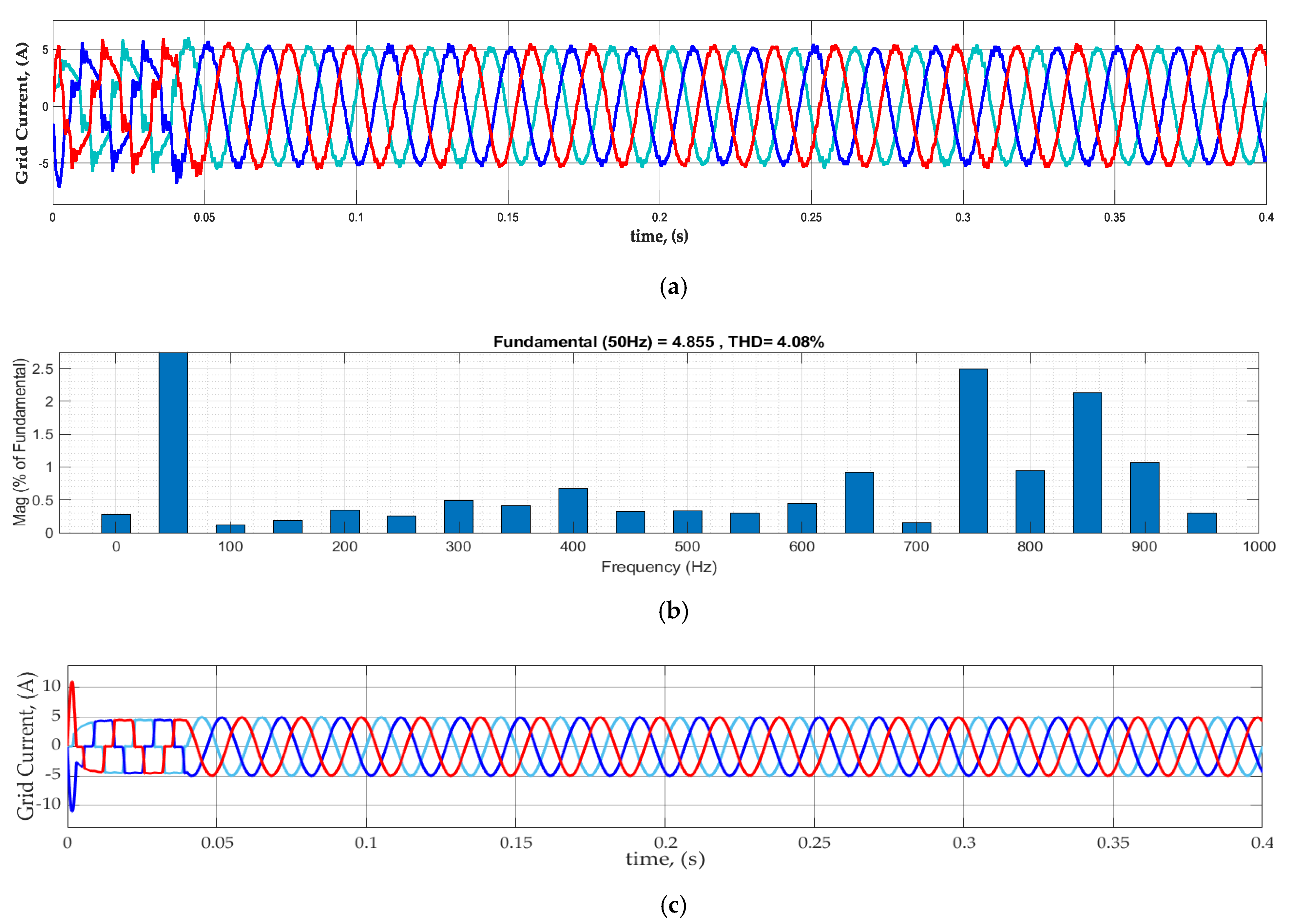
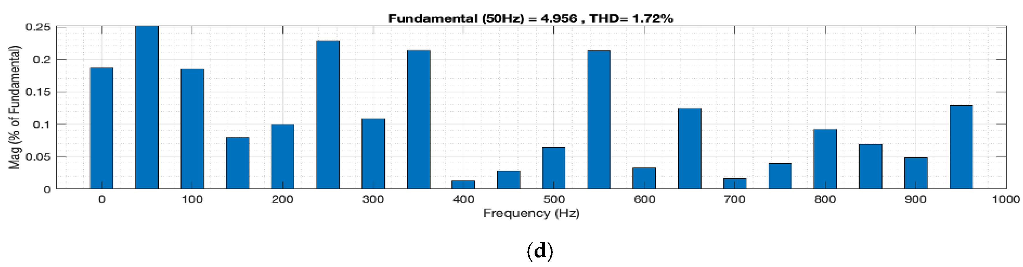
Figure 8a shows that the current output wave is good despite a small ripple caused by the shunt capacitor switching and the nature of the PI controllers’ failure for nonlinear variation. This can only be achieved by designing the parameters with the required size in consideration. It was possible to improve THD by increasing the filtering capacitor; however, this would cause heating on the system, which would increase losses. Additionally, maintaining the load current optimal and managing the response due to load variation and resonance is difficult as seen in various results [29,30]. The current wave shape in Figure 8c, on the other hand, reduces the ripple effect, improves the load imbalance, and remains stable under all conditions. This all shows the robustness of the fuzzy-influenced PI controller. As the fuzzy-tuned PI controller uses the feedback controller’s intelligence, which gives the output back to compare it with the referenced difference of input, it will have a continuous re-adjustment of the output error, and this consequently improves the fuzzy decision. As a result, the THD of the fuzzy controlled output in Figure 8d is lower than that of the PI controlled output in Figure 8b.

4.3. Comparison with Other Authors

Different authors have approached different techniques to remove the system harmonics. Some of the researchers’ work presented in

Table 4. Designed HPF performance compared to other authors’ work.

Method	THD (%)		Compensation (%)
	Unbalanced Systems
	Before Compensation	After Compensation
Fuzzy-tuned PI HPF	26.62	1.72	93.54
PI controlled HPF	26.62	4.08	84.67
PI [29]	12.97	1.13	91.28
FO [30]	11.90	2.18	81.68
Deadbeat [1]	29.9	9.4	68.56
per phase HAPF [7]	28.5, 27.6, 25.6	0.91, 0.91, 0.92	96.8, 96.7, 96.4
PPFO [30]	11.90	2.06	82.69
PSO [30]	11.90	2.18	81.26
HSO [30]	11.90	3.42	71.26

is discussed here. As seen from the table, the harmony search optimization (HSO), particle swarm optimization (PSO), firefly optimization (FO), and predator-prey based firefly optimization (PPFO) [29] methods were used to remove harmonics with a THD of 11.90. After applying each optimization technique aimed to find the minimum harmonic, the authors discovered THD values of 3.42, 2.18, 2.18, and 2.06.

However, since the system changes dynamically and these are iterative solutions for minimum value, this requires time for iteration. The system could be forced to start a new iteration before finding the optimal solution. Consequently, the findings could be unstable and could be even worse. The article presented in [7] resolved the content of the harmonic with a hybrid filter. The authors addressed the per phase content of harmonics from THD of 28.5, 27.6, and 25.6 to THD of 0.91, 0.91, and 0.92, which is remarkable. However, the PI controller needs accurate mathematical modeling and only controls when the changes that happen are linear.

Since the PI controller, as the name implies is effective for proportional variations in a system with many nonlinear circuit parameters that the authors used for filtering, it would never remain steady or the changes would not all be proportional. The PI controllers failed to monitor the dynamic changes and the effect of resonance this time. Other interesting changes in harmonic filtering are also seen in [29,30]. These authors also used a PI controller, and the test results showed the THD was successfully reduced to 1.13 and 2.18. However, apart from the natural PI character and the reason of failure during system behavior, as happened in many studies, the authors did not consider the rise of current more than nine times under normal conditions, which shows that the filtering circuit is actually acting as a load. This would also affect the entire performance during a higher resonance state, where circuit breakers would consider it as a fault current and break the line.

$$\mathrm{Compensation}(\%)=\frac{{\%\mathrm{THD}}_{\mathrm{BF}}-{\%\mathrm{THD}}_{\mathrm{AF}}}{{\%\mathrm{THD}}_{\mathrm{BF}}}\times 100\%$$

(41)

where ${\%\mathrm{THD}}_{\mathrm{BF}}$ and ${\%\mathrm{THD}}_{\mathrm{AF}}$ are the percentage total harmonics distortion before and after filtering, respectively.

This design, unlike earlier ones, addresses the rise of the current both under normal and variable loads and as a consequence of resonance effects, while taking them into consideration. Table 4 shows that while the harmonic filtering performance of both PI and fuzzy-tuned PI results with respect to compensation percentage was higher than most, the fuzzy-tuned PI controller remained superior both in compensating percentage and distorting the system harmonic where the performance was measured using (41).

5. Conclusions

In this paper, design improvements of both active and passive filters were presented. In the active filter design improvement, while the induced voltage in the unbalanced phase was considered to improve others’ work, the effect of circuit resonance due to the active filter part was also considered in the design of the passive filter. The sizing of the parameter was derived with the limiting criteria of resonance frequency, where the resonance frequency was computed from the first derivative of the circuit transfer function to determine the maximum amount of circuit resonance. On the other hand, to improve the controlling capacity with regard to nonlinear load variation, the fuzzy-tuned PI controller was designed, and the performance was presented in comparison with the traditional PI controller.

The overall performance of the designed system was tested using MATLAB Simulink^®. To consider the effect of distribution load variation with nonlinear load, an extra unbalanced load was imposed and removed during the simulation. The output wave from the DC voltage showed that, while the PI controlled output produces spikes with each load switch, the fuzzy-tuned PI controller, despite load variation and resonance effects, due to the ability of fuzzy control learning from the reasoning con-sequence of the input–output variations, continued straight and remained unaffected by load switching.

Furthermore, the grid current simulation output with the fuzzy-tuned PI controller was smoother and more sinusoidal than the ripple-affected PI controlled output, which generalizes that the overall design of the HPF with fuzzy-tuned PI control performed better in suppressing harmonics. As a result, the THD of the system harmonics was reduced from 26.62 to 4.08 and 1.72 after being filtered by the designed PI controller and fuzzy-tuned PI controller, respectively.

The authors would like to advance this research with the comparison of other control methods, experiments, and possible mathematical improvements in future work.

References

- Sou, W.-K.; Choi, W.-H.; Chao, C.-W.; Lam, C.-S.; Gong, C.; Wong, C.-K.; Wong, M.-C. A deadbeat current controller of LC-hybrid active power filter for power quality improvement. IEEE J. Emerg. Sel. Top. Power Electron. 2019, 8, 3891–3905. [Google Scholar] [CrossRef]
- Antunes, H.M.A.; Pires, I.A.; Silva, S.M. Evaluation of series and parallel hybrid filters applied to hot strip mills with cycloconverters. IEEE Trans. Ind. Appl. 2019, 55, 6643–6651. [Google Scholar] [CrossRef]
- Terriche, Y.; Mutarraf, M.U.; Golestan, S.; Su, C.-L.; Guerrero, J.M.; Vasquez, J.C.; Kerdoun, D. A hybrid compensator configuration for var control and harmonic suppression in all electric shipboard power systems. IEEE Trans. Power Deliv. 2020, 35, 1379–1389. [Google Scholar] [CrossRef]
- Xue, C.; Zhou, D.; Li, Y. Hybrid model predictive current and voltage control for LCL-filtered grid-connected inverter. IEEE J. Emerg. Sel. Top. Power Electron. 2021, 9, 5747–5760. [Google Scholar] [CrossRef]
- Xu, C.; Dai, K.; Chen, X.; Peng, L.; Zhang, Y.; Dai, Z. Parallel resonance detection and selective compensation control for SAPF with square-wave current active injection. IEEE Trans. Ind. Electron. 2017, 64, 8066–8078. [Google Scholar] [CrossRef]
- Wang, Y.; Xu, J.; Feng, L.; Wang, C. A novel hybrid modular three level shunt active power filter. IEEE Trans. Power Electron. 2018, 33, 7591–7600. [Google Scholar] [CrossRef]
- Salmerón, P.; Litrán, S.P. A control strategy for hybrid power filter to compensate four wires three-phase systems. IEEE Trans. Power Electron. 2010, 25, 1923–1931. [Google Scholar] [CrossRef]
- Zouidi, A.; Fnaiech, F.; Al-Haddad, K. Voltage source inverter based three-phase shunt active power filter: Topology, modeling and control strategies. In Proceedings of the 2006 IEEE International Symposium on Industrial Electronics, Montreal, QC, Canada, 9–13 July 2006. [Google Scholar]
- Daftary, D.; Shah, M.T. Design and analysis of hybrid active power filter for current harmonics mitigation. In Proceedings of the 2019 IEEE 16th India Council International Conference (INDICON), Rajkot, India, 13–15 December 2019. [Google Scholar]
- Inzunza, R.; Akagi, H. A 6.6-kV transformerless shunt hybrid active filter for installation on a power distribution system. IEEE Trans. Power Electron. 2005, 20, 893–900. [Google Scholar] [CrossRef]
- Wu, W.; He, Y.; Blaabjerg, F. An LLCL power filter for single-phase grid-tied inverter. IEEE Trans. Power Electron. 2012, 27, 782–789. [Google Scholar] [CrossRef]
- Zhou, X.; Cui, Y.; Ma, Y. Fuzzy linear active disturbance rejection control of injection hybrid active power filter for medium and high voltage distribution network. IEEE Access 2021, 9, 8421–8432. [Google Scholar] [CrossRef]
- Shao, Y.; Yao, Y.; Liu, H.; Lv, R.; Zan, P. Power harmonic detection method based on dual HSMW window fft/apfft comprehensive phase difference. In Proceedings of the 40th Chinese Control Conference, Shanghai, China, 26–28 July 2021. [Google Scholar]
- Mohamed, I.S.; Rovetta, S.; Do, T.D.; Dragicevic, T.; Diab, A.A.Z. A neural network-based model predictive control of three-phase inverter with an output LCL filter. IEEE Access 2019, 7, 124737–124749. [Google Scholar] [CrossRef]
- Hao, Z.; Wang, X.; Cao, X. Harmonic control for variable-frequency aviation power system based on three-level NPC Converter. IEEE Access 2020, 8, 132775–132785. [Google Scholar] [CrossRef]
- Suresh, Y.; Panda, A.K.; Suresh, M. Real time implementation of adaptive fuzzy hysteresis-band current control technique for shunt active power filter. IET Power Electron. 2012, 5, 1188–1195. [Google Scholar] [CrossRef] [Green Version]
- Choi, U.; Lee, K.B. Space vector modulation strategy for neutral point voltage balancing in three-level inverter systems. IET Power Electron. 2013, 6, 1390–1398. [Google Scholar] [CrossRef]
- Akagi, H.; Kanazawa, Y.; Nabae, A. Instantaneous reactive power compensators comprising switching devices without energy storage components. IEEE Trans. Ind. Appl. 1984, IA-20, 625–630. [Google Scholar] [CrossRef]
- Herrera, R.S.; SalmerÓn, P.; Kim, H. Instantaneous reactive power theory applied to active power filter compensation: Different approaches, assessment, and experimental results. IEEE Trans. Ind. Electron. 2008, 55, 184–196. [Google Scholar] [CrossRef]
- Willems, J.L. A new interpretation of the Akagi-Nabae power components for nonsinusoidal three-phase situations. IEEE Trans. Instrum. Meas. 1992, 41, 523–527. [Google Scholar] [CrossRef]
- Kazmierkowski, M.P.; Jasinski, M.; Wrona, G. DSP-based control of grid-connected power converters operating under grid distortions. IEEE Trans. Ind. Inform. 2011, 7, 204–211. [Google Scholar] [CrossRef]
- Hong, L.; Shu, W.; Wang, J.; Mian, R. Harmonic resonance investigation of a multi-inverter grid-connected system using resonance modal analysis. IEEE Trans. Power Deliv. 2019, 34, 63–72. [Google Scholar] [CrossRef]
- Lu, M.; Wang, X.; Loh, P.C.; Blaabjerg, F. Resonance interaction of multiparallel grid connected inverters with LCL Filter. IEEE Trans. Power Electron. 2017, 32, 894–899. [Google Scholar] [CrossRef]
- Enslin, J.H.R.; Heskes, P.J.M. Harmonic interaction between a large number of distributed power inverters and the distribution network. IEEE Trans. Power Electron. 2004, 19, 1586–1593. [Google Scholar] [CrossRef]
- Kim, H.-S.; Sul, S.-K. Resonance suppression method for grid-connected converter with LCL filter under discontinuous PWM. IEEE Access 2021, 9, 124519–124529. [Google Scholar] [CrossRef]
- Liserre, M.; Blaabjerg, F.; Hansen, S. Design and control of an LCL-filter-based three-phase active rectifier. IEEE Trans. Ind. Appl. 2005, 41, 1281–1291. [Google Scholar] [CrossRef]
- Chitsazan, M.A. A new approach to LCL filter design for grid-connected PV sources. Am. J. Electr. Power Energy Syst. 2017, 6, 57. [Google Scholar] [CrossRef] [Green Version]
- Li, H.-X.; Zhang, L.; Cai, K.-Y.; Chen, G. An improved robust Fuzzy-PID controller with optimal fuzzy reasoning. IEEE Trans. Syst. Man Cybern. Part B (Cybernetics) 2005, 35, 1283–1294. [Google Scholar] [CrossRef] [Green Version]
- Imam, A.A.; Kumar, R.S.; Al-Turki, Y.A. Modeling and simulation of a PI controlled shunt active power filter for power quality enhancement based on P-Q theory. Electronics 2020, 9, 637. [Google Scholar] [CrossRef]
- Mahaboob, S.; Ajithan, S.K.; Jayaraman, S. Optimal design of shunt active power filter for power quality enhancement using predator-prey based firefly optimization. Swarm Evol. Comput. 2019, 44, 522–533. [Google Scholar] [CrossRef]
Figure 1.
LCL-HPF system structure.
Figure 2.
Equivalent circuit of the LCL-HPF filter.
Figure 3.
The input–output membership and output surface for a fuzzy control system (a) the membership function of the input VDC error control; (b) the membership function of the fuzzy controlled change () input; (c) the membership function of the fuzzy controlled errors; and (d) the membership function rules of the fuzzy control output 3D surface view.
Figure 4.
The arrangement of the (a) fuzzy control structure and (b) fuzzy control model.
Figure 5.
Parameter and working principle of the LCL-HPF (a) active and passive filter parameter computation and (b) the designed filter working algorithm.
Figure 6.
Load current and THD (a) variable load current wave shape and (b) system THD prior to filtering.
Figure 7.
The switching current and DC voltage performance (a) the PI controller filtering output current, (b) the fuzzy-tuned PI controller filtering current wave shape, (c) the shunt capacitor voltage response with PI controller, and (d) the shunt capacitor voltage response with fuzzy-tuned PI controller.
Figure 8.
Grid current and the THD after HPF. (a) Grid current waveform after a PI-controlled HPF addition, (b) THD after PI controlled HPF has been added to the filter, (c) the grid current output wave shape after incorporating the fuzzy-tuned PI controller into the HPF circuit, and (d) the THD of the fuzzy-assisted PI controlled HPF.