Abnormal Detection for Running State of Linear Motor Feeding System Based on Deep Neural Networks

Abstract

Because the linear motor feeding system always runs in complex working conditions for a long time, its performance and state transition have great randomness. Therefore, abnormal detection is particularly significant for predictive maintenance to promptly discover the running state degradation trend. Aiming at the problem that the abnormal samples of linear motor feed system are few and the samples have time-series features, a method of abnormal operation state detection of a linear motor feed system based on normal sample training was proposed, named GANomaly-LSTM. The method constructs an encoding-decoding-reconstructed encoding network model. Firstly, the time-series features of vibration, current and composite data samples are extracted by the long short-term memory (LSTM) network; Secondly, the three-layer fully connected layer is employed to extract potential feature vectors; Finally, anomaly detection of the system is completed by comparing the potential feature vectors of the two encodings. An experimental platform of the X-Y two-axis linkage linear motor feeding system is built to verify the rationality of the proposed method. Compared with other classical methods such as GANomaly and GAN-AE, the average AUROC index of this method is improved by 17.5% and 9.3%, the average accuracy is enhanced by 11.6% and 15.5%, and the detection time is shortened by 223 ms and 284 ms, respectively. GANomaly-LSTM has successfully proved its superiority for abnormal detection for running state of linear motor feeding systems.

1. Introduction

As a key component of position tracking and positioning control for high-end CNC equipment, robots and precision motion platforms [1], a linear motor feeding system has the characteristics of multi-domain coupling, high integration of functions and dynamic and changeable performance. The complexity of electromechanical thermomagnetic coupling increases the probability of performance degradation, functional failure and malfunction. At the same time, under the combined effect of high-speed operation, mechanical friction, wear, high temperature and corrosion for a long time, unforeseen abnormal states and failures will occur. Therefore, abnormal detection, timely identification of abnormal states and predictive maintenance of the linear motor feeding system are particularly important.

With the increasing complexity of industrial equipment, the traditional way of replacing parts on schedule or judging abnormalities based on human experience can no longer meet the demand. Currently, the methods for anomaly detection of complex mechanical equipment are mainly divided into statistical-based, graph-based and machine learning-based approaches.

Statistical-based approaches need to collect historical data from equipment for statis-tical analysis to form a large number of normal data samples and abnormal data samples, and detect anomalies by extracting their features. Statistical models for anomaly detection mainly include the Gaussian model, regression model and expectation maximization model. Wang et al. [2] adopted an anomaly detection method based on the Gaussian model, which used the Gaussian model to represent the normal distribution of the data, and then scored the data according to the similarity between the model and the data. While this method can only be applied to data sets with a single attribute, and the distribution law of the data set needs to be known in advance. It is not applicable to the processing of high-dimensional data. Jin et al. [3] developed a bearing anomaly detection and fault prediction method based on an autoregressive model. The abnormality threshold was set by the attributes of Box-Cox transformation and Gaussian distribution. When the health index of the test data was greater than the abnormality threshold, it was judged as abnormal data. However, the threshold set often had errors, and an accurate dividing line between abnormal and normal data cannot be obtained. Liu et al. [4] proposed a novel filter based on an expectation-maximization model to identify anomalies in time-series data. The disadvantage of this model was the absolute dependence on the abnormal threshold. Statistical-based approaches do not re-quire establishing precise system models, and the algorithms are simple and easy to implement. However, this method is unsuitable for dealing with multivariate data, and the lack of fault data samples will lead to inaccurate detection results.

Graph-based approaches abstract entities as vertices and relationships as edges connecting vertices in the graph, providing a powerful means to express the complex relationships between entities. The traditional graph anomaly detection technology mainly obtains the graph statistical information through statistics and probability methods for anomaly detection. The shortcomings of these kind of methods are slow con-tent collection and low efficiency. In recent years, graph-based anomaly detection techniques have gradually developed, mainly used to solve the problem of anomaly detection in complex networks [5,6]. The key to this method is learning the correlation between different graph data. However, the nodes of objects in graph data are connected by edges, resulting in often complex correlations among the nodes. Recently, there is no precedent for their application in linear motor feeding systems.

Machine learning-based approaches include distance-based, deviation-based, density-based, and deep learning-based approaches.

The distance-based methods calculate point or collective anomalies by measuring the distances between data points and adjacent points or between data sequences and adjacent sequences. Objects farther away from others are considered anomalies. Zhang et al. [7] proposed a k-nearest neighbor (KNN) anomaly detection algorithm. It calculated the anomaly score by calculating the average distances between all K adjacent nodes. Li et al. [8] presented a clustering-based anomaly detection approach. The similarity of the time-series was evaluated by using the Euclidean distance function in the original feature space to judge whether the amplitudes are abnormal or not. The advantage of distance-based methods is that they are very efficient and easy to implement when dealing with low-dimensional data. The disadvantage is that they are expensive with regard to calculating distances between multivariable data sets.

The deviation-based approach uses models to make predictions on time-series data. If the deviation between the predicted value and the actual value of a data point exceeds a certain threshold, the data point is judged as abnormal. Li et al. [9] proposed a prediction-based anomaly detection method for time-series. An exception is detected by setting a threshold. Outliers are identified when the deviation between the predicted and actual values is greater than the threshold. Zhou et al. [10] proposed a deviation-based approach to anomaly detection for combined models; whether the sequence is abnormal is judged by the comparison. The abnormal score of a fragment in the sequence is calculated according to the deviation, and then the average score of all fragments is obtained. However, this approach is less effective for datasets with unknown prior knowledge and high-dimensional multivariate data.

The density-based approaches identify outliers by calculating the density of data objects. When the local density of the data object is different from the adjacent area, it will be dis-criminated as an outlier. Classical algorithms based on this method are Local Outlier Factor (LOF) and INFLuenced Outlierness (INFLO). Abdulghafoor et al. [11] proposed a density-based outlier detection method. This method compared the density of the observed object with the surrounding local density, using the LOF as a variable to measure the outliers. When the INFLO [12] algorithm estimates the density distribution of objects, it considers the relationship between the neighborhood and the reverse neighborhood of the object to rank the outliers. The higher the INFLO value of the detected object, the more likely it is to be an outlier. The advantage of the density-based method is that it can detect not only global outliers but also local outliers. The disadvantage is that time correlation on time step is not considered. Therefore, this method cannot be effectively used for anomaly detection of multivariate time-series data.

In recent years, deep learning has been widely adopted in image recognition, object detection, semantic analysis, etc. In order to efficiently and accurately mine effective state information from big mechanical data, deep learning has also been popularly applied in mechanical fault diagnosis [13]. Hoang et al. [14] proposed a convolutional neural network (CNN) that used vibration signals to detect bearing faults. Shao et al. [15] designed a stack transfer autoencoder and used the particle swarm optimization algorithm for fault diagnosis of rotating machinery. Jiang et al. [16] put forward the deep belief networks (DBNs), which directly extracted fault-related features from the original vibration signal and current signal, and the two features for fault diagnosis of a wind turbine gearbox. However, the above deep learning methods require a large amount of historical data in different health states for training. In the operation of linear motor feeding systems, data samples are often only available for normal operating conditions, but not for fault conditions. Due to the insufficient failure samples of the linear motor feed system, the deep learning method is difficult to apply. The reasons for this phenomenon are as follows: (1) The fault situation is far less than the normal situation, and it is difficult to collect fault data; (2) Even if the fault data can be collected, it takes a long time and costs a lot; (3) Some fault data cannot be measured under laboratory conditions. The data generated by the linear motor feeding system is mostly time-series data, with apparent time and sequence features, such as vibration signal and current signal. Collecting abnormal samples for linear motor feeding systems is challenging under current conditions. Therefore, it is an exigent issue to realize the abnormal detection of the running state of the linear motor feeding system in the absence of fault samples.

Recently, the generative adversarial network (GAN) has brought new hope for solving the problem of insufficient samples. GAN is a new network structure that was proposed by Goodfellow [17] in 2014, which is an unsupervised feature learning algorithm based on the idea of adversarial training. The method has been extensively used in anomaly detection because it can use adversarial learning of sample representations for anomaly inference [18]. With the continuous improvement of generative adversarial ideas, many improved generative adversarial networks have been derived, such as the efficient GAN-based anomaly detection (EGBAD) network [19], deep convolutional generative adversarial network (DCGAN) [20], anomaly generative adversarial networks (AnoGAN) [21], et al. These improved GANs can generate training samples by learning the probability distribution of real data, so as to solve the problem of insufficient fault samples in the process of model training. Wang et al. [22] achieved a fault diagnosis approach combining GAN and a stacked denoising autoencoder (SDAE) to generate fault data for the problem of a small number of fault samples in planetary gearboxes. Mao et al. [23] combined GAN with the stacked denoising auto encoder (SDAE) to solve the problem of data imbalance in bearing fault diagnosis. Gao et al. [24] proposed a data augmentation method based on the Wasserstein generative adversarial network with gradient penalty (WGAN-GP) and verified the feasibility of generating fault samples on three datasets. The above studies show that GAN can generate fault samples, dramatically expanding the range and diversity of generated data samples. However, the above models still require a small amount of fault samples, and it is difficult to complete training with a complete lack of them.

Given the above particular situation, Akcay et al. [25] proposed a GANomaly method, which can complete the training of the model without abnormal samples. Subsequently, Akcay et al. [26] further achieved a Skip-GANomaly detection method for images based on GANomaly, which only used normal samples for training. Luo et al. [27] proposed a geological image anomaly detection method based on GANomaly. Liu et al. [28] applied an anomaly detection method based on GANomaly and CNN, which adopted normal time-series data samples for training, and encodes them into two-dimensional images using the Gramian Angular Field (GAF) method. The abnormal detection of vibration signals of long-span bridges was realized, and a good detection effect was achieved. GANomaly is an anomaly detection method commonly used in images. When dealing with time-series data, the gradient disappearance and gradient explosion problems are its traditional limitations, influenced by the choice of activation function and the error back propagation method [29]. The deeper the network layer, the more obvious the problem becomes [30]. Therefore, it is necessary to find an efficacious method.

The long-short-term memory (LSTM) network includes a memory unit, gate structure and attention mechanism, which can effectively solve the aforesaid problems. Methods based on LSTM have excellent anomaly detection capability for time-series data [31]. Li et al. [32] adopted a method based on stacked autoencoders (SAE) and LSTM networks for anomaly detection in vibration signals of rotating machinery. Chen et al. [33] raised an anomaly detection method for time-series data of wind turbines based on LSTM and an auto-encoder (AE) neural network. Vos et al. [34] developed a gear anomaly detection algorithm combining deep learning and LSTM. Ou et al. [35] provided a bearing state anomaly detection method based on the LSTM network. In the training process of this method, only health data was used. Bai et al. [36] used the LSTM network for fault detection of gas turbines. Aiming at the problem that the newly-run gas turbine was difficult with regard to obtaining fault data, this method only used normal data to train the network. Kong et al. [37] developed an anomaly detection method for industrial multidimensional time-series data. This method used a bi-directional LSTM with the attention mechanism in the generator and discriminator of GAN. The results indicated that the method had favorable performance in the task of anomaly detection for industrial time-series data.

On the one hand, GANomaly can complete model training without abnormal samples. On the other hand, LSTM can avoid gradient disappearance and gradient explosion when training time-series data.

Therefore, combining the advantages of GANomaly and the LSTM neural network, an abnormal detection method for the running state of the linear motor feeding system is proposed in this paper. Based on the analysis of the factors affecting the running state of the linear motor feeding system, the abnormal detection network framework is designed by taking vibration signals and current signals as the original data. Firstly, the LSTM network is used to extract the input sample time-series features, then the three-layer fully connected layer is employed to extract potential feature vectors. Secondly, the anomaly score of the input sample is obtained by comparing the difference between the latent feature vectors obtained by the two encodings. The relationship between the abnormal score value and the threshold value is used to judge whether the input sample is abnormal, so as to realize the abnormal detection of the running state of the linear motor feeding system. Finally, the experimental platform of the X-Y two-axis linked linear motor feeding system is built to validate the proposed method experimentally.

The main contributions of this article are listed below:

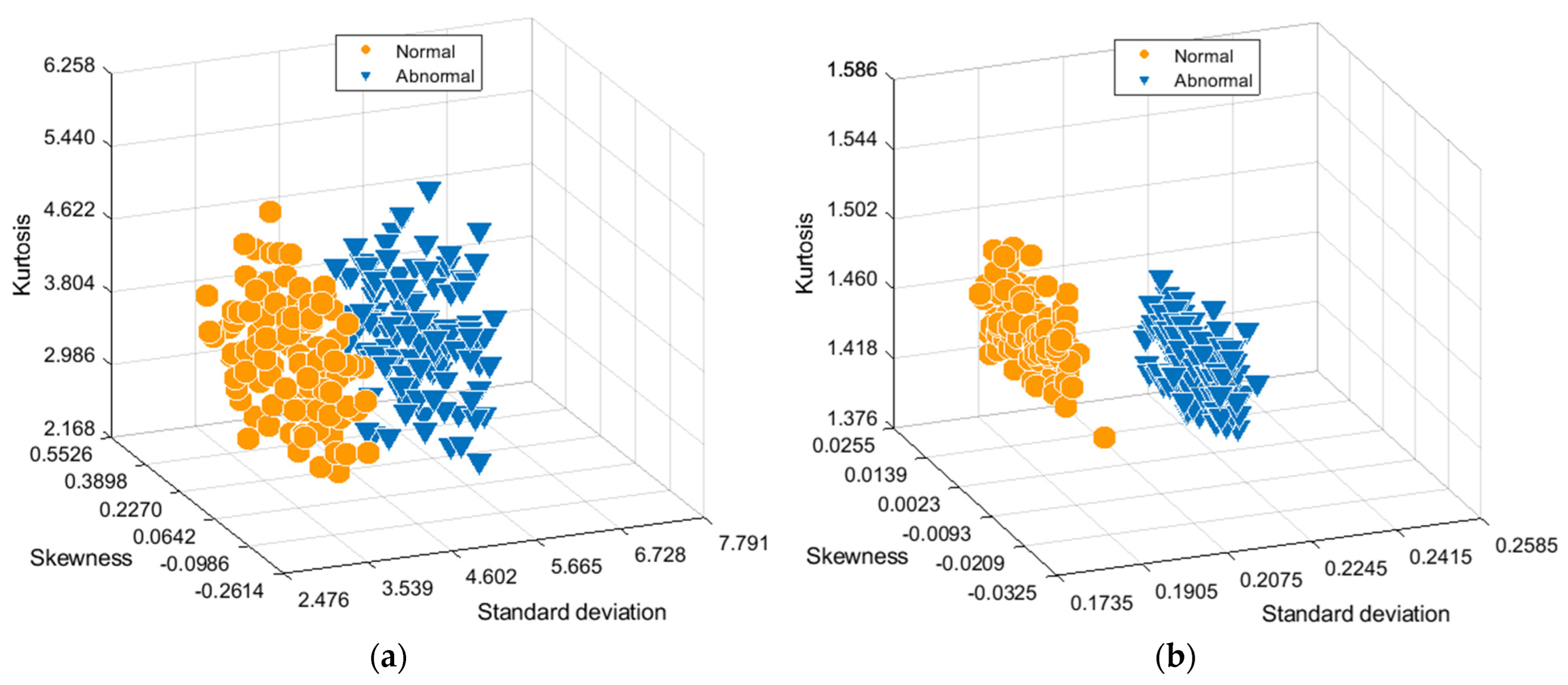
• A GANomaly-LSTM method is proposed, which can effectively avert the teasers of gradient disappearance and gradient explosion during the course of training time-series data, and the extracted features can achieve a good clustering effect.
• This method can realize anomaly detection in the absence of abnormal sample training.
• The proposed model performs well in anomaly detection of phase-missing current signals and vibration signals, verified under three input conditions.
• A mass of experiments have been actualized, and the results indicate that the proposed method achieves excellent advantages in effectiveness and performance compared with other classical methods.

The rest of this paper is organized as follows. Section 2 provides a theoretical introduction to the GANomaly-LSTM method. Section 3 builds the experimental platform for the X-Y two-axis linked linear motor feeding system and describes the process of experimental setup, data acquisition and feature extraction. Section 4 provides a detailed analysis of the experimental results. In Section 5, we draw conclusions and discuss directions for future work.

2. Anomaly Detection Model of Linear Motor Feeding System

2.1. Factors Affecting the Running State of Linear Motor Feeding System

The feeding system of the X-Y two-axis linkage linear motor is employed as the research object. The X-axis is cross orthogonal to the Y-axis, and the Y-axis is located above the X-axis and coupled with the X-axis stator. Factors affecting the running state of the linear motor feeding system mainly include three aspects: (1) Abnormal vibration. Because the linear motor feeding system has no intermediate transmission link, the mechanical damping of the linear motor is small, so the vibration is difficult to be effectively attenuated, which seriously affects the running state of the feeding system. At the same time, the vibration in the processing process is one of the critical factors affecting the machining accuracy, which will reduce not only the surface quality of the workpiece and the dynamic precision of the machine tool but also the productivity [38]; (2) Motor overheating. Severe wear of motor guides will lead to overheating, and increase stator resistance, further leading to abnormal acceleration changes of the linear motor, ultimately affecting the operation state of the feeding system; (3) Excessive load. The vibration will accelerate the wear of power transmission components and overload the transmission and machine tool structures, resulting in the current fluctuation of the linear motor feeding system, thus leading to the change of the operating state [1]. It can be seen that acceleration and current are the two key factors to reflect the evolution of the running state of the linear motor feeding system. Therefore, vibration signals and current signals of the experimental platform under different working conditions are used as the original acquisition time-series data in this paper.

2.2. Anomaly Detection Model

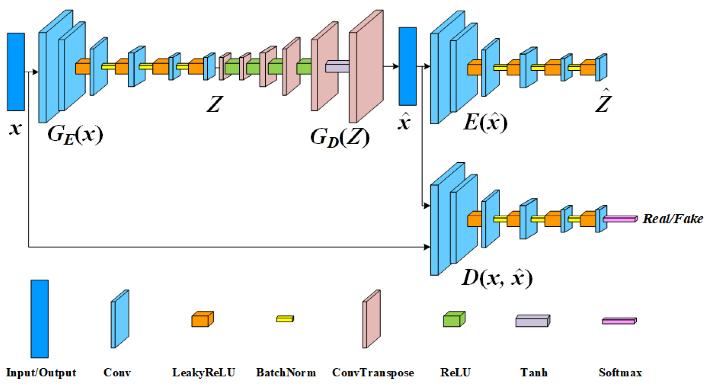
2.2.1. The Structure of GANomaly

The GANomaly method adds an adversarial learning strategy to the autoencoder generation model, which is an anomaly detection method that compares the potential features of sample coding. GANomaly determines whether a data sample is abnormal or not based on the difference between the potential feature vector $Z$ and $\hat{Z}$ obtained from the two encoders. GANomaly has strong robustness and anti-noise interference capability, requiring only a small number of abnormal samples or no abnormal samples during learning and training [39].

The GANomaly model framework consists of three parts: a generator, a reconstructed encoder, and a discriminator. The network structure of GANomaly is shown in Figure 1. The encoder $G_E\left(x\right)$ and decoder $G_D\left(Z\right)$ in Figure 1 are collectively referred to as generators. The input data $x$ passes through the encoder $G_E\left(x\right)$ to obtain the latent feature vector $Z$, then passes through the decoder $G_D\left(Z\right)$ to obtain the reconstructed data $\hat{x}$. The reconstructed encoder $E\left(\hat{x}\right)$ encodes the reconstructed data $\hat{x}$ again to get the potential feature vectors $\hat{Z}$ of the reconstructed data. The idea of adversarial learning is introduced in discriminator $D(x,\hat{x})$ to distinguish the differences between the original input data $x$ and the reconstructed data $\hat{x}$. It determines original input data $x$ to be true and reconstructed data $\hat{x}$ to be false. The discriminator is designed as a network with the same structure as the encoder in the generator. Meanwhile, the gap between the reconstructed and original input data is continuously optimized.

In the training stage, the whole model is trained with normal samples. When the model is inputted with an abnormal sample in the testing stage, there is a certain difference between the potential feature vectors obtained by the encoder and the reconstructed encoder because the decoder is trained by normal samples. When the difference is greater than a certain threshold, the input sample is identified as abnormal [40].

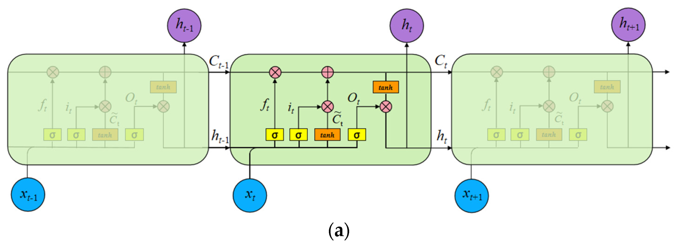
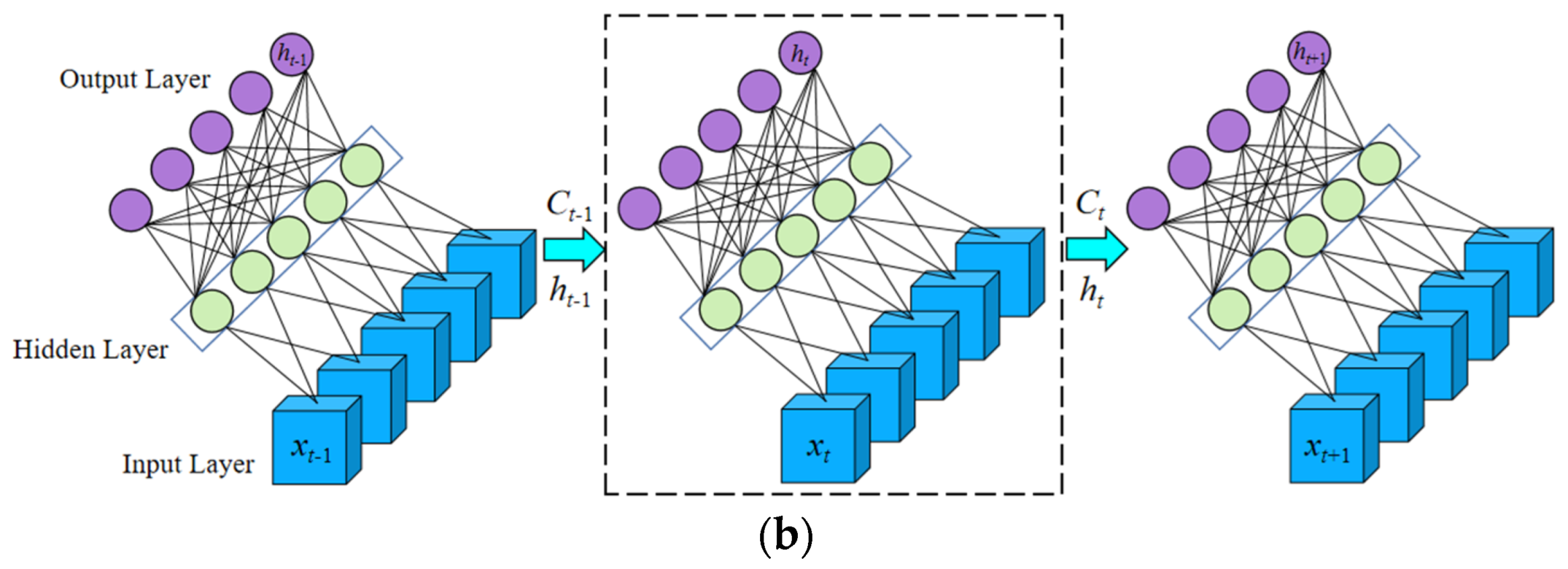
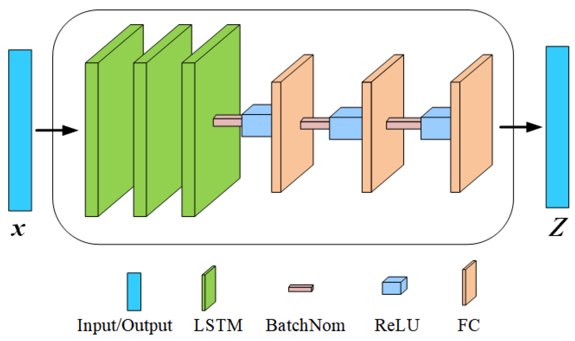
2.2.2. The Structure of LSTM

LSTM is a special RNN which can solve the long-term dependency problem well [41]. The standard RNN has only one tanh layer, while the internal structure of LSTM is more complex, consisting of four neural network layers: forgetting gate, input gate, cell state and output gate (as shown in Figure 2) [42]. The advantages and limitations of RNN and LSTM are listed in

Table 1. Advantages and limitations of RNN and LSTM.

	LSTM	RNN
Advantages	1. The problem of gradient disappearance and gradient explosion can be overcome when training long sequence data; 2. Able to learn long-term dependence; 3. Simple to implement.	1. Train the time-series data; 2. The network is simple and easy to operate.
Limitations	1. Because of the large amount of computation in network training, high performance computers are needed.	1. Cannot process long time-series data; 2. There are problems of gradient disappearance and gradient explosion.

.

The first layer is “forget gate”, and its input is h_t−1 and x_t, mainly focusing on selectively forgetting the information of h_t−1. Through σ, a sigmoid activation function, the output f_t is the value within the interval of [0, 1]. “0” represents that the state is inactive and all information is forgotten, while “1” represents the opposite. The sigmoid activation function is shown in Figure 3a. The equation of the forget gate is as follows:

$$f_t=\sigma \left(W_f \left[h_{t-1}{,x}_t\right]{+b}_f\right)$$

(1)

where σ is the sigmoid activation function; x_t is the input at time t; h_t−1 is the output of the time t−1; and W_f and b_f are the weight and bias parameters of the forget gate, respectively.

The second layer is “input gate”. It determines what information of the cell state needs to retain. The input gate includes the sigmoid layer and tanh layer. The sigmoid layer determines what information needs to be updated at the input gate. The tanh layer creates a matrix to add to the cell state. The tanh activation function is shown in Figure 3b. The input of the input gate is h_t−1 and x_t, so that the equation can be expressed as:

$$i_t=\sigma \left(W_i \left[h_{t-1}{,x}_t\right]{+b}_i\right)$$

(2)

$${\tilde{C}}_t=\mathit{tanh}\left(W_C\left[h_{t-1},x_t\right]+b_C\right)$$

(3)

where W_i is the weight of sigmoid function in the input gate; b_i is the bias parameter of sigmoid function; W_C is the weight of tanh function; b_C is the bias parameter of the tanh function.

The third layer is “cell state”. It can update the cell state C_t−1 to the current cell state C_t, which can be expressed as:

$$C_t=f_t{C}_{t-1}+i_t{\tilde{C}}_t$$

(4)

The fourth layer is “out gate”. It influences the output of the current cell state. The sigmoid function layer determines which parts should be updated. And the tanh function can operate on the cell state C_t, so that tahn(C_t) ranges (−1, 1). Multiply the output of the sigmoid function, then the part h_t will be gotten. The output gate equation can be expressed as:

$$o_t=\sigma \left(W_o\left[h_{t-1}{,x}_t\right]{+b}_o\right)$$

(5)

$$h_t{=o}_t·\mathit{tanh}\left(C_t\right)$$

(6)

where o_t is the output gate; W_o and b_o are the weight and the bias parameter, respectively; h_t is the output of the current cell state and the input of the next state as well.

Besides, Rectified Linear Unit (ReLU) is also a popular activation function, as shown in Figure 3c.

2.2.3. Proposed Method

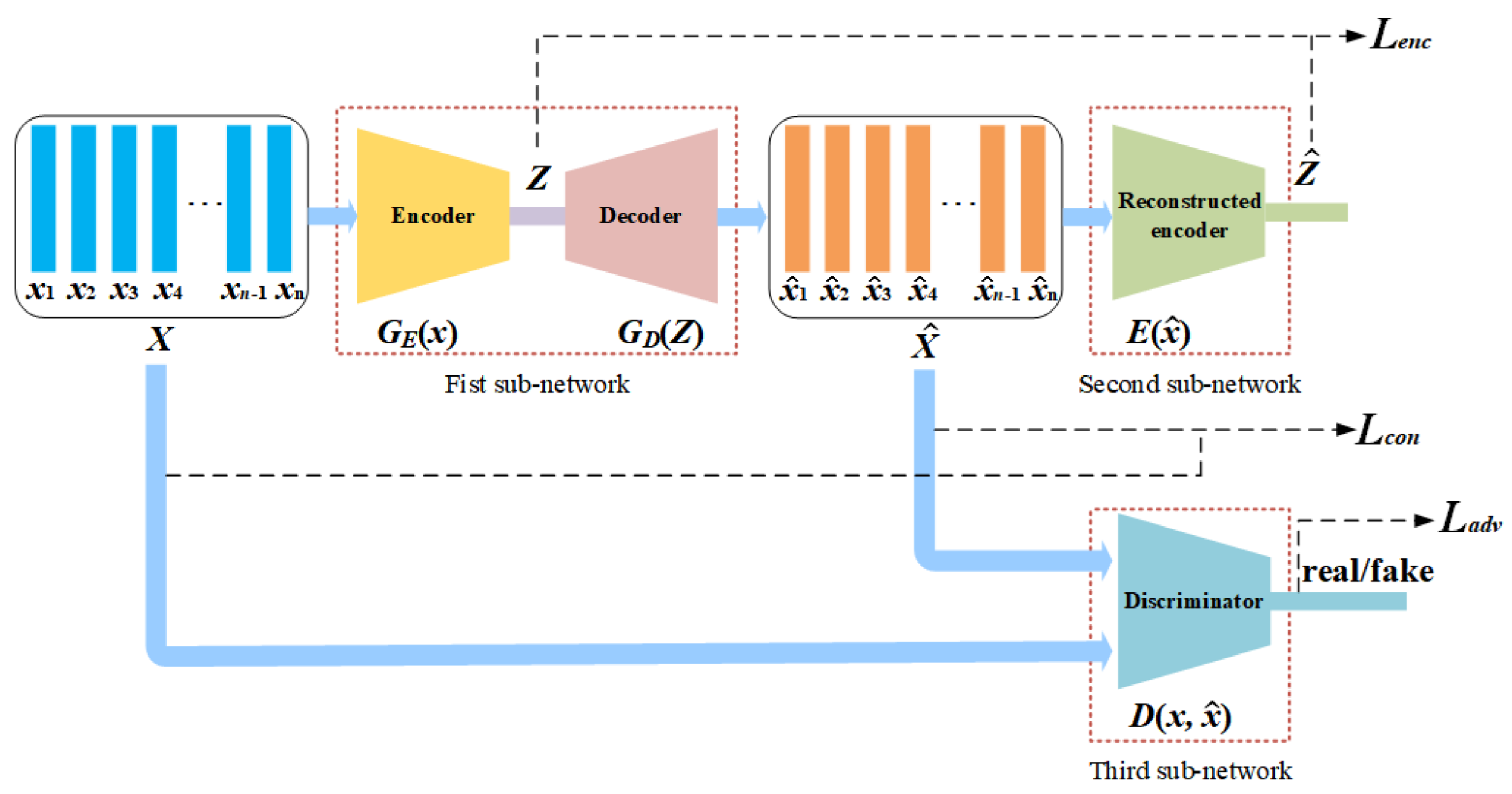
The Structure of GANomaly-LSTM

Based on the theories of the GANomaly and LSTM network, an anomaly detection method for linear motor feeding system based on GANomaly-LSTM is proposed. As shown in Figure 4, the GANomaly-LSTM network structure comprises three sub-networks: the generation network, the reconstructed encoder network and the discriminant network.

The first sub-network is the generative network, including encoder $G_E\left(x\right)$ and decoder $G_D\left(Z\right)$. The encoder $G_E\left(x\right)$ structure is expressed in Figure 5. A three-layer LSTM is used to extract time-series features of samples, and then a three-layer fully connected layer is used to extract potential feature vectors. Three batch standardization layers and three rectifying linear unit (ReLU) activation functions are used to optimize the output distribution of the middle layer. The structures of decoder $G_D\left(Z\right)$ and encoder $G_E\left(x\right)$ are opposite. For the input data $x$, the latent feature vector $Z$ is obtained through the encoder $G_E\left(x\right)$, and then the reconstructed data of $\hat{x}$ is obtained through the decoder $G_D\left(Z\right)$.

The second subnetwork is the reconstructed encoder network, and by re-encoding the reconstructed data $\hat{x}$, the latent feature vector $\hat{Z}$ of the reconstructed data is obtained. In this subnetwork, the structure of the reconstructed encoder $E\left(\hat{x}\right)$ is the same as $G_E\left(x\right)$.

The third sub-network is the discriminant network, which continuously narrows the gap between the reconstructed data and the original input data by judging the original input data $x$ as true and the reconstructed data $\hat{x}$ as false. Ideally, the reconstructed data is no different from the original input data. By introducing the idea of adversarial training, the generative and discriminant networks play games. On the one hand, it improves the ability of the decoder to recover the input samples, and on the other hand, it enhances the feature extraction ability of the encoder. The discriminator $D(x,\hat{x})$ has the same structure as $G_E\left(x\right)$.

Loss Function

In the generative network, the reconstruction error loss is defined as the gap between the original input data and the reconstructed data.

$$L_{con}=|x-\hat{x}|$$

(7)

where $L_{\mathit{con}}$ is the reconstruction error loss function of the generative network.

A feature matching error is set in the discriminant network for optimization in the data feature layer.

$$L_{adv}=|f(x)-f(\hat{x})|$$

(8)

where $L_{\mathit{adv}}$ is the loss function of the discriminant network, and it specifically refers to the loss of confrontation between the generation network and the discriminant network; f is the transfer function of the model.

Ideally, for normal data, the difference between the latent eigenvector $\hat{Z}$ of the reconstructed data and the latent eigenvector $Z$ is extra small. In order to quantify and optimize this difference in the training phase, the error between latent feature vectors is introduced:

$$L_{enc}=|Z-\hat{Z}|$$

(9)

where $L_{\mathit{enc}}$ is the loss function of the latent eigenvector error of the reconstructed data.

For the entire network model, the loss function can be expressed as:

$$L_{\mathit{total}}{=\omega }_{\mathit{adv}}{L}_{\mathit{adv}}{+\omega }_{\mathit{con}}{L}_{\mathit{con}}{+\omega }_{\mathit{enc}}{L}_{\mathit{enc}}$$

(10)

where ${\omega }_{\mathit{adv}}$, ${\omega }_{\mathit{con}}$ and ${\omega }_{\mathit{enc}}$ represent the weights of $L_{\mathit{adv}}$, $L_{\mathit{con}}$ and $L_{\mathit{enc}}$, respectively.

The gradient descent method is a popular optimization algorithm in deep learning. Its basic idea is to update the parameters along the opposite direction of the gradient of the loss function about the parameters as the search direction, so that the loss function gradually decreases and finally reaches the minimum value. The gradient descent method can be divided into fixed learning rate optimization algorithms (e.g., SGD, Momentum, and NGA) and adaptive learning rate optimization algorithms (e.g., Adagrad, RMSprop, and Adam) [43].

The Adam optimization algorithm adopts the adaptive learning rate and momentum mechanism to determine the updated direction by considering the previous gradient and the current gradient together, so that the function convergence process is more stable. Moreover, the first-order moment estimation and second-order moment estimation of the gradient can be used to dynamically adjust the learning rates of different parameters to accelerate the convergence rate of the function, so as to obtain the global optimal parameters with less iterations [44]. Therefore, the Adam optimization algorithm is selected to optimize the model parameters in this paper.

Model Validation and Evaluation Criteria

After the training is complete, the model is validated using the test set. Firstly, the generative network can generate reconstructed test samples. In order to obtain the similarity between the potential feature vector $Z$ of the first encoding and the potential feature vector $\hat{Z}$ of the second encoding, the gradient descent method Adam is chosen to update continuously, and then the optimal potential feature vector will be obtained.

$${}_{\hat{Z}}^{\mathit{min}}E(Z,\hat{Z})=1-Simi(Z,\hat{Z})$$

(11)

where $\mathit{Simi}$ is the similarity function and $E$ is the error function.

Secondly, anomalies are detected using the gap between the latent feature vector after the first encoding of the test sample and the latent feature vector of the reconstructed data after the second encoding. The anomaly score $A\left(X\right)$ of the test sample according to the loss functions $L_{\mathit{con}}$ and $L_{\mathit{enc}}$. is calculated.

$${A\left(X\right)=\lambda L}_{\mathit{con}}{+(1-\lambda )L}_{\mathit{enc}}$$

(12)

where λ is the weight of the adjustment loss.

Finally, the specific score for judging abnormality is ${a(X}_i)$, and $A\left(X\right)$ is controlled between 0 and 1 by normalization processing. A threshold value $\phi$ is set, and once the abnormal score ${a(X}_i)>\phi$ of the test sample, the sample is judged as an abnormal sample.

$${a(X}_i)=\frac{{A(X}_i)-\mathit{min}(A\left(X\right))}{\mathit{max}\left(A\right(X\left)\right)-\mathit{min}\left(A\right(X\left)\right)}$$

(13)

In this paper, AUROC, AUPRC, F₁ score and accuracy are chosen as the performance evaluation metrics of the proposed method. According to the actual classification and predicted classification of the test samples, the samples can be divided into four types: true positive (TP), true negative (TN), false positive (FP) and false negative (FN). Then the formulas for calculating recall (R), precision (P), accuracy and F₁ score can be expressed as:

$$R=\frac{\mathit{TP}}{\mathit{TP}+\mathit{FN}}$$

(14)

$$P=\frac{\mathit{TP}}{\mathit{TP}+\mathit{FP}}$$

(15)

$$\mathit{accuracy}=\frac{\mathit{TP}+\mathit{TN}}{\mathit{TP}+\mathit{FN}+\mathit{FP}+\mathit{TN}}$$

(16)

$$F_1=\frac{2\mathit{RP}}{R+P}$$

(17)

AUROC is the area under the receiver operating characteristic (ROC) curve with false positive rate (FPR) and true positive rates (TPR), respectively, as its abscissa and ordinate at different threshold conditions. The value of AUROC usually ranges from 0.5 to 1. A larger value indicates better model performance. AUPRC is the area under the precision recall (PR) curve, consisting of the precision and recall rates at different threshold conditions. Accuracy refers to the proportion of correctly predicted samples in all samples. The F₁ score comprehensively considers the recall and precision, which is the harmonic mean of the two.

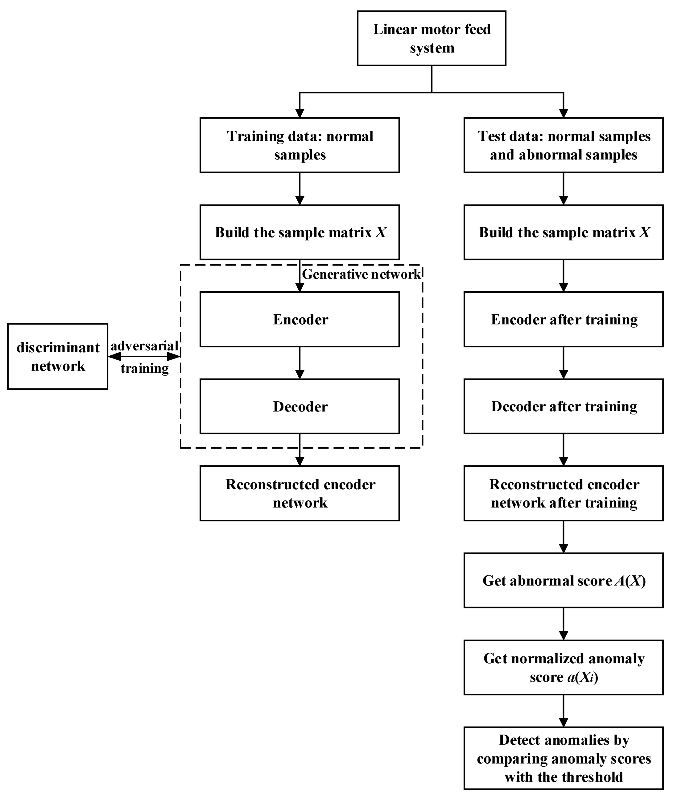
2.3. Anomaly Detection Process

The abnormal detection process of the linear motor feeding system proposed in this paper is displayed in Figure 6.

Training phase:

• STEP1: The sensor collects relevant time-series signals in real time, and a sample matrix $X$ is constructed for the collected normal samples.

  $$X=\left[\begin{array}{cccc}{x}_{11}& x_{12}& \cdots & x_{1n}\\ x_{21}& x_{22}& \cdots & x_{2n}\\ ⋮& ⋮& \ddots & ⋮\\ x_{m1}& x_{m2}& \cdots & x_{\mathit{mn}}\end{array}\right]$$

  (18)

  where $m$ is the number of samples in a sequence, and $n$ is the number of sensors.
• STEP2: The normal-sample matrix $X$ is inputted into the encoder $G_E\left(x\right)$, then the LSTM network extracts the time-series features, later the latent feature vector $Z$ is gained through three-layer fully connected layers, and lastly the reconstructed data $\hat{X}$ is obtained through the decoder $G_D\left(Z\right)$.
• STEP3: The discriminant network $D(x,\hat{x})$ discriminates the normal samples $X$ and the reconstructed data samples $\hat{X}$, and continuously narrows the gap between the two during the confrontational training process.
• STEP4: The reconstructed data $\hat{X}$ is inputted into the reconstructed encoder $E\left(\hat{x}\right)$ network, and then the latent feature vector $\hat{Z}$ is attained.

Test phase:

• STEP1: After the model training, the normal and abnormal samples are used to construct the sample matrix $X$ for testing. At this time, the discriminant network is no longer used. In the testing stage, network model parameters are fixed and outputted by training stage. The potential feature vector $Z$ is obtained through $G_E\left(x\right)$, then the reconstructed data $\hat{X}$ is gained through $G_D\left(Z\right)$, and finally, the potential feature vector of the reconstructed data $\hat{Z}$ is garnered through $E\left(\hat{x}\right)$.
• STEP2: The anomaly score $A\left(X\right)$ of the input sample $X$ is computed according to the loss functions $L_{\mathit{con}}$ and $L_{\mathit{enc}}$. The final anomaly score ${a(X}_i)$ is obtained by normalizing $A\left(X\right)$.
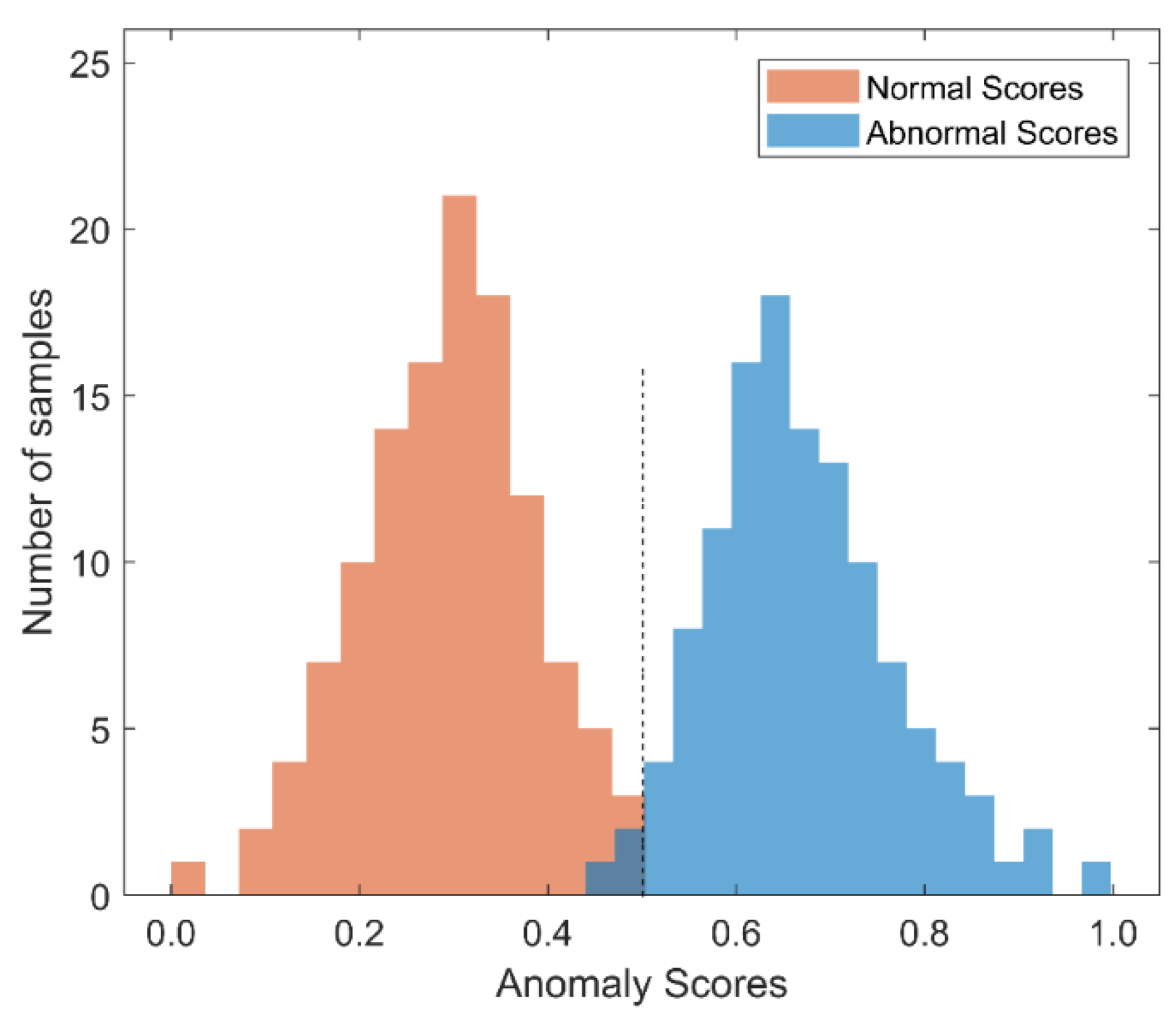
• STEP3: It is determined whether the input sample is abnormal or not according to the relationship between the abnormal score ${a(X}_i)$ and a certain threshold $\phi$. If ${a(X}_i)>\phi$, the input sample will be classified as an abnormal sample; otherwise it is a normal sample.

3. Experimental Setup and Feature Extraction

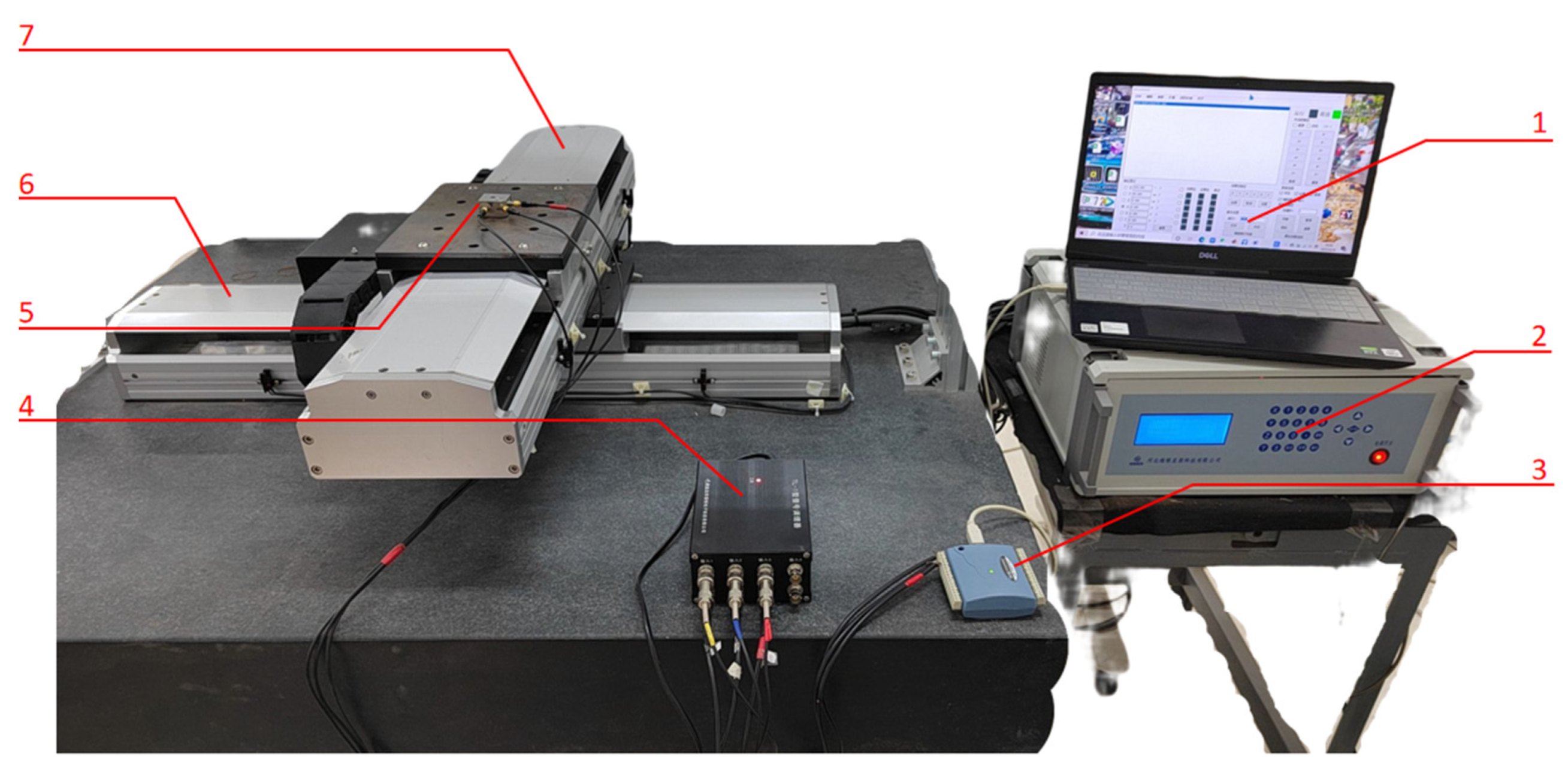
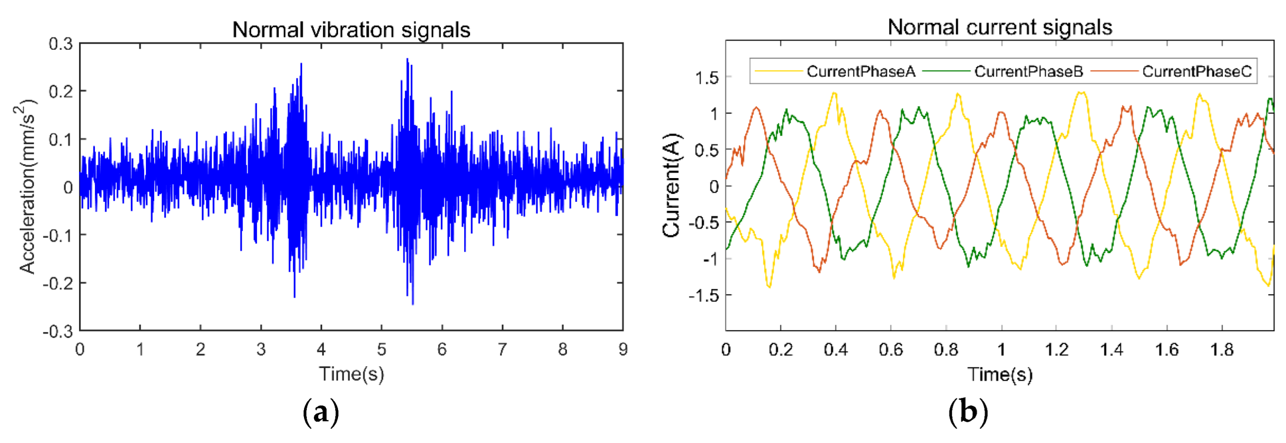
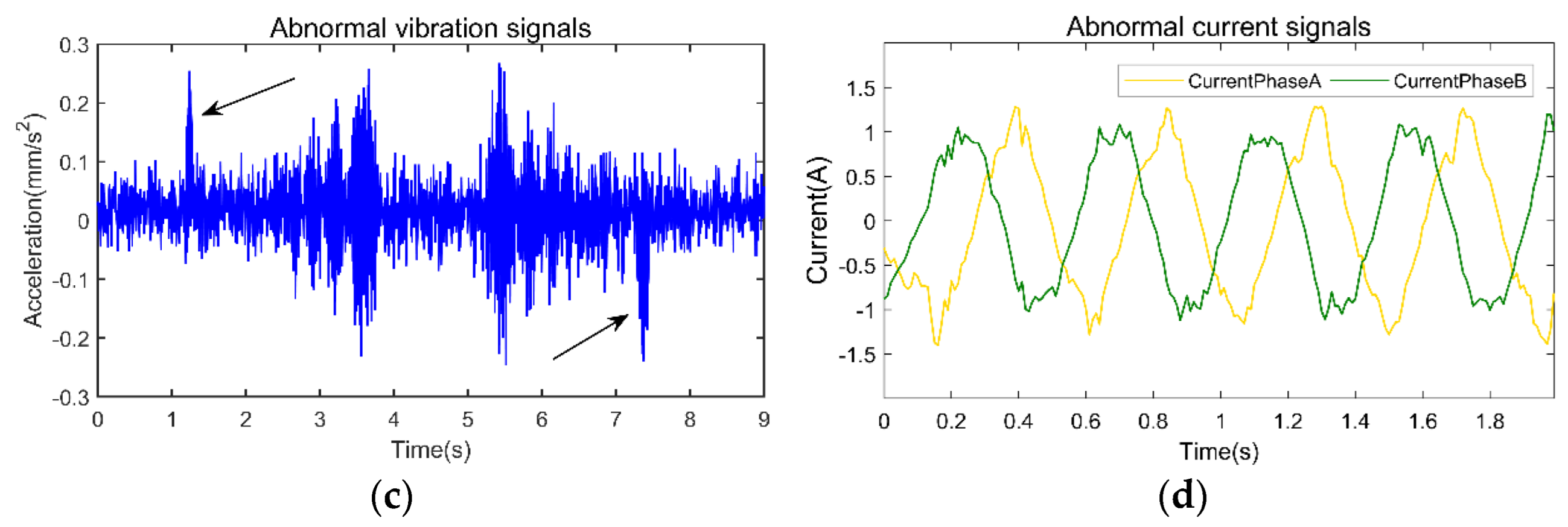
3.1. Construction of Experimental Platform and Data Collection

In order to verify the validity of the proposed method, an experimental platform for the linear motor feeding system is built, as presented in Figure 7 and

Table 2. Numbers and names of acquisition devices.

Number	Equipment Name
1	Computer processing center
2	Linear motor feeding system controller
3	Data acquisition card
4	Signal conditioner
5	Accelerometer
6	X-axis feeding system
7	Y-axis feeding system

. The platform consists of an X-Y two-axis linkage linear motor feeding system, a YD623 tri-axial accelerometer, a TL-1 signal conditioner, a USB-1608FS data acquisition card, a linear motor feeding system controller, and a computer processing center. The changeable working conditions of the experimental platform include feed speed, displacement and load, etc. The vibration signals in three directions and three-phase current signals are collected by setting different working conditions.

In order to obtain the vibration signals and current signals of the linear motor feeding system, the YD623 tri-axial accelerometer is fixed directly above the linear motor feeding system, and the vibration signals are collected by the USB-1608FS data acquisition card. The current sensor is located inside the system and connected to the computer via the appropriate data line. The current signals are measured by the software Composer. In this experiment, the sampling frequency is set to 50 kHz, and the sampling interval is 1 min. During the experiment, vibration signals in three directions are collected, and only the signals in the vertical direction are used in the data processing. The vibration signals of 2029 sampling points in the vertical direction are collected each time, and a total of 1,623,200 data points are collected in 800 groups. The three-phase current signals of 1533 sampling points are collected each time, and a total of 1,226,400 data points are collected in 800 groups.

During the experiment, vibration signals collected each time are stored in CSV files, and current signals are stored in MAT files. According to experimental conditions, each CSV file and MAT file are stored in corresponding folders, respectively.

3.2. Design of Experimental Working Conditions and Description of Data Samples

In order to obtain comprehensive and diverse experimental samples, the vibration signals and current signals of the linear motor feeding system under different operation commands are collected in this experiment. The collected data is divided into 16 categories according to the execution command parameters, and each category contains several time-acceleration sequence data and time-current data. The experimental working conditions for collecting the vibration and current signals in this experiment are shown in

Table 3. Experimental working condition settings.

Number	Load (kg)	X/Y Axis	Displacement Interval (mm)	Speed (mm/s)
1	No load	X axis	60, 180, 300, 420	60
2	No load	X axis	60, 180, 300, 420	80
3	No load	X axis	60, 180, 300, 420	100
4	No load	X axis	60, 180, 300, 420	120
5	No load	Y axis	60, 180, 300, 420	60
6	No load	Y axis	60, 180, 300, 420	80
7	No load	Y axis	60, 180, 300, 420	100
8	No load	Y axis	60, 180, 300, 420	120
9	No load	X-Y axis linkage	60, 180, 300, 420	60
10	No load	X-Y axis linkage	60, 180, 300, 420	80
11	No load	X-Y axis linkage	60, 180, 300, 420	100
12	No load	X-Y axis linkage	60, 180, 300, 420	120
13	Load 10 kg	X axis	60, 180, 300, 420	60
14	Load 10 kg	X axis	60, 180, 300, 420	80
15	Load 10 kg	X axis	60, 180, 300, 420	100
16	Load 10 kg	X axis	60, 180, 300, 420	120
17	Load 10 kg	Y axis	60, 180, 300, 420	60
18	Load 10 kg	Y axis	60, 180, 300, 420	80
19	Load 10 kg	Y axis	60, 180, 300, 420	100
20	Load 10 kg	Y axis	60, 180, 300, 420	120
21	Load 10 kg	X-Y axis linkage	60, 180, 300, 420	60
22	Load 10 kg	X-Y axis linkage	60, 180, 300, 420	80
23	Load 10 kg	X-Y axis linkage	60, 180, 300, 420	100
24	Load 10 kg	X-Y axis linkage	60, 180, 300, 420	120

. Figure 8a,b shows the vertical vibration signals and three-phase current signals which are collected in working condition 5 under a displacement interval of How 420 mm.

In this experiment, 800 samples of each of the vibration signal and current signal are collected. The dataset is divided into a 70% training set and 30% test set [45,46]. There are 560 samples in the training set, all of which are normal samples. The number of samples in the test set is 240, which are divided into two parts equally. Part of them are directly used as a normal sample for testing, and the other part are replaced with an abnormal sample. However, the life cycle of the linear motor feeding system is very long, and the probability of abnormality is small. Therefore, running to an abnormal state is an extremely time-consuming experiment in order to perform abnormal testing to obtain abnormal data. To overcome this difficulty, we introduce abnormal samples containing random amplitude shock noise in random positions of vibration signals. The abnormal samples of the vibration signal test set are shown in Figure 8c (the arrow position is the position where the noise is introduced). In order to obtain abnormal samples of the current signals, we collected the current signals of the missing phase. The abnormal samples of the current signals test set are shown in Figure 8d.

3.3. Experimental Environment and Model Parameters

This paper adopts PyTorch, a deep learning open-source framework, to construct the neural network model, complete the training, and test the model. PyTorch is widely used in computer vision, natural language processing and other fields.

The hardware environment of the computing deviceincludes a 4-core CPU Intel Xeon E3-123lv3, with a clock speed of 3.4 GHz; the GPU is AMD Radeon VII, with a memory capacity of 16 GB, and a memory speed of 4 Gbps and 3840 cores.

The Adam optimization algorithm is used in the training process, and the first-order moment weight β₁ = 0.6, while the second-order moment weight β₂ = 0.999. Since the GPU used in this experiment has enough video memory, the batch size used is 128, which can speed up the operation speed and convergence speed, and reduce the parameter jitter during training. Other model parameters are shown in

Table 4. The parameters of the model.

Parameters	${\mathit{\omega }}_{\mathit{adv}}$	${\mathit{\omega }}_{\mathit{con}}$	${\mathit{\omega }}_{\mathit{enc}}$	$\mathit{\lambda }$	Learning Rate
Value	1	1	0.5	0.8	0.0001

.

3.4. Signal Feature Extraction

In order to achieve a better abnormality detection effect of the linear motor feeding system, the extracted features must be appropriately selected. There is a lot of high noise and redundant information in the original data collected by sensors, which causes the dimension problem. The method based on deep learning can solve the above issues very well. An LSTM network is used to extract three effective time domain features from the original vibration and current signals, namely, standard deviation, skewness and kurtosis. After repeated experiments, it is found that these three statistical features are susceptible to the abnormal changes in the vibration signals and current signals. Two hundred and forty feature datasets are extracted from the vibration and current signal test sets, respectively. Figure 9 shows three time-domain feature scatter plots of vibration signals and current signals in working condition 5 under a displacement interval of 420 mm. The results show that both the sample features of the vibration signals and the current signals can achieve good classification. However, the sample feature aggregation effect of the current signals is better than that of the vibration signal, and the classification effect is more pronounced.

4. Analysis of Experimental Results

To verify the performance of the proposed method, the performances under the following three different input conditions are compared.

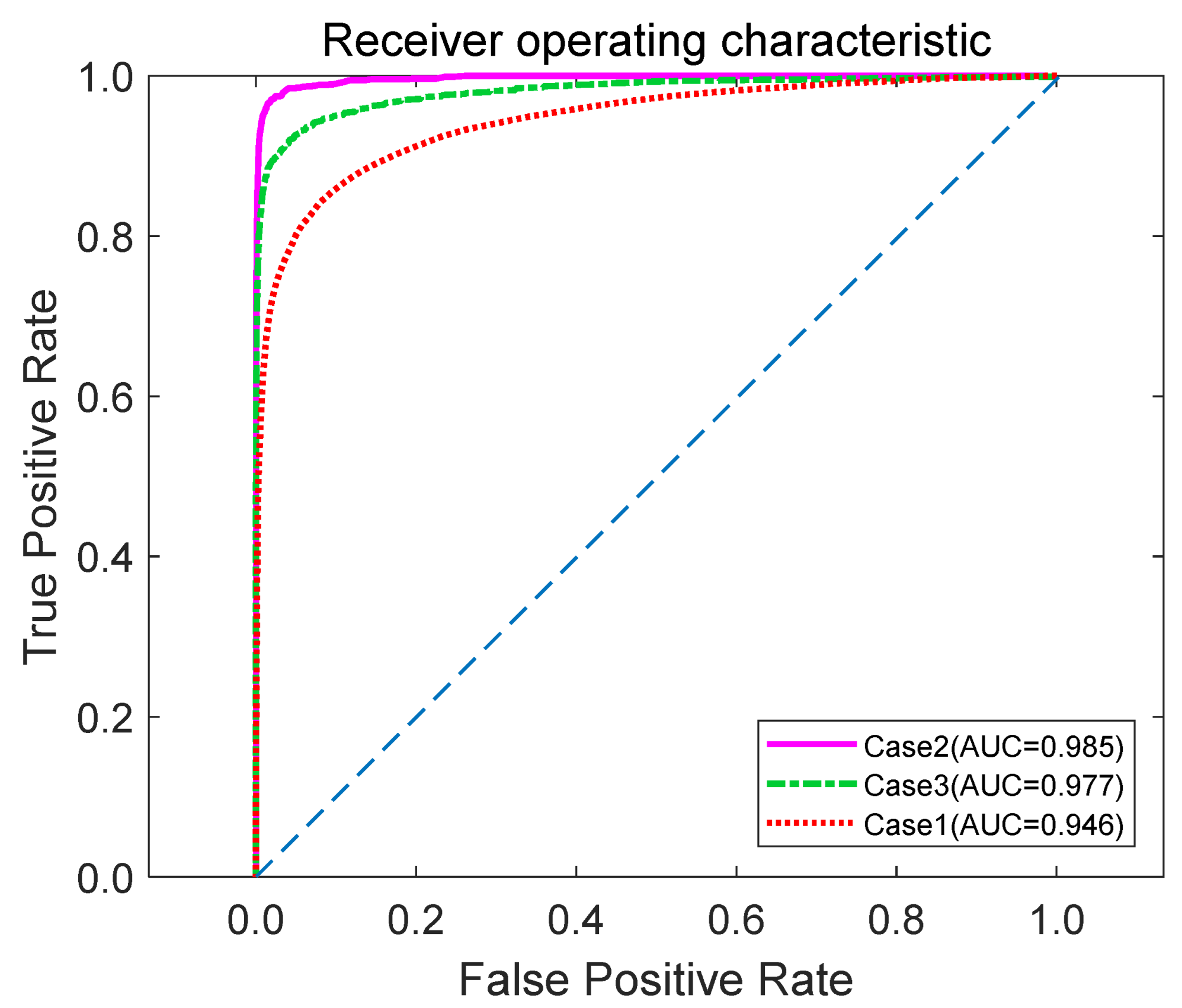
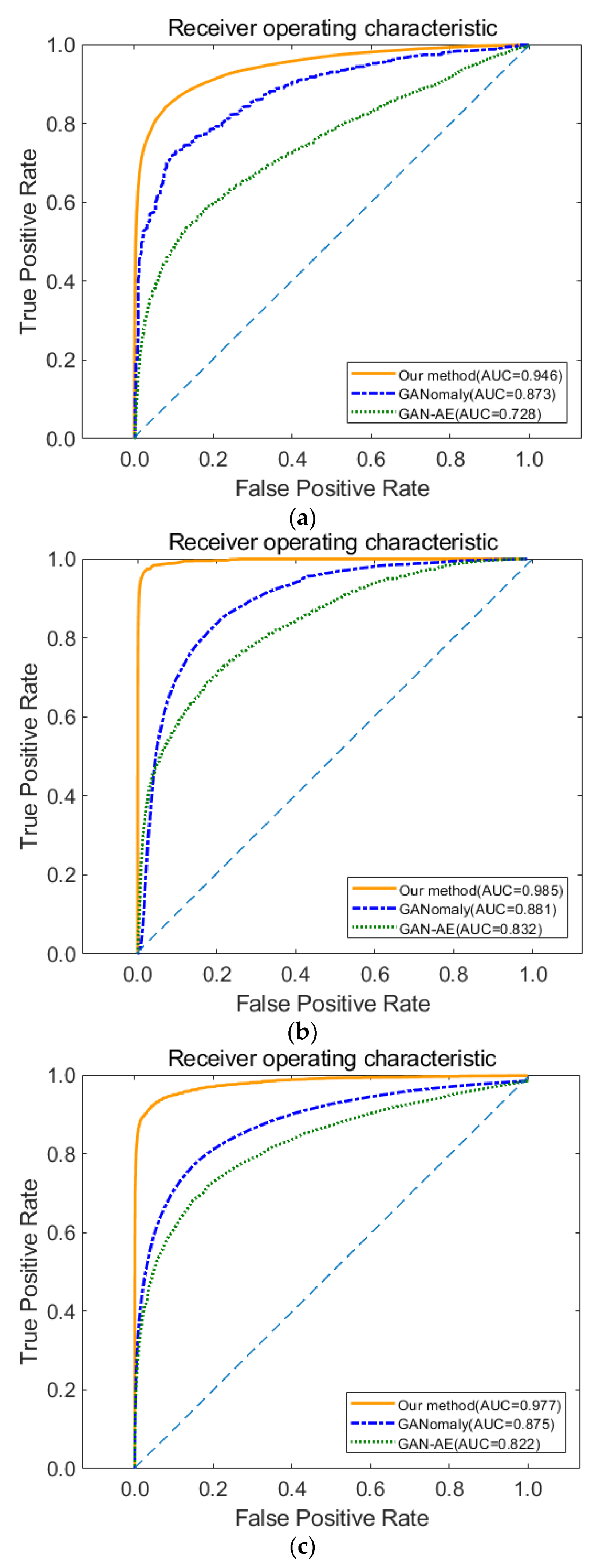
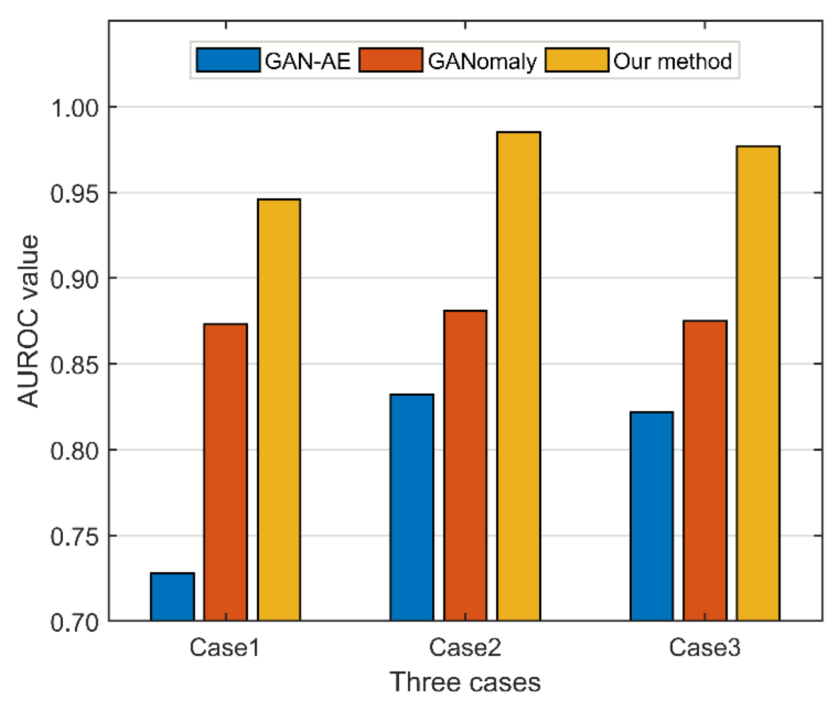
• Case1: Vibration data sample;
• Case2: Current data sample;
• Case3: Vibration and Current Composite Data Sample.

Figure 10 exhibits the ROC curves of our method under different input conditions. It is obvious that the AUROC indicators under the three input conditions are above 90%, especially in Case2, which reaches 98.5%, the maximum value, compared to 94.6% and 97.7% in the other two cases, an improvement of 3.9% and 0.8%, respectively. In order to further certify the accuracy of the comparison, we introduce the AUPRC indicator for comparison. The experimental results are shown in

Table 5. Experimental results of our method under three input conditions.

Case	AUROC	AUPRC
Case 1	0.946	0.948
Case 2	0.985	0.982
Case 3	0.977	0.969

, and the change trends of the two indicators are generally consistent. For the AUPRC, it reaches 98.2% in Case2, compared to 94.8% and 96.9% in the other two cases, an improvement of 3.4% and 1.3%, respectively. Figure 11 is the histogram of normal and abnormal scores when the method in this paper uses current data samples alone. It can be seen that our model can distinguish normal and abnormal classes well. To further compare the accuracy of the models under the three input conditions, we calculated the precision score, recall score and F₁ score under the three input conditions. As shown in Figure 11, the dividing line between normal and abnormal scores is about 0.5, that is, the threshold $\phi$ = 0.5. Therefore, our model distinguishes samples with scores less than 0.5 as normal samples and otherwise abnormal. We set the threshold at 0.44, when the recall rate of abnormal samples is 1, to compare the scores under three input conditions. As can be seen from

Table 6. Evaluation results of our method under three input conditions (the threshold is set to 0.44).

Case	Precision	Recall	F1
Case 1	0.921	0.953	0.937
Case 2	0.965	1.000	0.982
Case 3	0.943	0.984	0.963

, the proposed method achieves the maximum values on the three metrics of Case2, which are 96.5%, 100%, and 98.2%, respectively.

The aforementioned experimental results reflect that the proposed method is a valid and feasible anomaly detection method for time-series data, and remarkable results are achieved under the above three input conditions. That is, the GANomaly-LSTM method has excellent effects on the identification of current phase missing and abnormal vibration of the linear motor feeding system.

To further test and verify the performance of the proposed method, we compared the performances of the three methods under three input conditions. The other two methods are GANomaly and GAN-AE. In order to ensure the effectiveness of the method comparison, the parameter settings of these two methods are exactly the same as the proposed method. The reasons for choosing these two methods to compare with the proposed method are: (1) The network structures of these two methods are similar to that of the proposed method, which is based on the extension of the GAN and adopts the structure of encoding-decoding-encoding; (2) These two methods and the proposed method only use normal samples during training, and use normal and abnormal samples during testing; (3) All three detect anomalies by the difference between the latent features after two encodings. Therefore, it is essential to choose these two methods to compare with our method.

During training, Case1 uses 560 normal samples of vibration signals, Case2 uses 560 normal samples of current signals, and Case3 uses the training set of the first two. In the testing process, Case1 uses the vibration signals of 120 normal samples and 120 abnormal samples, Case2 uses the current signals of 120 normal samples and 120 abnormal samples, and Case3 uses the test sets of the former two at the same time. Figure 12 shows the ROC curves of the three methods under three input conditions. It can be seen that the AUROC metric of the proposed method under the three input conditions is significantly higher than the other two methods. It is shown in

Table 7. AUROC metrics for three methods under three input conditions.

AUROC	Case1	Case2	Case3
GAN-AE	0.728	0.832	0.822
GANomaly	0.873	0.881	0.875
Our method	0.946	0.985	0.977

that our method achieves the optimal accuracy in the AUROC indicator under the three input conditions, and achieves good performance in the task of abnormal detection of the running state of the linear motor feeding system, showing tremendous advantages. Specifically, the AUROC indicators of GANomaly are 87.3%, 88.1% and 87.5%, respectively, while GAN-AE performs poorly, at only 72.8%, 83.2% and 82.2%, respectively. That is, the AUROC metrics of the proposed method are 94.6%, 98.5% and 97.7%, which are 7.3%, 10.4% and 10.2% higher than GANomaly. Figure 13 compares the experimental results of the three methods under three input conditions in the form of histograms. It can be distinctly shown that all three methods achieve the best results under the condition of Case2. Under Case2, we further compare the average accuracy and detection time of the three methods, shown in

Table 8. Comparison of the average accuracy and detection time of the three methods when using current data samples alone.

Case	Average Accuracy	Detection Time (ms)
GAN-AE	0.825	418
GANomaly	0.864	357
Our method	0.980	134

, the average accuracies of the proposed method, GANomaly, and GAN-AE achieves 98%, 86.4% and 82.5%; the detection times are 134 ms, 357 ms and 418 ms, respectively. Our method has an average accuracy improvement of 11.6% and 15.5%, and a detection time shortened by 223 ms and 284 ms, respectively, compared with the classical two methods.

The above experimental results demonstrate that the proposed method achieves a more pronounced improvement in detection accuracy, a shorter detection time and more significant results. In general, the proposed method is highly effective for abnormal detection of the running state of linear motor feeding systems, meeting the application requirements in industrial production. This method solves the task of anomaly detection in the absence of abnormal sample training, and has profound significance for improving industrial production efficiency and equipment predictive maintenance.

5. Conclusions

This paper proposes an anomaly detection method based on GANomaly-LSTM for the running status of the linear motor feeding system. This method solves the problem of anomaly detection in the linear motor feeding systems when there is no abnormal sample and the sample timing is significant. This method compares the anomaly detection performance of the model under three input conditions (vibration data sample, current data sample, vibration and current combination data sample). The AUROC indexes are 94.6%, 98.5% and 97.7%, and the F1 scores are 93.7%, 98.2% and 96.3%, respectively. The consequences show that the proposed method has favorable detection performances. In addition, compared with GANomaly and GAN-AE, the proposed method improved the average AUROC indicator by 9.3% and 17.5%, respectively, thus greatly enhancing the anomaly detection accuracy. In sum, the GANomaly-LSTM method has excellent effects on the identification of the current phase missing and abnormal vibration of the linear motor feeding system. Due to the variety of abnormal conditions in the linear motor feeding system and varying types of abnormal samples, the limitation of our method lies in the need for retraining and retesting different types of samples. In addition, the applicability of the method for other anomalies such as current single phase short circuit and voltage anomalies needs to be further investigated. For future works, we expect to investigate more data types such as torque and power along with the current and vibration signals of the linear motor feeding system, and to compare the effects of different sample sizes on detection accuracy to achieve more efficient and comprehensive anomaly detection. In future research, we hope to realize further fault location based on anomaly detection to achieve more accurate predictive maintenance.

References

1. Altintas, Y.; Verl, A.; Brecher, C.; Uriarte, L.; Pritschow, G. Machine tool feed drives. CIRP Ann. Manuf. Technol. 2010, 60, 779–796. [Google Scholar] [CrossRef]
2. Wang, B.; Mao, Z. Outlier detection based on Gaussian process with application to industrial processes. Appl. Soft. Comput. 2019, 76, 505–516. [Google Scholar] [CrossRef]
3. Jin, X.; Sun, Y.; Que, Z.; Wang, Y.; Zhou, X. Anomaly detection and fault prognosis for bearings. IEEE Trans. Instrum. Meas. 2016, 65, 2046–2054. [Google Scholar] [CrossRef]
4. Liu, J.; Liu, L.; Du, J.; Sang, J. TLE outlier detection based on expectation maximization algorithm. Adv. Space Res. 2021, 68, 2695–2712. [Google Scholar] [CrossRef]
5. Su, J.; Dong, Y.; Yan, M.; Qian, J.; Xin, Y. Research progress of anomaly detection for complex networks. Control Decis. 2021, 36, 1293–1310. [Google Scholar]
6. Li, Z.; Jin, X.; Zhuang, C.; Sun, Z. A Survey of Graph-Oriented Anomaly Detection Research. J. Softw. 2021, 32, 167–193. [Google Scholar] [CrossRef]
7. Zhang, S.; Li, X.; Zong, M.; Zhu, X.; Wang, R. Efficient kNN Classification with Different Number of Nearest Neighbors. IEEE Trans. Neural Netw. Learn. Syst. 2018, 29, 1774–1785. [Google Scholar] [CrossRef] [PubMed]
8. Li, J.; Izakian, H.; Pedrycz, W.; Jamal, I. Clustering-based anomaly detection in multivariate time series data. Appl. Soft. Comput. 2021, 100, 106919. [Google Scholar] [CrossRef]
9. Li, T.; Comer, M.L.; Delp, E.J.; Desai, S.R.; Mathieson, J.L.; Foster, R.H.; Chan, M.W. Anomaly Scoring for Prediction-Based Anomaly Detection in Time Series. In Proceedings of the 2020 IEEE Aerospace Conference, Big Sky, MT, USA, 7–14 March 2020; pp. 1–7. [Google Scholar]
10. Zhou, Y.; Ren, H.; Li, Z.; Wu, N.; AI-Ahmari, A.M. Anomaly detection via a combination model in time series data. Appl. Intell. 2021, 51, 4874–4887. [Google Scholar] [CrossRef]
11. Abdulghafoor, S.A.; Mohamed, L.A. A local density-based outlier detection method for high dimension data. Int. J. Nonlinear Anal. Appl. 2022, 13, 1683–1699. [Google Scholar]
12. Jin, W.; Tung, A.K.H.; Han, J.; Wang, W. Ranking Outliers using Symmetric Neighborhood Relationship. In Advances in Knowledge Discovery and Data Mining; Ng, W.K., Kitsuregawa, M., Li, J., Chang, K., Eds.; Lecture Notes in Computer Science; Springer International Publishing: Berlin/Heidelberg, Germany, 2006; Volume 3918, pp. 577–593. ISBN 978-3-540-33206-0. [Google Scholar]
13. Zhao, R.; Yan, R.; Chen, Z. Deep learning and its applications to machine health monitoring. Mech. Syst. Signal Proc. 2019, 115, 213–237. [Google Scholar] [CrossRef]
14. Hoang, D.T.; Kang, H.J. Rolling element bearing fault diagnosis using convolutional neural network and vibration image. Cogn. Syst. Res. 2019, 53, 42–50. [Google Scholar] [CrossRef]
15. Shao, H.; Ding, Z.; Cheng, J.; Jiang, H. Intelligent fault diagnosis among different rotating machines using novel stacked transfer auto-encoder optimized by PSO. ISA Trans. 2020, 105, 308–319. [Google Scholar]
16. Jiang, G.; Zhao, J.; Jia, C.; He, Q.; Xie, P.; Meng, Z. Intelligent fault diagnosis of gearbox based on vibration and current signals: A multimodal deep learning approach. In Proceedings of the 2019 Prognostics and System Health Management Conference, Qingdao, China, 25–27 October 2019; pp. 1–6. [Google Scholar]
17. Goodfellow, I.J.; Pouget-Abadie, J.; Mirza, M.; Xu, B.; Warde-Farley, D.; Ozair, S.; Courville, A.; Bengio, Y. Generative adversarial networks. Available online: https://arxiv.org/abs/1406.2661 (accessed on 20 June 2022).
18. Xia, X.; Pan, X.; Li, N.; He, X.; Ma, L.; Zhang, X.; Ding, N. GAN-based Anomaly Detection: A Review. Neurocomputing 2022, 493, 497–535. [Google Scholar] [CrossRef]
19. Zenati, H.; Foo, C.S.; Lecouat, B.; Manek, G.; Chandrasekhar, V.R. Efficient Ganbased Anomaly Detection. Available online: https://arxiv.org/abs/1802.06222 (accessed on 20 June 2022).
20. Radford, A.; Metz, L.; Chintala, S. Unsupervised representation learning with deep convolutional generative adversarial networks. Available online: https://arxiv.org/abs/1511.06434 (accessed on 20 June 2022).
21. Schlegl, T.; Seeböck, P.; Waldstein, S.M.; Schmidt-Erfurth, U.; Langs, G. Unsupervised anomaly detection with generative adversarial networks to guide marker discovery. In Information Processing in Medical Imaging; Niethammer, M., Styner, M., Aylward, S., Zhu, H., Ogue, L., Yap, P., Shen, D., Eds.; Lecture Notes in Computer Science; Springer International Publishing: Cham, Switzerland, 2017; Volume 10265, pp. 146–157. ISBN 978-3-319-59049-3. [Google Scholar]
22. Wang, Z.; Wang, J.; Wang, Y. An intelligent diagnosis scheme based on generative adversarial learning deep neural networks and its application to planetary gearbox fault pattern recognition. Neurocomputing 2018, 310, 213–222. [Google Scholar] [CrossRef]
23. Mao, W.; Liu, Y.; Ding, L.; Yuan, L. Imbalanced Fault Diagnosis of Rolling Bearing Based on Generative Adversarial Network: A Comparative Study. IEEE Access 2019, 7, 9515–9530. [Google Scholar] [CrossRef]
24. Gao, X.; Deng, F.; Yue, X. Data augmentation in fault diagnosis based on the Wasserstein generative adversarial network with gradient penalty. Neurocomputing 2020, 396, 487–494. [Google Scholar] [CrossRef]
25. Akçay, S.; Atapour-Abarghouei, A.; Breckon, T.P. GANomaly: Semi-supervised anomaly detection via adversarial training. In Computer Vision-ACCV 2018; Jawahar, C., Li, H., Mori, G., Schindler, K., Eds.; Lecture Notes in Computer Science; Springer International Publishing: Cham, Switzerland, 2019; Volume 11363, pp. 622–637. ISBN 978-3-030-20892-9. [Google Scholar]
26. Akçay, S.; Atapour-Abarghouei, A.; Breckon, T.P. Skip-GANomaly: Skip connected and adversarially trained encoder-decoder anomaly detection. In Proceedings of the 2019 International Joint Conference on Neural Networks (IJCNN), Budapest, Hungary, 14–19 July 2019; pp. 1–8. [Google Scholar]
27. Luo, Z.; Zuo, R.; Xiong, Y.; Wang, X. Detection of geochemical anomalies related to mineralization using the GANomaly network. Appl. Geochem. 2021, 131, 105043. [Google Scholar] [CrossRef]
28. Liu, G.; Niu, Y.; Zhao, W.; Duan, Y.; Shu, J. Data anomaly detection for structural health monitoring using a combination network of GANomaly and CNN. Smart. Struct. Syst. 2022, 29, 53–62. [Google Scholar]
29. Hong, Z.; Yang, Z.; Yang, C.; Liao, S.; Sun, Y.; Xing, Y. Triple-GAN with Fixed Memory Step Gradient Descent Method and Xwish Activation Function. In Proceedings of the 2020 39th Chinese Control Conference (CCC), Shenyang, China, 27–29 July 2020; pp. 3188–3193. [Google Scholar]
30. Duan, S.; Chen, Z.; Wu, Q.M.J.; Cai, L.; Lu, D. Multi-scale gradients self-attention residual learning for face photo-sketch transformation. IEEE Trans. Inf. Forensic Secur. 2020, 16, 1218–1230. [Google Scholar] [CrossRef]
31. Lindemann, B.; Maschler, B.; Sahlab, N.; Weyrich, M. A survey on anomaly detection for technical systems using LSTM networks. Comput. Ind. 2021, 131, 103498. [Google Scholar] [CrossRef]
32. Li, Z.; Li, J.; Wang, Y.; Wang, K. A deep learning approach for anomaly detection based on SAE and LSTM in mechanical equipment. Int. J. Adv. Manuf. Technol. 2019, 103, 499–510. [Google Scholar] [CrossRef]
33. Chen, H.; Liu, H.; Chu, X.; Liu, Q.; Xue, D. Anomaly detection and critical SCADA parameters identification for wind turbines based on LSTM-AE neural network. Renew. Energy 2021, 172, 829–840. [Google Scholar] [CrossRef]
34. Vos, K.; Peng, Z.; Jenkins, C.; Shahriar, M.R.; Borghesani, P.; Wang, W. Vibration-based anomaly detection using LSTM/SVM approaches. Mech. Syst. Signal Proc. 2022, 169, 108752. [Google Scholar] [CrossRef]
35. Ou, X.; Wen, G.; Huang, X.; Su, Y.; Chen, X.; Lin, H. A deep sequence multi-distribution adversarial model for bearing abnormal condition detection. Measurement 2021, 182, 109529. [Google Scholar] [CrossRef]
36. Bai, M.; Liu, J.; Ma, Y.; Zhao, X.; Long, Z.; Yu, D. Long Short-Term Memory Network-Based Normal Pattern Group for Fault Detection of Three-Shaft Marine Gas Turbine. Energies 2021, 14, 13. [Google Scholar] [CrossRef]
37. Kong, F.; Li, J.; Jiang, B.; Wang, H.; Song, H. Integrated generative model for industrial anomaly detection via bi-directional LSTM and attention mechanism. IEEE Trans. Ind. Inform. 2021. [Google Scholar] [CrossRef]
38. Yang, H.; Wang, Z.; Zhang, T.; Du, F. A review on vibration analysis and control of machine tool feed drive systems. Int. J. Adv. Manuf. Technol. 2020, 107, 1–23. [Google Scholar] [CrossRef]
39. Yan, K. Chiller fault detection and diagnosis with anomaly detective generative adversarial network. Build. Environ. 2021, 201, 107982. [Google Scholar] [CrossRef]
40. Du, J.; Guo, L.; Song, L.; Liang, H.; Chen, T. Anomaly detection of aerospace facilities using GANomaly. In Proceedings of the 2020 5th International Conference on Multimedia Systems and Signal Processing, Wuhan, China, 8–10 May 2020; pp. 40–44. [Google Scholar]
41. Wang, F.; Liu, X.; Deng, G.; Yu, X.; Li, H.; Han, Q. Remaining life prediction method for rolling bearing based on the long short-term memory network. Neural Process. Lett. 2019, 50, 2437–2454. [Google Scholar] [CrossRef]
42. Huang, R.; Wei, C.; Wang, B.; Yang, J.; Xu, X.; Wu, S.; Huang, S. Well performance prediction based on Long Short-Term Memory (LSTM) neural network. J. Pet. Sci. Eng. 2022, 208, 109686. [Google Scholar] [CrossRef]
43. Ruder, S. An Overview of Gradient Descent Optimization Algorithms. Available online: https://arxiv.org/abs/1609.04747 (accessed on 30 July 2022).
44. Kingma, D.P.; Ba, J. Adam: A method for Stochastic Optimization. Available online: https://arxiv.org/abs/1412.6980 (accessed on 30 July 2022).
45. Chen, Z.; Gryllias, K.; Li, W. Intelligent Fault Diagnosis for Rotary Machinery Using Transferable Convolutional Neural Network. IEEE Trans. Ind. Inform. 2020, 16, 339–349. [Google Scholar] [CrossRef]
46. Ravikumar, K.N.; Yadav, A.; Kumar, H.; Gangadharan, K.V.; Narasimhadhan, A.V. Gearbox fault diagnosis based on Multi-Scale deep residual learning and stacked LSTM model. Measurement 2021, 186, 110099. [Google Scholar] [CrossRef]
Figure 1. Network structure of GANomaly.
Energies 15 05671 g001
Figure 2. Network structure of LSTM: (a) Unit structure of LSTM; (b) Recurrent structure of LSTM.
Energies 15 05671 g002aEnergies 15 05671 g002b
Figure 3. Three activation functions: (a) Sigmoid; (b) Tanh; (c) ReLU.
Energies 15 05671 g003
Figure 4. The network structure of GANomaly-LSTM.
Energies 15 05671 g004
Figure 5. Network structure of encoder.
Energies 15 05671 g005
Figure 6. Anomaly detection workflow.
Energies 15 05671 g006
Figure 7. X-Y two-axis linkage linear motor feeding system experimental platform.
Energies 15 05671 g007
Figure 8. Normal and abnormal time domain vibration and current signals in working condition 5 under (displacement interval 420 mm): (a) Normal vibration signals; (b) Normal current signals; (c) Abnormal vibration signals (the arrow position is the position where the noise is introduced); (d) Abnormal current signals.
Energies 15 05671 g008aEnergies 15 05671 g008b
Figure 9. The distribution scatters diagram of the three-time domain features in working condition 5 under displacement interval 420 mm: (a) Feature distribution of vibration signals; (b) Feature distribution of the current signals.
Energies 15 05671 g009
Figure 10. ROC curves of our method under different input conditions.
Energies 15 05671 g010
Figure 11. Histograms of normal and abnormal scores for samples of current data tested with our method.
Energies 15 05671 g011
Figure 12. ROC curves of three methods under three input conditions: (a) Case1; (b) Case2; (c) Case3.
Energies 15 05671 g012
Figure 13. Histograms of experimental results for three methods under three input conditions.
Energies 15 05671 g013