An MILP-Based Distributed Energy Management for Coordination of Networked Microgrids

Abstract

An MILP-based distributed energy management for the coordination of networked microgrids is proposed in this paper. Multiple microgrids and the utility grid are coordinated through iteratively adjusted price signals. Based on the price signals received, the microgrid controllers (MCs) and distribution management system (DMS) update their schedules separately. Then, the price signals are updated according to the generation–load mismatch and distributed to MCs and DMS for the next iteration. The iteration continues until the generation–load mismatch is small enough, i.e., the generation and load are balanced under agreed price signals. Through the proposed distributed energy management, various microgrids and the utility grid with different economic, resilient, emission and socio-economic objectives are coordinated with generation–load balance guaranteed and the microgrid customers’ privacy preserved. In particular, a piecewise linearization technique is employed to approximate the augmented Lagrange term in the alternating direction method of multipliers (ADMM) algorithm. Thus, the subproblems are transformed into mixed integer linear programming (MILP) problems and efficiently solved by open-source MILP solvers, which would accelerate the adoption and deployment of microgrids and promote clean energy. The proposed MILP-based distributed energy management is demonstrated through various case studies on a networked microgrids test system with three microgrids.

1. Introduction

A microgrid is a local energy system with locally installed distributed energy resources (DERs), such as distributed generators (DGs) and energy storage systems (ESSs), which provide low-cost and clean energy to local consumers. Generally, a microgrid interconnects with a distribution grid at a Point of Common Coupling (PCC). When grid-connected, a microgrid can make profit through arbitrage, utilizing the temporal price discrepancies of the utility grid. In addition, a microgrid could facilitate the secure and efficient operation of the utility grid by providing operational supports in many aspects, e.g., frequency and voltage regulation, virtual inertia, etc. [1,2,3,4]. As a unique virtue, a microgrid could seamlessly transit from grid-connected to islanding operation and continue to supply its local customers independently [5,6]. Thus, microgrids could effectively enhance the resilience of power supply [7]. With due consideration of these benefits, microgrids have been increasingly deployed all over the world [8].

While the advantages of a single microgrid for improving energy efficiency and enhancing resilience have been well-recognized, connecting multiple adjacent microgrids to form a distribution system with networked microgrids provides a more efficient and resilient alternative. During normal operation, these microgrids could exchange electricity for more efficient and economical operation; while under emergency scenarios, interconnecting individual microgrids could facilitate maximizing the overall system resilience through sharing capacities and flexibilities with each other. In addition, networked microgrids could be designed to protect not only the critical loads inside the microgrids but also neighboring loads as well. For these benefits, networked microgrids have attracted growing attention [9].

The coordinated energy management of networked microgrids is necessary for achieving both economic benefits and resiliency improvements. Generally, existing research work on the energy management of networked microgrids could be classified into two categories: centralized energy management and distributed energy management [10,11]. Centralized energy management systems are usually formulated as a two-level hierarchical framework. In the lower level, each microgrid schedules internal DERs and loads, while in the upper layer, multiple microgrids are coordinated through a centralized optimal power flow [12]. In [13], the dispatching strategy of networked microgrids in distribution grids is formulated as a bi-level optimization. A more general nested scheduling strategy with multiple levels was formulated for the energy management of networked microgrids in [14]. In [15], a three-phase unbalanced optimal power flow model is presented for networked microgrids coordination and solved by semidefinite programming (SDP). Considering uncertainties of renewable DERs and loads, a bi-level stochastic programming is put forward to schedule the energy and reserve of distribution grids in the presence of renewable-based microgrids and other autonomous players in [16]. A robust counterpart considering various uncertainties is proposed in [17,18]. A low-carbon economic dispatch model for multi-energy microgrids is proposed to effectively reduce the carbon emission while greatly decreasing the operation cost in [19].

Although these centralized methods are straightforward to formulate and have the potential to achieve global optimality, they may suffer from computational scalability and privacy issues. Distributed methods ensure coordination between individual microgrids with privacy, which addresses the scalability issue. Thus, distributed energy management is more popular than centralized energy management for networked microgrids coordination. The multi-agent system (MAS)-based game theoretical framework is a common distributed approach used for optimizing energy trading among networked microgrids [20]. In [21], a non-cooperative Stackelberg game is proposed for the Peer-to-Peer (P2P) energy trading among grid-connected networked microgrids. Another widely used distributed optimization method is dual decomposition, which is suitable to the situation in which the distribution grid and microgrids are owned by different entities, and these entities need to conduct negotiations among all entities based on their own objectives and policies [22,23,24]. Dual decomposition enables the autonomy and privacy of users and the parallel processing of individual microgrid energy management. However, the convergence of dual decomposition requires a strict convexity or finiteness, and its robustness is worse. For this reason, the alternating direction method of multipliers (ADMM), which adds an augmented Lagrange term to improve the convergence without convexity or finiteness assumptions, has gained more popularity than dual decomposition [25,26,27,28,29,30]. In [27,28,29], the original non-convex optimal power flow problem is equivalently transformed into a convex second-order cone programming problem, which could be efficiently solved by commercial solvers. In [31], a consensus algorithm is employed to reach a nodal price agreement among microgrids while complying with the energy balance constraint. Nevertheless, the marginal cost functions of microgrids are assumed to be known and linear, which is not always available in practice.

The existing literature on ADMM-based distributed energy management for coordination networked microgrids mostly decomposed the centralized optimization into parallel subproblems of microgrid controllers (MCs) and a distribution management system (DMS). Due to the added augmented Lagrange term, both subproblems are formulated as mixed integer quadratic programming (MIQP), which are solved by commercial MIQP solvers, such as CPLEX [32] or GUROBI [33]. To improve the efficiency and avoid the expensive license cost of commercial solvers, an MILP-based distributed energy management for the coordination of networked microgrids is proposed in this paper. To be specific, a piecewise linearization technique is employed to approximate the augmented Lagrange term in the ADMM algorithm. As a result, both subproblems are transformed into mixed integer linear programing (MILP), which could be efficiently solved by a free and open-source MILP solver, e.g., COIN Branch and Cut solver (CBC), without compromising the solution accuracy [34]. The solution of the proposed MILP-based distributed energy management coordinates various microgrids and the utility grid with generation–load balance guaranteed and microgrid customers’ privacy preserved.

For simplicity, the proposed MILP-based distributed energy management system is compared with existing distributed energy management systems for networked microgrids in

Table 1. Comparison of distributed energy management for networked microgrids.

Algorithms	Convergence for Convex Problem	Convergence for Non-Convex Problem	Optimization Model	References
Stackelberg Game	Yes	Mostly No	MILP/MIQP	[20,21]
Consensus Algorithm	Yes	No	MILP	[31]
Dual Decomposition	Mostly Yes	No	MILP	[22,23,24]
ADMM	Yes	Mostly Yes	MIQP	[25,26,27,28,29,30]
Proposed MILP-Based Approach	Yes	Mostly Yes	MILP	This Paper

. As can be seen, all these distributed energy management converge well for convex optimization problems except dual decomposition. However, only ADMM and the proposed MILP-based distributed energy management mostly converge with modest accuracy for non-convex optimization problems. Given the fact that ADMM introduced an augmented Lagrange term in the subproblems to drive the convergence, ADMM requires commercial MIQP solvers, such as CPLEX or GUROBI. The proposed MILP-based distributed energy management, by contrast, could be more efficiently solved than MIQP models. More importantly, the proposed MILP-based method could be solved by free and opensource MILP solvers, which facilitates the adoption and deployment of networked microgrids.

The main contributions are listed as follows:

• An MILP-based distributed energy management through approximating the augmented Lagrange term in ADMM with a piecewise linearization technique is proposed for the coordination of networked microgrids. Comparing with ADMM, the proposed MILP-based distributed energy management is more efficient. Unlike ADMM, the proposed MILP-based distributed energy management could be solved by open-source MILP solvers.
• The effectiveness and efficiency of the proposed MILP-based distributed energy management system are validated through comparing with the case study results of both centralized optimization and ADMM-based distributed energy management.

As to the structure of this paper, the microgrid components and networked microgrids are introduced in Section 2. Section 3 describes the centralized energy management for the coordination of networked microgrids. The ADMM-based and proposed MILP-based distributed energy management systems are presented in Section 4. In Section 5, the results of case studies are presented and analyzed. Finally, Section 6 concludes the paper.

2. Modeling

2.1. Microgrid

A microgrid generally includes locally installed DGs, ESSs and various loads. Normally, the operation of a microgrid is supervised by an MC, which monitors system states and sends dispatch orders to controllable components. There are two types of DGs in microgrids: dispatchable or undispatchable. Diesel generators, microturbines, fuel cells, etc., are dispatchable DGs, which are able to respond to the request of MCs and change its power output accordingly. On the contrary, wind turbines and PV are typical undispatchable DGs, whose power outputs are largely affected by the uncertain nature of the environmental condition and could not be controlled completely. In reality, the power outputs of these undispatchable DGs are forecasted with limited accuracy. The hour-ahead forecast error of the wind turbine output is around 10% [35]. The forecasting of PV output is more difficult because of the random cloud coverage and changing ambient temperature. Both could significantly affect the generation of PV [36]. To mitigate these uncertainties, ESSs are generally installed on-site. For simplicity, the wind and PV power forecast errors have been neglected in this work.

2.2. Networked Microgrids

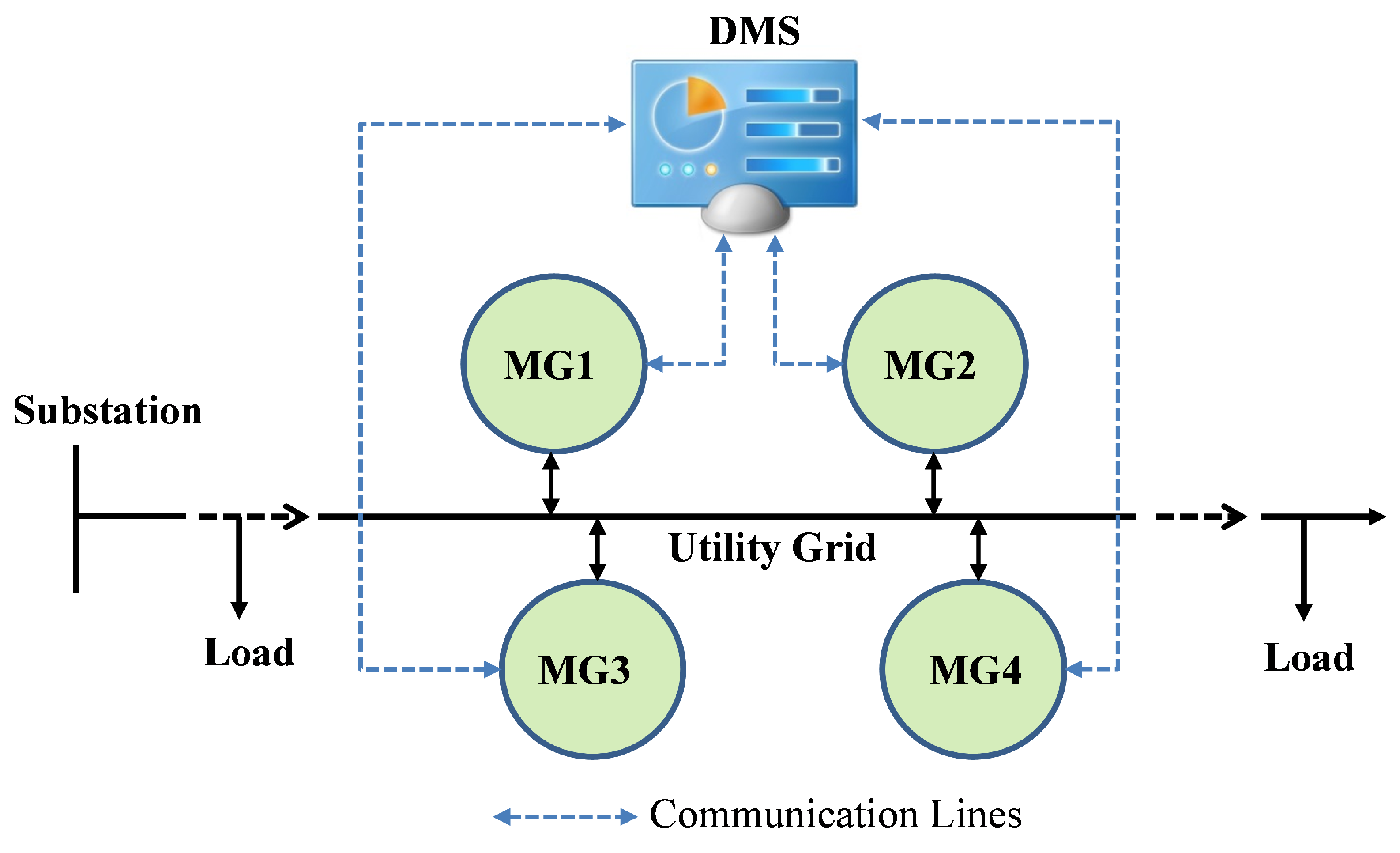
In the past, DGs and ESSs are very rare in distribution grids. Depending on the ownership status, these active components might be directly owned and controlled by the utility or owned by third parties and worked as autonomous entities. Generally, these active components are independent from each other. As the traditional passive distribution network is transforming into a modern active distribution network with the increasing deployment of various types of microgrids, multiple microgrids become interconnected. Under this situation, the mutual influences of them are not neglectable. Nevertheless, these adjacent microgrids could be networked at both communication and control layers and become directly or indirectly interoperable networked microgrids. An example of networked microgrids in the distribution grid is shown in Figure 1. The DMS communicates with each microgrid and coordinates their dispatching. In the proposed distributed energy management, each microgrid makes their own decisions with minimum information exchange. In normal operation, they exchange power with the utility grid for economic benefits and provide various ancillary services, while during utility grid outages, they support each other and provide emergency power to as many loads as possible.

3. Centralized Energy Management

A centralized optimization-based energy management is formulated for networked microgrids coordination in this section as in (1)–(16). The objective is to minimize the total operating cost of the networked microgrids. To be specific, the system total operating costs include the piecewise linear operating cost of DGs in microgrids (line 1), startup costs of DGs in microgrids (line 2), degradation cost of ESSs in microgrids (line 3), load-shedding cost of microgrids (line 4), penalty cost of PV spillage (line 5), penalty cost of wind spillage (line 6), and the energy exchanging cost/benefit at the distribution substation (line 7).

$$\begin{array}{ccc}\hfill min& & \sum _{t=1}^{N_T}\sum _{m=1}^{N_M}\sum _{g=1}^{N_G^m}\left[\sum _{i=1}^{N_I}{\lambda }_{mgt}\left(i\right)p_{mgt}\left(i\right)+{\kappa }_{mg}{u}_{mgt}\right]\hfill \\ & & +\sum _{t=1}^{N_T}\sum _{m=1}^{N_M}\sum _{g=1}^{N_G^m}S{U}_{mgt}\left(u_{mgt},u_{mg,t-1}\right)\hfill \\ & & +\sum _{t=1}^{N_T}\sum _{m=1}^{N_M}\sum _{b=1}^{N_B^m}{C}_{mbt}\left(P_{mbt}^{\mathrm{C}}+P_{mbt}^{\mathrm{D}}\right)\hfill \\ & & {\displaystyle +\sum _{t=1}^{N_T}\sum _{m=1}^{N_M}\sum _{l=1}^{N_L^m}{C}_{mlt}{P}_{mlt}^{LS}}\hfill \\ & & +{\displaystyle \sum _{t=1}^{N_T}\sum _{m=1}^{N_M}\sum _{v=1}^{N_V^m}{C}_{mvt}\left(P_{mvt}^{\mathrm{PV},\max }-P_{mvt}^{\mathrm{PV}}\right)}\hfill \\ & & +{\displaystyle \sum _{t=1}^{N_T}\sum _{m=1}^{N_M}\sum _{w=1}^{N_W^m}{C}_{mwt}\left(P_{mwt}^{\mathrm{W},\max }-P_{mwt}^{\mathrm{W}}\right)}\hfill \\ & & +\sum _{t=1}^{N_T}{\lambda }_t^{\mathrm{SB}}{P}_t^{\mathrm{SB}}\hfill \end{array}$$

(1)

s.t.

$$P_{mgt}=\sum _{i=1}^{N_I}{p}_{mgt}\left(i\right)+u_{mgt}{P}_{mg}^{\min } \forall m,\forall g,\forall t$$

(2)

$$0\le p_{mgt}\left(i\right)\le p_{mg}^{\max }\left(i\right) \forall m,\forall g,\forall t,\forall i$$

(3)

$$u_{mgt}{P}_{mg}^{\min }\le P_{mgt}\le u_{mgt}{P}_{mg}^{\max } \forall m,\forall g,\forall t$$

(4)

$$0\le P_{mbt}^{\mathrm{C}}\le P_{mb}^{\mathrm{C},\max }{u}_{mbt}^{\mathrm{C}} \forall m,\forall b,\forall t$$

(5)

$$0\le P_{mbt}^{\mathrm{D}}\le P_{mb}^{\mathrm{D},\max }{u}_{mbt}^{\mathrm{D}} \forall m,\forall b,\forall t$$

(6)

$$u_{mbt}^{\mathrm{C}}+u_{mbt}^{\mathrm{D}}\le 1 \forall m,\forall b,\forall t$$

(7)

$$SO{C}_{mbt}=SO{C}_{mb,t-1}+P_{mbt}^{\mathrm{C}}{\eta }_{mb}^{\mathrm{C}}▵t-P_{mbt}^{\mathrm{D}}\frac{1}{{\eta }_{mb}^{\mathrm{D}}}▵t \forall m,\forall b,\forall t$$

(8)

$$SO{C}_{mbt}^{\min }\le SO{C}_{mbt}\le SO{C}_{mbt}^{\max } \forall m,\forall b,\forall t$$

(9)

$$0\le P_{mlt}^{LS}\le {\alpha }_{mlt}\%P_{mlt} \forall m,\forall l,\forall t$$

(10)

$$0\le P_{mvt}^{\mathrm{PV}}\le P_{mvt}^{\mathrm{PV},\max } \forall m,\forall v,\forall t$$

(11)

$$0\le P_{mwt}^{\mathrm{W}}\le P_{mwt}^{\mathrm{W},\max } \forall m,\forall w,\forall t$$

(12)

$$\begin{array}{cc}{P}_{mt}^{\mathrm{PCC}}\hfill & +\sum _{g=1}^{N_G^m}{P}_{mgt}+\sum _{b=1}^{N_B^m}\left(P_{mbt}^{\mathrm{D}}-P_{mbt}^{\mathrm{C}}\right)+\sum _{v=1}^{N_V^m}{P}_{mvt}^{\mathrm{PV}}\hfill \\ & +\sum _{w=1}^{N_W^m}{P}_{mwt}^{\mathrm{W}}=\sum _{l=1}^{N_L^m}\left(P_{mlt}-P_{mlt}^{LS}\right) \forall m,\forall t\hfill \end{array}$$

(13)

$$-P_{mt}^{\mathrm{PCC},\max }\le P_{mt}^{\mathrm{PCC}}\le P_{mt}^{\mathrm{PCC},\max } \forall m,\forall t$$

(14)

$$\sum _{m=1}^{N_M}{P}_{mt}^{\mathrm{PCC}}=P_t^{\mathrm{SB}} \forall t$$

(15)

$$-P_t^{\mathrm{SB},\max }\le P_t^{\mathrm{SB}}\le P_t^{\mathrm{SB},\max } \forall t$$

(16)

The objective is subject to constraints of DGs, ESSs, load shedding, microgrid generation–load balance, etc. The cost of dispatchable DGs is estimated through piecewise linearization. The real power of dispatchable DGs is divided into multiple blocks as in (2). The maximum value of each power block is enforced by (3). The real power of DGs is constrained by the minimum and maximum output of DGs as in (4). For ESSs, the charging and discharging power limits of ESSs are enforced by (5) and (6). These two states are mutually exclusive, which is enforced by (7). The state of charge (SOC) of an ESS between any two consecutive time intervals is expressed as (8). The minimum/maximum SOC of ESSs are ensured by (9). The amount of load shedding for each load is limited by a maximum percentage, which is represented in (10). Considering the possible spillage of PV power, the output of PV is limited by its maximum available power during that time period as in (11). Similarly, the output of wind power generation is limited by its maximum available power during that time period as in (12). The power balance of microgrid m is represented as in (13). The power limits of each microgrid at PCC are specified in (14). The overall generation and load balance of networked microgrids is guaranteed by Equation (15). The power injection at the substation is constrained by (16) for peak load reduction or other purposes.

The centralized energy management for the coordination of networked microgrids could be reformulated as a mixed-integer linear programming (MILP) by recasting the startup cost of DGs, i.e., $S{U}_{mgt}$ into mixed-integer linear (MIL) form, then solved by various MILP solvers. Please refer to [37] for details.

4. Distributed Energy Management

As mentioned earlier, the centralized energy management is straightforward to formulate but suffers from computational scalability and privacy issues since the DMS requires access to the information of all components inside the microgrids. This is not allowed in many practical cases because of different ownerships of microgrids. Thus, designing distributed and scalable energy management systems for networked microgrids with customer privacy preserved is imperative.

4.1. ADMM-Based Method

The distributed counterpart of the centralized energy management for networked microgrids is formulated based on the ADMM algorithm [38]. Given that only (15) is complicating constraint involving variables from both the distribution grid level and microgrid level, the ADMM algorithm could be employed to decompose the centralized energy management into subproblems at the DMS level and MCs level. The subproblems are solved by DMS and the corresponding MCs, separately. Their solutions are coordinated through price signals in an iterative way.

$$R_t=P_t^{\mathrm{SB}}-\sum _{m=1}^{N_M}{P}_{mt}^{\mathrm{PCC}} \forall t$$

(17)

First, MCs of microgrids dispatch their internal resources randomly; then, they send their calculated PCC power to DMS. Meanwhile, DMS initializes the price curve and then determines the power injection at the substation. For iteration k, DMS updates the generation–load mismatches (i.e., primal residuals) based on Equation (17) and then sends both primal residuals $R_t^{\left(k\right)}$ and price signals ${\lambda }_t^{\left(k\right)}$ to corresponding MCs. After that, the following two subproblems are solved.

The MCs of each microgrid solve the MCs subproblem as the following:

$$\begin{array}{ccc}\hfill \min & & \sum _{t=1}^{N_T}\sum _{g=1}^{N_G^m}\left[\sum _{i=1}^{N_I}{\lambda }_{mgt}\left(i\right)p_{mgt}\left(i\right)+{\kappa }_{mg}{u}_{mgt}\right]\hfill \\ & & +\sum _{t=1}^{N_T}\sum _{g=1}^{N_G^m}S{U}_{mgt}\left(u_{mgt},u_{mg,t-1}\right)\hfill \\ & & +\sum _{t=1}^{N_T}\sum _{b=1}^{N_B^m}{C}_{mbt}\left(P_{mbt}^{\mathrm{C}}+P_{mbt}^{\mathrm{D}}\right)\hfill \\ & & +\sum _{t=1}^{N_T}\sum _{l=1}^{N_L^m}{C}_{mlt}{P}_{mlt}^{LS}\hfill \\ & & +{\displaystyle \sum _{t=1}^{N_T}\sum _{v=1}^{N_V^m}{C}_{mvt}\left(P_{mvt}^{\mathrm{PV},\max }-P_{mvt}^{\mathrm{PV}}\right)}\hfill \\ & & +{\displaystyle \sum _{t=1}^{N_T}\sum _{w=1}^{N_W^m}{C}_{mvt}\left(P_{mwt}^{\mathrm{W},\max }-P_{mwt}^{\mathrm{W}}\right)}\hfill \\ & & -\sum _{t=1}^{N_T}{\lambda }_t^{\left(k\right)}\left[R_t^{\left(k\right)}+P_{mt}^{\mathrm{PCC},\left(\mathrm{k}\right)}-P_{mt}^{\mathrm{PCC}}\right]\hfill \\ & & +\frac{\rho }{2}{∥{\mathbf{R}}^{\left(k\right)}+{\mathbf{P}}_{\mathbf{m}}^{\mathbf{PCC},\left(\mathbf{k}\right)}-{\mathbf{P}}_{\mathbf{m}}^{\mathbf{PCC}}∥}_2^2\hfill \end{array}$$

(18)

s.t.(2)–(14)

The DMS solves the DMS subproblem as the following:

$$\begin{array}{ccc}\hfill \min & & \sum _{t=1}^{N_T}{\lambda }_t^{\mathrm{SB}}{P}_t^{\mathrm{SB}}\hfill \\ & & -\sum _{t=1}^{N_T}{\lambda }_t^{\left(k\right)}\left[R_t^{\left(k\right)}-P_t^{\mathrm{SB},\left(\mathrm{k}\right)}+P_t^{\mathrm{SB}}\right]\hfill \\ & & +\frac{\rho }{2}{∥{\mathbf{R}}^{\left(k\right)}+{\mathbf{P}}^{\mathbf{SB},\left(\mathbf{k}\right)}-{\mathbf{P}}^{\mathbf{SB}}∥}_2^2\hfill \end{array}$$

(19)

s.t. (16)

After solving all subproblems, MCs send the updated PCC power $P_{mt}^{\mathrm{PCC},\left(\mathrm{k}\right)}$ to DMS; then, DMS updates the primal residual $R_t^{(k+1)}$ and price signal ${\lambda }_t^{(k+1)}$ based on Equation (17) and (20), separately. The k-th iteration is completed. The next iteration begins until convergence.

$$\begin{array}{ccc}\hfill {\lambda }_t^{(k+1)}& =& {\lambda }_t^{\left(k\right)}-\rho R_t^{(k+1)} \forall t\hfill \end{array}$$

(20)

A detailed explanation of the ADMM-based distributed energy management for a networked microgrid is listed in Algorithm 1. Note that both subproblems are formulated as MIQP, which could be solved by commercial MIQP solvers, such as CPLEX or GUROBI.

Algorithm 1 ADMM-based distributed energy management for networked microgrids.

initialization $k\leftarrow 0$. MCs dispatch their internal resources randomly and then send their calculated PCC power to DMS. DMS initializes price curves and then determines the power injection at the substation. repeat DMS updates the primal residual at each bus phase $R_t^{\left(k\right)}$ and sends the two signals $R_t^{\left(k\right)}$ and ${\lambda }_t^{\left(k\right)}$ to corresponding MCs. MCs update the schedules of DGs and ESSs by solving the MCs subproblem. DMS updates the power injection at the substation by solving the DMS subproblem. MCs send the updated PCC power $P_{mt}^{\mathrm{PCC},\left(\mathrm{k}\right)}$ to DMS; then, DMS updates $R_t^{(k+1)}$ and ${\lambda }_t^{(k+1)}$. $k\leftarrow k+1$. until $\left(\left|R_t^{(k+1)}\right|\le R^{\max }\right)$

4.2. MILP-Based Method

As can be seen in (18) and (19), an augmented Lagrange term has been added in the ADMM algorithm to improve the convergence even in the case of non-convex optimization problems. In fact, this added augmented Lagrange term is the square of the Euclidean norm or 2-norm of the primal residual vector in each iteration. By defining a new variable ${\chi }_t=R_t^{\left(k\right)}+P_{mt}^{\mathrm{PCC},\left(\mathrm{k}\right)}-P_{mt}^{\mathrm{PCC}}$, the augmented Lagrange term could be reformulated as a quadratic function of ${\chi }_t$ as shown in (21).

$$\begin{array}{ccc}\hfill {∥\chi ∥}_2^2& & ={∥{\mathbf{R}}^{\left(k\right)}+{\mathbf{P}}_{\mathbf{m}}^{\mathbf{PCC},\left(\mathbf{k}\right)}-{\mathbf{P}}_{\mathbf{m}}^{\mathbf{PCC}}∥}_2^2\hfill \\ & & =\sum _{t=1}^{N_T}{\left(R_t^{\left(k\right)}+P_{mt}^{\mathrm{PCC},\left(\mathrm{k}\right)}-P_{mt}^{\mathrm{PCC}}\right)}^2\hfill \\ & & =\sum _{t=1}^{N_T}{\left({\chi }_t\right)}^2\hfill \end{array}$$

(21)

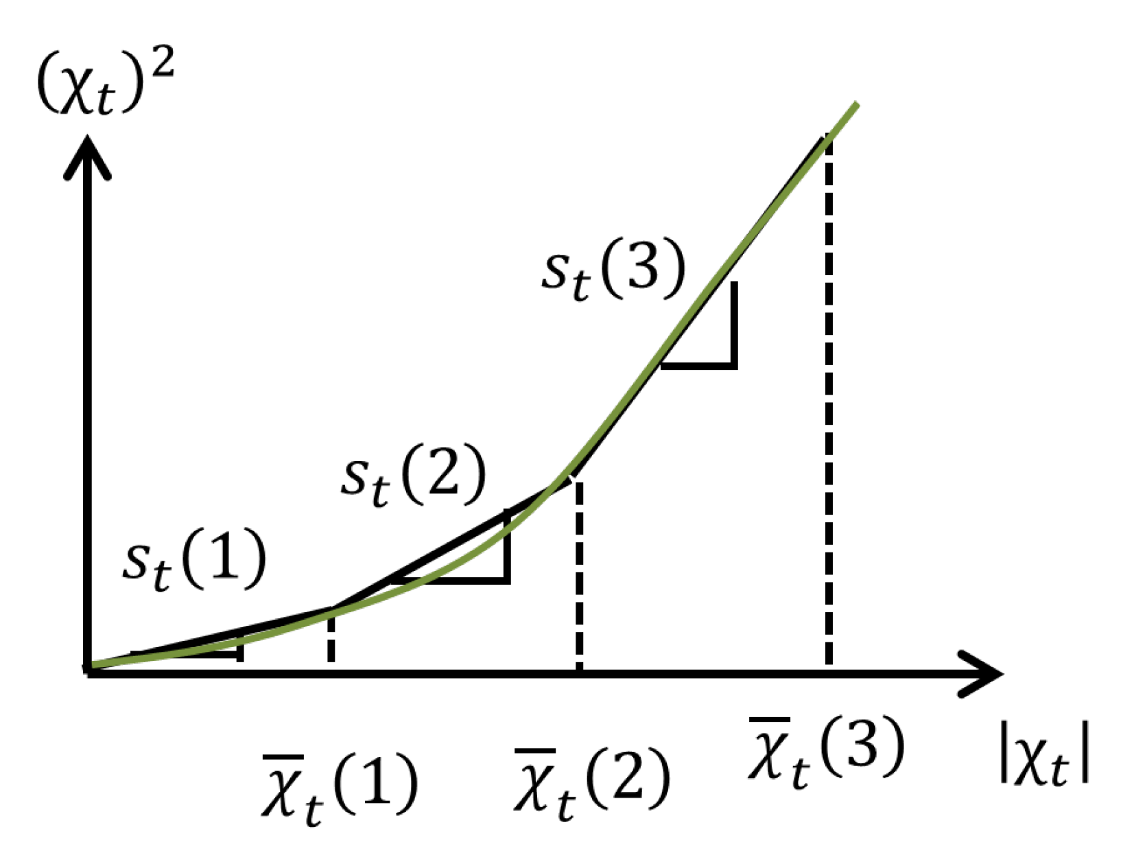
In this paper, a piecewise linearization technique is proposed to approximate the quadratic function of ${\chi }_t$. Since variable ${\chi }_t$ could be positive or negative, we directly linearize its absolute value $\left|{\chi }_t\right|$ as in (22). By dividing $\left|{\chi }_t\right|$ into $N_I$ segments, a linear function is used to approximate the original quadratic function for each segment as shown in Figure 2, where $s_t\left(i\right)$ is the slope of segment i. Thus, the quadratic ${\left({\chi }_t\right)}^2$ could be represented in linear form as in (23). Since the quadratic function is convex, no binary variable is needed here.

Note that the division of linear segments, i.e., determining ${\overline{\chi }}_t\left(1\right),\dots {\overline{\chi }}_t\left(N_I\right)$ and calculation of slope $s_t\left(i\right)$, are performed offline and kept as constants for each iteration. ${\chi }_t\left(i\right)$, i.e., the value of the i-th segment of the piecewise linearization of the quadratic function of ${\chi }_t$, represents new continuous variables, which will be determined at each iteration.

$$\left\{\begin{array}{c}0\le {\chi }_t\left(1\right)\le {\overline{\chi }}_t\left(1\right)\hfill \\ 0\le {\chi }_t\left(2\right)\le {\overline{\chi }}_t\left(2\right)-{\overline{\chi }}_t\left(1\right)\hfill \\ 0\le {\chi }_t\left(3\right)\le {\overline{\chi }}_t\left(3\right)-{\overline{\chi }}_t\left(2\right)\hfill \\ \cdots \hfill \\ 0\le {\chi }_t\left(N_I\right)\le {\overline{\chi }}_t\left(N_I\right)-{\overline{\chi }}_t\left(N_I-1\right)\hfill \\ \sum _{i=1}^{N_I}{\chi }_t\left(i\right)\ge {\chi }_t,\sum _{i=1}^{N_I}{\chi }_t\left(i\right)\ge -{\chi }_t\hfill \\ \left|{\chi }_t\right|=\sum _{i=1}^{N_I}{\chi }_t\left(i\right)\hfill \end{array}\right.$$

(22)

$${\left({\chi }_t\right)}^2=\sum _{i=1}^{N_I}{\chi }_t\left(i\right)s_t\left(i\right) \forall t$$

(23)

With the proposed piecewise linearization technique, the original MIQP-based MCs subproblem as in (18) could be transformed into MILP as in (24).

$$\begin{array}{ccc}\hfill \min & & \sum _{t=1}^{N_T}\sum _{g=1}^{N_G^m}\left[\sum _{i=1}^{N_I}{\lambda }_{mgt}\left(i\right)p_{mgt}\left(i\right)+{\kappa }_{mg}{u}_{mgt}\right]\hfill \\ & & +\sum _{t=1}^{N_T}\sum _{g=1}^{N_G^m}S{U}_{mgt}\left(u_{mgt},u_{mg,t-1}\right)\hfill \\ & & +\sum _{t=1}^{N_T}\sum _{b=1}^{N_B^m}{C}_{mbt}\left(P_{mbt}^{\mathrm{C}}+P_{mbt}^{\mathrm{D}}\right)\hfill \\ & & +\sum _{t=1}^{N_T}\sum _{l=1}^{N_L^m}{C}_{mlt}{P}_{mlt}^{LS}\hfill \\ & & +{\displaystyle \sum _{t=1}^{N_T}\sum _{v=1}^{N_V^m}{C}_{mvt}\left(P_{mvt}^{\mathrm{PV},\max }-P_{mvt}^{\mathrm{PV}}\right)}\hfill \\ & & +{\displaystyle \sum _{t=1}^{N_T}\sum _{w=1}^{N_W^m}{C}_{mvt}\left(P_{mwt}^{\mathrm{W},\max }-P_{mwt}^{\mathrm{W}}\right)}\hfill \\ & & -\sum _{t=1}^{N_T}{\lambda }_t^{\left(k\right)}\left[R_t^{\left(k\right)}+P_{mt}^{\mathrm{PCC},\left(\mathrm{k}\right)}-P_{mt}^{\mathrm{PCC}}\right]\hfill \\ & & +\frac{\rho }{2}\sum _{t=1}^{N_T}\sum _{i=1}^{N_I}{\chi }_t\left(i\right)s_t\left(i\right)\hfill \end{array}$$

(24)

s.t. (2)–(14), and (21)–(23)

Similarly, the original MIQP-based DMS subproblem as in (19) could be transformed into MILP as in (25).

$$\begin{array}{ccc}\hfill \min & & \sum _{t=1}^{N_T}{\lambda }_t^{\mathrm{SB}}{P}_t^{\mathrm{SB}}\hfill \\ & & -\sum _{t=1}^{N_T}{\lambda }_t^{\left(k\right)}\left[R_t^{\left(k\right)}-P_t^{\mathrm{SB},\left(\mathrm{k}\right)}+P_t^{\mathrm{SB}}\right]\hfill \\ & & +\frac{\rho }{2}\sum _{t=1}^{N_T}\sum _{i=1}^{N_I}{\chi }_t\left(i\right)s_t\left(i\right)\hfill \end{array}$$

(25)

s.t. (16), and (21)–(23)

It should be noted that the solution procedure of the proposed MILP-based distributed energy management for the coordination of networked microgrids is the same as in Algorithm 1, except the subproblems are all MILP as in (24) and (25), which could be solved more efficiently by either commercial or open-source MILP solvers.

Both commercial (e.g., CPLEX and GUROBI) and open-source (e.g., CBC) MILP solvers utilize the branch and cut algorithm to solve MILP problems [39]. It is a very successful algorithm for solving a variety of integer programming problems, and it also can provide a guarantee of optimality. The branch and cut algorithm is the exact algorithm consisting of a combination of a cutting plane method and a branch and bound algorithm.

It should also be noted that ADMM cannot guarantee the global optimum for non-convex optimization problems. Nevertheless, ADMM can usually converge with modest accuracy within a few tens of iterations [38]. The proposed MILP-based distribution energy management equivalently linearizes the augmented Lagrange term in ADMM; thus, it has the same convergence property as ADMM. Therefore, the proposed MILP-based distribution energy management should converge with modest accuracy within a few tens of iterations.

5. Case Studies

5.1. Test System

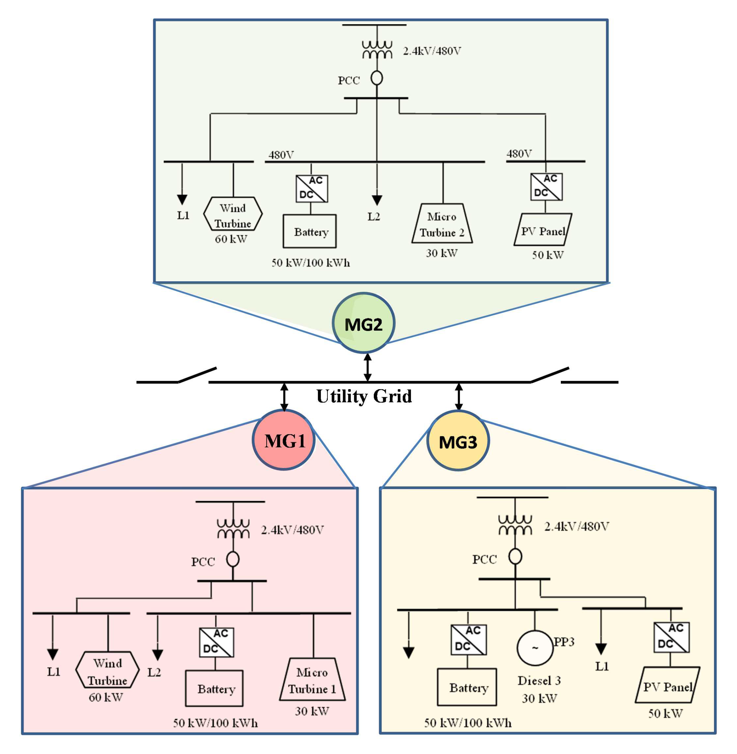
The proposed distributed energy management for the coordination of networked microgrids is demonstrated on a modified Oak Ridge National Laboratory (ORNL) Distributed Energy Control and Communication (DECC) networked microgrids test system, as shown in Figure 3 [17]. This system consists of three microgrids. Both dispatchable DGs and renewable generation as well as batteries are installed in the network microgrids test system. Both wind and PV inverters are controlled using the maximum power point tracker (MPPT) with curtailment available upon requested by the MCs. More details on the control and power of the ORNL DECC networked microgrids could be found in [40].

The parameters of dispatchable DGs are listed in

Table 2. Parameters of dispatchable DGs.

DG Type	${\mathbf{P}}^{\mathbf{min}}$ (kW)	${\mathbf{P}}^{\mathbf{max}}$ (kW)	Start-Up Cost ($)	Cost at ${\mathbf{P}}^{\mathbf{min}}$ ($/h)	${\mathit{\lambda }}_{\mathit{m}\mathit{g}\mathit{t}}\left(1\right)$ ($/kWh)	${\mathit{\lambda }}_{\mathit{m}\mathit{g}\mathit{t}}\left(2\right)$ ($/kWh)	${\mathit{\lambda }}_{\mathit{m}\mathit{g}\mathit{t}}\left(3\right)$ ($/kWh)
Microturbine 1	10	30	1	3.39	0.2172	0.2644	0.3016
Microturbine 2	10	30	1	2.31	0.1324	0.1552	0.1880
Diesel 3	10	30	1.5	2.68	0.1284	0.1412	0.1541

. The costs function of DGs between the minimum power output and maximum power output are equally divided into three blocks. The linear marginal cost of each block is shown in Table 2.

The parameters of batteries are listed in

Table 3. Parameters of batteries.

Battery Type	Power Capacity (kW)	Energy Capacity (kWh)	${\mathbf{SOC}}^{\mathbf{max}}$ (%)	${\mathbf{SOC}}^{\mathbf{min}}$ (%)
Lithium ion	10	20	95	25
Degradation Cost ($/kWh)	Charging Efficiency (%)	Discharging Efficiency (%)	Initial SOC (%)	End SOC (%)
0.02	0.95	0.95	50	50

. Without loss of generality, these three batteries are assumed to be identical.

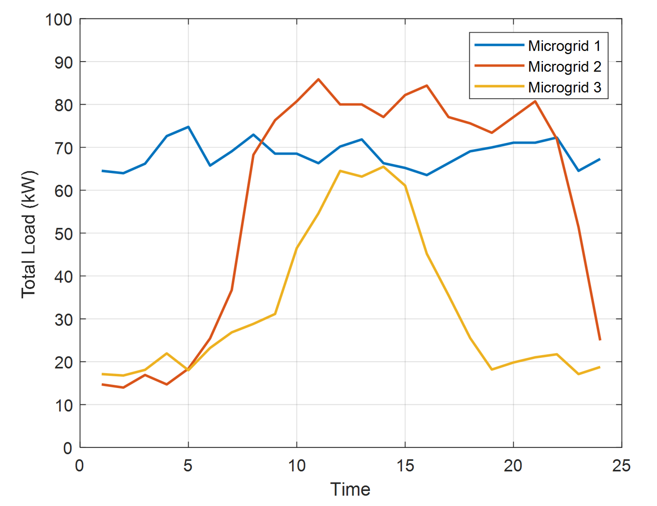
The forecasted wind and PV power of the three microgrids are directly taken from [17]. The total load of each microgrid is forecasted as in Figure 4. For each microgrid, the total load is equally divided into two loads. The maximum percentage of load shedding is assumed to be 80%. The cost of load shedding is assumed to be 1 $/kWh.

The hourly utility rates, i.e., prices of energy supplied by the utility at the distribution substation, are shown in

Table 4. Utility rates.

Hour	${\mathit{\lambda }}^{\mathbf{SB}}$ (ct/kWh)	Hour	${\mathit{\lambda }}^{\mathbf{SB}}$ (ct/kWh)	Hour	${\mathit{\lambda }}^{\mathbf{SB}}$ (ct/kWh)
1	8.65	9	12.0	17	16.42
2	8.11	10	9.19	18	9.83
3	8.25	11	12.3	19	8.63
4	8.10	12	20.7	20	8.87
5	8.14	13	26.82	21	8.35
6	8.13	14	27.35	22	16.44
7	8.34	15	13.81	23	16.19
8	9.35	16	17.31	24	8.87

[41]. The utility rates are normally provided by the utility operator and used as input to the proposed distributed energy management system. For each microgrid, the maximum power at PCC is assumed to be 200 kW.

The time span of case studies is set as one day, i.e., 24 h, with hourly resolution. The initial price is set as 0.1 $/kWh for the whole scheduling horizon. The penalty factor $\rho$ is assumed to be 0.1. The optimization model is programmed in MATLAB and solved by the mixed-integer quadratic programming (MIQP) solver CPLEX 12.6 and open-source MILP solver CBC, separately.

5.2. Comparing Costs and Solution Time of Different Cases

The total costs of networked microgrids calculated by centralized energy management, ADMM-based distributed energy and the proposed MILP-based distributed energy management in both grid-connected and islanded modes are listed in

Table 5. Comparison of costs and solution time of different methods.

Cases		Total Operating Costs ($)	Solution Time (Seconds)
Grid-connected	Centralized	190.37	2.81
	ADMM-based Distributed	190.78	57.36
	MILP-based Distributed	190.65	54.92
Islanded	Centralized	377.41	2.43
	ADMM-based Distributed	378.25	48.77
	MILP-based Distributed	378.07	40.85

. Comparing with the results of centralized energy management, the total operating costs calculated by both ADMM-based and MILP-based distributed energy management are slightly increased (less than 0.5%) in both grid-connected and islanded modes. In other words, both ADMM-based and proposed MILP-based distributed energy management could reach the same level of optimality as centralized energy management. These tiny differences of objective function values between centralized and distributed methods are due to the fact that the distributed optimization cannot guarantee a global optimum for non-convex optimization problems.

The solution times of centralized energy management, ADMM-based distributed energy and the proposed MILP-based distributed energy management in both grid-connected and islanded modes are compared in Table 5. It can be obviously seen that the solution time of centralized optimization is the least due to the relatively small size of the problem. Comparing the solution time between ADMM-based and MILP-based distributed energy management, the MILP-based distributed energy management is a little better than ADMM-based distributed energy management. This is largely due to the fact that MILP models could be more efficiently solved than MIQP models. More importantly, the proposed MILP-based method could be efficiently solved by a free and open-source MILP solver, which could facilitate the deployment of networked microgrids.

5.3. Convergence of Distributed Energy Management

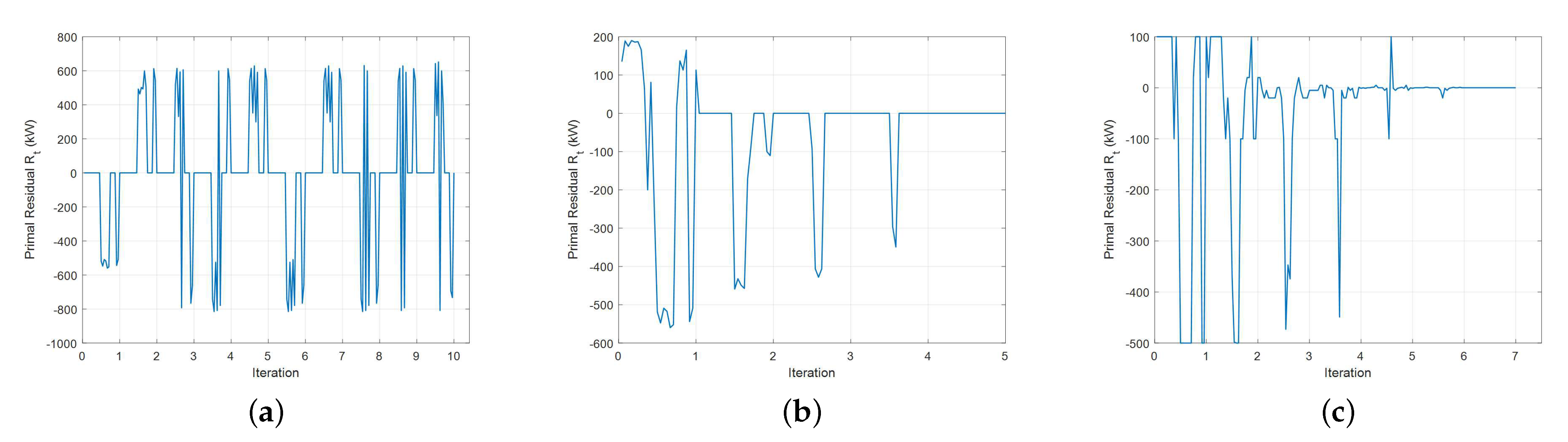
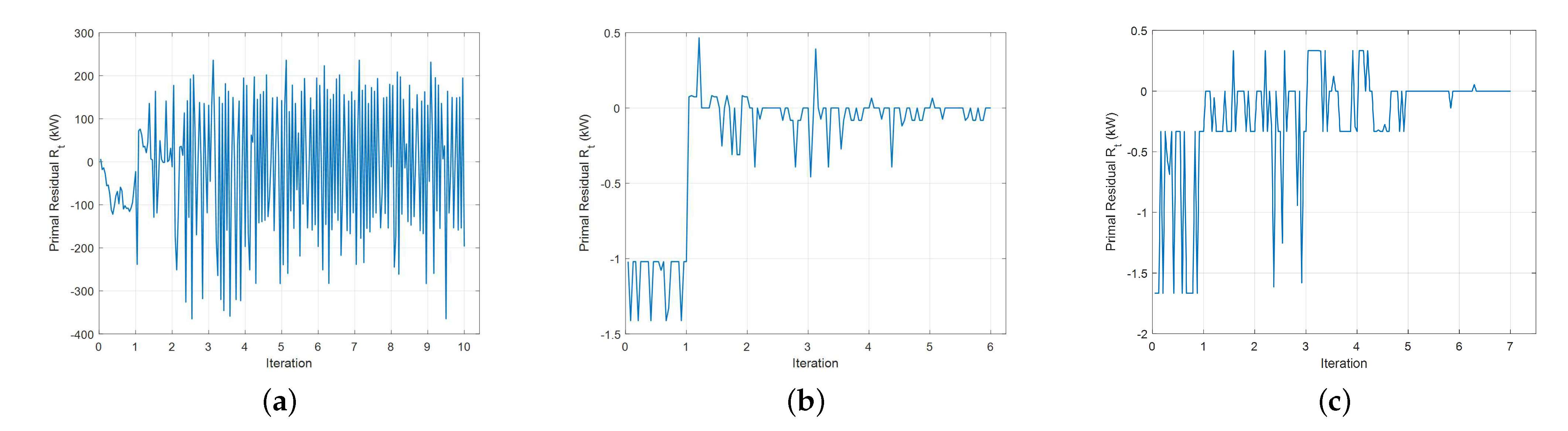
A reasonable stopping criterion for the distributed energy management is that the generation–load mismatch $R_t$ should be small enough [38], i.e., the generation and consumption are well balanced for any time interval. The unbalanced power $R_t$ could be calculated according to Equation (17). The stopping criteria used in this work is $\left|R_t\right|\le 0.1$ kW. To investigate the effects of different types of Lagrange terms on the convergence of the distributed energy management, three types of Lagrange terms of $R_t$, i.e., square of one-norm, square of two-norm (ADMM), and linearized square of two-norm (proposed MILP-based method), are tested for both grid-connected and islanded mode.

The converging process of distributed methods with different types of Lagrange terms in grid-connected and islanded mode are compared in Figure 5 and Figure 6, separately. As can be seen, the square of one-norm type of Lagrange term cannot yield convergence, while both the square of two-norm and linearized square of two-norm types of Lagrange term yield convergence in less than 10 iterations. Note that the ADMM can be very slow to converge to high accuracy. However, it is often the case that ADMM converges to modest accuracy within a few tens of iterations [38]. In addition, the proposed MILP-based distributed energy management with linearized square of two-norm type of Lagrange term has the same convergence property as ADMM with square of two-norm type of Lagrange term.

As can be seen in Figure 5 and Figure 6, the calculated generation–load mismatch $R_t$ for each iteration is alternating between positive and negative values. If $R_t$ is positive, the power supply at the distribution substation is greater than the total power consumption of all microgrids through PCC based on (17). Then, according to (20), the price will be reduced, leading to more power consumption and less power supply in the next generation. While $R_t$ is negative, i.e., the power supply at the distribution substation is less than the total power consumption of all microgrids through PCC based on (17). According to (20), the price will be increased, leading to less power consumption and more power supply in the next generation. If the algorithm is convergent, the magnitude of generation–load mismatch $R_t$ will be reduced every iteration and eventually converges to a very small value; i.e., the generation and load are balanced.

5.4. Solutions of MILP-Based Distributed Energy Management

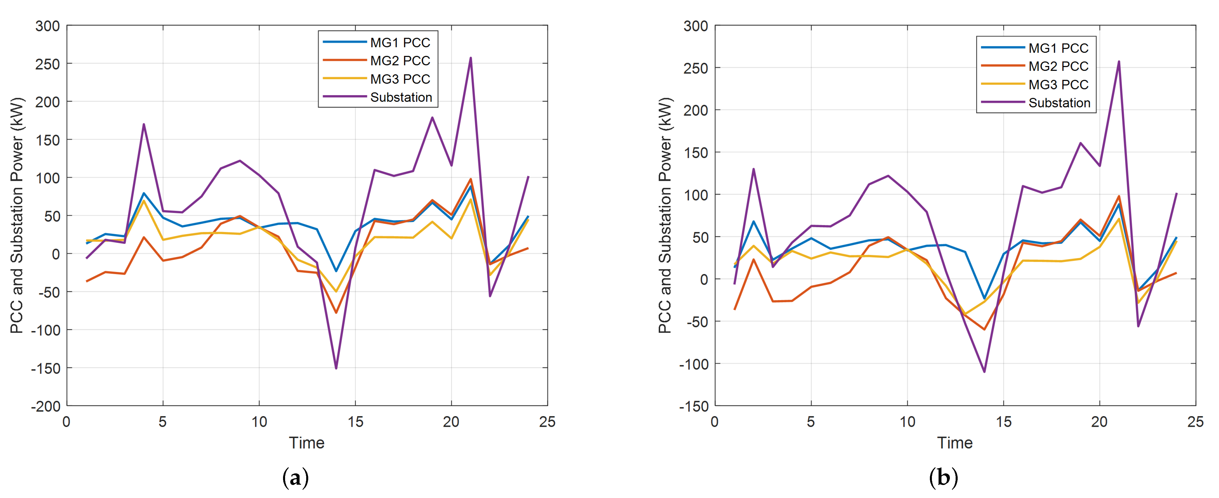
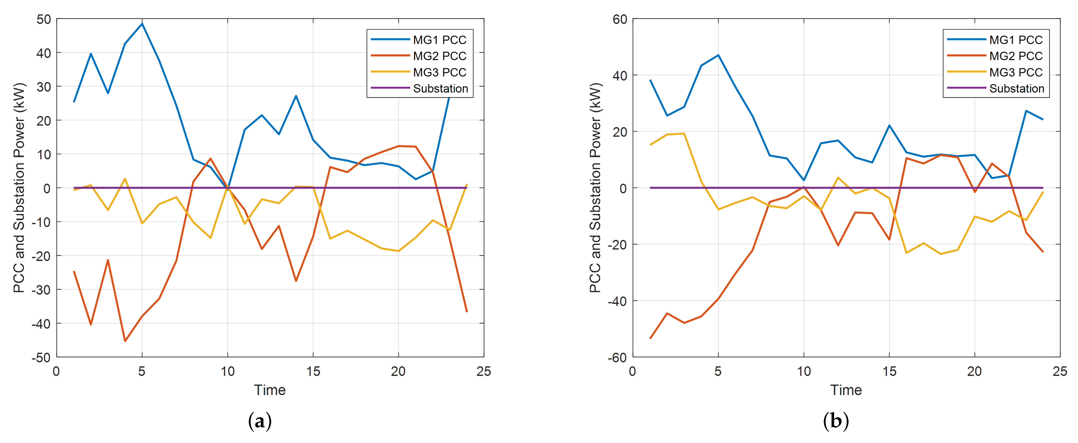
To further validate the accuracy of the proposed MILP-based distributed energy management for the coordination of networked microgrids, the PCC power of each microgrid and power injection at the substation in both grid-connected and islanded modes are compared between the proposed MILP-based distributed energy management and the centralized energy management in Figure 7 and Figure 8, separately.

Generally, the results of the proposed MILP-based distributed energy management are the same as those of the centralized energy management except for some tiny differences. In grid-connected mode, as can be seen in Figure 7, the networked microgrids export power to the utility grid during the early afternoon when the PV power is high, while they import power from the utility grid during the evening and night when the PV power is zero. In islanded mode, as can be seen in Figure 8, the power injection at the substation bus is forced to be zero. Thus, the PCC power of all networked microgrids are complementary; i.e., the summation of them always equals zero.

Although the results of proposed MILP-based distributed energy management generally follow the same trend as the results of centralized energy management, there are some differences. For example, the total power injection at the substation by microgrids in grid-connected mode is around 150 kW by the centralized energy management, as shown in Figure 7a. However, the same injected power calculated by the proposed MILP-based distributed energy management is around 110 kW, as shown in Figure 7b. This issue also exists in the results of islanded mode. This is due to the fact that the proposed MILP-based distributed energy management has the same convergence property as ADMM, which cannot guarantee converging to the global optimal for non-convex problems.

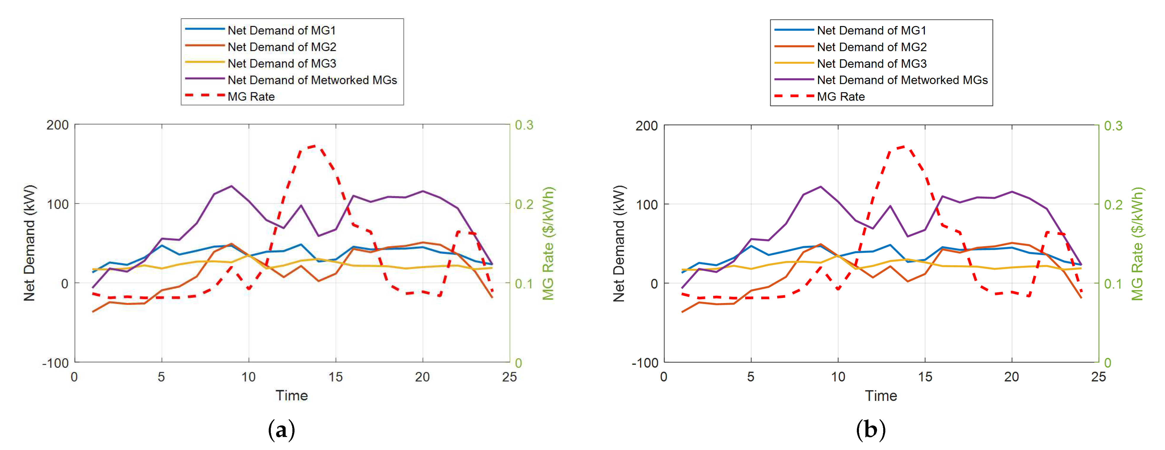
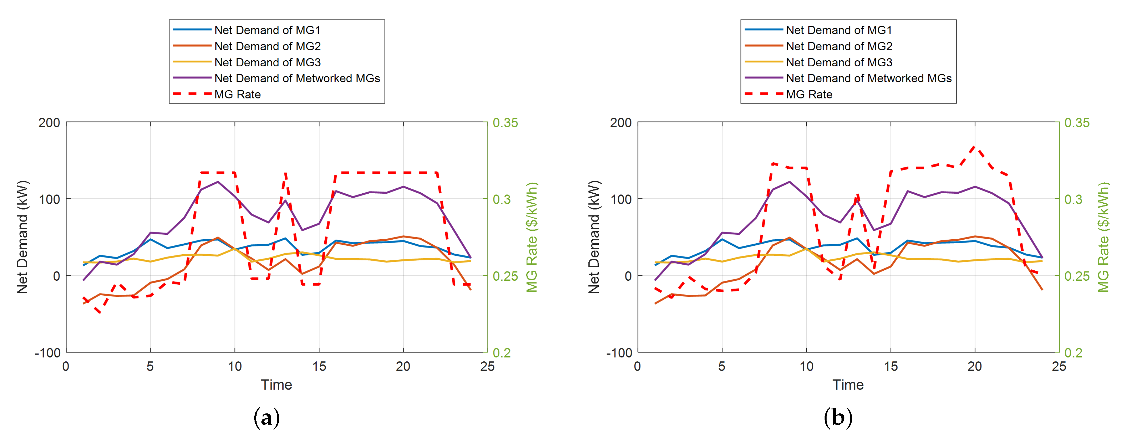
The converged price signal in both grid-connected and islanded modes is compared between the proposed MILP-based distributed energy management and the ADMM-based distributed energy management in Figure 9 and Figure 10, separately. Generally, the results of the proposed MILP-based distributed energy management are the same as those of the ADMM-based distributed energy management except for some small differences. The net demand of each microgrid, i.e., total load minus renewable generation, and net demand of network microgrids, i.e., the summation of net demand of all microgrids, have also been calculated and shown in Figure 9 and Figure 10.

In grid-connected mode, the converged price signal and net demand of microgrids are shown in Figure 9. As can be seen, the converged price signal has very little to do with the total net demand of networked microgrids, but it mainly follows the utility rates at the distribution substation. This is due to the fact that the utility rate at the distribution substation bus is generally much lower than the marginal generation cost of DGs except for peak price hours (Hour 12–14 and hour 22–23) as shown in Table 2 and Table 4. Meanwhile, during peak price hours, the DGs with lower marginal cost than the utility rate are committed at rated power. The distribution substation bus will cover the rest of the demands like a slack bus. Thus, the converged price signal is generally the same as the utility rates at the distribution substation.

In islanded mode, the converged price signal generally follows the profile of net demand of the networked microgrids, as shown in Figure 10. Since the power injection at the substation bus is forced to be zero in islanded mode, the net demand of networked microgrids is purely supplied by the dispatchable DGs in the system. As a result, the profiles of the converged price and total net demand match very well, as presented in Figure 10. With greater total net demand, the DGs with higher marginal cost needs to be committed. Thus, the converged price is higher. The peak price corresponds to the peak net demand.

6. Conclusions

An MILP-based distributed energy management for the coordination of networked microgrids is proposed in this paper. Given the price signals and the generation–load mismatch, the microgrid controllers (MCs) and distribution management system (DMS) update their schedules, separately. Then, the price signals and generation–load mismatch are updated and distributed for another iteration until convergence. The proposed distributed energy management coordinates various microgrids and the utility grid with generation–load balance guaranteed and microgrid customers’ privacy preserved. In particular, a piecewise linearization technique is employed to approximate the augmented Lagrange term in the ADMM and transform the MIQP subproblems into MILP, which could be solved more efficiently and by open-source solvers. The soundness, accuracy and efficiency of the proposed model are proved with the results of various case studies.

Future work includes integrating the operational objectives and constraints of the distribution grid into the proposed model, e.g., volt/var optimization (VVO), loss reduction, power flow constraints, power factor constraints, voltage constraints, phase balance constraints, even stability constraints in islanded mode, etc. In addition, to keep the distributed energy management in MILP format, techniques to linearize these objectives and constraints will be investigated.

References

- Khan, M.Z.; Mu, C.; Habib, S.; Alhosaini, W.; Ahmed, E.M. An Enhanced Distributed Voltage Regulation Scheme for Radial Feeder in Islanded Microgrid. Energies 2021, 14, 6092. [Google Scholar] [CrossRef]
- Park, B.; Zhang, Y.; Olama, M.; Kuruganti, T. Model-free control for frequency response support inmicrogrids utilizing wind turbines. Electr. Power Syst. Res. 2021, 194, 107080. [Google Scholar] [CrossRef]
- Liu, R.; Wang, S.; Liu, G.; Wen, S.; Zhang, J.; Ma, Y. An Improved Virtual Inertia Control Strategy for Low Voltage AC Microgrids with Hybrid Energy Storage Systems. Energies 2022, 15, 442. [Google Scholar] [CrossRef]
- Nematollahi, A.F.; Shahinzadeh, H.; Nafisi, H.; Vahidi, B.; Amirat, Y.; Benbouzid, M. Sizing and Sitting of DERs in Active Distribution Networks Incorporating Load Prevailing Uncertainties Using Probabilistic Approaches. Appl. Sci. 2021, 11, 4156. [Google Scholar] [CrossRef]
- Cagnano, A.; De Tuglie, E.; Mancarella, P. Microgrids: Overview and guidelines for practical implementations and operation. Appl. Energy 2020, 258, 114039. [Google Scholar] [CrossRef]
- Bagherzadeh, L.; Shahinzadeh, H.; Shayeghi, H.; Gharehpetian, G.B. A short-term energy management of microgrids considering renewable energy resources, micro-compressed air energy storage and DRPs. Int. J. Renew. Energy Res. 2019, 9, 1712–1723. [Google Scholar]
- Liu, G.; Jiang, T.; Ollis, T.B.; Li, X.; Li, F.; Tomsovic, K. Resilient distribution system leveraging distributed generation and microgrids: A review. IET Energy Syst. Integr. 2020, 2, 289–304. [Google Scholar] [CrossRef]
- Hirsch, A.; Parag, Y.; Guerrero, J. Microgrids: A review of technologies, key drivers, and outstanding issues. Renew. Sustain. Energy Rev. 2018, 90, 402–411. [Google Scholar] [CrossRef]
- Chen, B.; Wang, J.; Lu, X.; Chen, C.; Zhao, S. Networked Microgrids for Grid Resilience, Robustness, and Efficiency: A Review. IEEE Trans. Smart Grid 2021, 12, 18–32. [Google Scholar] [CrossRef]
- Zou, H.; Mao, S.; Wang, Y.; Zhang, F.; Chen, X.; Cheng, L. A Survey of Energy Management in Interconnected Multi-Microgrids. IEEE Access 2019, 7, 72158–72169. [Google Scholar] [CrossRef]
- Islam, M.; Yang, F.; Amin, M. Control and optimisation of networked microgrids: A review. IET Renew Power Gener. 2021, 15, 1133–1148. [Google Scholar] [CrossRef]
- Xie, H.; Wang, W.; Wang, W.; Tian, L. Optimal Dispatching Strategy of Active Distribution Network for Promoting Local Consumption of Renewable Energy. Front. Energy Res. 2022, 10, 826141. [Google Scholar] [CrossRef]
- Wang, Z.; Chen, B.; Wang, J.; Begovic, M.; Chen, C. Coordinated Energy Management of Networked Microgrids in Distribution Systems. IEEE Trans. Smart Grid 2015, 6, 45–53. [Google Scholar] [CrossRef]
- Hussain, A.; Bui, V.H.; Kim, H.M. A Resilient and Privacy- Preserving Energy Management Strategy for Networked Microgrids. IEEE Trans. Smart Grid 2018, 9, 2127–2139. [Google Scholar] [CrossRef]
- Huang, Y.; Ju, Y.; Ma, K.; Short, M.; Chen, T.; Zhang, R.; Lin, Y. Three-phase optimal power flow for networked microgrids based on semidefinite programming convex relaxation. Appl. Energy 2021, 305, 117771. [Google Scholar] [CrossRef]
- Haghifam, S.; Najafi-Ghalelou, A.; Zare, K.; Shafiekhah, M.; Arefi, A. Stochastic bi-level coordination of active distribution network and renewable-based microgrid considering eco-friendly Compressed Air Energy Storage system and Intelligent Parking Lot. J. Clean. Prod. 2021, 278, 122808. [Google Scholar] [CrossRef]
- Liu, G.; Ollis, T.B.; Ferrari, M.F.; Sundararajan, A.; Tomsovic, K. Robust Scheduling of Networked Microgrids for Economics and Resilience Improvement. Energies 2022, 15, 2249. [Google Scholar] [CrossRef]
- Choobineh, M.; Mohagheghi, S. Robust Optimal Energy Pricing and Dispatch for a Multi-Microgrid Industrial Park Operating Based on Just-In-Time Strategy. IEEE Trans. Ind. Appl. 2019, 55, 3321–3330. [Google Scholar] [CrossRef]
- Long, Y.; Li, Y.; Wang, Y. Low-carbon economic dispatch considering integrated demand response and multistep carbon trading for multi-energy microgrid. Sci. Rep. 2022, 12, 6218. [Google Scholar] [CrossRef]
- Warner, J.D.; Masaud, T.M. Decentralized Peer-to-Peer Energy Trading Model for Networked Microgrids. In Proceedings of the 2021 IEEE Conference on Technologies for Sustainability (SusTech), Virtual, 22–24 April 2021; pp. 1–6. [Google Scholar]
- Anoh, K.; Maharjan, S.; Ikpehai, A.; Zhang, Y.; Adebisi, B. Energy peer-to-peer trading in virtual microgrids in smart grids: A game-theoretic approach. IEEE Trans. Smart Grid 2020, 11, 1264–1275. [Google Scholar] [CrossRef]
- Rahbar, K.; Chai, C.; Zhang, R. Energy cooperation optimization in microgrids with renewable energy integration. IEEE Trans. Smart Grid 2018, 9, 1482–1493. [Google Scholar] [CrossRef]
- Malekpour, A.R.; Pahwa, A. Stochastic networked microgrid energy management with correlated wind generators. IEEE Trans. Power Syst. 2017, 32, 3671–3693. [Google Scholar] [CrossRef]
- La Bella, A.; Falsone, A.; Ioli, D.; Prandini, M.; Scattolini, R. A mixed-integer distributed approach to prosumers aggregation for providing balancing services. Int. J. Electr. Power Energy Syst. 2021, 133, 107228. [Google Scholar] [CrossRef]
- Liu, G.; Ollis, B.; Xiao, B.; Zhang, X.; Tomsovic, K. Distributed Energy management for Community Microgrids Considering Phase balancing and peak Shaving. IET Gener. Transm. Distrib. 2019, 13, 1612–1620. [Google Scholar] [CrossRef]
- Feng, C.; Wen, F.; Zhang, L.; Xu, C.; Salam, M.A.; You, S. Decentralized Energy Management of Networked Microgrid Based on Alternating-Direction Multiplier Method. Energies 2018, 11, 2555. [Google Scholar] [CrossRef]
- Zhou, X.; Ai, Q. An integrated two-level distributed dispatch for interconnected microgrids considering unit commitment and transmission loss. J. Renew. Sust. Energ. 2019, 11, 025504. [Google Scholar] [CrossRef]
- Liu, T.; Tan, X.; Sun, B.; Wu, Y.; Tsang, D. Energy management of cooperative microgrids: A distributed optimization approach. Int. J. Electr. Power Energy Syst. 2018, 96, 335–346. [Google Scholar] [CrossRef]
- Liu, G.; Jiang, T.; Ollis, T.B.; Zhang, X.; Tomsovic, K. Distributed energy management for community microgrids considering network operational constraints and building thermal dynamics. Appl. Energy 2019, 239, 83–95. [Google Scholar] [CrossRef]
- La Bella, A.; Farina, M.; Sandroni, C.; Scattolini, R. Design of aggregators for the day-ahead management of microgrids providing active andreactive power services. IEEE Trans. Control Syst Technol. 2020, 28, 2616–2624. [Google Scholar] [CrossRef]
- Velasquez, M.A.; Torres-Perez, O.; Quijano, N.; Cadena, A. Hierarchical dispatch of multiple microgrids using nodal price: An approach from consensus and replicator dynamics. J. Mod. Power Syst. Clean Energy 2019, 7, 1573–1584. [Google Scholar] [CrossRef]
- The ILOG CPLEX Website. 2022. Available online: http://www-01.ibm.com/software/commerce/optimization/cplex-optimizer/index.html (accessed on 18 September 2022).
- Gurobi Optimizer. 2022. Available online: https://www.gurobi.com/products/gurobi-optimizer/ (accessed on 18 September 2022).
- CBC User Guide. 2022. Available online: https://www.coin-or.org/Cbc/cbcuserguide.html (accessed on 18 September 2022).
- Hanifi, S.; Liu, X.; Lin, Z.; Lotfian, S. A Critical Review of Wind Power Forecasting Methods—Past, Present and Future. Energies 2020, 13, 3764. [Google Scholar] [CrossRef]
- Sundararajan, A.; Ollis, B. Regression and Generalized Additive Model to Enhance the Performance of Photovoltaic Power Ensemble Predictors. IEEE Access 2021, 9, 111899–111914. [Google Scholar] [CrossRef]
- Liu, G.; Ollis, T.B.; Xiao, B.; Zhang, X.; Tomsovic, K. Community Microgrid Scheduling Considering Network Operational Constraints and Building Thermal Dynamics. Energies 2017, 13, 1554. [Google Scholar] [CrossRef]
- Boyd, S.; Parikh, N.; Chu, E.; Peleato, B.; Eckstein, E. Distributed Optimization and Statistical Learning via the Alternating Direction Method of Multipliers. Found. Trends Mach. Learn. 2011, 3, 1–122. [Google Scholar] [CrossRef]
- Mitchell, J.E. Branch-and-Cut Algorithms for Combinatorial Optimization Problems; Oxford University Press: Oxford, UK, 2002; pp. 1–19. [Google Scholar]
- Xiao, B.; Starke, M.; Liu, G.; Ollis, B.; Irminger, P.; Dimitrovski, A.; Prabakar, K.; Dowling, K.; Xu, Y. Development of hardware-in-the-loop microgrid testbed. In Proceedings of the IEEE Energy Conversion Congress & Exposition (ECCE 2015), Montreal, QC, Canada, 20–24 September 2015; pp. 1196–1202. [Google Scholar]
- Liu, G.; Xu, Y.; Tomsovic, K. Bidding Strategy for Microgrid in Day-Ahead Market Based on Hybrid Stochastic/Robust Optimization. IEEE Trans. Smart Grid 2016, 7, 227–237. [Google Scholar] [CrossRef]
Figure 1.
Example of networked microgrids.
Figure 2.
Piecewise linearization of a quadratic function.
Figure 3.
Modified ORNL DECC networked microgrids test system.
Figure 4.
Load of each microgrid.
Figure 5.
The generation–load mismatch of different methods in grid-connected mode. (a) Square of 1-norm. (b) Square of 2-norm. (c) Linearized square of 2-norm.
Figure 6.
The generation–load mismatch of different methods in islanded mode. (a) Square of 1-norm. (b) Square of 2-norm. (c) Linearized square of 2-norm.
Figure 7.
Calculated PCC power by different methods in grid-connected mode. (a) Centralized optimization. (b) MILP-based distributed optimization.
Figure 8.
Calculated PCC power by different methods in islanded mode. (a) Centralized optimization. (b) MILP-based distributed optimization.
Figure 9.
Converged price signal and net demand of networked microgrids by different distributed methods in grid-connected mode. (a) ADMM-based distributed optimization. (b) MILP-based distributed optimization.
Figure 10.
Converged price signal and net demand of networked microgrids by different distributed methods in islanded mode. (a) ADMM-based distributed optimization. (b) MILP-based distributed.