Heat Transfer and Fluid Circulation of Thermoelectric Fluid through the Fractional Approach Based on Local Kernel

Abstract

A thermoelectric effect occurs when a material’s intrinsic property directly converts temperature differences applied across its body into electric voltage. This manuscript presents the prediction for maximum and optimal heat transfer efficiency of a thermoelectric fluid via the non-classical approach of the differential operator. The fractionalized mathematical model is also established to analyze the efficiency and characteristics of thermoelectric fluid through a temperature distribution and velocity field. The comprehensive analytical approach of integral transforms and Cardano’s method are applied to provide analytical solutions that include the dynamic investigation of the temperature distribution and velocity field. A dynamic investigation of the temperature distribution and velocity field of the thermoelectric fluid is explored on the basis of magnetization and anti-magnetization, which describe the behavior for sine and cosine sinusoidal waves. The rheological parameter, i.e., magnetization, suggests that by employing varying magnetic fields, the magnetized intensity generates 34.66% of the magnetic hysteresis during the thermoelectric effect.

1. Introduction

It is a well-established fact that thermal analysis of various materials has become the central point for various thermal industries and technologies due to enhancing power density. The performance of various power devices in many industries depends upon the interplay among thermal, optical and electronic sensation. Various thermal industries and technologies desire thermoelectric devices for obtaining electrical and thermal stability, due to its significant applications in numerous fields, such as sensors of thermal energy, superconductors, aeronautics, space industries and various others. Because of its significant applications, the stability of thermoelectric analysis has been studied by various researchers, scientists and mathematicians. Riffat et al. [1] investigated potential applications of thermoelectric devices and stability analysis of the thermoelectric devices. Chein et al. [2] analyzed the thermoelectric applications in coolers for electronic cooling. Their investigation provided a computational technique for the capacity of the cooling junctional temperature, coefficient performance and thermal resistance of a heat sink. Zhang et al. [3] studied the thermoelectric cooler’s performance for the packages of higher power, and found exact solutions of temperature junction and cooling power. Kashif et al. [4] fractionally analyzed the thermal analysis of Casson fluid having porous medium with exact solutions via Laplace transform. M. Ezzat [5] fractionally analyzed generalized thermoelectric properties with magnetic effects based on Laplace transform. Wiriyasat et al. [6] studied a system of thermoelectric modules and presented experimental results. The study of thermoelectric properties is extensive and can be continuous; for more details, we refer to [7,8,9,10,11,12,13,14]. Most of the differential models of thermal studies are based on fractional order derivatives; this is due to its dynamical significance in various applications, such as computational fluid dynamics, viscoelastic problems, biological and physical applications and engineering applications. The most vibrant properties in fractional operators for which the operators are studied are non-singularity and non-locality in a kernel of fractional operators. The exact analysis of the several thermoelectric problems has become a central point for numerous researchers, mathematicians and scientists due to its heredity property. The fractional operators have been followed from Riemann-Liouville to Caputo, Caputo to the modification of Riemann-Liouville, modification of Riemann-Liouville to Caputo-Fabrizio, Caputo to Caputo-Fabrizio, Caputo-Fabrizio to modified Caputo-Fabrizio and an extended form of Caputo with modification in kernel and Caputo-Fabrizio to Atangana-Baleanu fractional operators. Initially, the Riemann-Liouville fractional operator was applied by Abel in Tautochrone problems, in which Riemann-Liouville fractional operator could not perform well in research field because of its objectionable initial and boundary conditions. The main drawback of Riemann-Liouville was based on the derivative of the constant. Then, the fractional derivative of Caputo was overcome by the Riemann-Liouville fractional operator. The Caputo fractional derivative has been suggested by several researchers to be suitable. Meanwhile, the singular kernel became the major drawback in this operator, which cannot collect the memory impacts of the domain. In this continuity, the Caputo-Fabrizio fractional operator was introduced based on the claim of the non-singular exponential kernel [15,16]. Owolabi and Gomez-Aguilar [17] simulated the classical system of differential equations into fractional differential equation by a Fourier spectral algorithm. Khader and Saad [18] employed an accurate numerical procedure of a finite difference method and spectral Chebyshev collocation method on the fractional Korteweg-de Vries, Korteweg-de Vries-Burgers equations. They focused their research on convergence analysis with properties of Chebyshev polynomials of the third type. The study of different fractional operators has been employed by several researchers in different aspects of science; for instance, chemistry [19,20], biology [21,22], electricity [23,24,25], fluids and nanofluids [26,27,28,29,30,31,32] and also a few recent attempts in distinct varieties of fields [33,34,35,36,37,38,39,40,41]. Inspired by the abovementioned studies that focused on different research aspects, the authors’ main aim is to present the prediction for maximum and optimal heat transfer efficiency of thermoelectric fluid via the non-classical approach of the differential operator. A fractionalized mathematical model is also established to analyze the efficiency and characteristics of thermoelectric fluid through temperature distribution and velocity field. The comprehensive analytical approach of integral transforms and Cardano’s method are invoked for the sake of analytical solutions with a dynamic investigation of the temperature distribution and velocity field. The dynamic investigation of temperature distribution and velocity field of thermoelectric fluid is explored on the basis of magnetization of anti-magnetization, which describes the behavior for sine and cosine sinusoidal waves. The rheological parameters suggest that a decrement of temperature difference enhances the thermoelectric effect, which leads to a temperature gradient in the heat flow.

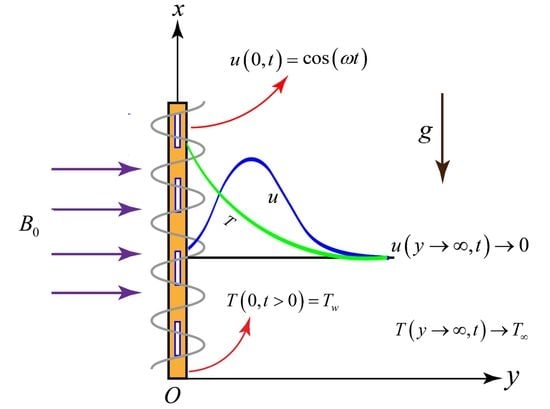
2. Mathematical Modeling of Thermoelectric Fluid

Assume a thermoelectric fluid with incompressible and unsteady flow lying above the surface of $xz -$ plane which fills the non-conducting half-space $y>0$. At the initial stage of fluid and plate, both fluid and plate are considered at rest. When $t=0^{+}$, the plate has oscillating velocity with sinusoidal variable form $u\left(0,t\right)={ℛ}_{0}sin\left(\omega t\right)$ entirely in the $x$ direction. A magnetic field of strength $H_0$ is invoked constantly in the vertical direction. Due to the motion of the fluid, an electric current is induced that is caused by the buoyancy forces, which does not distort the applied magnetic field, where $T_{\infty }$ is the temperature of the fluid and $T_w$ is the temperature of the plate away from the plate. Here, the reference temperature is considered as $T_0=T_w-T_{\infty }$, where the Thomson relation at room temperature is ${\pi }_0=T_0{k}_0$, where ${\pi }_0$ denotes the Peltier coefficient and $k_0$ represents the Seebeck coefficient. Under these assumptions, no flow occurs in the $y$ and $z$ directions. Taking the usual assumptions on the equation of motion with modified Ohm’s law and generalized energy equation, the governing boundary layer equations are subject to imposed appropriate initial, boundary and natural conditions when the medium is quiescent:

$$\frac{1}{\nu }\frac{\partial u}{\partial t}=\left(\frac{{\partial }^2}{\partial y^2}-\frac{B_0^2{\sigma }_0}{\rho \nu }\right)u-\frac{B_0{k}_0{\sigma }_0}{\rho \nu }\frac{\partial T}{\partial y},$$

(1)

$$\frac{\partial }{\partial t}\left(1+{\tau }_0\frac{\partial }{\partial t}\right)T=\frac{\left(k_0{\sigma }_0{\pi }_0+k\right)}{\rho C_p}\frac{{\partial }^{2}T}{\partial y^2}+\frac{B_0{\pi }_0{\sigma }_0}{\rho C_p}\frac{\partial u}{\partial y},$$

(2)

$$\begin{array}{c}u(y,0)=T(y,0)=u^{\prime }(y,0)=0\hfill \\ u(0,t)={\mathcal{R}}_0\mathit{sin}(\omega t),{\mathcal{R}}_{0}H(t)\mathit{cos}(\omega t) T(0,t)=1\hfill \\ u(\mathrm{\infty },t)=0,T(\mathrm{\infty },t)=T_{\mathrm{\infty }}\hfill \end{array}$$

(3)

By invoking the non-dimensional parameters on Equations (1) and (2) and then developing the governing partial differential equations in terms of Caputo-Fabrizio fractional operator, we arrive at:

$$P_r\frac{\partial }{\partial t}\left(1+{\lambda }_1{}^{CF}D_t^{\alpha }\right)\theta ={\lambda }_2\frac{{\partial }^2\theta }{\partial y^2}+{\lambda }_3\frac{\partial u}{\partial y},$$

(4)

$${}^{CF}D_t^{\alpha }u=\left(\frac{{\partial }^2}{\partial y^2}-M\right)u-K_0\frac{\partial \theta }{\partial y},$$

(5)

where ${}^{CF}D_t^{\alpha }u$ represents the Caputo-Fabrizio fractional operator of order $0<\alpha <1$, as published in previous literature [42,43,44,45]. The definition of the Caputo-Fabrizio fractional operator is stated as:

$${}^{CF}D_t^{\alpha }u=\frac{1}{1-\alpha }\underset{0}{\overset{t}{{\displaystyle \int }}}{u}^{\prime }\mathrm{e}\mathrm{x}\mathrm{p}\left(\frac{-\alpha \left(z-t\right)}{1-\alpha }\right)dt.$$

(6)

The normalization function for Equation (6) is $M\left(\alpha \right)=M\left(0\right)=M\left(1\right)$. Meanwhile, the parameters of the fractional partial differential equations for the temperature distribution and velocity field are described in Equation (7) as:

$$\begin{array}{c}{P}_r=\frac{C_p\mu }{k},{\lambda }_1={\tau }_0, {\lambda }_2=\left(1+Z{T}_0\right),\hfill \\ {\lambda }_3=\frac{\nu B_0{\pi }_0{\sigma }_0}{T_{0}k}, M=\frac{B_0^2\nu {\sigma }_0}{{ℛ}_0^2\rho }, K_0=\frac{T_0{B}_0{k}_0{\sigma }_0}{{ℛ}_0^2\rho }\hfill \end{array},$$

(7)

3. Analytic Solution of the Problem via the Caputo-Fabrizio Approach

3.1. Case-I: Sine Sinusoidal Waves $u\left(0,t\right)={ℛ}_0\mathit{sin}\left(\omega t\right)$

Applying Laplace transform [46,47] on coupled system of partial differential Equations (4) and (5), we obtain the following expression with help of Equation (3) as:

$$\left(\frac{{\partial }^2}{\partial y^2}+{\lambda }_{4}q+\frac{q^2{ϵ}_0{\lambda }_1{\lambda }_4}{\left(q+{ϵ}_0\alpha \right)}\right)\overline{\theta }={\lambda }_5\frac{\partial \overline{u}}{\partial y},$$

(8)

$$\left(\frac{{\partial }^2}{\partial y^2}-\frac{q{ϵ}_0}{q+{ϵ}_0\alpha }-M\right)\overline{u }=K_0\frac{\partial \overline{\theta }}{\partial y},$$

(9)

where ${ϵ}_0=\frac{1}{1-\alpha }$,${\lambda }_4=\frac{P_r}{{\lambda }_3}$, and ${\lambda }_5=\frac{{\lambda }_3}{{\lambda }_2}$. In order to eliminate $\overline{\theta }$ from Equations (8) and (9), by solving both equations simultaneously, we obtain:

$$\frac{{\partial }^4\overline{u}}{\partial y^4}\left({\alpha }_1+{\alpha }_2+{\alpha }_3\right)+\frac{{\partial }^2\overline{u}}{\partial y^2}\left({\beta }_1+{\beta }_2+{\beta }_3+{\beta }_4\right)-\left({\gamma }_1+{\gamma }_2+{\gamma }_3\right)=0,$$

(10)

Now, defining the letting parameters involved in Equation (10) as below:

$$\begin{array}{c}{\alpha }_1=q^2,{\alpha }_2=2{ϵ}_0\alpha q,{\alpha }_3={ϵ}_0^2{\alpha }^2,{\beta }_1=q^3\left({\lambda }_1{\lambda }_4{ϵ}_0\right),{\beta }_2=q^2\left({\lambda }_4+{\lambda }_1{\lambda }_4{ϵ}_0^2\alpha -M-{ϵ}_0\right),\hfill \\ {\beta }_3=q\left({\lambda }_4{ϵ}_0\alpha -2M{ϵ}_0\alpha -{ϵ}_0^2\alpha \right),{\beta }_4={ϵ}_0^2{\alpha }^{2}M,{\mathrm{\gamma }}_1=q^3\left(M{\lambda }_4+M{\lambda }_1{\lambda }_4{ϵ}_0+{\lambda }_4{ϵ}_0+{ϵ}_0^2{\lambda }_1{\lambda }_4\right),\hfill \\ {\mathrm{\gamma }}_2=q^2\left(M{\lambda }_1{\lambda }_4{ϵ}_0^2\alpha +{\lambda }_4{ϵ}_0^2\alpha \right),{\mathrm{\gamma }}_3=q\left(3M{\lambda }_4{ϵ}_0\alpha \right),\hfill \end{array}$$

(11)

In order to eliminate the spatial variable involved in Equation (10), a Fourier Sine transform [48,49] is invoked with the help of Appendix A (A1)–(A3), where the final form is reduced as:

$$\begin{array}{c}\left(-{\xi }^4{\overline{u}}_s\left(\xi ,q\right)+\sqrt{\frac{2}{\pi }}\frac{{ℛ}_0 {\xi }^3\omega }{q^2+{\omega }^2}+\sqrt{\frac{2}{\pi }}\frac{{ℛ}_0 \xi {\omega }^3}{q^2+{\omega }^2}\right)\left({\alpha }_1+{\alpha }_2+{\alpha }_3\right)+(-{\xi }^2{\overline{u}}_s\left(\xi ,q\right)\hfill \\ +\sqrt{\frac{2}{\pi }}\frac{{ℛ}_0 \xi \omega }{q^2+{\omega }^2})\left({\beta }_1+{\beta }_2+{\beta }_3+{\beta }_4\right)-\left({\gamma }_1+{\gamma }_2+{\gamma }_3\right){\overline{u}}_s\left(\xi ,q\right)=0\hfill \end{array},$$

(12)

Employing Equation (11) in Equation (12) and simplifying Equation (12), we obtain the following suitable equivalent expression of velocity field as:

$$\begin{array}{c}{\overline{u}}_s(\xi ,q)=\sqrt{\frac{2}{\pi }}\frac{{\mathcal{R}}_0\omega {\xi }^{-1}}{q^2+{\omega }^2}\hfill \\ -{\mathcal{R}}_0\omega \sqrt{\frac{2}{\pi }}\frac{({\mathfrak{R}}_1{q}^3+{\mathfrak{R}}_2{q}^2+{\mathfrak{R}}_{3}q+{\mathfrak{R}}_4)+{\xi }^2(1+{\xi }^2)(1+{\omega }^2)(q^2+2\alpha \beta q+{\alpha }^2{\beta }^2)}{\xi (q^2+{\omega }^2)({\mathfrak{R}}_1{q}^3+{\mathfrak{R}}_2{q}^2+{\mathfrak{R}}_{3}q+{\mathfrak{R}}_4)},\hfill \\ -{\mathcal{R}}_0\omega {\xi }^{-1}\sqrt{\frac{2}{\pi }}\frac{({\mathfrak{R}}_5{q}^3+{\mathfrak{R}}_6{q}^2+{\mathfrak{R}}_{7}q+{\mathfrak{R}}_8)}{(q^2+{\omega }^2)({\mathfrak{R}}_1{q}^3+{\mathfrak{R}}_2{q}^2+{\mathfrak{R}}_{3}q+{\mathfrak{R}}_4)}\hfill \end{array}$$

(13)

where the letting variables of rheology for Equation (13) are defined as:

$$\begin{array}{c}{\mathfrak{R}}_1={\xi }^2{\lambda }_1{\lambda }_3\beta +M{\lambda }_3+M{\lambda }_1{\lambda }_3\beta +{\lambda }_3\beta +{\beta }^2{\lambda }_1{\lambda }_2,\hfill \\ {\mathfrak{R}}_2={\xi }^4+{\xi }^2{\lambda }_3+{\xi }^2{\lambda }_1{\lambda }_3\alpha {\beta }^2-M{\xi }^2-{\xi }^2\beta +M{\lambda }_1{\lambda }_3\alpha {\beta }^2+{\lambda }_3\alpha {\beta }^2\hfill \\ {\mathfrak{R}}_3=2{\xi }^4\alpha \beta +{\xi }^2{\lambda }_3\alpha \beta -2M{\xi }^2\alpha \beta -{\xi }^2\alpha {\beta }^2+3M{\lambda }_3\alpha \beta ,\hfill \\ {\mathfrak{R}}_4={\xi }^4{\alpha }^2{\beta }^2-M{\xi }^2{\alpha }^2{\beta }^2,\hfill \\ {\mathfrak{R}}_5={\lambda }_1{\lambda }_3\beta ,\hfill \\ {\mathfrak{R}}_6={\lambda }_3+{\lambda }_1{\lambda }_3\alpha {\beta }^2-M-\beta ,\hfill \\ {\mathfrak{R}}_7={\lambda }_3\alpha \beta -2\alpha \beta M-\alpha {\beta }^2,\hfill \\ {\mathfrak{R}}_8={\alpha }^2{\beta }^{2}M,\hfill \end{array}$$

(14)

Inverting Equation (13) [5,50] by means of Fourier sine transform and invoking the fact of integral as per condition of $y>0$, the integral ${{\displaystyle \int }}_0^{\infty }\frac{\mathit{sin}\left(y\xi \right)}{\xi }d\xi =\frac{\pi }{2}$ is employed for the verification of imposed conditions on velocity field; thus, we obtain:

$$\begin{array}{c}{\overline{u}}_s(y,q)=\frac{{\mathcal{R}}_0\omega }{q^2+{\omega }^2}-\frac{2{\mathcal{R}}_0\omega }{\pi }\underset{0}{\overset{\infty }{{\displaystyle \int }}}\mathit{sin}(y\xi )\frac{\left({\mathfrak{R}}_1{q}^3+{\mathfrak{R}}_9{q}^2+{\mathfrak{R}}_{10}q+{\mathfrak{R}}_{11}\right)}{\xi \left(q^2+{\omega }^2\right)\left({\mathfrak{R}}_1{q}^3+{\mathfrak{R}}_2{q}^2+{\mathfrak{R}}_{3}q+{\mathfrak{R}}_4\right)}d\xi \hfill \\ -\frac{2{\mathcal{R}}_0\omega {\xi }^{-1}}{\pi }\underset{0}{\overset{\infty }{{\displaystyle \int }}}\mathit{sin}(y\xi )\frac{\left({\mathfrak{R}}_5{q}^3+{\mathfrak{R}}_6{q}^2+{\mathfrak{R}}_{7}q+{\mathfrak{R}}_8\right)}{\left(q^2+{\omega }^2\right)\left({\mathfrak{R}}_1{q}^3+{\mathfrak{R}}_2{q}^2+{\mathfrak{R}}_{3}q+{\mathfrak{R}}_4\right)}d\xi \hfill \end{array},$$

(15)

To simplify Equation (15), the mathematical assumptions are taken as in Equation (16):

$$\begin{array}{c}{\mathfrak{R}}_9={\mathfrak{R}}_2+{\xi }^2\left(1+{\xi }^2\right)\left(1+{\omega }^2\right),{\mathfrak{R}}_{10}={\mathfrak{R}}_3+{\xi }^2\left(1+{\xi }^2\right)\left(1+{\omega }^2\right)\alpha \beta \hfill \\ {\mathfrak{R}}_{11}={\mathfrak{R}}_4+{\xi }^2\left(1+{\xi }^2\right)\left(1+{\omega }^2\right){\alpha }^2{\beta }^2\hfill \end{array},$$

(16)

$$\begin{array}{c}{\overline{u}}_s(y,q)=\frac{{\mathcal{R}}_0\omega }{q^2+{\omega }^2}-\frac{2{\mathcal{R}}_0\omega }{\pi }\underset{0}{\overset{\infty }{{\displaystyle \int }}}sin(y\xi )\frac{\left(q^3+{\mathfrak{R}}_{12}{q}^2+{\mathfrak{R}}_{13}q+{\mathfrak{R}}_{14}\right)}{\xi \left(q^2+{\omega }^2\right)\left(q^3+{\mathfrak{R}}_{15}{q}^2+{\mathfrak{R}}_{16}q+{\mathfrak{R}}_{17}\right)}d\xi \hfill \\ -\frac{2{\mathfrak{R}}_5{\mathcal{R}}_0\omega {\xi }^{-1}}{{\mathfrak{R}}_1\pi }\underset{0}{\overset{\infty }{{\displaystyle \int }}}\mathit{sin}(y\xi )\frac{\left(q^3+{\mathfrak{R}}_{18}{q}^2+{\mathfrak{R}}_{19}q+{\mathfrak{R}}_{20}\right)}{\left(q^2+{\omega }^2\right)\left(q^3+{\mathfrak{R}}_{15}{q}^2+{\mathfrak{R}}_{16}q+{\mathfrak{R}}_{17}\right)}d\xi \hfill \end{array},$$

(17)

where the letting parameters are taken as: ${\mathfrak{R}}_{12}=\frac{{\mathfrak{R}}_9}{{\mathfrak{R}}_1}, {\mathfrak{R}}_{13}=\frac{{\mathfrak{R}}_{10}}{{\mathfrak{R}}_1}, {\mathfrak{R}}_{14}=\frac{{\mathfrak{R}}_{11}}{{\mathfrak{R}}_1}, {\mathfrak{R}}_{15}=\frac{{\mathfrak{R}}_2}{{\mathfrak{R}}_1}, {\mathfrak{R}}_{16}=\frac{{\mathfrak{R}}_3}{{\mathfrak{R}}_1}, {\mathfrak{R}}_{17}=\frac{{\mathfrak{R}}_4}{{\mathfrak{R}}_1}, {\mathfrak{R}}_{18}=\frac{{\mathfrak{R}}_6}{{\mathfrak{R}}_5}, {\mathfrak{R}}_{19}=\frac{{\mathfrak{R}}_7}{{\mathfrak{R}}_5} \mathrm{and} {\mathfrak{R}}_{20}=\frac{{\mathfrak{R}}_8}{{\mathfrak{R}}_5}.$

In order avoid the lengthy and cumbersome calculation of Equation (17), the following expression is taken with the help of Cardano’s method [51], which is defined as:

$$\begin{array}{c}{q}_1=\sqrt[3]{-\frac{{\delta }_1}{2}-\sqrt{\frac{{\delta }_1^2}{4}+\frac{{\Delta }_1^3}{27}}}+\sqrt[3]{-\frac{{\delta }_1}{2}+\sqrt{\frac{{\delta }_1^2}{4}+\frac{{\Delta }_1^3}{27}}}\hfill \\ q_2=\mathsf{\gamma }\sqrt[3]{-\frac{{\delta }_1}{2}-\sqrt{\frac{{\delta }_1^2}{4}+\frac{{\Delta }_1^3}{27}}}+{\mathsf{\gamma }}^2\sqrt[3]{-\frac{{\delta }_1}{2}+\sqrt{\frac{{\delta }_1^2}{4}+\frac{{\Delta }_1^3}{27}}},\hfill \\ q_3={\mathsf{\gamma }}^2\sqrt[3]{-\frac{{\delta }_1}{2}-\sqrt{\frac{{\delta }_1^2}{4}+\frac{{\Delta }_1^3}{27}}}+\mathsf{\gamma }\sqrt[3]{-\frac{{\delta }_1}{2}+\sqrt{\frac{{\delta }_1^2}{4}+\frac{{\Delta }_1^3}{27}}}\hfill \end{array}$$

(18)

where $q_1,q_2$ and $q_3$ are the roots of an algebraic cubic equation. The roots of an algebraic cubic equation are obtained in Equation (19) by using Cardano’s formulae as:

$$\left(q^3+{\mathfrak{R}}_{15}{q}^2+{\mathfrak{R}}_{16}q+{\mathfrak{R}}_{17}\right)=\left(q-q_1\right)\left(q-q_2\right)\left(q-q_3\right),$$

(19)

Solving Equation (17) in its simplest form with the help of Equation (19), we arrive at:

$$\begin{array}{c}{\overline{u}}_s(y,q)=\frac{{\mathcal{R}}_0\omega }{q^2+{\omega }^2}-\frac{2{\mathcal{R}}_0\omega }{\pi }\underset{0}{\overset{\infty }{{\displaystyle \int }}}{\xi }^{-1}sin(y\xi )\frac{\left(q^3+{\mathfrak{R}}_{12}{q}^2+{\mathfrak{R}}_{13}q+{\mathfrak{R}}_{14}\right)}{\left(q^2+{\omega }^2\right)\left(q-q_1\right)\left(q-q_2\right)\left(q-q_3\right)}d\xi \hfill \\ -\frac{2{\mathfrak{R}}_5{\mathcal{R}}_0\omega {\xi }^{-1}}{{\mathfrak{R}}_1\pi }\underset{0}{\overset{\infty }{{\displaystyle \int }}}\mathit{sin}(y\xi )\frac{\left(q^3+{\mathfrak{R}}_{18}{q}^2+{\mathfrak{R}}_{19}q+{\mathfrak{R}}_{20}\right)}{\left(q^2+{\omega }^2\right)\left(q-q_1\right)\left(q-q_2\right)\left(q-q_3\right)}d\xi \hfill \end{array},$$

(20)

Invoking Appendix A (A4) with inverse Laplace transform on Equation (20), we obtain the expression of velocity via the exponential elementary functions as:

$$\begin{array}{c}u(y,t)={\mathcal{R}}_0\mathit{sin}(\omega t)-\frac{2U\omega }{\pi }\underset{0}{\overset{\infty }{{\displaystyle \int }}}{\xi }^{-1}\mathit{sin}(y\xi )\underset{t}{\overset{t}{{\displaystyle \int }}}\mathit{cos}\omega (t-\epsilon )\left\{\frac{{\mathfrak{R}}_{14}}{q_1{q}_2{q}_3}-\left(\frac{{\mathfrak{R}}_{14}-q_1{\mathfrak{R}}_{13}+q_1^2{\mathfrak{R}}_{12}-q_1^2}{q_1\left(q_2-q_1\right)\left(q_3-q_1\right)}\right)\right.\hfill \\ \left.\times \exp \left(-q_{1}t\right)-\left(\frac{{\mathfrak{R}}_{14}-q_2{\mathfrak{R}}_{13}+q_2^2{\mathfrak{R}}_{12}-q_2^3}{q_2\left(q_1-q_2\right)\left(q_3-q_2\right)}\right)\exp \left(-q_{2}t\right)-\left(\frac{{\mathfrak{R}}_{14}-q_3{\mathfrak{R}}_{13}+q_3^2{\mathfrak{R}}_{12}-q_3^3}{q_3\left(q_1-q_3\right)\left(q_2-q_3\right)}\right)\exp \left(-q_{3}t\right)\right\}d\xi d\epsilon \hfill \\ -\frac{2{\mathfrak{R}}_{5}U\omega {\xi }^{-1}}{{\mathfrak{R}}_1\pi }\underset{0}{\overset{\infty }{{\displaystyle \int }}}\mathit{sin}(y\xi )\underset{t}{\overset{t}{{\displaystyle \int }}}\mathit{cos}\omega (t-\epsilon )\left\{\frac{{\mathfrak{R}}_{14}}{q_1{q}_2{q}_3}-\left(\frac{{\mathfrak{R}}_{20}-q_1{\mathfrak{R}}_{19}+q_1^2{\mathfrak{R}}_{18}-q_1^2}{q_1\left(q_2-q_1\right)\left(q_3-q_1\right)}\right)\exp \left(-q_{1}t\right)\right.\hfill \\ \left.-\left(\frac{{\mathfrak{R}}_{20}-q_2{\mathfrak{R}}_{19}+q_2^2{\mathfrak{R}}_{18}-q_2^3}{q_2\left(q_1-q_2\right)\left(q_3-q_2\right)}\right)\exp \left(-q_{2}t\right)-\left(\frac{{\mathfrak{R}}_{20}-q_3{\mathfrak{R}}_{19}+q_3^2{\mathfrak{R}}_{18}-q_3^3}{q_3\left(q_1-q_3\right)\left(q_2-q_3\right)}\right)\exp \left(-q_{3}t\right)\right\}d\xi d\epsilon .\hfill \end{array}$$

(21)

Equation (20) is the general solution for the velocity field based on the fractional approaches of Caputo-Fabrizio for sine sinusoidal waves; it also validates the imposed initial and boundary conditions.

3.2. Case-II: Cosine Sinusoidal Waves $u\left(0,t\right)={ℛ}_{0}H\left(t\right)\mathit{cos}\left(\omega t\right)$

In order to avoid lengthy and cumbersome calculation, the solution for the velocity field of the cosine sinusoidal waves has been investigated by employing similar procedure as discussed in case-I:

$$\begin{array}{c}u(y,t)={\mathcal{R}}_{0}H(t)\mathit{cos}(\omega t)-\frac{2U\omega }{\pi }\underset{0}{\overset{\infty }{{\displaystyle \int }}}{\xi }^{-1}\mathit{sin}(y\xi )\underset{t}{\overset{t}{{\displaystyle \int }}}\mathit{sin}\omega (t-\epsilon )\left\{\frac{{\mathfrak{R}}_{14}}{q_1{q}_2{q}_3}-\left(\frac{{\mathfrak{R}}_{14}-q_1{\mathfrak{R}}_{13}+q_1^2{\mathfrak{R}}_{12}-q_1^2}{q_1\left(q_2-q_1\right)\left(q_3-q_1\right)}\right)\right.\hfill \\ \left.\times \exp \left(-q_{1}t\right)-\left(\frac{{\mathfrak{R}}_{14}-q_2{\mathfrak{R}}_{13}+q_2^2{\mathfrak{R}}_{12}-q_2^3}{q_2\left(q_1-q_2\right)\left(q_3-q_2\right)}\right)\exp \left(-q_{2}t\right)-\left(\frac{{\mathfrak{R}}_{14}-q_3{\mathfrak{R}}_{13}+q_3^2{\mathfrak{R}}_{12}-q_3^3}{q_3\left(q_1-q_3\right)\left(q_2-q_3\right)}\right)\exp \left(-q_{3}t\right)\right\}d\xi d\epsilon \hfill \\ -\frac{2{\mathfrak{R}}_{5}UH(t)\omega {\xi }^{-1}}{{\mathfrak{R}}_1\pi }\underset{0}{\overset{\infty }{{\displaystyle \int }}}\mathit{sin}(y\xi )\underset{t}{\overset{t}{{\displaystyle \int }}}\mathit{sin}\omega (t-\epsilon )\left\{\frac{{\mathfrak{R}}_{14}}{q_1{q}_2{q}_3}-\left(\frac{{\mathfrak{R}}_{20}-q_1{\mathfrak{R}}_{19}+q_1^2{\mathfrak{R}}_{18}-q_1^2}{q_1\left(q_2-q_1\right)\left(q_3-q_1\right)}\right)\exp \left(-q_{1}t\right)\right.\hfill \\ \left.-\left(\frac{{\mathfrak{R}}_{20}-q_2{\mathfrak{R}}_{19}+q_2^2{\mathfrak{R}}_{18}-q_2^3}{q_2\left(q_1-q_2\right)\left(q_3-q_2\right)}\right)\exp \left(-q_{2}t\right)-\left(\frac{{\mathfrak{R}}_{20}-q_3{\mathfrak{R}}_{19}+q_3^2{\mathfrak{R}}_{18}-q_3^3}{q_3\left(q_1-q_3\right)\left(q_2-q_3\right)}\right)\exp \left(-q_{3}t\right)\right\}d\xi d\epsilon .\hfill \end{array}$$

(22)

Meanwhile, the solutions investigated for both cases viz sine and cosine sinusoidal waves, can also be retrieved for ordinary/classical differential operator by letting the fractional parameter equal the one in Equations (21) and (22). Additionally, similar solutions can be investigated in light of [52,53,54,55,56].

4. Parametric Results

The mathematical analysis of thermoelectricity has been constructed with a newly presented fractional approach of Caputo-Fabrizio based on a non-singular kernel. The main contribution is to investigate the analytical solutions of velocity field based on fractional and non-fractional approaches. The general solutions have been established through Fourier sine and Laplace transform by setting suitable imposed conditions. The Cardano’s method for the simplifications of lengthy and cumbersome mathematical expressions is employed. However, the dynamics and synchronization of the problem is listed as:

(i)

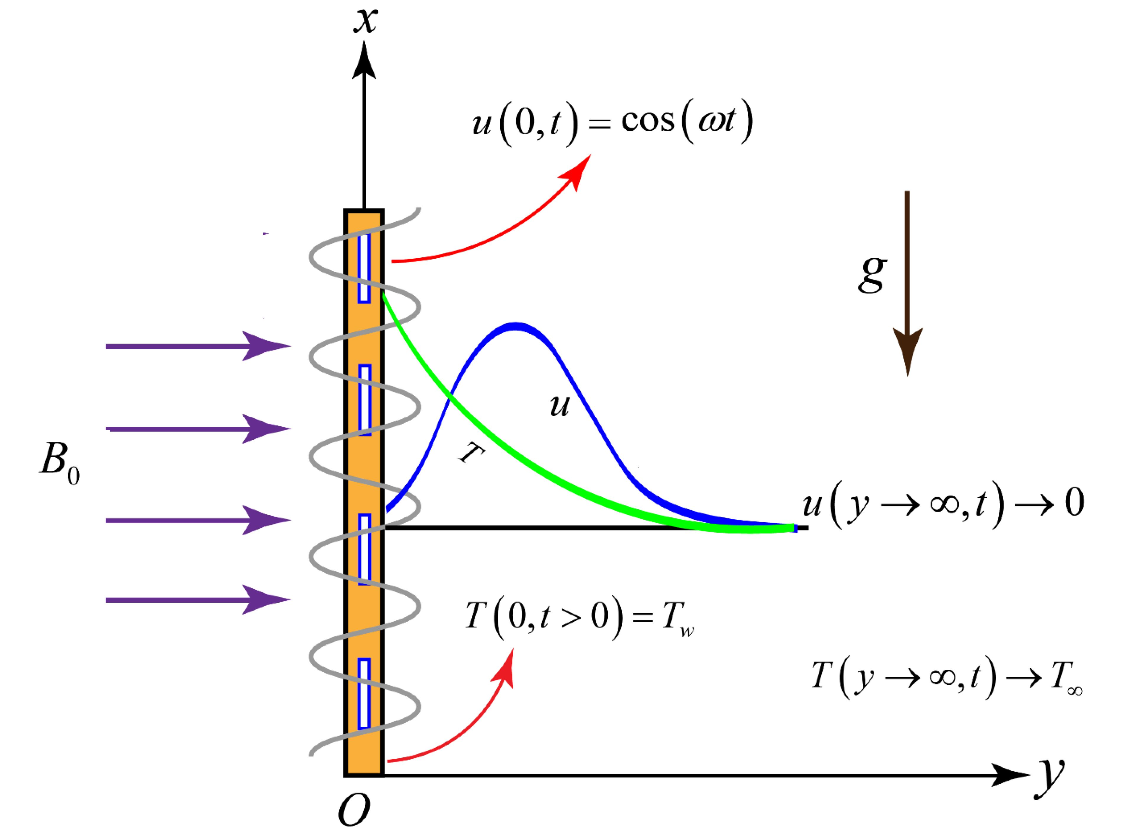
Figure 1 is prepared for the time analysis of velocity field based on thermoelectric effects. Here, the velocity field is profiled for three different increasing times $t=2 \mathrm{s}, 4 \mathrm{s}, 6 \mathrm{s}$. It is observed that thermoelectric conversion efficiency is increasing as time increases. From a physical point of view, enhancing the behavior of the thermoelectric effect leads to a temperature gradient in the heat flow. Additionally, the bar graph is sketched in Figure 1, reflecting the similar stability of thermoelectric efficiency as time increases. Furthermore, a good thermal insulator provides good thermal insulation to the industrial processes during material manufacturing.

(ii)

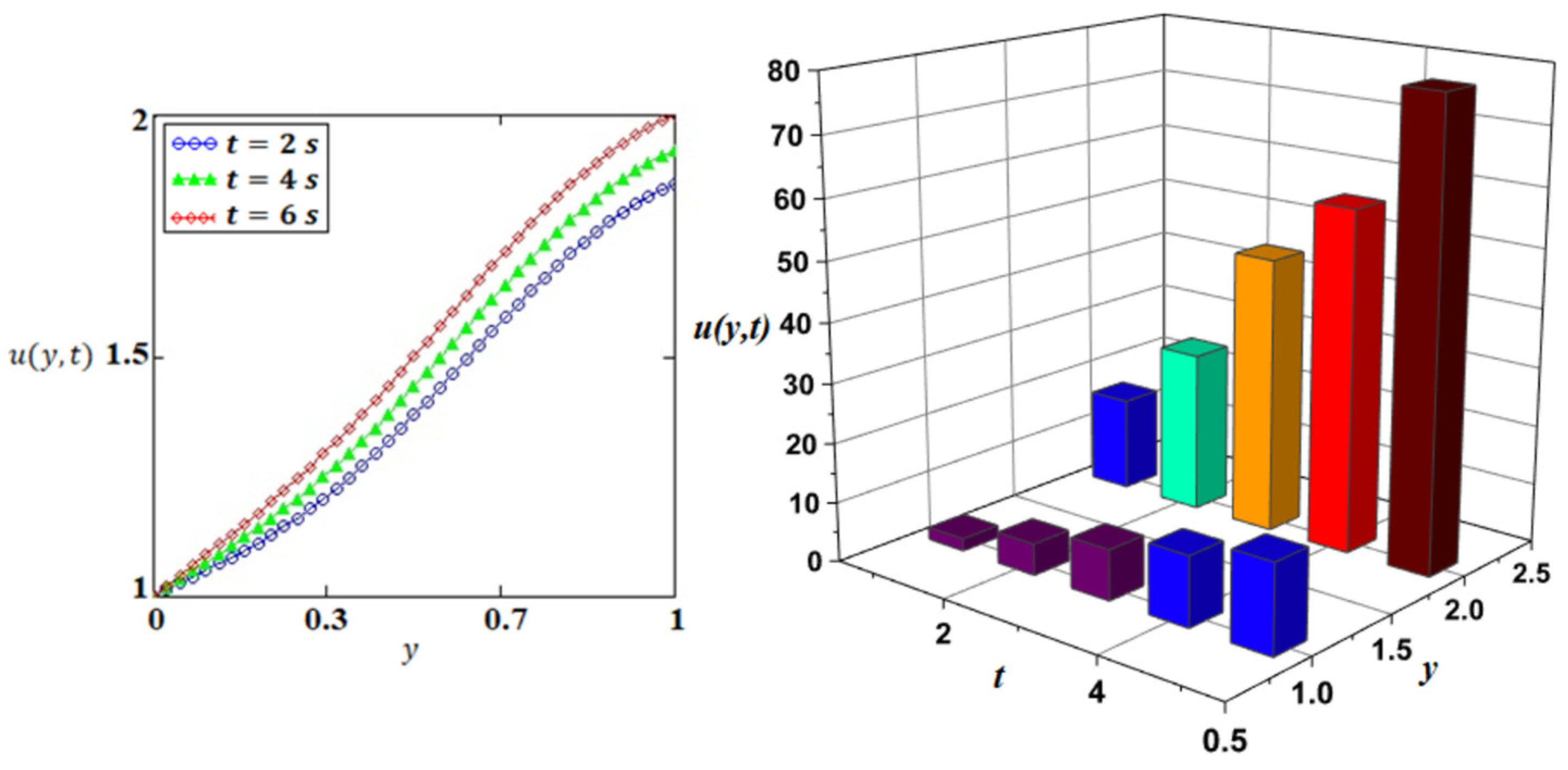
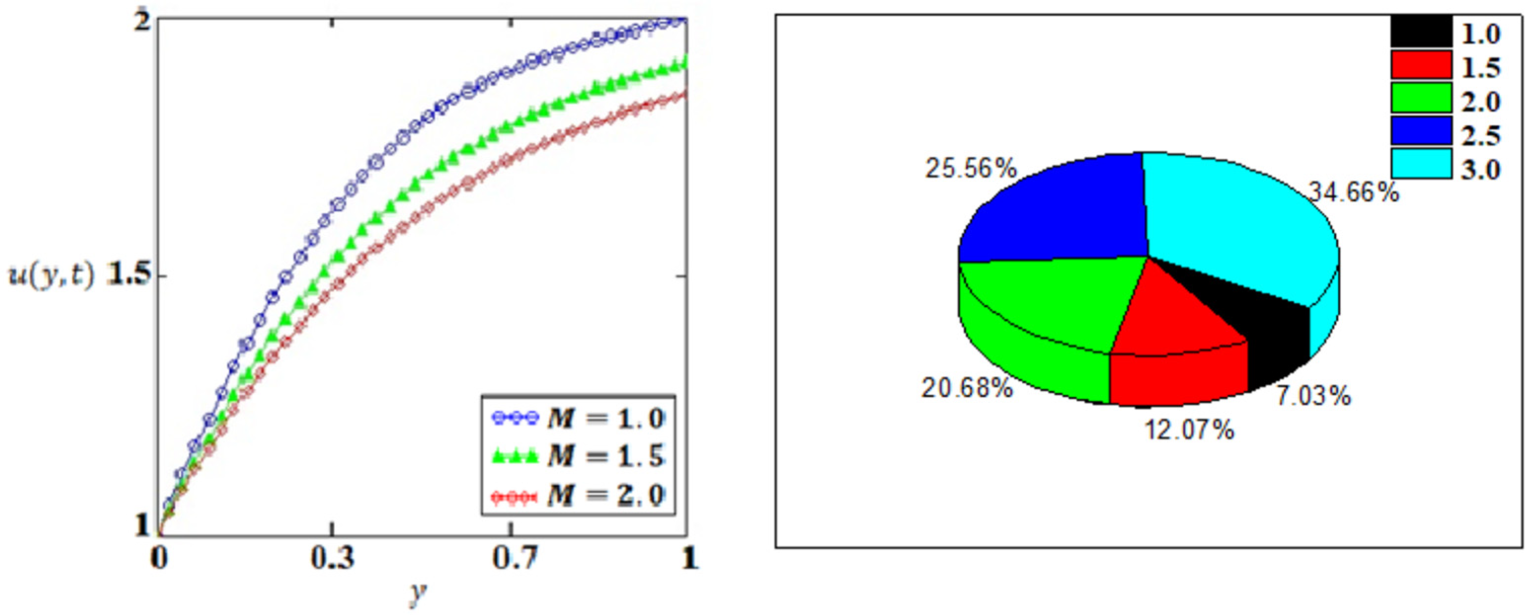
It is a well-noted statement that thermoelectric effects depend on the relative alignment of the magnetization. The effects of a magnetic field on the velocity field are depicted in Figure 2. It is noted from the behavior depicted in Figure 2 that a mosaic magnetic-domain structure is achieved through increasing effects of the magnetic field. From a practical approach, a velocity field vividly reduces when the magnetic field parameter is increased; this is due to the fact that a magnetic field depends upon the Lorenz force, which leads to the resistivity and retardation of thermoelectric fluid flow.

(iii)

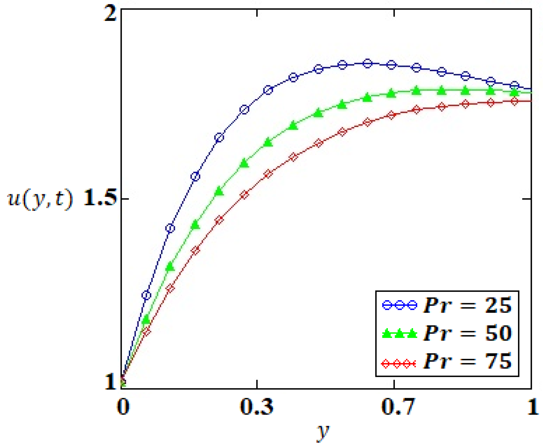
The characterization of convection is usually based on the Prandtl number, in which momentum diffusivity can be achieved by supplying larger values of the Prandtl number, while thermal diffusivity is perceived when smaller values of the Prandtl number are employed. In this analysis, the temperature and velocity field are coupled, so three different larger values of $Pr=25, 50, 75$ are utilized in Figure 3 for the thermoelectric fluid flow. Practically, higher heat transfer of thermoelectric fluid can be detected by supplying a lower Prandtl number; hence, we utilized a larger Prandtl number for obtaining the suitable velocity profile based on momentum diffusivity. It should be noted that most of the common thermoelectric fluids, $Pr \mathrm{of} \mathrm{water}=1 \mathrm{to} 10$, $Pr \mathrm{of} \mathrm{ethylene} \mathrm{glycol}=2 \mathrm{to} 30$, $Pr \mathrm{of} \mathrm{engine} \mathrm{oil}=50 \mathrm{to} 2000$, have certain physical aspects due to their larger Prandtl number.

(iv)

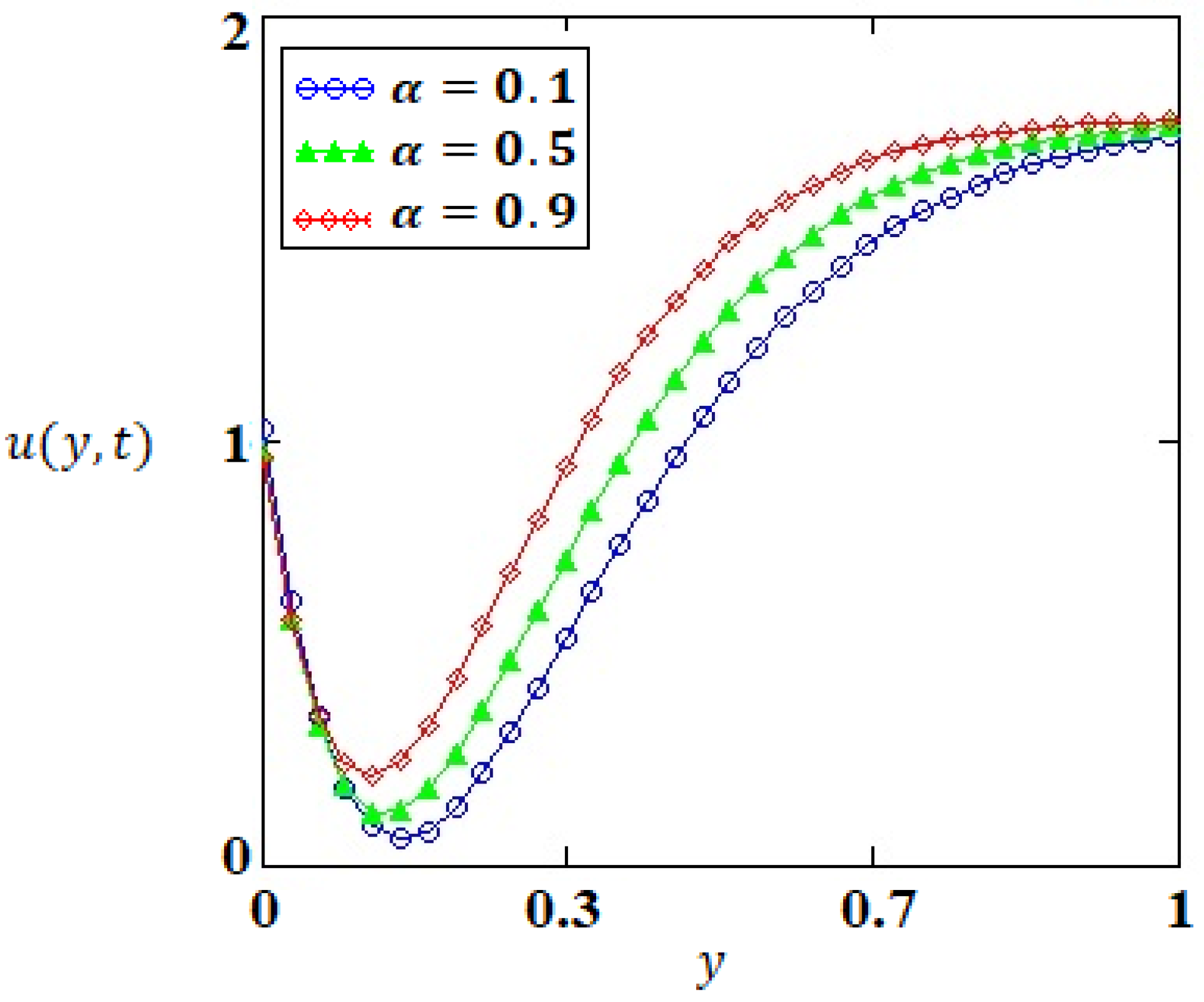
Figure 4 elucidates the dynamics of the fractional operator of Caputo-Fabrizio on the profile of the velocity field. It is clear from Figure 4 that the velocity field shows asymptotic exponential decay behavior, which is due to the Caputo-Fabrizio operator having a non-singular exponential kernel. The possibility of a memory effect needs to be considered, as when the value of the fractional derivative is closer to the classical derivative, it has an increasing trend or velocity field.

(v)

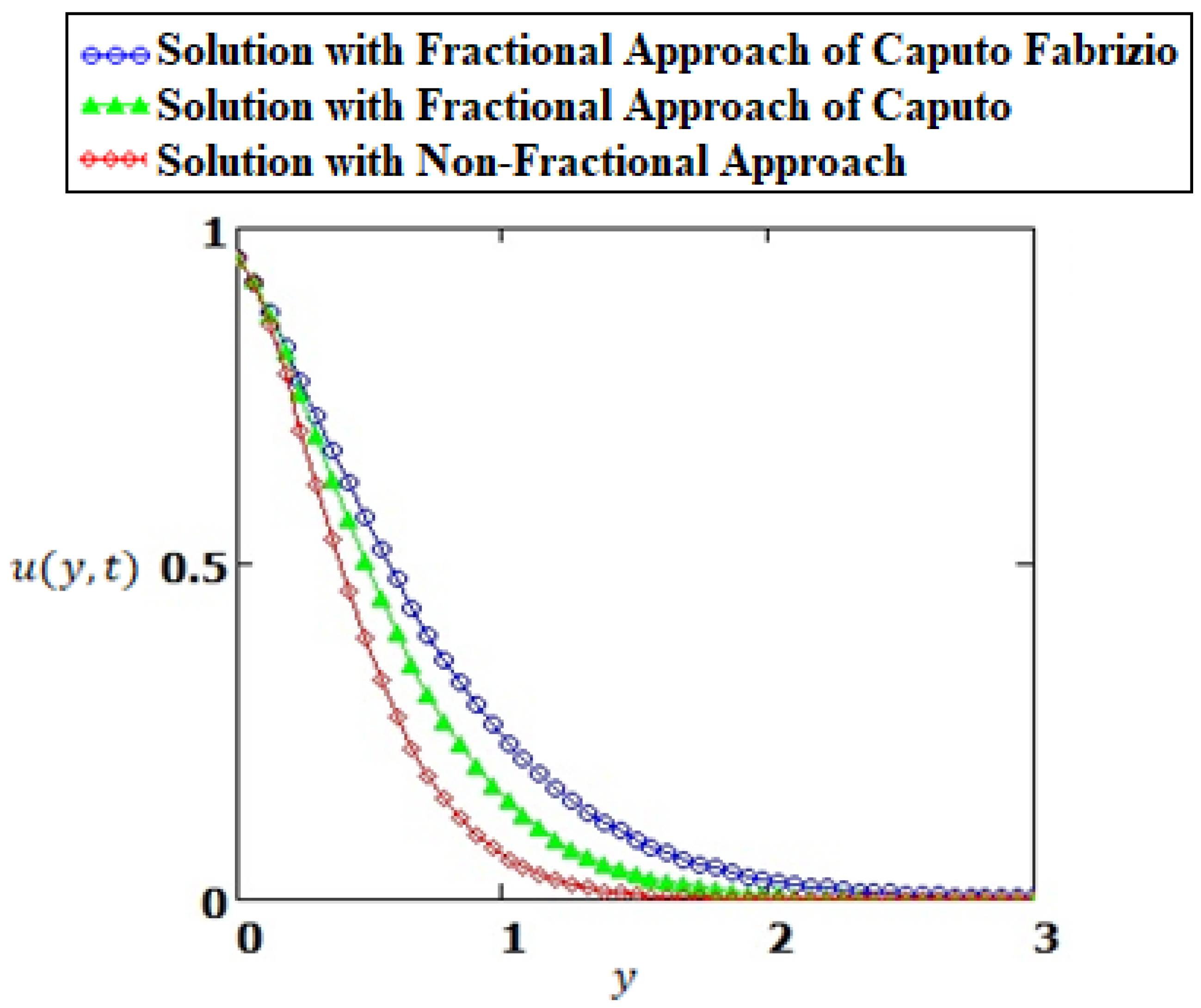
The comparative analysis is based on three types of approaches, namely (i) solution with fractional approach of Caputo-Fabrizio, (ii) solution with published approach [5] (Caputo fractional operator) and (iii) solution with non-fractional approach (ordinary operator). It can be seen from Figure 5 that the solution with the fractional approach of Caputo-Fabrizio has a greater stability and accuracy in comparison with the solution in [5] (Caputo fractional operator) and the solution with a non-fractional approach (ordinary operator). This may be due to fact that the fractional approach of Caputo-Fabrizio is based on the non-singular and exponential kernel, which describes the dynamics and other characteristic of hereditary thermoelectric materials in better ways.

5. Conclusions

This study demonstrated thermoelectric conversion efficiency via magnetization, which provides a promising path to transfer continuous and uninterrupted heat. A mathematical model based on thermoelectric effect is developed for the thermal analysis of fluid flow that captured the rheological behavior through the local kernel approach. The major findings can be summarized as follows:

-

Enhancing the thermoelectric effect for three different increasing times, $t=2 \mathrm{s}, 4 \mathrm{s}, 6 \mathrm{s}$, leads to a temperature gradient in the heat flow. This is because the thermoelectric conversion efficiency increases as time increases.

-

The effects of the magnetic field and mosaic magnetic-domain structure are achieved by increasing the effects of the magnetic field on the velocity field.

-

The temperature and velocity field are coupled for three different Prandtl values, $Pr=25, 50, 75$, where a higher heat transfer of thermoelectric fluid is detected for a lower Prandtl number.

-

The dynamics of the fractional operator of Caputo-Fabrizio on the velocity field display asymptotic exponential decay.

-

The comparative analysis suggests that the velocity and temperature distribution with the fractional approach of Caputo-Fabrizio has a greater stability and accuracy in comparison with other solutions.

References

1. Riffat, S.; Ma, X. Thermoelectric: A review of present and potential applications. Appl. Therm. Eng. 2003, 23, 913–935. [Google Scholar] [CrossRef]
2. Chein, R.; Hung, G. Thermoelectric cooler application in electronic cooling. Appl. Therm. Eng. 2004, 24, 2207–2217. [Google Scholar] [CrossRef]
3. Zhang, H.; Mui, Y.; Tarin, M. Analysis of thermoelectric cooler performance for high power electronic packages. Appl. Therm. Eng. 2010, 30, 561–568. [Google Scholar] [CrossRef]
4. Abro, K.A.; Shaikh, H.S.; Khan, I. A mathematical Study of Magnetohydrodynamic Casson Fluid via Special Functions with Heat and Mass Transfer embedded in Porous Plate. arXiv 2017, arXiv:1706.03829. [Google Scholar]
5. Ezzat, M.A. Theory of fractional order in generalized thermoelectric MHD. Appl. Math. Model. 2011, 35, 4965–4978. [Google Scholar] [CrossRef]
6. Wiriyasart, S.; Naphon, P.; Hommalee, C. Sensible air cool-warm fan with thermoelectric module systems Development. Case Stud. Therm. Eng. 2019, 13, 100369. [Google Scholar] [CrossRef]
7. He, W.; Zhou, J.; Hou, J.; Chen, C.; Ji, J. Theoretical and experimental investigation on a thermoelectric cooling and heating system driven by solar. Appl. Energy 2013, 107, 89–97. [Google Scholar] [CrossRef]
8. Abro, K.A.; Qureshi, S.; Atangana, A. Mathematical and numerical optimality of non-singular fractional approaches on free and forced linear oscillator. Nonlinear Eng. 2020, 9, 449–456. [Google Scholar] [CrossRef]
9. Martínez, A.; Astrain, D.; Rodríguez, A. Dynamic model for simulation of thermoelectric self cooling applications. Energy 2013, 55, 1114–1126. [Google Scholar] [CrossRef]
10. Abro, K.A. Numerical study and chaotic oscillations for aerodynamic model of wind turbine via fractal and fractional differential operators. Numer. Methods Partial. Differ. Equ. 2020, 14, 1–15. [Google Scholar] [CrossRef]
11. Liu, Z.; Zhang, L.; Gong, G. Experimental evaluation of a solar thermoelectric cooled ceiling combined with displacement ventilation system. Energy Convers. Manag. 2014, 87, 559–565. [Google Scholar] [CrossRef]
12. Abro, K.A.; Khan, I. Analysis of Heat and Mass Transfer in MHD Flow of Generalized Casson Fluid in a Porous Space Via Non-Integer Order Derivative without Singular Kernel. Chin. J. Phys. 2017, 55, 1583–1595. [Google Scholar] [CrossRef]
13. Zhao, D.; Tan, G. Experimental evaluation of a prototype thermoelectric system integrated with PCM (phase change material) for space cooling. Energy 2014, 68, 658–666. [Google Scholar] [CrossRef]
14. Khan, A.; Abro, K.A.; Tassaddiq, A.; Khan, I. Atangana-Baleanu and Caputo Fabrizio Analysis of Fractional Derivatives for Heat and Mass Transfer of Second Grade Fluids over a Vertical Plate: A Comparative study. Entropy 2017, 19, 279. [Google Scholar] [CrossRef] [Green Version]
15. Abro, K.A.; Hussain, M.; Baig, M.M. An Analytic Study of Molybdenum Disulfide Nanofluids Using Modern Approach of Atangana-Baleanu Fractional Derivatives, European Physical Journal Plus. Eur. Phys. J. Plus 2017, 132, 439. [Google Scholar] [CrossRef]
16. Hristov, J. Space-fractional diffusion with a potential power-law coefficient: Transient approximate solution. Prog. Fract. Differ. Appl. 2017, 3, 19–39. [Google Scholar] [CrossRef]
17. Owolabi, K.M.; Gomez-Aguilar, J.F. Numerical simulations of multilingual competition dynamics with nonlocal derivative. Chaos Solitons Fractals 2018, 117, 175–182. [Google Scholar] [CrossRef]
18. Khader, M.M.; Saad, K.M. On the numerical evaluation for studying the fractional KdV, KdV-Burgers and Burgers equations. Eur. Phys. J. Plus 2018, 133, 3335. [Google Scholar] [CrossRef]
19. Saad, K.M.; L-Sharif, E.H.F.A. Comparative study of a cubic autocatalytic reaction via different analysis methods. Discret. Contin. Dyn. Syst. 2019, 12, 665–684. [Google Scholar]
20. Almani, S.; Qureshi, K.; Abro, K.A.; Abro, M.; Unar, I.N. Parametric study of adsorption column for arsenic removal on the basis of numerical simulations. Waves Random Complex Media 2022, 1–17. [Google Scholar] [CrossRef]
21. Khader, M.M.; Saad, K.M. A numerical approach for solving the problem of biological invasion (fractional Fisher equation) using Chebyshev spectral collocation method. Chaos Solitons Fractals 2018, 110, 169–177. [Google Scholar] [CrossRef]
22. Hussain, T.; Awan, A.U.; Abro, K.A.; Ozair, M.; Manzoor, M. A mathematical and parametric study of epidemiological smoking model: A deterministic stability and optimality for solutions. Eur. Phys. J. Plus 2021, 136, 11. [Google Scholar] [CrossRef]
23. Atangana, A.; Nieto, J.J. Numerical solution for the model of RLC circuit via the fractional derivative without singular kernel. Adv. Mech. Eng. 2015, 7, 1–7. [Google Scholar] [CrossRef]
24. Abro, K.A.; Atangana, A. Numerical and mathematical analysis of induction motor by means of AB-fractal–fractional differentiation actuated by drilling system. Numer. Methods Partial. Differ. Equ. 2020, 38, 1–15. [Google Scholar] [CrossRef]
25. Abro, K.A.; Atangana, A.; Gómez-Aguilar, J. Chaos control and characterization of brushless DC motor via integral and differential fractal-fractional techniques. Int. J. Model. Simul. 2022, 1–10. [Google Scholar] [CrossRef]
26. Sheikh, N.A.; Ali, F.; Khan, I.; Gohar, M.; Saqib, M. On the applications of nanofluids to enhance the performance of solar collectors: A comparative analysis of Atangana-Baleanu and Caputo-Fabrizio fractional models. Eur. Phys. J. Plus 2017, 132, 540. [Google Scholar] [CrossRef]
27. Abro, K.A. Fractional characterization of fluid and synergistic effects of free convective flow in circular pipe through Hankel transform. Phys. Fluids 2020, 32, 123102. [Google Scholar] [CrossRef]
28. Abro, K.A.; Memon, I.Q.; Siyal, A. Thermal transmittance and thermo-magnetization of unsteady free convection viscous fluid through non-singular differentiations. Phys. Scr. 2020, 96, 015215. [Google Scholar] [CrossRef]
29. Ali, F.; Alam Jan, S.A.; Khan, I.; Gohar, M.; Sheikh, N.A. Solutions with special functions for time fractional free convection flow of Brinkman-type fluid. Eur. Phys. J. Plus 2016, 131, 310. [Google Scholar] [CrossRef]
30. Souayeh, B.; Abro, K.A.; Siyal, A.; Hdhiri, N.; Hammami, F.; Al-Shaeli, M.; Alnaim, N.; Raju, S.S.K.; Alam, M.W.; Alsheddi, T. Role of copper and alumina for heat transfer in hybrid nanofluid by using Fourier sine transform. Sci. Rep. 2022, 12, 11307. [Google Scholar] [CrossRef]
31. Memon, I.Q.; Abro, K.A.; Solangi, M.A.; Shaikh, A.A. Functional shape effects of nanoparticles on nanofluid suspended in ethylene glycol through Mittage-Leffler approach. Phys. Scr. 2020, 96, 025005. [Google Scholar] [CrossRef]
32. Abro, K.A.; Siyal, A.; Souayeh, B.; Atangana, A. Application of Statistical Method on Thermal Resistance and Conductance during Magnetization of Fractionalized Free Convection Flow. Int. Commun. Heat Mass Transf. 2020, 119, 104971. [Google Scholar] [CrossRef]
33. Abro, K.A.; Soomro, M.; Atangana, A.; Gómez-Aguilar, J.F. Thermophysical properties of Maxwell Nanoluids via fractional derivatives with regular kernel. J. Therm. Anal. Calorim. 2020, 147, 449–459. [Google Scholar] [CrossRef]
34. Gómez-Aguilar, J.; Yépez-Martínez, H.; Escobar-Jiménez, R.; Astorga-Zaragoza, C.; Reyes-Reyes, J. Analytical and numerical solutions of electrical circuits described by fractional derivatives. Appl. Math. Model. 2016, 40, 9079–9094. [Google Scholar] [CrossRef]
35. Lohana, B.; Abro, K.A.; Shaikh, A.W. Thermodynamical analysis of heat transfer of gravity-driven fluid flow via fractional treatment: An analytical study. J. Therm. Anal. Calorim. 2020, 144, 155–165. [Google Scholar] [CrossRef]
36. Morales-Delgado, V.F.; Gómez-Aguilar, J.F.; Kumar, S.; Taneco-Hernández, M.A. Analytical solutions of the Keller-Segel chemotaxis model involving fractional operators without singular kernel. Eur. Phys. J. Plus 2018, 133, 200. [Google Scholar] [CrossRef]
37. Ali, Q.; Yassen, M.F.; Asiri, S.A.; Pasha, A.A.; Abro, K.A. Role of viscoelasticity on thermo-electromechanical system subjected to annular regions of cylinders in the existence of a uniform inclined magnetic field. Eur. Phys. J. Plus 2022, 137, 770. [Google Scholar] [CrossRef]
38. Owolabi, K.M.; Atangana, A. Robustness of fractional difference schemes via the Caputo subdiffusion-reaction equations. Chaos Solitons Fractals 2018, 111, 119–127. [Google Scholar] [CrossRef]
39. Abro, K.A.; Atangana, A. Numerical study and chaotic analysis of meminductor and memcapacitor through fractal-fractional differential operator. Arab. J. Sci. Eng. 2020, 46, 857–871. [Google Scholar] [CrossRef]
40. Gómez-Aguilar, J.F.; Atangana, A. Fractional derivatives with the power-law and the Mittaga-Leffler kernel applied to the nonlinear Baggs-Freedman model. Fractal Fract. 2018, 2, 10. [Google Scholar] [CrossRef] [Green Version]
41. Panhwer, L.A.; Abro, K.A.; Memon, I.Q. Thermal deformity and thermolysis of magnetized and fractional Newtonian fluid with rheological investigation. Phys. Fluids 2022, 34, 053115. [Google Scholar] [CrossRef]
42. Caputo, M.; Fabrizio, M. A new definition of fractional derivative without singular kernel. Prog. Fract. Differ. Appl. 2015, 1, 73–85. [Google Scholar]
43. Abro, K.A.; Atangana, A.; Memon, I.Q. Comparative analysis of statistical and fractional approaches for thermal conductance through suspension of ethylene glycol nanofluid. Braz. J. Phys. 2022, 52, 118. [Google Scholar] [CrossRef]
44. Abro, K.A.; Atangana, A. Mathematical analysis of memristor through fractal-fractional differential operators: A numerical study. Math. Methods Appl. Sci. 2020, 43, 6378–6395. [Google Scholar] [CrossRef]
45. Abro, K.A.; Atangana, A. A comparative study of convective fluid motion in rotating cavity via Atangana–Baleanu and Caputo–Fabrizio fractal–fractional differentiations. Eur. Phys. J. Plus 2020, 135, 226–242. [Google Scholar] [CrossRef]
46. Abro, K.A.; Siyal, A.; Atangana, A. Thermal stratification of rotational second-grade fluid through fractional differential operators. J. Therm. Anal. 2020, 143, 3667–3676. [Google Scholar] [CrossRef]
47. Abro, K.A.; Atangana, A. Role of Non-integer and Integer Order Differentiations on the Relaxation Phenomena of Viscoelastic Fluid. Phys. Scr. 2019, 95, 035228. [Google Scholar] [CrossRef]
48. Abro, K.A. A fractional and analytic investigation of thermo-diffusion process on free convection flow: An application to surface modification technology. Eur. Phys. J. Plus 2020, 135, 31–45. [Google Scholar] [CrossRef]
49. Ezzat, M.; Sabbah, A.; El-Bary, A.; Ezzat, S.M. Stokes’ first problem for a thermoelectric fluid with fractional order heat transfer. Rep. Math. Phys. 2014, 74, 145–158. [Google Scholar] [CrossRef]
50. Souayeh, B.; Abro, K.A.; Alnaim, N.; Al Nuwairan, M.; Hdhiri, N.; Yasin, E. Heat transfer characteristics of fractionalized hydromagnetic fluid with chemical reaction in permeable media. Energies 2022, 15, 2196. [Google Scholar] [CrossRef]
51. Kuros, A. Cours d’Algebre Superieure; Mir: Moscow, Russia, 1973. [Google Scholar]
52. Doddabhadrappla, G.P.; Malagi, N.S.; Veeresha, P. New approach for fractional Schrödinger-Boussinesq equations with Mittag-Leffler kernel. Math. Meth. Appl. Sci. 2020, 43, 9654–9670. [Google Scholar]
53. Rajarama, M.J.; Chakraverty, S.; Baleanu, D. Fractional SIR epidemic model of childhood disease with Mittag-Leffler memory. Fract. Calc. Med. Health Sci. 2020, 229–248. [Google Scholar]
54. Veeresha, P.; Prakasha, D.G.; Singh, J.; Khan, I.; Kumar, D. Analytical approach for fractional extended Fisher–Kolmogorov equation with Mittag-Leffler kernel. Adv. Differ. Equ. 2020, 2020, 174. [Google Scholar] [CrossRef]
55. Veeresha, P.; Prakasha, D.G.; Baleanu, D. An efficient technique for fractional coupled system arisen in magneto-thermoelasticity with rotation using Mittag-Leffler kernel. J. Comput. Nonlinear Dyn. 2020, 16, 011002. [Google Scholar] [CrossRef]
56. Veeresha, P.; Prakasha, D.; Singh, J.; Kumar, D.; Baleanu, D. Fractional Klein-Gordon-Schrödinger equations with Mittag-Leffler memory. Chin. J. Phys. 2020, 68, 65–78. [Google Scholar] [CrossRef]
Figure 1. Graphical illustration of fractional approach of Caputo-Fabrizio with 0 = 1 ,   K 0 = 0.9 ,   Z T 0 = 2 ,   ω = 0.5 ,   M = 0.1 ,   α = 0.6 ,   P r = 15 for different time parameter values.
Energies 15 08473 g001
Figure 2. Graphical illustration of fractional approach of Caputo-Fabrizio with 0 = 1 ,   K 0 = 0.9 ,   Z T 0 = 4.2 ,   ω = 0.5 ,   t = 1 ,   α = 0.6 ,   P r = 15 for different magnetic parameter values.
Energies 15 08473 g002
Figure 3. Graphical illustration of fractional approach of Caputo-Fabrizio with 0 = 1 ,   K 0 = 0.4 ,   Z T 0 = 3.7 ,   ω = 0.5 ,   M = 0.5 ,   α = 0.6 ,   t = 1 for different Prandtl number values.
Energies 15 08473 g003
Figure 4. Graphical illustration of fractional approach of Caputo-Fabrizio with 0 = 1 , K 0 = 0.9 ,   Z T 0 = 2 , ω = 0.5 ,   M = 0.1 , t = 1 , P r = 15 for different fractional parameter values.
Energies 15 08473 g004
Figure 5. Comparative illustration between fractional approaches (Caputo-Fabrizio and Caputo) and non-fractional approach with 0 = 1 ,   K 0 = 0.53 ,   Z T 0 = 7 ,   ω = 0.5 ,   M = 0.1 ,   t = 1 ,   P r = 8 .
Energies 15 08473 g005
Publisher’s Note: MDPI stays neutral with regard to jurisdictional claims in published maps and institutional affiliations.