
A New Streamwise Scaling for Wind Turbine Wake Modeling in the Atmospheric Boundary Layer

Wind Engineering and Renewable Energy Laboratory (WiRE), École Polytechnique Fédérale de Lausanne (EPFL), CH-1015 Lausanne, Switzerland
*
Author to whom correspondence should be addressed.
Energies 2022, 15(24), 9477; https://0-doi-org.brum.beds.ac.uk/10.3390/en15249477
Submission received: 8 November 2022
/
Revised: 2 December 2022
/
Accepted: 8 December 2022
/
Published: 14 December 2022
(This article belongs to the Special Issue Fast-Running Engineering Models of Wind Farm Flows)
Abstract
:In this study, we aim to investigate if there is a scaling of the streamwise distance from a wind turbine that leads to a collapse of the mean wake velocity deficit under different ambient turbulence levels. For this purpose, we perform large-eddy simulations of the wake of a wind turbine under neutral atmospheric conditions with various turbulence levels. Based on the observation that a higher atmospheric turbulence level leads to faster wake recovery and shorter near-wake length, we propose the use of the near-wake length as an appropriate normalization length scale. By normalizing the streamwise distance by the near-wake length, we obtain a collapse of the normalized wake velocity deficit profiles for different turbulence levels. We then explore the possibility of using the relationship obtained for the normalized maximum wake velocity deficit as a function of the normalized streamwise distance in the context of analytical wake modeling. Specifically, we investigate two approaches: (a) using the new relationship as a stand-alone model to calculate the maximum wake velocity deficit, and (b) using the new relationship to calculate the wake advection velocity within a physics-based wake expansion model. Large-eddy simulation of the wake of a wind turbine under neutral atmospheric conditions is used to evaluate the performance of both approaches. Overall, we observe good agreement between the simulation data and the model predictions, along with considerable savings in terms of the models’ computational costs.
1. Introduction
In response to the increasing global demand for sustainable energy systems, there has been a growing interest in developing large wind farms worldwide. In a wind farm, the spacing between the turbines is typically in the range of 3 to 10 rotor diameters. With these spacings, most turbines operate in the wake of upstream ones. Therefore, wind turbine wakes reduce the available power for the downstream turbines, increase power fluctuations, and impose variable fatigue and structural loads on downstream turbines. To include these effects in the design phase of a wind farm, computationally inexpensive wake models are popular in the wind energy research community, as they offer fast and reasonably accurate prediction of wind turbine wakes and their interaction within wind farms [1]. Several analytical wake models [2,3,4] have been proposed to calculate the development of the wake downstream of a turbine. These models are based on mass conservation [2] or both mass and momentum conservation [3,4], along with an assumption made for the shape of velocity deficit distribution (either a top-hat profile [2,3] or a self-similar Gaussian distribution [4]). All the above-mentioned wake models predict the change of the wake velocity deficit based on estimation of the wake growth rate parameter. There exist few empirical equations based on a linear relationship of the wake growth rate parameter and streamwise turbulence intensity, which are tuned based on experimental [5,6] or high-fidelity simulation data [7]. In order to provide a robust approach for estimating the wake expansion parameter based on the incoming flow characteristics, physics-based wake models have been developed. Cheng and Porté-Agel [8] proposed a wake expansion model based on Taylor diffusion theory [9] which provides accurate predictions for the wind turbine wake width under high incoming turbulence, although it underestimates the wake width in the presence of low ambient turbulence. Later, Vahidi and Porté-Agel [10] proposed a wake expansion model based on Taylor diffusion theory, turbulent mixing layers, and the analogy between wake expansion and scalar diffusion considering the effects of the turbine-induced turbulence and ambient turbulence on wake expansion. As a result, the proposed framework can predict the wake growth rate with reasonable accuracy in a wide range of incoming turbulence levels.
The concept of self-similarity has been used extensively in the classic turbulent flow studies [11,12,13,14]. Based on this concept, some or all of the statistical properties of the flow can be described by simple local length and velocity scales. As defined by George [13] “self-similarity is said to occur when the profiles of velocity (or any other quantity) can be brought into congruence by simple scale factors which depend on only one of the variables”. Regarding wind turbine wakes, the self-similarity of the mean velocity deficit in the far wake region of wind turbines has been studied in several numerical [15,16] and experimental [17,18] studies. Due to the importance of developing accurate models for wind turbine wake flows, far wake self-similarity enables the development of computationally fast models that can predict the mean flow distribution in an accurate manner. Analytical wake models, such as the Gaussian wake model [4] and the model for axisymmetric wakes under pressure gradient [19,20], have shown that the concept of self-similarity can be used to develop accurate models for wind turbine wake flows.
Introducing proper scales is a key step in exploring a self-similar solution for turbulent flows. There has been a broad range of theoretical, numerical, and experimental studies devoted to classic examples, such as mixing layers, jets, and wakes [13,14]. In light of this, a look into the literature of wind turbine wakes and co-flowing jets reveal numerous studies seeking to find universal behavior in the mean flow by non-dimensionalizing data with proper scales. Shamsoddin and Porté-Agel [21] used the momentum integral and the concept of momentum diameter to explore similarities in the wakes of vertical axis wind turbines (VAWTs) with different aspect ratios. This concept was inspired by the study of Meunier and Spedding [22] on exploring similarities in the mean wake velocity of several bluff bodies with different drag coefficients. Their findings indicate that if the streamwise and lateral lengths are normalized by the effective diameter (the diameter of an equivalent circular disk whose area is the same as the wake-generating object), a collapse of the wake velocity deficit profiles can be observed. In another recent study to explore self-similarity in wind turbine wakes, Li and Yang [23] performed large-eddy simulations of wind turbines with different yaw angles and tip speed ratios under several turbulent inflows. According to their findings, with a proper length scale (wake half-width) and velocity scale (theoretical reduced velocity after the rotor), one can observe a self-similar behavior among several quantities of the wind turbine wake flow with different yaw angles and tip speed ratios. In the context of co-flowing jets, Uddin and Pollard [24] showed that by re-scaling the streamwise distance with the virtual origin it is possible to observe similarity in the axial spread rate of round jets with different inflow conditions.
This study aims to propose and test a new streamwise scaling for wind turbine wakes. In order to do this, a new streamwise coordinate system is defined by normalizing the streamwise downwind distance by the near-wake length. Using this coordinate system, we can investigate whether wind turbine wakes under various incoming ambient turbulence levels show self-similar behavior. For this purpose, we provide a set of large-eddy simulation (LES) cases of the wake of a wind turbine operating under neutral atmospheric conditions with various incoming turbulence levels in order to evaluate our research question. Afterwards, we discuss the possible applications of the new streamwise scaling in the context of analytical wake models and assess their performance against another set of LES data from a real-scale model wind turbine wake.
The rest of this paper is structured as follows. In Section 2, a brief description of the large-eddy simulation framework is provided, followed by a description of LES cases. In Section 3, the new streamwise scaling is introduced, followed by its possible applications in the context of analytical wake modeling and evaluating the performance of the proposed models against LES data. Finally, summary and concluding remarks are provided in Section 4.
2. Large Eddy Simulation Framework
2.1. LES Governing Equations
In the LES framework, the filtered continuity and filtered incompressible Navier-Stokes equations are solved:
where respectively denote the streamwise, spanwise, and vertical directions, is the filtered velocity (where is the spatial filtering), is the filtered modified kinematic pressure, is the kinematic sub-grid scale (SGS) stress, and f represents the additional forces such as the turbine forces or external forcing to drive the flow. In this study, the Lagrangian scale-dependent dynamic model [25] is used to parameterize the sub-grid scale turbulent fluxes. The blade element actuator disk model, also referred to as the rotational actuator disk model, is used to parameterize the wind turbine-induced forces [26,27,28]. This model accounts for the effects of non-uniform force distribution and turbine-induced flow rotation. The lift and drag forces acting on each blade element are parameterized based on the relative velocity, the geometry of the blade airfoil, and the tabulated airfoil lift and drag coefficients. For the sake of brevity and to avoid repetition of previously published research, the details of the wind turbine parametrization model used in this study are not included here; interested readers are referred to the above-mentioned references for a detailed description.
2.2. Numerical Setup and Suite of Simulations
In this study, the in-house LES code developed at the WiRE Laboratory of EPFL (hereafter named as WiRE-LES) was used to perform the LES simulations. WiRE-LES has been extensively used in studies of the atmospheric boundary layer (ABL) flows in the presence of wind turbines [16,27,29,30,31]. The WiRE-LES code uses a three-dimensional structured mesh, and the computational domain is discretized into , , and evenly-spaced grid points in the streamwise, spanwise, and vertical directions, respectively. The mesh is staggered in the vertical direction. The horizontal derivatives are treated with pseudo-spectral differentiation, and the vertical derivatives are approximated with a second-order centered finite difference scheme. The horizontal boundary conditions are periodic, a flux-free boundary condition is set at the top, and the local application of the Monin–Obukhov similarity theory is used to define the bottom boundary condition. The second-order Adams–Bashforth explicit scheme is used for time advancement.
In this study, we performed a series of large-eddy simulations of the wake of a real-scale wind turbine under neutral ABL conditions. As shown in Table 1, we performed two sets of simulations: test cases (T cases) and validation cases (V cases). These sets cover a wide range of incoming turbulence levels in two non-identical domains (regarding the physical dimensions and mesh distribution). We use the test cases to evaluate our research question and the validation cases to assess the performance of the proposed analytical wake models. Detailed information on all the cases is available in the Table 1. A constant streamwise pressure gradient up to , with the vertical domain height, is used to drive the flow and ensure a hub height velocity () of 8 m/s. In order to minimize the top boundary condition effect on the flow, the forcing in the top 20% of the domain is set to zero. For the simulation with the turbine, an inflow boundary condition is enforced to override the imposed periodic boundary condition in the streamwise direction [26]. For this purpose, a buffer zone is introduced upstream of the turbine to smoothly adjust the flow to an undisturbed ABL inflow condition. The inflow is generated through a set of precursor simulations of ABL over flat terrain, with the same surface roughness and no turbine. The wind turbine is characterized by a diameter of 80 m and a hub height of 70 m. In addition, the wind turbine is positioned 12 rotor diameters from the inlet. Under this condition, the turbine operates with an almost constant thrust coefficient () of 0.8. In order to prevent numerical instability, a Gaussian kernel is used to smoothly distribute the parameterized turbine forces on the computational grid [32]. In order to achieve mesh-independent results, the grid spacing is defined to fulfill the requirement regarding the minimum number of grid points in spanwise (at least five cells) and vertically (at least seven cells) across the rotor diameter [26,29].
To provide an example of the LES cases presented above, Figure 1 shows the main inflow characteristics of the test cases. As shown in this figure, the mean profile of the streamwise velocity agrees well with the logarithmic wind profile and the simulation set covers a wide range of incoming turbulence levels. Figure 2 shows the contours of the normalized mean streamwise velocity in the plane at the turbine location for the roughest and smoothest cases of each simulation set. As can be seen, the wake recovery is highly influenced by the incoming flow turbulence level. By increasing the surface roughness and incoming turbulence level, it is possible to observe a higher mixing of the ambient flow into the wake, leading to a shorter near-wake region and faster wake recovery.
3. New Streamwise Scaling
In the presence of different incoming turbulence levels, previous experimental [33] and numerical studies [29] have shown that wind turbine wakes recover faster under higher incoming turbulence intensities. Based on this observation, several studies have proposed an empirical relationship [5,6,7] or physics-based models [8,10] for estimating the wake growth rate in the atmospheric boundary layer. Taking this observation a step further, the main objective of this section is to investigate the potential of a new streamwise scaling to find a universal behavior of the wind turbine wake velocity deficit profiles operating under a wide range of incoming turbulence levels. This objective is of particular relevance for analytical wind turbine wake models. To achieve this goal, we first introduce our research question regarding the new streamwise scaling. Then, we test the proposed research question with the help of LES data of a real-scale wind turbine wake under neutral atmospheric conditions with different incoming turbulence levels. Next, we discuss the applicability of the new streamwise scaling in the context of analytical wake models for wake expansion and assess the performance of the proposed approaches for calculating the wake velocity deficit against a different set of LES data.
3.1. Seeking Similarity
This section introduces the new streamwise scaling for wind turbine wake flow. The new streamwise scaling aims to find a universal behavior for the wake velocity deficit of wind turbines operating under different incoming turbulence levels. The near-wake length is proposed as the relevant length scale for the new streamwise scaling. This length indicates the downwind position at which the wake velocity deficit profiles show a self-similar Gaussian distribution, and is a function of the turbine operating conditions and the incoming turbulence level. In the presence of lower incoming turbulence levels, a longer distance is required for the wake flow to reach a self-similar state, leading to a longer near-wake length [10,34].
With these features of the near-wake length, we state our research question as follows. Is there a universal behavior of the normalized wake velocity deficit profiles when the streamwise downwind distance is normalized by the near-wake length ()?
By normalizing the streamwise distance, a new coordinate system is introduced () in which the wind turbine wake self-similar region starts from . In order to test the proposed research question, we use the LES data of wind turbine wakes under neutral atmospheric conditions summarized in the Table 1 as test cases. For all the cases, the near-wake length is calculated as follows. A Gaussian fit is applied to the velocity deficit profiles, and the near-wake is defined as the downwind location at which the linear correlation coefficient of the fit reaches the threshold of 0.99. This value is usually used as a threshold to define the start of the Gaussian behavior of the far wake [34,35]. Figure 3 shows the change of the lateral and vertical correlation coefficient of the Gaussian fit to the wake velocity deficit profile with the downwind distance for Case T5, along with the 0.99 threshold that indicates the onset of the self-similar region (far wake). The near-wake length for all cases was calculated using the same method.
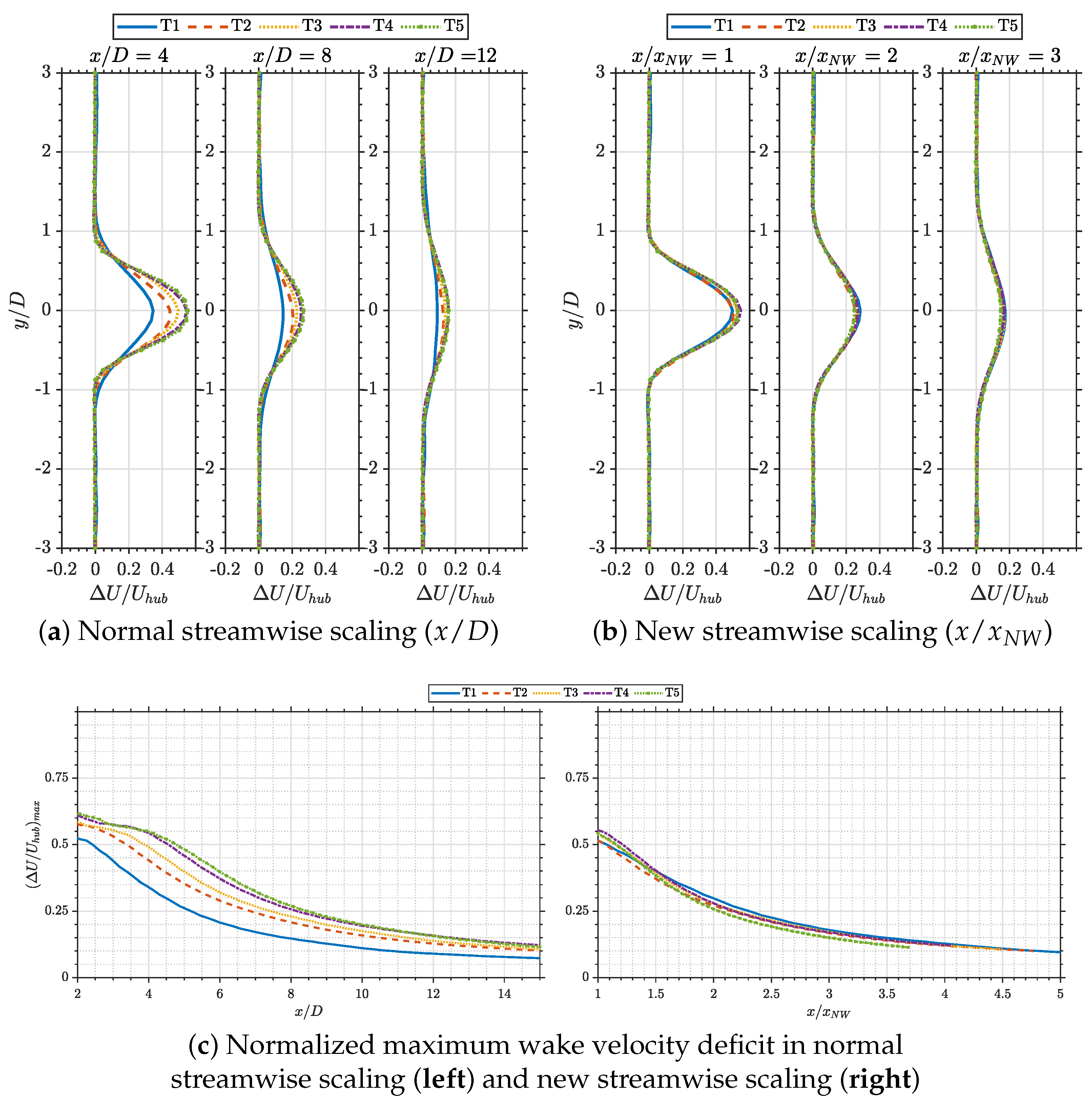
Figure 4 compares the change of the normalized wake velocity deficit for the test cases as a function of the downwind distance for the standard streamwise scaling () and the new streamwise scaling (). The figure shows a comparison between both scalings for the wake velocity deficit profiles at the turbine hub height in the plane (Figure 4a,b) and the normalized maximum velocity deficit (Figure 4c). The overlapping of the wake velocity deficit profiles and the normalized maximum velocity deficit at several downstream locations in the new streamwise coordinate demonstrates that is a relevant length scale to obtain a collapse of wake velocity deficit profiles. This new scaling introduces a self-similar behavior for the wake velocity deficit profiles under different incoming turbulent levels. The remainder of this paper explains how the new streamwise scaling can be implemented in the existing analytical wake models for wake expansion, as well as the possible computational advantages it can provide.
3.2. Application of the New Streamwise Scaling
The purpose of this section is to present two possible modeling approaches that can benefit from the new streamwise scaling. The first approach utilizes the obtained relationship derived from fitting the collapsed data of the normalized maximum wake velocity deficit to define the wake advection velocity in an explicit manner. Therefore, it is beneficial for analytical wake models with an iterative process for estimating the wake advection velocity, leading to an iterative-free streamwise-marching framework for modeling the wake mean characteristics until the desired downwind distance. Furthermore, the explicit estimation of the wake advection velocity enables calculation of the wake velocity deficit at a particular downwind location without marching and solving the wake flow for the whole upstream domain. The second approach uses the obtained relationship for the collapsed data of the normalized maximum wake velocity deficit in the new streamwise coordinate () as a stand-alone model to predict the wake velocity deficit as a function of downwind distance in the far wake. In the rest of this paper, we discuss the above-mentioned approaches in more detail and assess their performance by comparing their predictions against LES data of a real-scale wind turbine wake, presented in Table 1 as validation cases.
For practical reasons and ease of implementation in the existing analytical wake models for wake expansion, we derive a functional form for the collapsed data of the normalized maximum wake velocity deficit as a function of the new streamwise scaling. The collapsed curve is normalized by the maximum wake velocity deficit derived from one-dimensional momentum theory () [36]. In this regard, we propose the following form for the normalized maximum wake velocity deficit in the new streamwise coordinate ():
in which is the turbine thrust coefficient and the values of a, b, and c should be estimated. This form is valid in the far wake (), and ensures that the wake velocity deficit is equal to the theoretical limit at the beginning of the far wake and asymptotes to zero in the very far wake. Figure 5 shows the change in the collapsed data of the normalized maximum wake velocity deficit for the test cases as a function of the new streamwise distance, as well as the fitted curve. The data used for fitting correspond to the far wake region of each test case, from the end of the near-wake to 30 rotor diameters downwind. The parameters of the fitted function are reported in Table 2.
3.2.1. Coupled with the Existing Analytical Models for Wake Expansion
This section focuses on how the new streamwise scaling can be incorporated as part of the existing analytical model for wake expansion proposed by Vahidi and Porté-Agel [10]. This physics-based model for wake expansion is based on the application of Taylor diffusion theory [9], turbulent mixing layers [14], the Gaussian wake model [4], and the analogy between scalar diffusion from a disk source and wind turbine wake expansion [37]. The model includes the turbine-induced turbulence and the ambient turbulence effects on the wake expansion. As a result, the model conserves mass and momentum in the far wake and provides reasonable predictions of the wake width and maximum velocity deficit within a wide range of incoming turbulence levels. To estimate the wake width at each downstream distance, the model solves the spreading equation for the lateral mixing layer characteristic length () growing from the end of the expansion region ():
where is the turbulent Schmidt number for mixing layers [38] and is the mixing layer spreading rate. Here, is the root mean square of the lateral velocity component sampled upstream of the turbine at hub level and filtered in time using a moving average filter with the window size equal to , with the Lagrangian/Eulerian scale factor () [39] and T the travel time:
where is the wake advection velocity. The wake advection velocity is defined as , with the wake centerline velocity [40]. It should be mentioned here that there is no limitation to extend Equation (4) to the vertical direction with the respective velocity time series. The total wake width is defined as the geometrical mean of wake widths in the vertical and spanwise directions () [8,16]. To conserve mass and momentum in the far wake, the wake centerline velocity is calculated using the Gaussian wake model. In the near-wake, the wake centerline velocity is assumed to be constant and equal to the value derived from the one-dimensional momentum theory (). In order to calculate the Gaussian wake width in the far wake from the corresponding mixing layer characteristic length, the proposed analogy between scalar diffusion from the disk source and wind turbine wake expansion is employed. This analogy results in a unique relationship between the wind turbine wake width () and the mixing layer characteristic length ():
Equation (4), hereafter referred to as the Model Filter, requires an external function to filter the velocity time series at each downstream distance. In order to remove the dependency on the external function and provide a compact version of the model, the following equation (hereafter referred to as Model ITS, in which ITS stands for Integral Time Scale) was derived based on the exponential form of the velocity auto-correlation function [9,41]. This equation estimates the wake width at each downwind distance based on the travel time, unfiltered velocity standard deviation, and the integral scale of the incoming atmospheric flow [10]:
where is the Lagrangian integral time scale for the lateral velocity time series and is the lateral velocity component standard deviation. Equation (7) has the same range of validity as the Model Filter, from the end of the expansion region (≈) until the desired downwind distance. As with Equation (4), Equation (7) can be used to calculate the vertical wake width with the respective properties.
Within the framework of this model, Vahidi and Porté-Agel [10] proposed a near-wake length relation to calculate the starting point of the far wake based on the incoming flow turbulence levels and turbine operating condition, as follows:
where determines the beginning of the far wake based on the Gaussian fit correlation coefficient () of 0.99 and the analogy used in the model. This relationship includes the contribution of the relevant incoming turbulence scales to wake expansion until the end of the near-wake by utilizing the equivalent filtered velocity of the incoming flow. Equation (8) requires an iterative method to solve for the length of the near-wake. In order to provide a simpler form for calculating this length, Vahidi and Porté-Agel [10] proposed the following simplification for Equation (8):
In both the Model Filter and Model ITS, the wake centerline velocity at each downwind distance is unknown prior to finding the mixing layer characteristic length and wake width. Therefore, one should deploy an iterative scheme to estimate the wake centerline velocity and the corresponding travel time, following the steps described in the original model. As an outcome of the new streamwise scaling, the wake advection velocity can be calculated by re-scaling the collapsed profile of the normalized maximum wake velocity deficit (Equation (3)) with an estimation of the near-wake length and calculating the wake centerline velocity from the maximum wake velocity deficit (). With the wake advection velocity, it is possible to estimate the travel time in the entire domain of interest before running the model by calculating the integral of Equation (5) numerically. As a result, it is no longer necessary to iterate between the mixing layer characteristic length and the travel time at each downwind distance, which leads to considerable speedup of the calculation process.
Another important outcome of the new streamwise scaling in the context of analytical models for wake expansion is to remove the need for streamwise marching to estimate the wake mean properties at a certain downwind distance. In the iterative version of the Model Filter and Model ITS, the domain must be discretized up to the point of interest in order to estimate the wake velocity deficit at a given downwind distance, and the analytical model for each upstream point must be solved prior to calculating the wake velocity deficit at the location of interest. In contrast, the new streamwise scaling allows the wake velocity deficit to be estimated at a desired downwind distance using the Model Filter or Model ITS, without the need to discretize the entire domain up to the point of interest. A direct estimation of the travel time at the desired location can be obtained by re-scaling the collapsed profile of the normalized maximum wake velocity deficit and estimating the wake advection velocity. The travel time can be inserted directly in the Model Filter (Equation (4)) or Model ITS (Equation (7)) to estimate the mixing layer characteristic length and the corresponding wake width and wake velocity deficit.
In order to test the performance of the Model Filter and Model ITS in predicting the wake velocity deficit downwind of a turbine with the new streamwise scaling, we compare their outputs against the LES data presented in Table 1 as validation cases. To run the models, the step-by-step procedure provided in the original derivation is followed, together with the same set of parameters (, , , ) [10]. For the sake of comparison, both models are used in their original form (iterative form denoted as original) and with the new streamwise scaling (non-iterative form denoted as new scaling).
The change in the maximum normalized velocity deficit at the turbine hub height downwind of the turbine derived from the analytical models is shown in Figure 6, and is compared with value derived from the LES data. In this comparison, we evaluate how accurately wake expansion models coupled with the new scaling can predict the wake maximum velocity deficits as they march the streamwise distance until 15 rotor diameters. As can be observed, both models (in both iterative and non-iterative form) can predict the variation of the normalized wake velocity deficit reasonably well. The models can predict the wake velocity deficit at distances close to the turbine and provide the correct asymptotic behavior in the far wake. This figure provides an interesting comparison between iterative and non-iterative approaches to solve each model. By introducing the new streamwise scaling, the Model Filter and Model ITS predict the development of the wake velocity deficit with the same level of accuracy as the original (iterative) form, and with less computational cost. For the results reported in Figure 6, by virtue of the new streamwise scaling, the computational cost of the non-iterative form of the Model Filter and Model ITS decreases by 35% and 45%, respectively, in comparison with their iterative counterparts. This computational efficiency is a significant factor for fast-running wake engineering models. Later in this section, a detailed analysis of the computational efficiency of the analytical models coupled with the new scaling for predicting the wake velocity deficit at one specific downwind location is presented.
3.2.2. Stand-Alone Model
The functional form obtained from the collapse of the normalized maximum wake velocity deficit as a function of () (Equation (3)) can be used as a computationally fast approach to calculate the maximum wake velocity deficit as a function of the downstream distance in the far wake with an estimation of the near-wake length as an input. In order to conserve mass and momentum in the far wake, the Gaussian wake model can be used to calculate the wake width and determine the wake velocity deficit distribution. Considering that the proposed method uses only a few arithmetical operations, its computational cost is insignificant in comparison with streamwise-marching techniques.
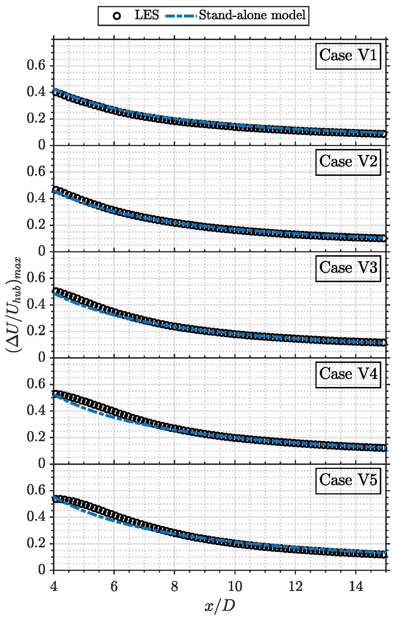
Following the comparisons presented in Section 3.2.1, our purpose is to test how accurately the re-scaling of the functional form obtained for the normalized maximum wake velocity deficit collapsed data (hereafter referred to as the stand-alone model) can predict the change in the wake velocity in the far wake by comparing its predictions against the LES data of the validation cases. To use the stand-alone model, an estimation of the near-wake length is required. Equation (8) is used to estimate the near-wake length using the same set of parameters as the original derivation (, , , ) [10]. Figure 7 shows the change in the maximum wake velocity deficit computed with the stand-alone model and that obtained from LES data. As can be seen, the stand-alone model provides the correct asymptotic behavior for the wake velocity deficit in the far wake at downstream distances greater than 10 rotor diameters. For shorter distances from the turbine (up to downwind distances of about 5 to 7 rotor diameters) and for cases with lower incoming turbulence levels, the stand-alone model underestimates the wake velocity deficit compared to the LES data. The same trend can be observed when the predictions are compared with the physics-based models presented in Figure 6. This difference can be explained by the underlying modeling approach used by each analytical wake model to estimate the maximum wake velocity deficit at a certain downwind distance. Within the framework of the physics-based wake expansion model, the wake width at each streamwise position is estimated by explicitly using the turbine-induced turbulence and the effective incoming turbulence scales. On the other hand, the stand-alone model accounts for these effects indirectly through their impact on the near-wake length, rendering the model more sensitive to the accuracy of the estimated near-wake length and the goodness of the fit to the collapsed data of the normalized wake velocity deficit.
3.2.3. Effect of the Near-Wake Length Relation
The application of the new streamwise scaling, either integrated into the existing analytical models for wake expansion (Section 3.2.1) or used as the stand-alone model (Section 3.2.2), relies on estimation of the near-wake length. The near-wake length is a function of the incoming turbulence characteristics and turbine operating conditions. In this section, we examine the sensitivity of the discussed approaches to the relation used to calculate the near-wake length. In order to do this, different relations for estimating the near-wake length are used to re-scale the collapsed profile of the normalized maximum wake velocity deficit. Next, the re-scaled normalized maximum wake velocity deficit is used as either part of the existing analytical model for the wake expansion (to calculate the wake advection velocity) or as the stand-alone model.
This analysis includes three different relations used to estimate the near-wake length. First, the near-wake relation proposed by Vahidi and Porté-Agel [10] (referred to in the figure as VPA) as stated in Equation (8); second, the near-wake length relation proposed by Bastankhah and Porté-Agel [17] as the potential core model (referred to in the figure as BPA):
with and ; and third, the near-wake length model presented by Vermeulen [42] (referred to in the figure as Verm):
where , , and is defined as
where , , and , with B being the number of blades and the tip speed ratio. Figure 8 shows the variation of the near-wake length of the validation cases as a function of the streamwise turbulence intensity, computed from the presented relations as well as from that obtained from LES data, following the method introduced in Section 3. As can be observed, decreasing the turbulence level means that the wake requires a longer distance to reach a self-similar Gaussian state. This behavior is captured reasonably well by the relations for the near wake proposed by Bastankhah and Porté-Agel [17] and by Vahidi and Porté-Agel [10].
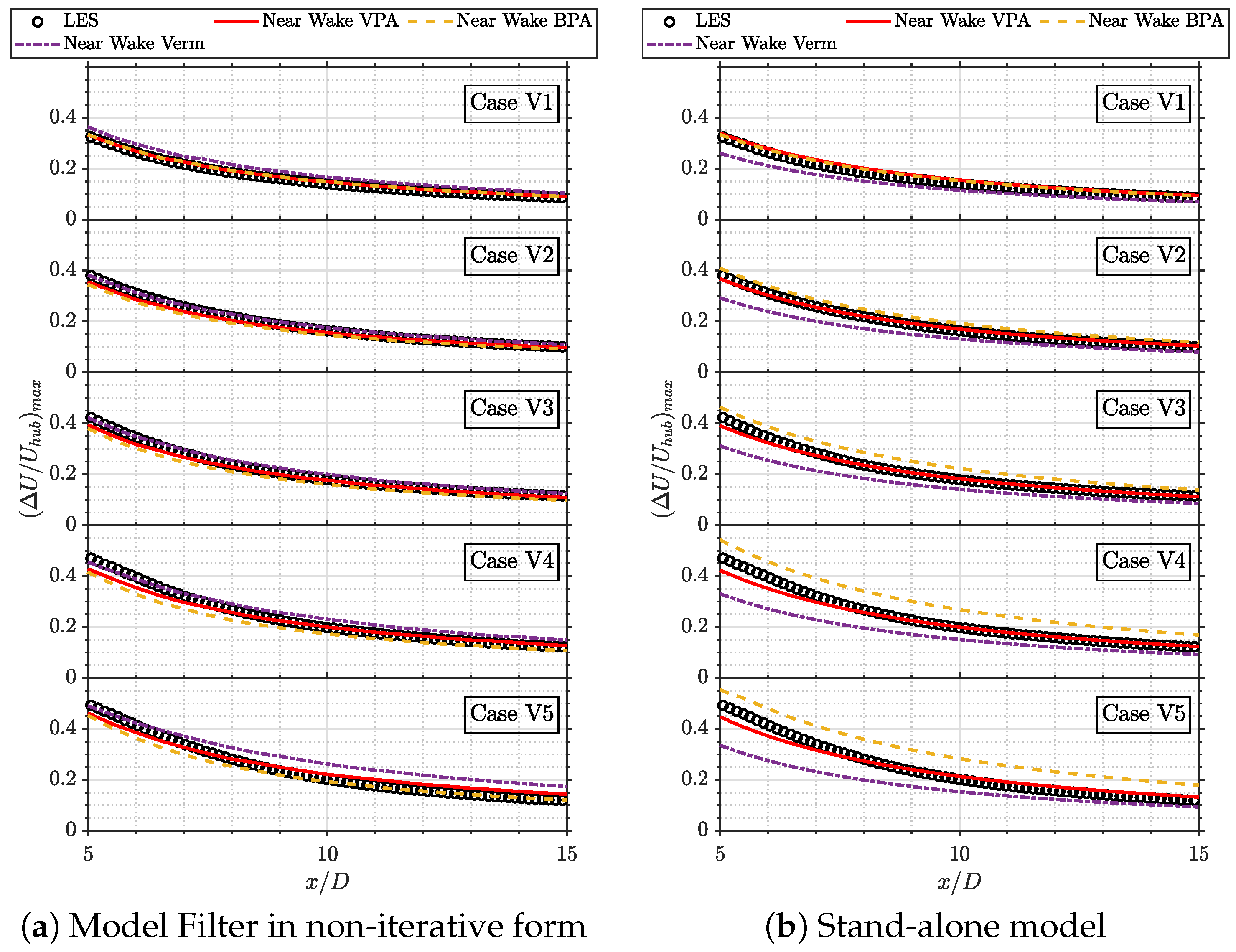
Figure 9a shows the change in the maximum wake velocity deficit at turbine hub height as a function of the downwind distance computed from the Model Filter (in non-iterative form) and that obtained from the validation case LES data. In order to use the Model Filter, the travel time is calculated by re-scaling the relationship obtained from fitting the collapsed data of the normalized maximum wake velocity deficit with different near-wake relations. For the sake of brevity and based on the identical performance of the Model Filter and Model ITS (Section 3.2.1), only the results for the Model Filter are reported in the figure. Figure 9b shows the comparison between the change in the maximum velocity deficit as a function of the downwind distance computed from the stand-alone model and the validation case LES data. The only parameter required for the stand-alone model is the near-wake length, which is calculated based on the previously stated relations.
As shown in Figure 9, the predictions of the Model Filter are less sensitive to the near-wake length relation at downwind distances up to 6 to 10 rotor diameters as compared to the stand-alone model. This can be explained by the fact that physics-based analytical models for the wake expansion include the contribution of the effective turbulence scales and the turbine-induced turbulence to the wake width at each downwind distance. As a result, their predictions are fairly robust against variability in the near-wake length estimate. As can be noticed from Figure 9a, all of the approaches provide consistent behavior in the far wake at downstream distances greater than 12 rotor diameters. It is worth mentioning that the near-wake relations proposed by Vahidi and Porté-Agel [10] and Bastankhah and Porté-Agel [17] show similar behavior when used in the context of physics-based analytical models for wake expansion. This is due to the rather similar concepts underlying the derivation of these relations and a more realistic description for the wake development until the end of the near-wake, profiting from plausible analogies with jet flows [17] and from the analogy between scalar diffusion from a disk source and wind turbine wake expansion [10]. As shown in Figure 9b, the performance of the stand-alone model is highly dependent on the relation used to calculate the length of the near-wake, as this is the only required input. The stand-alone model coupled with the near-wake relation proposed by Vahidi and Porté-Agel [10] provides a reasonable prediction of the wake velocity deficit compared with the LES data. On the other hand, the stand-alone model coupled with the Vermeulen [42] and Bastankhah and Porté-Agel [17] relations underestimates or overestimates the change in the wake velocity deficit with the downwind distance.
3.2.4. Computational Efficiency
After evaluating the performance of the above-mentioned analytical models for wake expansion against the LES data, this section focuses on the computational advantages of the new streamwise scaling for the presented analytical models. In order to do this, the computational time taken by each model to estimate the wake velocity deficit at a specific downwind location is determined. To make comparisons, we use a downwind location at 8 rotor diameters. This distance is of particular relevance, as it falls within the typical range of turbine spacings found in wind farms [1]. In order to estimate the wake velocity deficit at 8 rotor diameters for all the validation cases, the iterative form of the Model Filter and Model ITS requires discretization of the downwind distance and streamwise marching to solve the wake flow from the end of the expansion region to the point of interest. However, their non-iterative counterparts take advantage of the new streamwise scaling to calculate the wake advection velocity and the corresponding travel time at the location of interest, which means they only need to solve the necessary equations once. Similarly, the stand-alone model only requires the near-wake length estimation in order to calculate the wake velocity deficit at 8 rotor diameters.
Figure 10 compares the mean relative computational cost of the Model Filter and Model ITS (in both iterative and non-iterative form) with the stand-alone model for all the validation cases. Equation (8) is used to calculate the near-wake length in all the reported results. Because the iterative form of the Model Filter is the least computationally efficient model, the reported values are normalized with its computational time. As can be noticed in the figure, by introducing the streamwise scaling and eliminating the need to discretize the whole domain up to the point of interest both the Model Filter and Model ITS are one order of magnitude faster compared to their respective original iterative implementations. Among all the presented approaches, the stand-alone model proves to be the fastest. It is worth mentioning that the comparison between the Model Filter and Model ITS in iterative form reveals the computational advantages of removing the need to explicitly filter the velocity time-series using an external moving average function.
4. Summary and Concluding Remarks
In this paper, a new streamwise scaling for wind turbine wakes under neutral atmospheric conditions has been presented, and the practical applications of the proposed scaling for analytical wake models have been discussed. For this purpose, large-eddy simulations of a real-scale wind turbine under neutral atmospheric conditions, with a wide range of incoming turbulence levels, have been performed. The simulations have been divided into two sets: test cases and validation cases. Test cases have been used to evaluate the validity of the proposed research question regarding the new streamwise coordinate system, and validation cases to assess the performance of analytical wake models.
Aiming to find a common behavior of the wake velocity deficit under a wide range of inflow conditions, the near-wake length, as a measure of the wake self-similar region onset, has been chosen as a proper length scale. By normalizing the streamwise distance with the near-wake length, a collapse of the normalized far wake velocity deficit profiles under different incoming turbulence levels has been observed. A functional form has been obtained by fitting the collapsed data of the normalized maximum wake velocity deficit in the far wake.
Two approaches for predicting the wake velocity deficit based on the new streamwise scaling have been proposed. First, by profiting from the relationship obtained by fitting the collapsed data of the normalized maximum wake velocity deficit, the wake advection velocity has been estimated explicitly. By coupling this explicit form with the existing physics-based wake expansion model, a non-iterative version of this model has been presented, which led to a considerable speed-up in the calculation. Second, a stand-alone model has been proposed and only requires as input the near-wake length to predict the wake velocity deficit as a function of the downstream distance in the far wake. The performance of both approaches has been evaluated against LES results of a utility-scale wind turbine wake under a wide range of incoming turbulence levels. In a comparison focused on predicting the wake velocity deficit until 15 rotor diameters, the physics-based wake expansion model (in both original and simplified versions) yields reasonable predictions of the wake velocity deficit for all the LES cases. Moreover, the mean computational cost of the non-iterative versions of the physics-based wake expansion model decreases considerably in comparison with the iterative counterparts (around 35% for the original version and 45% for the simplified version). The stand-alone model underestimates the wake velocity deficit close to the turbine while providing a correct asymptotic behavior in downwind distances greater than 10 rotor diameters. The sensitivity of the proposed approaches to the relation used to calculate the near-wake length has been examined. While the stand-alone model predictions showed to be sensitive to the relation used to estimate the near-wake length, the results of the physics-based model for the wake expansion proved to be robust to variability in the estimation of the near-wake length. In particular, it is noteworthy to mention that in the case of predicting the wake velocity deficit at a certain downwind distance, the physics-based wake expansion model, by taking advantage of the new scaling and removing the need for streamwise-marching until the desired downwind distance, can predict the wake velocity deficit at a particular downwind location one order of magnitude faster than their original implementation (with streamwise-marching) with the same level of accuracy.
In summary, the detailed comparison between the analytical models for the wake expansion and LES data demonstrates that the new streamwise scaling, in combination with the physics-based wake models, can provide an accurate and fast prediction of wind turbine wake flows under a wide range of incoming turbulence levels.
Author Contributions
Conceptualization, D.V. and F.P.-A.; data curation, D.V.; formal analysis, D.V.; funding acquisition, F.P.-A.; investigation, D.V. and F.P.-A.; methodology, D.V. and F.P.-A.; project administration, F.P.-A.; resources, F.P.-A.; software, D.V.; supervision, F.P.-A.; validation, D.V.; visualization, D.V.; writing—original draft, D.V.; writing—review and editing, D.V. and F.P.-A. All authors have read and agreed to the published version of the manuscript.
Funding
This research was funded by the Swiss Federal Office of Energy (Grant Number SI/502135-01).
Data Availability Statement
The data presented in this study are available from the corresponding author on request.
Acknowledgments
Computing resources were provided by EPFL through the use of the facilities of its Scientific IT and Application Support Center (SCITAS) and by the Swiss National Supercomputing Centre (CSCS).
Conflicts of Interest
The authors declare no conflict of interest.
References
- Porté-Agel, F.; Bastankhah, M.; Shamsoddin, S. Wind-turbine and wind-farm flows: A review. Bound.-Layer Meteorol. 2020, 174, 1–59. [Google Scholar] [CrossRef] [PubMed] [Green Version]
- Jensen, N. A Note on Wind Turbine Interaction; Riso-M-2411; Risoe National Laboratory: Roskilde, Denmark, 1983; p. 16. [Google Scholar]
- Frandsen, S.; Barthelmie, R.; Pryor, S.; Rathmann, O.; Larsen, S.; Højstrup, J.; Thøgersen, M. Analytical modelling of wind speed deficit in large offshore wind farms. Wind Energy Int. J. Prog. Appl. Wind Power Convers. Technol. 2006, 9, 39–53. [Google Scholar] [CrossRef]
- Bastankhah, M.; Porté-Agel, F. A new analytical model for wind-turbine wakes. Renew. Energy 2014, 70, 116–123. [Google Scholar] [CrossRef]
- Brugger, P.; Fuertes, F.C.; Vahidzadeh, M.; Markfort, C.D.; Porté-Agel, F. Characterization of Wind Turbine Wakes with Nacelle-Mounted Doppler LiDARs and Model Validation in the Presence of Wind Veer. Remote Sens. 2019, 11, 2247. [Google Scholar] [CrossRef] [Green Version]
- Teng, J.; Markfort, C.D. A Calibration Procedure for an Analytical Wake Model Using Wind Farm Operational Data. Energies 2020, 13, 3537. [Google Scholar] [CrossRef]
- Niayifar, A.; Porté-Agel, F. Analytical modeling of wind farms: A new approach for power prediction. Energies 2016, 9, 741. [Google Scholar] [CrossRef] [Green Version]
- Cheng, W.C.; Porté-Agel, F. A simple physically-based model for wind-turbine wake growth in a turbulent boundary layer. Bound.-Layer Meteorol. 2018, 169, 1–10. [Google Scholar] [CrossRef]
- Taylor, G.I. Diffusion by continuous movements. Proc. Lond. Math. Soc. 1922, 2, 196–212. [Google Scholar] [CrossRef]
- Vahidi, D.; Porté-Agel, F. A physics-based model for wind turbine wake expansion in the atmospheric boundary layer. J. Fluid Mech. 2022, 943, A49. [Google Scholar] [CrossRef]
- Townsend, A. The Structure of Turbulent Shear Flow; Cambridge University Press: Cambridge, UK, 1980. [Google Scholar]
- Tennekes, H.; Lumley, J.L.; Lumley, J.L. A First Course in Turbulence; MIT Press: Cambridge, MA, USA, 1972. [Google Scholar]
- George, W.K. The self-preservation of turbulent flows and its relation to initial conditions and coherent structures. Adv. Turbul. 1989, 3973. [Google Scholar]
- Pope, S.B. Turbulent Flows; Cambridge University Press: Cambridge, UK, 2001. [Google Scholar]
- Xie, S.; Archer, C. Self-similarity and turbulence characteristics of wind turbine wakes via large-eddy simulation. Wind Energy 2015, 18, 1815–1838. [Google Scholar] [CrossRef]
- Abkar, M.; Porté-Agel, F. Influence of atmospheric stability on wind-turbine wakes: A large-eddy simulation study. Phys. Fluids 2015, 27, 035104. [Google Scholar] [CrossRef] [Green Version]
- Bastankhah, M.; Porté-Agel, F. Experimental and theoretical study of wind turbine wakes in yawed conditions. J. Fluid Mech. 2016, 806, 506–541. [Google Scholar] [CrossRef]
- Dar, A.S.; Porté-Agel, F. Wind turbine wakes on escarpments: A wind-tunnel study. Renew. Energy 2022, 181, 1258–1275. [Google Scholar] [CrossRef]
- Shamsoddin, S.; Porté-Agel, F. A model for the effect of pressure gradient on turbulent axisymmetric wakes. J. Fluid Mech. 2018, 837, R3. [Google Scholar] [CrossRef]
- Dar, A.S.; Porté-Agel, F. An Analytical Model for Wind Turbine Wakes under Pressure Gradient. Energies 2022, 15, 5345. [Google Scholar] [CrossRef]
- Shamsoddin, S.; Porté-Agel, F. Effect of aspect ratio on vertical-axis wind turbine wakes. J. Fluid Mech. 2020, 889, R1. [Google Scholar] [CrossRef]
- Meunier, P.; Spedding, G.R. A loss of memory in stratified momentum wakes. Phys. Fluids 2004, 16, 298–305. [Google Scholar] [CrossRef]
- Li, Z.; Yang, X. Large-eddy simulation on the similarity between wakes of wind turbines with different yaw angles. J. Fluid Mech. 2021, 921, A11. [Google Scholar] [CrossRef]
- Uddin, M.; Pollard, A. Self-similarity of coflowing jets: The virtual origin. Phys. Fluids 2007, 19, 068103. [Google Scholar] [CrossRef]
- Stoll, R.; Porté-Agel, F. Dynamic subgrid-scale models for momentum and scalar fluxes in large-eddy simulations of neutrally stratified atmospheric boundary layers over heterogeneous terrain. Water Resour. Res. 2006, 42, W01409. [Google Scholar] [CrossRef]
- Wu, Y.T.; Porté-Agel, F. Large-eddy simulation of wind-turbine wakes: Evaluation of turbine parametrisations. Bound.-Layer Meteorol. 2011, 138, 345–366. [Google Scholar] [CrossRef]
- Porté-Agel, F.; Wu, Y.T.; Lu, H.; Conzemius, R.J. Large-eddy simulation of atmospheric boundary layer flow through wind turbines and wind farms. J. Wind Eng. Ind. Aerodyn. 2011, 99, 154–168. [Google Scholar] [CrossRef]
- Wu, Y.T.; Porté-Agel, F. Modeling turbine wakes and power losses within a wind farm using LES: An application to the Horns Rev offshore wind farm. Renew. Energy 2015, 75, 945–955. [Google Scholar] [CrossRef]
- Wu, Y.T.; Porté-Agel, F. Atmospheric turbulence effects on wind-turbine wakes: An LES study. Energies 2012, 5, 5340–5362. [Google Scholar] [CrossRef] [Green Version]
- Revaz, T.; Porté-Agel, F. Large-Eddy Simulation of Wind Turbine Flows: A New Evaluation of Actuator Disk Models. Energies 2021, 14, 3745. [Google Scholar] [CrossRef]
- Lin, M.; Porté-Agel, F. Large-eddy Simulation of a Wind-turbine Array subjected to Active Yaw Control. Wind Energ. Sci. 2022, 7, 2215–2230. [Google Scholar] [CrossRef]
- Mikkelsen, R. Actuator Disc Methods Applied to Wind Turbines. Ph.D. Thesis, Technical University of Denmark, Lyngby, Denmark, 2003. [Google Scholar]
- Chamorro, L.P.; Porté-Agel, F. A wind-tunnel investigation of wind-turbine wakes: Boundary-layer turbulence effects. Bound.-Layer Meteorol. 2009, 132, 129–149. [Google Scholar] [CrossRef] [Green Version]
- Carbajo Fuertes, F.; Markfort, C.D.; Porté-Agel, F. Wind turbine wake characterization with nacelle-mounted wind lidars for analytical wake model validation. Remote Sens. 2018, 10, 668. [Google Scholar] [CrossRef] [Green Version]
- Sørensen, J.N.; Mikkelsen, R.F.; Henningson, D.S.; Ivanell, S.; Sarmast, S.; Andersen, S.J. Simulation of wind turbine wakes using the actuator line technique. Philos. Trans. R. Soc. A Math. Phys. Eng. Sci. 2015, 373, 20140071. [Google Scholar] [CrossRef] [Green Version]
- Hansen, M.O. Aerodynamics of Wind Turbines; Routledge: London, UK, 2015. [Google Scholar]
- Crank, J. The Mathematics of Diffusion; Oxford University Press: New York, NY, USA, 1979. [Google Scholar]
- Reynolds, A. The variation of turbulent Prandtl and Schmidt numbers in wakes and jets. Int. J. Heat Mass Transf. 1976, 19, 757–764. [Google Scholar] [CrossRef]
- Hanna, S. Lagrangian and Eulerian time-scale relations in the daytime boundary layer. J. Appl. Meteorol. 1981, 20, 242–249. [Google Scholar] [CrossRef]
- Zong, H.; Porté-Agel, F. A momentum-conserving wake superposition method for wind farm power prediction. J. Fluid Mech. 2020, 889, A8. [Google Scholar] [CrossRef]
- Neumann, J. Some observations on the simple exponential function as a Lagrangian velocity correlation function in turbulent diffusion. Atmos. Environ. 1978, 12, 1965–1968. [Google Scholar] [CrossRef]
- Vermeulen, P. An experimental analysis of wind turbine wakes. In Proceedings of the 3rd International Symposium on Wind Energy Systems, Lyngby, Denmark, 26–29 August 1980; pp. 431–450. [Google Scholar]
Figure 1.
Inflow characteristic for test cases: (a) vertical profiles of the mean streamwise velocity normalized with the friction velocity () compared to the log law (dashed line); (b) vertical profiles of the normalized mean streamwise velocity in linear scale; (c) vertical profiles of the mean streamwise turbulence intensity.

Figure 2.
Contours of the normalized mean streamwise velocity () in the plane, passing through the center of the turbine for (a) T1, (b) T5, (c) V1, (d) V5.
Figure 2.
Contours of the normalized mean streamwise velocity () in the plane, passing through the center of the turbine for (a) T1, (b) T5, (c) V1, (d) V5.

Figure 3.
An example of the near-wake length calculation method for Case T5. The same analysis was performed for all the cases in Table 1 to determine the near-wake length, and is not reported here for brevity.
Figure 3.
An example of the near-wake length calculation method for Case T5. The same analysis was performed for all the cases in Table 1 to determine the near-wake length, and is not reported here for brevity.

Figure 4.
Evaluating the research question: comparison of the lateral wake velocity deficit profiles in (a) normal streamwise scaling and (b) new streamwise scaling; (c) comparison of the normalized maximum wake velocity deficit behaviour under two different streamwise scalings.
Figure 4.
Evaluating the research question: comparison of the lateral wake velocity deficit profiles in (a) normal streamwise scaling and (b) new streamwise scaling; (c) comparison of the normalized maximum wake velocity deficit behaviour under two different streamwise scalings.

Figure 5.
Collapsed profile of the normalized maximum wake velocity deficit for the test cases as a function of the new streamwise scaling. The dashed line corresponds to the fitted function.
Figure 5.
Collapsed profile of the normalized maximum wake velocity deficit for the test cases as a function of the new streamwise scaling. The dashed line corresponds to the fitted function.

Figure 6.
Normalized maximum velocity deficit as a function of streamwise distance. The circles indicate LES results, the lines show the models in their original (iterative) form, and the symbols indicate the model outputs with the new scaling (non-iterative): (a) Model Filter and (b) Model ITS.
Figure 6.
Normalized maximum velocity deficit as a function of streamwise distance. The circles indicate LES results, the lines show the models in their original (iterative) form, and the symbols indicate the model outputs with the new scaling (non-iterative): (a) Model Filter and (b) Model ITS.

Figure 7.
Normalized maximum velocity deficit as a function of streamwise distance. The circles indicate LES results and the dash-dotted line corresponds to the stand-alone model.
Figure 7.
Normalized maximum velocity deficit as a function of streamwise distance. The circles indicate LES results and the dash-dotted line corresponds to the stand-alone model.

Figure 8.
Near-wake length of validation cases as a function of streamwise turbulence intensity: comparison of the presented relationships and the LES data. The symbols represent the validation cases. Equation (10) (BPA model, dashed line) and Equation (11) (Verm model, dotted line) are shown for comparison. Figure adapted from Vahidi and Porté-Agel [10].

Figure 9.
Normalized maximum velocity deficit as a function of streamwise distance: a comparison of the effect of different near-wake relations on the analytical model outputs. (a) Model Filter in non-iterative form with different near-wake length relations; (b) stand-alone model with different near-wake length relations.

Figure 10.
Relative computational time of the presented analytical models to estimate the wake velocity deficit at a downwind distance of 8 rotor diameters.
Figure 10.
Relative computational time of the presented analytical models to estimate the wake velocity deficit at a downwind distance of 8 rotor diameters.


Table 1.
Suite of LES simulations. Test cases and validation cases are denoted by T and V, respectively, while respectively correspond to the streamwise, spanwise, and vertical rotor-averaged turbulence intensity. The test cases are adapted from Vahidi and Porté-Agel [10].
Table 1.
Suite of LES simulations. Test cases and validation cases are denoted by T and V, respectively, while respectively correspond to the streamwise, spanwise, and vertical rotor-averaged turbulence intensity. The test cases are adapted from Vahidi and Porté-Agel [10].
| Case | Roughness (m) | |||||
|---|---|---|---|---|---|---|
| T1 | 0.140 | 0.097 | 0.074 | |||
| T2 | 0.099 | 0.071 | 0.055 | |||
| T3 | 0.077 | 0.055 | 0.043 | |||
| T4 | 0.062 | 0.044 | 0.034 | |||
| T5 | 0.053 | 0.038 | 0.029 | |||
| V1 | 0.127 | 0.076 | 0.056 | |||
| V2 | 0.080 | 0.058 | 0.046 | |||
| V3 | 0.066 | 0.047 | 0.037 | |||
| V4 | 0.056 | 0.038 | 0.031 | |||
| V5 | 0.049 | 0.034 | 0.027 |
Table 2.
Fitting parameters of Equation (3); corresponds to the fit correlation coefficient.
Table 2.
Fitting parameters of Equation (3); corresponds to the fit correlation coefficient.
| a | b | c | |
|---|---|---|---|
| 1.75 | −0.5 | −1.37 | 0.99 |
Publisher’s Note: MDPI stays neutral with regard to jurisdictional claims in published maps and institutional affiliations. |
© 2022 by the authors. Licensee MDPI, Basel, Switzerland. This article is an open access article distributed under the terms and conditions of the Creative Commons Attribution (CC BY) license (https://creativecommons.org/licenses/by/4.0/).
Share and Cite
MDPI and ACS Style
Vahidi, D.; Porté-Agel, F. A New Streamwise Scaling for Wind Turbine Wake Modeling in the Atmospheric Boundary Layer. Energies 2022, 15, 9477. https://0-doi-org.brum.beds.ac.uk/10.3390/en15249477
AMA Style
Vahidi D, Porté-Agel F. A New Streamwise Scaling for Wind Turbine Wake Modeling in the Atmospheric Boundary Layer. Energies. 2022; 15(24):9477. https://0-doi-org.brum.beds.ac.uk/10.3390/en15249477
Chicago/Turabian StyleVahidi, Dara, and Fernando Porté-Agel. 2022. "A New Streamwise Scaling for Wind Turbine Wake Modeling in the Atmospheric Boundary Layer" Energies 15, no. 24: 9477. https://0-doi-org.brum.beds.ac.uk/10.3390/en15249477
Note that from the first issue of 2016, this journal uses article numbers instead of page numbers. See further details here.