

Multivariate Data-Driven Models for Wind Turbine Power Curves including Sub-Component Temperatures

1
Department of Engineering, University of Perugia, Via G. Duranti 93, 06125 Perugia, Italy
2
Centre for Life-Cycle Engineering and Management (CLEM), School of Aerospace Transport and Manufacturing, Cranfield University, Bedford MK43 0AL, UK
3
ENGIE Italia, Via Chiese, 20126 Milano, Italy
*
Author to whom correspondence should be addressed.
Energies 2023, 16(1), 165; https://0-doi-org.brum.beds.ac.uk/10.3390/en16010165
Submission received: 15 November 2022
/
Revised: 13 December 2022
/
Accepted: 19 December 2022
/
Published: 23 December 2022
(This article belongs to the Special Issue Decision-Making Systems in Power System Planning and Operation in the Presence of High Shares of Renewable Energies)
Abstract
:The most commonly employed tool for wind turbine performance analysis is the power curve, which is the relation between wind intensity and power. The diffusion of SCADA systems has boosted the adoption of data-driven approaches to power curves. In particular, a recent research line involves multivariate methods, employing further input variables in addition to the wind speed. In this work, an innovative contribution is investigated, which is the inclusion of thirteen sub-component temperatures as possible covariates. This is discussed through a real-world test case, based on data provided by ENGIE Italia. Two models are analyzed: support vector regression with Gaussian kernel and Gaussian process regression. The input variables are individuated through a sequential feature selection algorithm. The sub-component temperatures are abundantly selected as input variables, proving the validity of the idea proposed in this work. The obtained error metrics are lower with respect to benchmark models employing more typical input variables: the resulting mean absolute error is 1.35% of the rated power. The results of the two types of selected regressions are not remarkably different. This supports that the qualifying points are, rather than the model type, the use and the selection of a potentially vast number of input variables.
1. Introduction
Horizontal-axis wind turbines are rotating machines which operate under non-stationary conditions because the source is stochastic. Furthermore, the power extracted by a wind turbine has a complex dependence on working parameters and environmental conditions. Based on theoretical arguments [1], the expected power production is given in Equation (1):
In Equation (1), P is the produced power and depends on the rotor radius R, the air density , the wind speed v, and the power coefficient , which depends on the blade pitch angle and the tip-speed ratio (or, in other words, the rotational speed ).
In Equation (1), v is intended to be the longitudinal wind intensity. Most of the complications regarding wind turbine performance monitoring [2] are related to the fact that what is measured using the most adopted sensory systems is not exactly v. Typically, wind turbines are equipped with cup anemometers measuring the wind flow behind the rotor span, and the undisturbed wind speed v is estimated ex post through a nacelle transfer function. This procedure has intrinsic limitations because the nacelle transfer function is calibrated only in some sample representative environmental conditions. Without the use of additional sensors on site, whose use in the industry practice is discouraged by costs and benefits considerations, the effects of vertical components of the wind flow [3], turbulence intensity [4], humidity, temperature [5], and so on are substantially discarded.
The design specifications of a wind turbine indicate that the relation between wind intensity v and power P should be a line which is the so-called power curve [6], while in the real world the relation between v and P is a cloud of points only qualitatively similar to the design specifications [7]. Therefore, monitoring the performance of a wind turbine is far from a trivial objective because it is complicated to construct a benchmark against which to compare the observed power measurements. For this reason, this topic has attracted a vast amount of scientific studies [8,9,10], especially since the widespread diffusion of SCADA control systems [11], whose further development is fundamental for power grids stability in presence of high shares of renewable energies [12,13,14,15].
A recent development in the literature concerns multivariate approaches to the power curve of wind turbines [16,17]. The rationale for this can be retrieved in Equation (1). If, for given wind intensity v, the blade pitch or the rotational speed vary, the amount of extracted power P will consequently slightly vary. Therefore, the idea of multivariate approaches to the power curve is to consider the power P as a function of several input variables, which can be environmental (as the wind speed v) or operational (as the blade pitch or rotational speed ). In this kind of model, the dominant tendency for practical applications is employing operation variables [18,19,20,21,22] as further additional covariates of the models, rather than data from meteorological masts. This is motivated by the fact that meteorological data have high quality, but are concentrated at only one point in the wind farm layout. For example, in [23], the power coefficient is expressed as a polynomial in the blade pitch , and the tip speed ratio and different polynomials are employed for the various working regions of the wind turbine. In [24], a Gaussian process regression is set up upon multivariate data clustering and the input variables include blade pitch, rotational speed, blade pitch currents and voltages, and some internal temperatures.
Based on the above premise, the analysis of multivariate data-driven approaches to wind turbine power curves is a very promising topic in artificial intelligence applications and the objective of the present work is to contribute to the methods through a test case analysis based on real-world experience. The two main aspects that have come to the authors’ attention, and are, therefore, are particularly worth investigating, are
- the model type;
- the input variables selection.
In this study, the above two points are analyzed through a real-world test case discussion, based on data provided by the ENGIE Italia company.
Regarding the former aspect (model type), previous studies in the literature indicate that the relation between multiple covariates and power output is highly non-linear and the model type must be adequate to capture such non-linearity [25]. There are no standards in this regard and in this paper, two model types are adopted and compared: support vector regression with Gaussian kernel [16] and Gaussian process regression.
The input variable selection is a critical aspect of multivariate power curves and it is typically performed based on the scholar’s discretion and on plausibility. In this study, similarly to [16], an automatic features selection algorithm is employed, which adds one covariate at a time and selects the one which reduces the out-of-sample error.
An important aspect of this study is that a vast set of sub-component temperatures has been included in the possible covariates. The rationale is that the sub-component temperatures are in general well correlated with the power (more power, more heat) and that the temperature sensors disseminated in a wind turbine are dozens. The advantages of such an approach are at least twofold:
- The additional covariates can give something more to the data-driven model. In particular, since wind turbine faults are often associated with overheating and diminished extracted power [27,28], a model for the power which employs the temperatures as input variables has high potentiality for condition monitoring.
Summarizing, the following are the most important innovative points of the present study in relation to the state of the art in the literature:
- data-driven approaches to wind turbine power curves are investigated with a focus on the effect of including internal temperatures in the set of possible covariates;
- differently with respect to most studies in the literature which are based on user’s discretion, in this work an automatic feature selection algorithm is employed for individuating the most appropriate input variables;
- two regression types are analyzed (support vector regression with Gaussian kernel and Gaussian process regression) and the input variables selection is shown to depend on the regression type, supporting the usefulness of an automatic features selection algorithm;
- a comparison against a benchmark multivariate model employing blade pitch and rotational speed (in addition to the wind speed) is pursued and the effect of including internal temperatures on the error metrics is discussed.
Based on these considerations, the structure of the manuscript is the following: in Section 2, the test case and the data set are described; Section 3 is devoted to the description of the methods; results are collected and discussed in Section 4; conclusions and further directions are drawn in Section 5.
2. The Test Case and the Data Set
The data set has been provided by the ENGIE Italia company and it refers to a wind farm composed of 2 MW wind turbines operating in southern Italy. The data set covers the year 2020, from 1 January to 31 December. The available measurements are the following:
- nacelle wind speed v (m/s);
- output power P (kW);
- rotor speed (rpm);
- generator speed (rpm);
- blade pitch angle ;
- ambient temperature (K);
- generator bearing temperature 1 (K);
- generator bearing temperature 2 (K);
- maximum generator bearing temperature 1 (K);
- maximum generator bearing temperature 2 (K);
- generator phase 1 temperature (K);
- generator phase 2 temperature (K);
- generator phase 3 temperature (K);
- maximum generator phase 1 temperature (K);
- maximum generator phase 2 temperature (K);
- maximum generator phase 3 temperature (K);
- generator slip ring temperature (K);
- hydraulic oil temperature (K);
- gear oil temperature (K).
The main feature of this data set, with respect to the standard for power curve analysis, is that thirteen internal temperatures have been included. Prior to setting up the method for the multivariate data-driven regression, it is important to process the data appropriately. In the present study, the following steps have been followed:
- In order to take into account the effect of environmental conditions as much as possible, it is recommended to renormalize the nacelle wind speed v by considering the effect of air density as indicated in Equation (2) and (3):where is the corrected wind speed, v is the estimate of undisturbed wind speed provided by the wind turbine nacelle anemometer, is the air density measured on site, is the air density in standard conditions, is the absolute temperature in standard conditions (288.15 K), and is the absolute ambient temperature measured on site. It should be noted that the above procedure does not solve all the issues related to the measurement of the wind speed for wind turbine performance monitoring. Actually, the wind speed to which we refer in this work is (as typical) measured through a cup anemometer placed behind the rotor span and the undisturbed wind speed is reconstructed through a nacelle transfer function. A mature approach to wind turbine performance monitoring should take into account that the nacelle wind speed measurement (and, therefore, the power curve) is site-dependent [29,30] and depends on the interaction with the rotor as well, which might be affected by systematic errors [31,32]. In order to overcome this point as much as possible, more complex renormalization methods might be applied, as for example in [33,34].
- Data are filtered on the condition that the wind turbine is producing power output by using the appropriate run-time counter, which is requested to be 600 s out of 600.
- Data are filtered below rated power, because the performance monitoring problem becomes trivial at rated power.
- Wind turbines operating in industrial wind farms not rarely are curtailed with respect to the design specifications: this can happen for grid requirements or for noise control issues. For the objectives of performance monitoring through power curve analysis, the above kind of measurements must be filtered out by appropriately clustering them [35]. This can be achieved by observing that a wind turbine is de-rated by forcing it to pitch anomalously. Therefore, a simple and effective method for filtering outliers is using the average wind speed–blade pitch curve [36], which can be retrieved from design specifications or from historical data. In this study, data characterized by an absolute deviation higher than with respect to the reference wind speed–blade pitch curve are excluded.
An example of a scattered power curve before and after data pre-processing is reported in Figure 1.
3. Method
3.1. Support Vector Regression
The principles of support vector regression can be illustrated by starting from a linear model, which is posed in Equation (4):
where are the regression coefficients, which have to be estimated from the input variables data matrix x and the output vector y.
The support vector regression is substantially a constrained optimization problem, because the aim is having the minimum norm of , subjected to the request that the residuals between the measurements y and the model estimate are lower than a threshold for each n-th observation (Equation (5)):
In the Lagrange dual formulation, the function to minimize is , given in Equation (6):
with the constraints (Equation (7))
where C is the box constraint.
The estimate of the parameters in terms of the input variables matrix x and of the coefficients or is given in Equation (8):
The non-vanishing or coefficients are associated with a selection of the most meaningful input observations, hence denoted as support vectors.
Given new input variables , the regression can be used as in Equation (9) to predict the output:
A non-linear support vector regression is obtained by replacing the products between the observations matrix with a non-linear kernel function (Equation (10)):
where is a transformation mapping the observations into the feature space.
A Gaussian kernel selection is given in Equation (11):
where is the kernel scale.
Then Equation (6) is rewritten as Equation (12):
and Equation (9) for predicting is rewritten as Equation (13):
In this work, the hyperparameters of the regression , C, and have been automatically selected by using Bayesian optimization techniques. They are varied randomly through 30 model calls and for each model, 10-fold cross-validation is performed in search for the minimum observed value.
3.2. Gaussian Process Regression
The principles of Gaussian process regression are explained in [37] and the essential aspects are reported here.
A Gaussian process is defined in terms of a mean and a covariance , as in Equation (14):
where and . The mean can be selected to be vanishing without loss of generality, while measures the similarity of the random variables x and . If the model is multivariate, K is a matrix having the variance of each variable in the diagonal and the off-diagonal elements measure the correlations between the input variables.
A typical selection of the covariance function is given in Equation (15):
where , , and are the model hyperparameters.
By posing that the relation between input x and output y is given by a Gaussian process, as in Equation (16):
where is white noise, the fitting on the training data set composed by n measurements proceeds by means of log-likelihood maximization as given in Equation (17):
The model can be used to predict the test data set, given the input variables, by taking into account that the posterior mean and variances for the distribution of the output are given in Equations (18) and (19):
where is an auto-covariance function of the test data points and is the covariance between training and test data points in the form of column vectors, i.e., .
In this work, the hyperparameters , , and are tuned based on the same kind of Bayesian optimization as for the support vector regression (Section 3.2).
3.3. Features Selection
The sequential features algorithm employed in this study proceeds as follows:
- the matrix x, containing all the possible regressors organized in columns, and the vector y of power output are passed to a sequence of support vector regressions (respectively, Gaussian process regressions);
- the algorithm starts with an empty input variables matrix and adds each possible covariate of x one at a time performs the regression, and estimates the loss function through 10-fold cross-validation;
- the selected covariate is the one that provides the lowest value of the loss function;
- sequentially, each other possible covariate is added once at a time, the cross-validation is performed, the loss function is estimated;
- if there are no regressors which, if added, provide a decrease of the loss function, the algorithm stops;
- else, the algorithm adds to the input variables selection the regressor that diminishes the loss function the most, and the sequence proceeds.
For both types of regression, the output is the power P and the possible covariates are the renormalized wind speed , the rotor speed , the generator speed , and all the temperatures listed in Section 2 except the ambient temperature (which has already been taken into account by renormalizing the wind speed as given in Equations (2) and (3)).
Once the input variables have been selected for both types of regression, the data set at disposal is divided as follows:
- a random 50% selection is used for training the model and is noted as D1;
- the remaining 50% (hence named D2) is used for evaluating the goodness of the regression, by evaluating the out-of-sample error metrics.
Given the measurements for the test data set D2 and the model estimates , the residuals are defined in Equation (20):
4. Results
4.1. Input Variables Selection
In Table 1, the selected input variables are listed for the support vector regression and for the Gaussian process regression, and their coefficients of determination with the power P are reported. The most evident result arising from Table 1 is that several temperatures are selected as covariates for modeling the power. Therefore, it is recommended that multivariate approaches to the wind turbine power curve contemplate the source of information constituted by the sub-component temperatures.
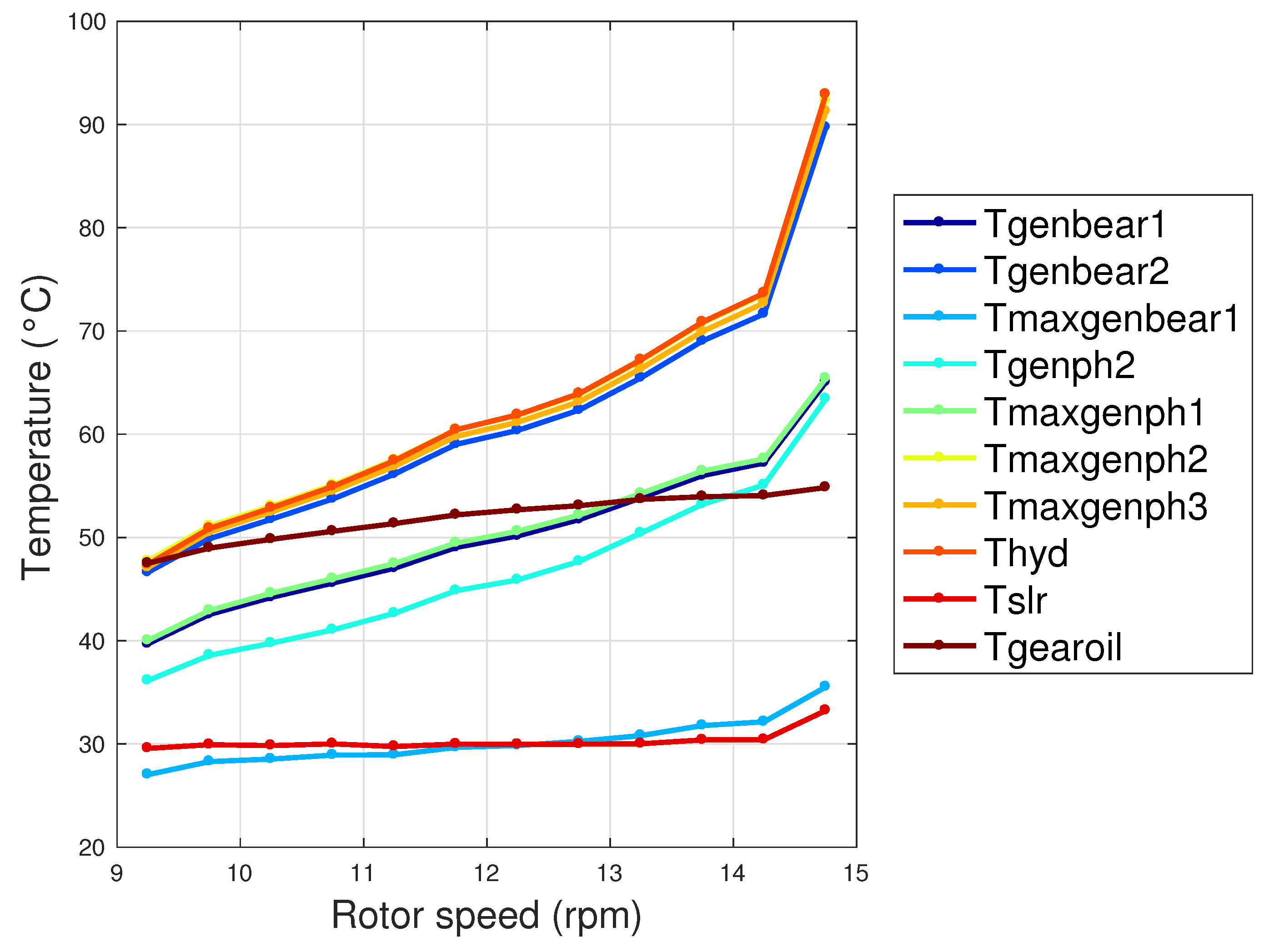
A very interesting aspect is that the support vector regression does not select the rotational speed (rotor or generator), but selects ten temperatures as more meaningful input variables. This is a non-trivial result, because the rotational speed has been considered up to now the most important covariate in addition to the wind speed [19]. This should not lead to diminishing the consideration of the rotational speed as a covariate for wind turbine power curve models, also in light of the fundamental physical meaning of this variable. The message arising from this result is, rather, that the internal temperatures are overlooked for consideration in power curve models. Moreover, a further direction of the present work which is at present being developed regards the use of explainable machine learning methods. An anticipation of the results which are of interest in the present context is that the covariates should be ranked not only by how much the average error diminishes when each covariate is included (as is done in this work), but also for how much the average error (once the set of covariates is selected) depends on each variable. The latter information can be obtained by computing the Shapley coefficients [38,39] for each variable and, for the data sets of this study, the rotational speed ranks as the highest, which means it is the most explanatory. In Table 2, the determination coefficients between the rotor speed and the temperatures selected for the SVR regression are reported. It arises that, for most of the temperatures, such a coefficient is quite high, which explains how it is possible that a purely data-driven model treats as quite interchangeable the rotational speed and the internal temperatures. Finally, an average curve of the selected temperatures as a function of the rotor speed is reported in Figure 2.
A general result arising from Table 1 is that the input variables selected for the two types of regression are different. This further confirms previous results in the literature about the fact that for multivariate wind turbine power curves, one size does not fit all. The selection of the input variables can likely depend on the wind turbine technology [16] and on the type of regression. It is, therefore, very important to start from an appropriately rich data set and to implement rigorous feature selection algorithms.
4.2. Error Metrics
The results for the error metrics of the support vector and Gaussian process regressions are reported in Table 3 as absolute values and normalized to the rated power, as indicated in [17] for convenience of comparison with the literature. In Table 4, the same error metrics are reported for a benchmark which somehow constitutes the standard of multivariate power curve models. Inspired by Equation (1) and by [19,22], the input variables of the benchmark model are wind speed v, blade pitch , and rotational speed .
Comparing Table 3 to Table 4, it arises that for each regression type the models proposed in this work provide error metrics in the order 20–25% lower with respect to the selected benchmark model.
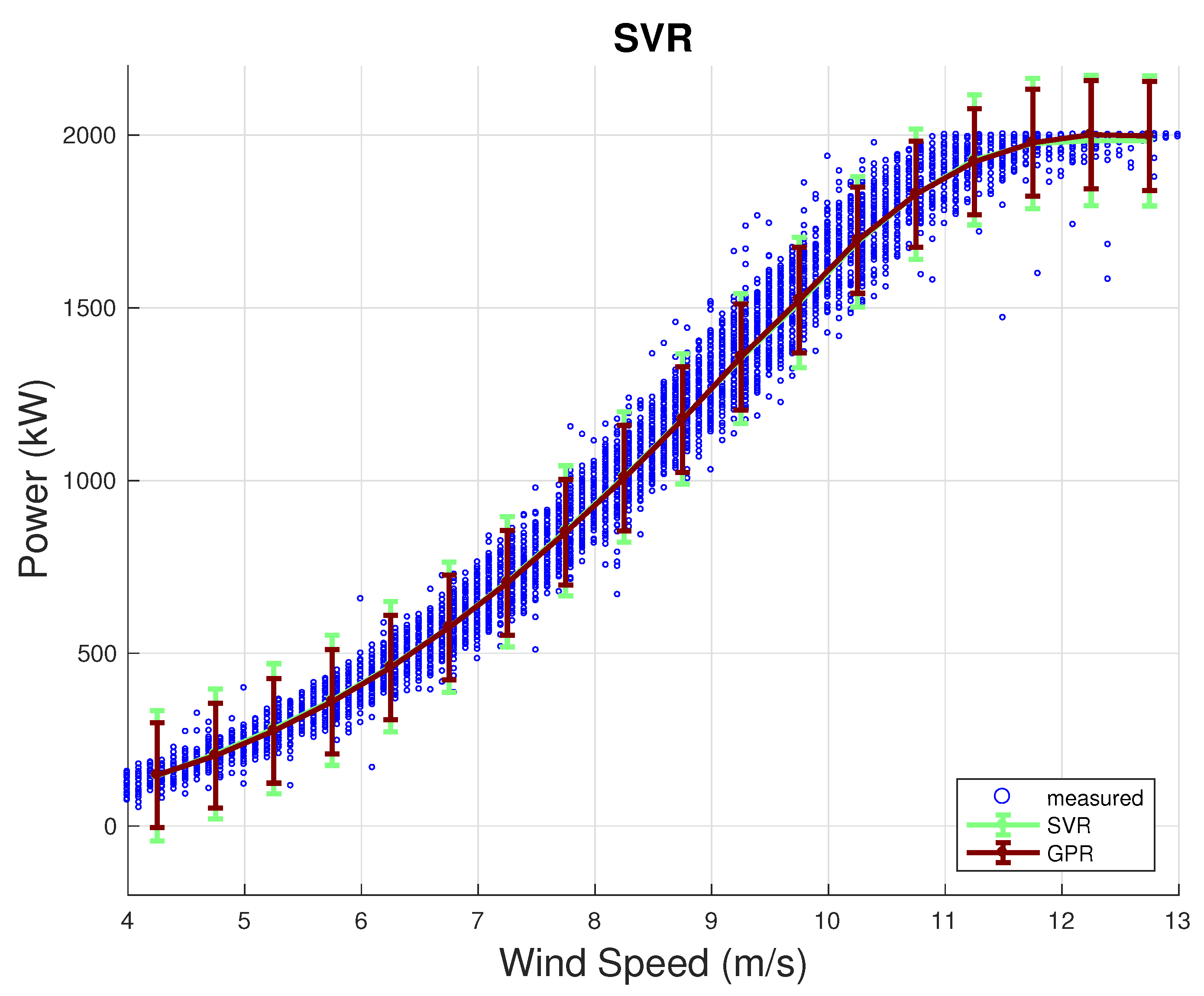
In Figure 3, the measured and simulated power curves are reported, respectively, for the support vector and Gaussian process regressions, with confidence intervals. From this figure, it arises that the proposed models are capable of reproducing very realistically the dispersion of an observed power curve. In the figures, the 95% confidence intervals are reported as well, which for the SVR regression have been computed according to the method indicated in [40].
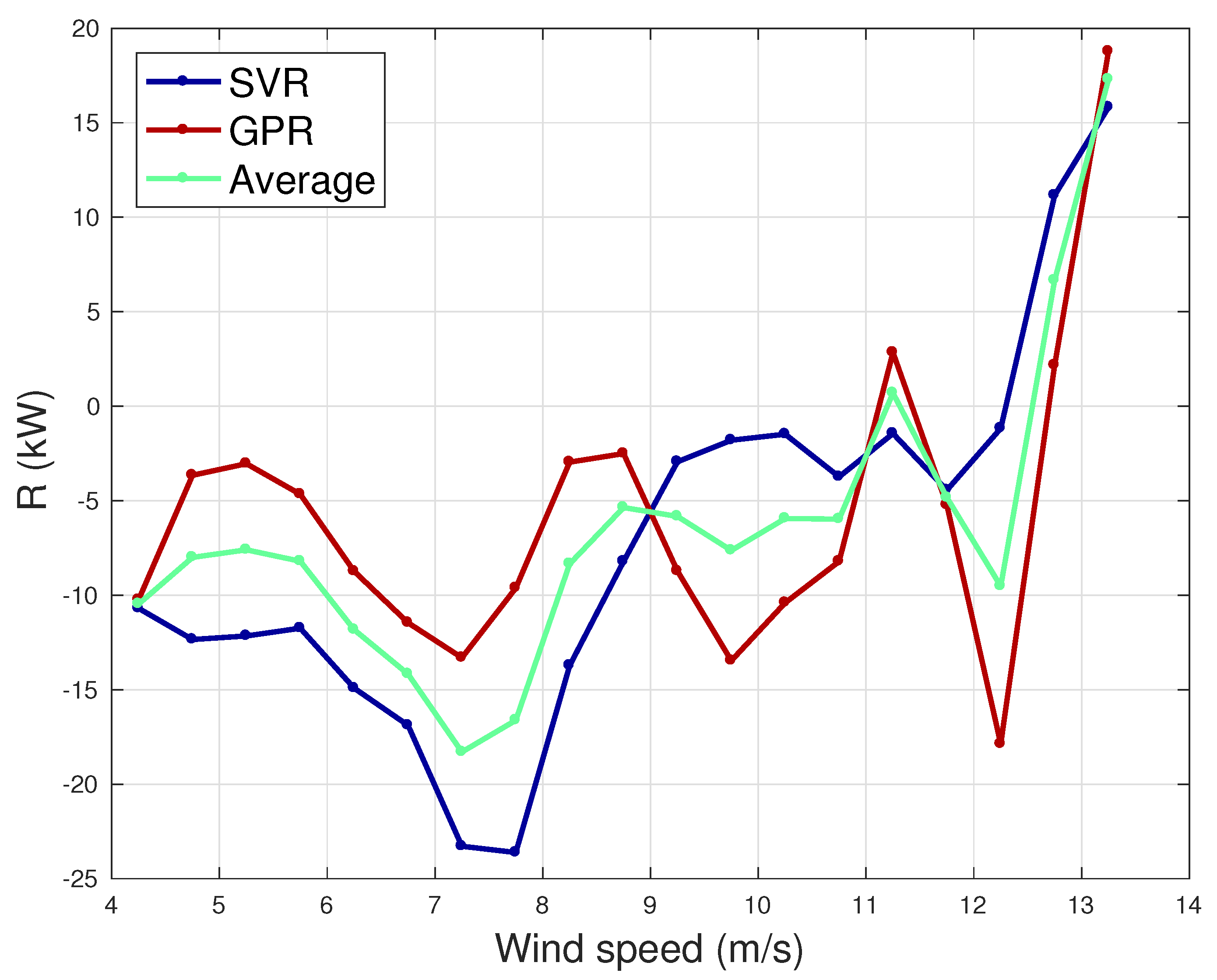
To highlight the differences between the SVR and GPR models, in Figure 4 the residuals R (Equation (20)) have been plotted after averaging per wind speed bins of 0.5 m/s. From this figure, the points of strength of the two regressions can be interpreted in light of the input variables selection of Table 1. The support vector regression displays higher absolute residuals in the regime of variable rotational speed (approximately between 6 and 9 m/s of wind intensity) and this might be due to the fact that the automatic features selection algorithm has excluded the rotational speed, which, in that particular working region of the wind turbine, is very important information. On the other hand, the support vector regression performs better than the Gaussian process regression when approaching the rated speed. This might be due to the fact that the former model employs more temperature covariates, whose behavior increasing with the wind speed is very well correlated with the power. Given these considerations, the average of the estimates provided by the two regressions has also been added in Figure 4. The average of the two estimates provides a slight improvement in the error metrics. Actually, the lowers to 27 kW and the to 37.3 kW. Nevertheless, a more sensible improvement could probably be achieved by customizing the input variables selection depending on the working region of the wind turbines. This could be achieved through data clustering and performing a separate input variables selection for each cluster. Yet, it should be taken into account that separating a data set into clusters leads to dimension reduction of the training data sets for each model in each cluster. Therefore, the estimation of the net balance of this procedure is not straightforward and it is in general important to formulate reliable models spanning all the power curves, as in the present work.
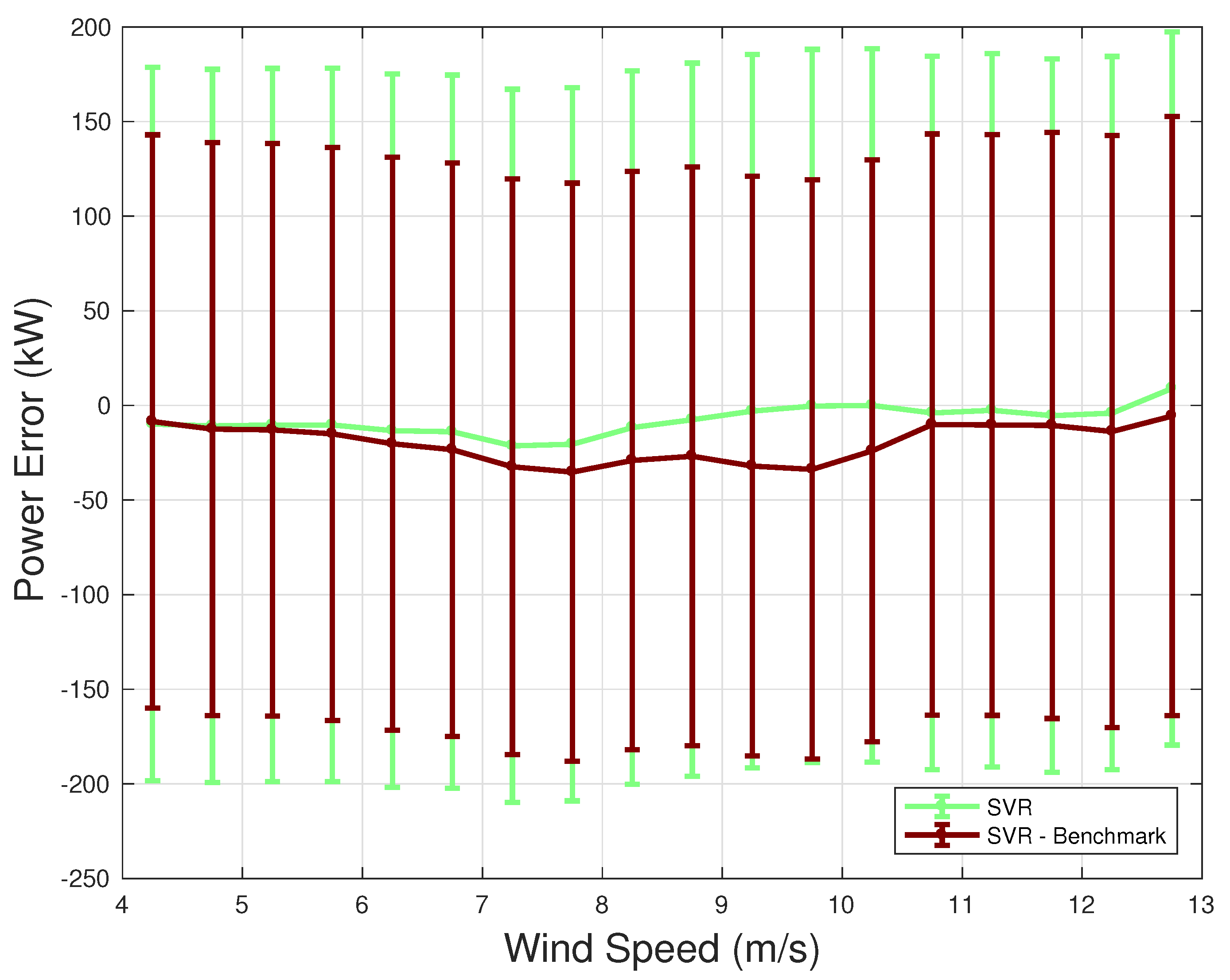
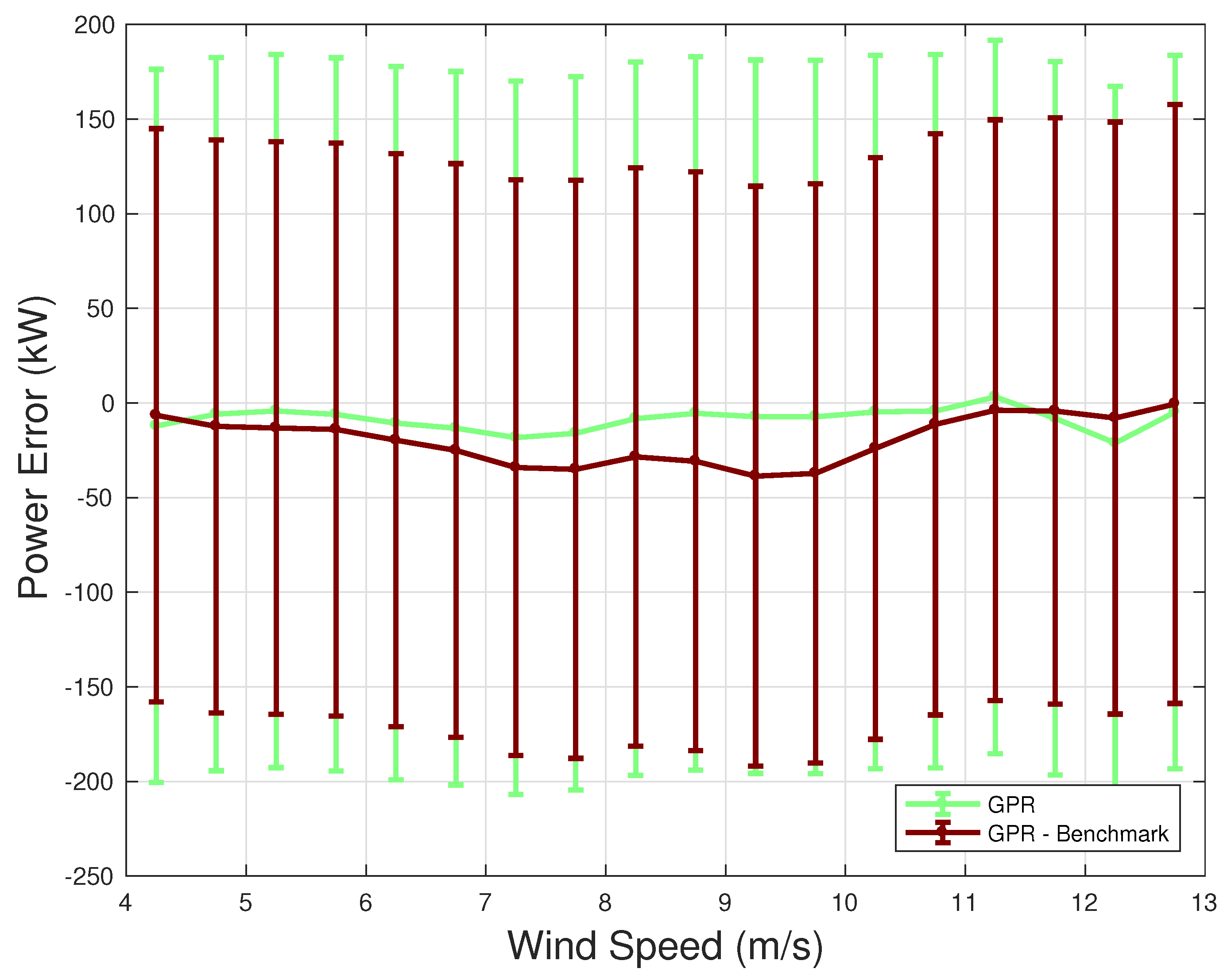
In Figure 5, Figure 6 and Figure 7, the behavior of the selected models is compared against the benchmark ones, which are also compared against themselves. The average difference between measurements and model estimates is reported, with confidence intervals for each model type. From Figure 5 and Figure 6, it arises that the average residuals are closer to zero for the selected models, with respect to their corresponding benchmark. Furthermore, the confidence intervals are noticeably lower. This clearly indicates the advantage of employing a vast set of covariates as a starting point for the model. Finally, it is worth noticing the comparison between the SVR and GPR benchmark models (Figure 7). The situation is qualitatively similar to Figure 4. Depending on the operation regime of the wind turbine, the SVR or GPR regression might be averagely more profitable.
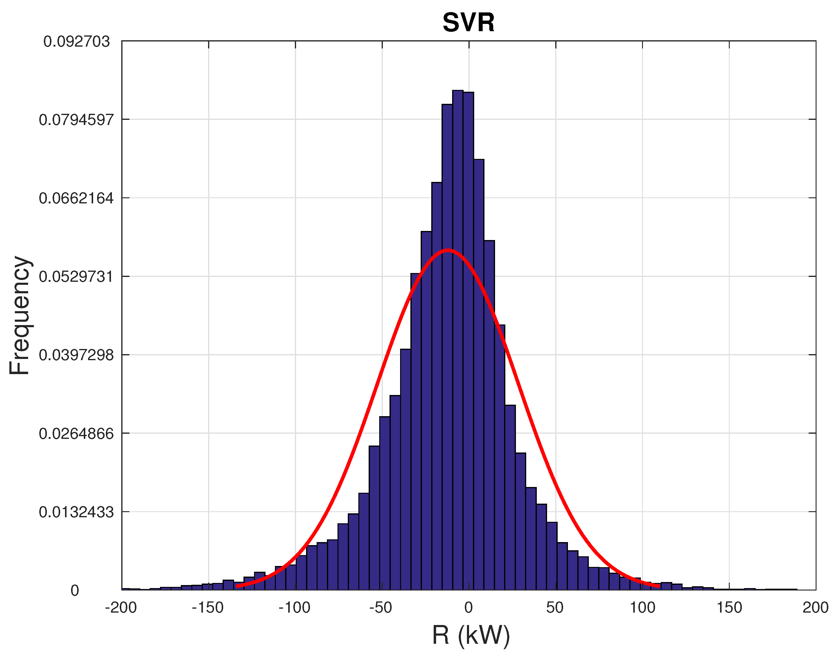
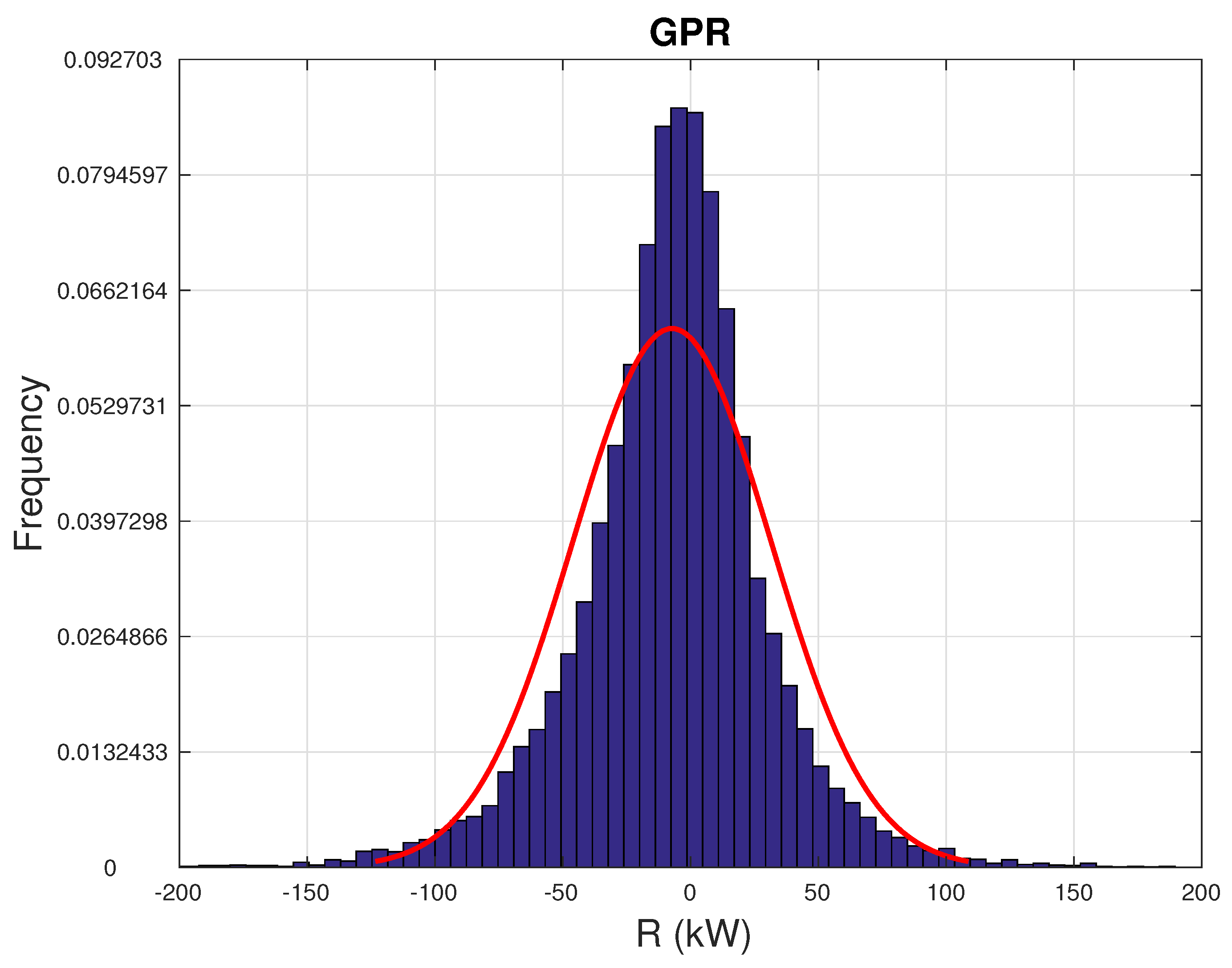
In Figure 8 and Figure 9, the distributions of the residuals R (Equation (20)) are reported, respectively, for the support vector and Gaussian process regressions. In Table 5, the mean, the skewness, and the kurtosis of the residuals are reported for the SVR and GPR regression. It arises that the GPR approximates slightly better a desirable feature of the residuals, which is the symmetry, but there is a little higher probability of having a very abnormal absolute residual (due to the higher kurtosis with respect to SVR). This once again confirms that it is over-optimistic to have all the desirable features in the same model and that a combination of several model estimates, although non-trivial to obtain, might improve the performance. For both models, the kurtosis of the residuals is largely higher than the Gaussian distribution, which means that there is a relatively high probability of having a large mismatch between measurement and model estimate.
4.3. Application for Anomaly Detection
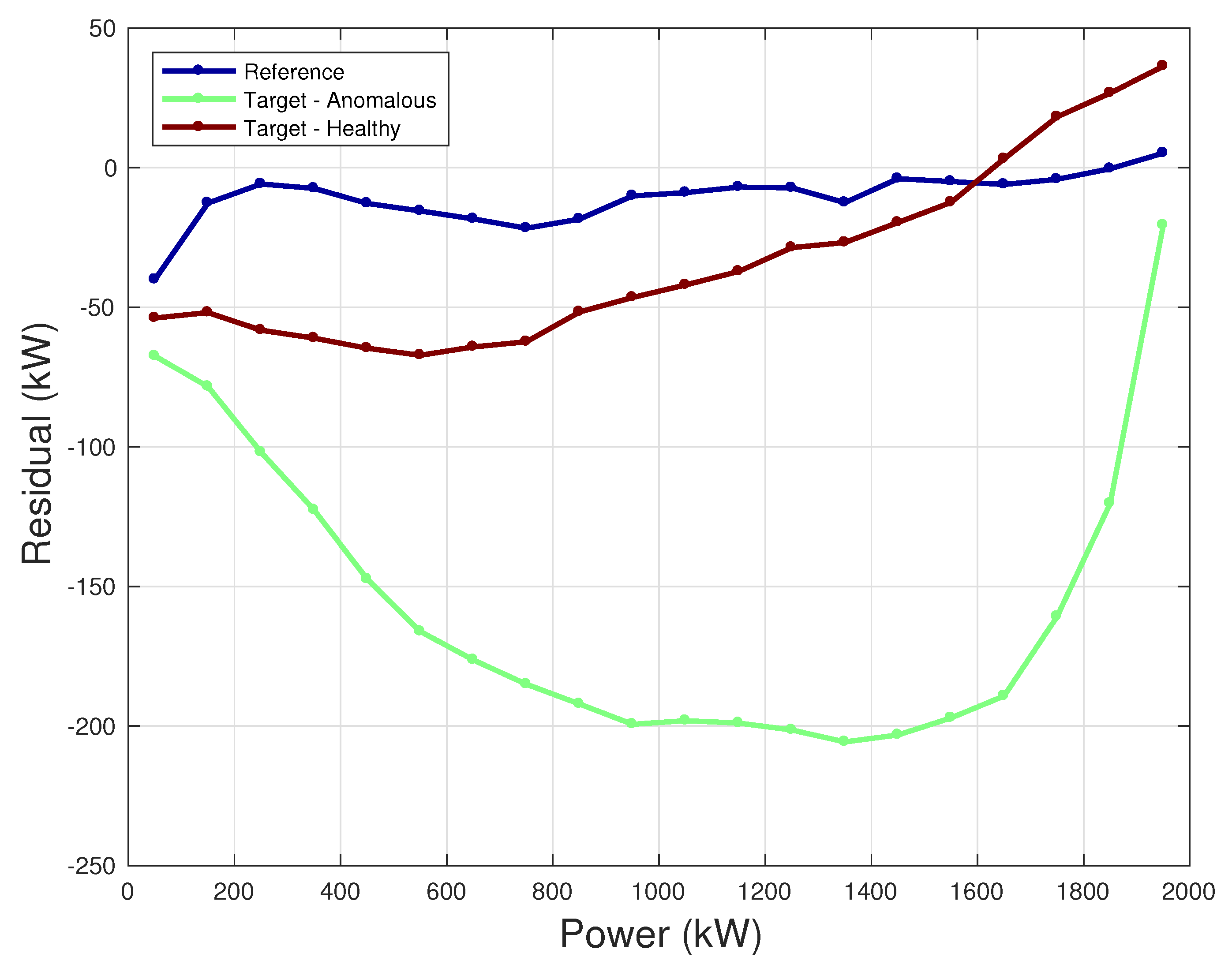
The application of the proposed method for the prognosis of incoming faults requires devoted techniques, which represent the future directions of this work and deserve a detailed discussion. For the purposes of this study, it is interesting to report a brief example of an application for the identification of an overall anomaly (related to the rotor) affecting the functioning of a wind turbine from the same farm. The idea is simulating the power of the target wind turbines using the model developed for the reference wind turbine, details of which are reported in Section 4.1 and Section 4.2. For this example, we select as target wind turbines the anomalous one and a healthy one and we highlight the difference between the two sets of residuals.
From Figure 10, it arises that if one employs the model trained with the data of the reference wind turbine, the residuals are largely negative for the target anomalous wind turbine, which means underperformance. A very slight underperformance can also be hypothesized for the target healthy wind turbine, but it should be noticed that the curves for the healthy wind turbines are surely compatible with the confidence intervals (which have not been reported merely for clarity of the figure) and also within the reported in Table 3, different with respect to what happens between the reference wind turbine and the target anomalous wind turbine.
5. Conclusions and Further Directions
The present study has been devoted to the analysis of multivariate data-driven models for the power curve of wind turbines. As discussed in Section 1, this subject has been recently attracting remarkable attention in the wind energy literature, but there are several qualifying points which are left to the scholar’s discretion, which substantially are the selection of the model type and of the input variables.
For this reason, in this work, two types of regression (support vector and Gaussian process) have been applied to a real-world test case, based on the data of a 2 MW wind turbine owned by ENGIE Italia. The most innovative aspect of this study is that several sub-component temperatures have been included as potential covariates of the model. Actually, at present, in the literature the additional covariates which have been mostly employed are rotational speed and blade pitch, but there is no conceptual reason why the vast set of temperature sensors with which a wind turbine is equipped should not be used for this kind of purpose.
The above idea has been corroborated by the results achieved in this study. A sequential features selection, based on the objective of loss minimization through 10-fold cross-validation, abundantly selects the temperatures which have been included as potential covariates. As expected, a slightly different input variables selection is achieved for the two regression types. This supports the goodness of the use of an automatic features selection, because the selected set could not be individuated by straightforward intuition. In summary, the main practical result of the present study is that the proposed models, when validated to simulate the output on an out-of-sample data set, provide average error metrics which are in the order of 20–25% lower with respect to a benchmark model which can be considered the standard in multivariate wind turbine power curve analysis. An example of a practical application of the proposed method is discussed, which deals with the identification of underperformance through a space-time comparison [41]. The data-driven model is trained with the data of a reference wind turbine and, once the power of target wind turbines is simulated, the properties of the residuals are analyzed.
As supported in Section 1, it should be noticed that the improvement achieved by including sub-component temperatures in multivariate power curves is not only a matter of diminishing the error metrics, which means increasing the capability of the model in capturing the normal behavior of the machine. Potentially, the use of sub-component temperatures in multivariate wind turbine power curves involves developments in condition monitoring. Actually, sub-component temperatures of wind turbines are widely employed for detecting faults, because a common manifestation of incoming damages is anomalous heating and a slight decrease of the extracted power [27,28]. In this regard, there are several possible approaches. In case of non-labeled data, the idea for regression-based condition monitoring is modeling the normal behavior of the component temperature of interest and raising an alarm when the residual between measurement and model estimate exceeds a certain threshold [42,43]. Classification methods are widely employed as well, as in [44,45], for the diagnosis of generator faults. When labeled data are available, the typical critical point is that they are highly imbalanced because, hopefully, a wind turbine has been operating in a healthy state most of the time. This calls for devoted techniques, such as the so-called few-shot learning [46].
In this context, the multivariate regressions proposed in this study combine the input (wind intensity), the main operation variables (such as rotational speed or blade pitch), and the internal temperatures to predict the normal-behavior model estimate for the power of a wind turbine and, in principle, have a superior potentiality for identifying anomalies in the form of the increased residual between measurements and model estimates. This is the main further direction of the present work, which is at its early stages in the literature but has already proved to be promising [47,48,49].
Another challenge given by the fact that wind energy is projected into the era of big data [50] is understanding how scalable the employed methods are. The implicit assumption of the method proposed in this work is that a data-driven model has to be trained for each monitored wind turbine and this increases the computational cost when the number of wind turbines increases. First developments have been achieved [51] for the analysis of how big the training data set should be and how the thresholds for alarm raising should be defined, depending on the requested statistical significance (which in turn means computational cost). A deeper investigation of this point should be pursued, for example by formulating methods for limiting the number of models to be trained as much as possible, without losing too much statistical significance.
Author Contributions
Conceptualization, D.A., R.P., A.L. and L.T.; methodology, D.A. and R.P.; software, D.A. and R.P.; validation, D.A.; formal analysis, D.A. and R.P.; investigation, D.A., R.P. and A.L.; resources, A.L. and L.T.; data curation, D.A. and A.L.; writing—original draft preparation, D.A.; writing—review and editing, R.P., A.L. and L.T.; visualization, D.A., R.P. and L.T.; supervision, L.T.; project administration, L.T. All authors have read and agreed to the published version of the manuscript.
Funding
The authors declare no external funding.
Conflicts of Interest
The authors declare no conflict of interest.
References
- Ackermann, T. Wind Power in Power Systems; John Wiley & Sons: Hoboken, NJ, USA, 2005. [Google Scholar]
- Astolfi, D.; Pandit, R.; Terzi, L.; Lombardi, A. Discussion of wind turbine performance based on SCADA data and multiple test case analysis. Energies 2022, 15, 5343. [Google Scholar] [CrossRef]
- Honrubia, A.; Vigueras-Rodríguez, A.; Gómez-Lázaro, E. The influence of turbulence and vertical wind profile in wind turbine power curve. In Progress in Turbulence and Wind Energy IV; Springer: Berlin, Germany, 2012; pp. 251–254. [Google Scholar]
- Hedevang, E. Wind turbine power curves incorporating turbulence intensity. Wind Energy 2014, 17, 173–195. [Google Scholar] [CrossRef]
- Pandit, R.K.; Infield, D.; Carroll, J. Incorporating air density into a Gaussian process wind turbine power curve model for improving fitting accuracy. Wind Energy 2019, 22, 302–315. [Google Scholar] [CrossRef] [Green Version]
- Wang, Y.; Hu, Q.; Li, L.; Foley, A.M.; Srinivasan, D. Approaches to wind power curve modeling: A review and discussion. Renew. Sustain. Energy Rev. 2019, 116, 109422. [Google Scholar] [CrossRef]
- Ciulla, G.; D’Amico, A.; Di Dio, V.; Brano, V.L. Modelling and analysis of real-world wind turbine power curves: Assessing deviations from nominal curve by neural networks. Renew. Energy 2019, 140, 477–492. [Google Scholar] [CrossRef]
- Butler, S.; Ringwood, J.; O’Connor, F. Exploiting SCADA system data for wind turbine performance monitoring. In Proceedings of the 2013 Conference on Control and Fault-Tolerant Systems (SysTol), Nice, France, 9–11 October 2013; pp. 389–394. [Google Scholar]
- Long, H.; Wang, L.; Zhang, Z.; Song, Z.; Xu, J. Data-driven wind turbine power generation performance monitoring. IEEE Trans. Ind. Electron. 2015, 62, 6627–6635. [Google Scholar] [CrossRef]
- Gonzalez, E.; Stephen, B.; Infield, D.; Melero, J.J. Using high-frequency SCADA data for wind turbine performance monitoring: A sensitivity study. Renew. Energy 2019, 131, 841–853. [Google Scholar] [CrossRef] [Green Version]
- Astolfi, D.; Castellani, F.; Terzi, L. Mathematical methods for SCADA data mining of onshore wind farms: Performance evaluation and wake analysis. Wind Eng. 2016, 40, 69–85. [Google Scholar] [CrossRef] [Green Version]
- Theodorakatos, N.P.; Lytras, M.; Babu, R. Towards smart energy grids: A box-constrained nonlinear underdetermined model for power system observability using recursive quadratic programming. Energies 2020, 13, 1724. [Google Scholar] [CrossRef] [Green Version]
- Theodorakatos, N.P.; Lytras, M.; Babu, R. A generalized pattern search algorithm methodology for solving an under-determined system of equality constraints to achieve power system observability using synchrophasors. J. Phys. Conf. Ser. 2021, 2090, 012125. [Google Scholar] [CrossRef]
- Vide, P.S.C.; Barbosa, F.M.; Ferreira, I.M. Combined use of SCADA and PMU measurements for power system state estimator performance enhancement. In Proceedings of the 2011 3rd International Youth Conference on Energetics (IYCE), Leiria, Portugal, 7–9 July 2011; pp. 1–6. [Google Scholar]
- Vanfretti, L.; Baudette, M.; Domínguez-García, J.L.; Almas, M.S.; White, A.; Gjerde, J.O. A phasor measurement unit based fast real-time oscillation detection application for monitoring wind-farm-to-grid sub–synchronous dynamics. Electr. Power Compon. Syst. 2016, 44, 123–134. [Google Scholar] [CrossRef] [Green Version]
- Astolfi, D.; Castellani, F.; Lombardi, A.; Terzi, L. Multivariate SCADA data analysis methods for real-world wind turbine power curve monitoring. Energies 2021, 14, 1105. [Google Scholar] [CrossRef]
- Astolfi, D. Perspectives on SCADA Data Analysis Methods for Multivariate Wind Turbine Power Curve Modeling. Machines 2021, 9, 100. [Google Scholar] [CrossRef]
- Janssens, O.; Noppe, N.; Devriendt, C.; Van de Walle, R.; Van Hoecke, S. Data-driven multivariate power curve modeling of offshore wind turbines. Eng. Appl. Artif. Intell. 2016, 55, 331–338. [Google Scholar] [CrossRef]
- Pandit, R.K.; Infield, D.; Kolios, A. Gaussian process power curve models incorporating wind turbine operational variables. Energy Rep. 2020, 6, 1658–1669. [Google Scholar] [CrossRef]
- Shetty, R.P.; Sathyabhama, A.; Pai, P.S. Comparison of modeling methods for wind power prediction: A critical study. Front. Energy 2020, 14, 347–358. [Google Scholar] [CrossRef]
- Karamichailidou, D.; Kaloutsa, V.; Alexandridis, A. Wind turbine power curve modeling using radial basis function neural networks and tabu search. Renew. Energy 2021, 163, 2137–2152. [Google Scholar] [CrossRef]
- Astolfi, D.; Castellani, F.; Natili, F. Wind Turbine Multivariate Power Modeling Techniques for Control and Monitoring Purposes. J. Dyn. Syst. Meas. Control 2021, 143, 034501. [Google Scholar] [CrossRef]
- Niu, W.; Huang, J.; Yang, H.; Wang, X. Wind turbine power prediction based on wind energy utilization coefficient and multivariate polynomial regression. J. Renew. Sustain. Energy 2022, 14, 013306. [Google Scholar] [CrossRef]
- Jing, H.; Zhao, C. Adjustable piecewise regression strategy based wind turbine power forecasting for probabilistic condition monitoring. Sustain. Energy Technol. Assess. 2022, 52, 102013. [Google Scholar] [CrossRef]
- Marčiukaitis, M.; Žutautaitė, I.; Martišauskas, L.; Jokšas, B.; Gecevičius, G.; Sfetsos, A. Non-linear regression model for wind turbine power curve. Renew. Energy 2017, 113, 732–741. [Google Scholar] [CrossRef]
- Rabanal, A.; Ulazia, A.; Ibarra-Berastegi, G.; Sáenz, J.; Elosegui, U. MIDAS: A benchmarking multi-criteria method for the identification of defective anemometers in wind farms. Energies 2019, 12, 28. [Google Scholar] [CrossRef] [Green Version]
- Zaher, A.; McArthur, S.; Infield, D.; Patel, Y. Online wind turbine fault detection through automated SCADA data analysis. Wind Energy Int. J. Prog. Appl. Wind Power Convers. Technol. 2009, 12, 574–593. [Google Scholar] [CrossRef]
- Corley, B.; Koukoura, S.; Carroll, J.; McDonald, A. Combination of thermal modelling and machine learning approaches for fault detection in wind turbine gearboxes. Energies 2021, 14, 1375. [Google Scholar] [CrossRef]
- Barber, S.; Nordborg, H. Improving site-dependent power curve prediction accuracy using regression trees. J. Phys. Conf. Ser. 2020, 1618, 062003. [Google Scholar] [CrossRef]
- Barber, S.; Hammer, F.; Tica, A. Improving Site-Dependent Wind Turbine Performance Prediction Accuracy Using Machine Learning. ASCE-ASME J. Risk Uncertain. Eng. Syst. Part B Mech. Eng. 2022, 8, 021102. [Google Scholar] [CrossRef]
- Astolfi, D.; Castellani, F.; Becchetti, M.; Lombardi, A.; Terzi, L. Wind Turbine Systematic Yaw Error: Operation Data Analysis Techniques for Detecting It and Assessing Its Performance Impact. Energies 2020, 13, 2351. [Google Scholar] [CrossRef]
- Astolfi, D.; Pandit, R.; Gao, L.; Hong, J. Individuation of Wind Turbine Systematic Yaw Error through SCADA Data. Energies 2022, 15, 8165. [Google Scholar] [CrossRef]
- Carullo, A.; Ciocia, A.; Di Leo, P.; Giordano, F.; Malgaroli, G.; Peraga, L.; Spertino, F.; Vallan, A. Comparison of correction methods of wind speed for performance evaluation of wind turbines. In Proceedings of the 24th IMEKO-TC4 International Symposium, Palermo, Italy, 14–16 September 2020; pp. 291–296. [Google Scholar]
- Carullo, A.; Ciocia, A.; Malgaroli, G.; Spertino, F. An Innovative Correction Method of Wind Speed for Efficiency Evaluation of Wind Turbines. Acta IMEKO 2021, 10, 46–53. [Google Scholar] [CrossRef]
- De Caro, F.; Vaccaro, A.; Villacci, D. Adaptive wind generation modeling by fuzzy clustering of experimental data. Electronics 2018, 7, 47. [Google Scholar] [CrossRef]
- Pandit, R.K.; Infield, D. Comparative assessments of binned and support vector regression-based blade pitch curve of a wind turbine for the purpose of condition monitoring. Int. J. Energy Environ. Eng. 2019, 10, 181–188. [Google Scholar] [CrossRef] [Green Version]
- Rasmussen, C.E. Gaussian processes in machine learning. In Proceedings of the Summer School on Machine Learning, Canberra, Australia, 2–14 February 2003; pp. 63–71. [Google Scholar]
- Pang, C.; Yu, J.; Liu, Y. Correlation analysis of factors affecting wind power based on machine learning and Shapley value. IET Energy Syst. Integr. 2021, 3, 227–237. [Google Scholar] [CrossRef]
- Zhang, J.; Liu, D.; Li, Z.; Han, X.; Liu, H.; Dong, C.; Wang, J.; Liu, C.; Xia, Y. Power prediction of a wind farm cluster based on spatiotemporal correlations. Appl. Energy 2021, 302, 117568. [Google Scholar] [CrossRef]
- Pandit, R.; Kolios, A. SCADA data-based support vector machine wind turbine power curve uncertainty estimation and its comparative studies. Appl. Sci. 2020, 10, 8685. [Google Scholar] [CrossRef]
- Ding, Y.; Kumar, N.; Prakash, A.; Kio, A.E.; Liu, X.; Liu, L.; Li, Q. A case study of space-time performance comparison of wind turbines on a wind farm. Renew. Energy 2021, 171, 735–746. [Google Scholar] [CrossRef]
- Encalada-Dávila, Á.; Moyón, L.; Tutivén, C.; Puruncajas, B.; Vidal, Y. Early fault detection in the main bearing of wind turbines based on Gated Recurrent Unit (GRU) neural networks and SCADA data. IEEE/ASME Trans. Mechatron. 2022, 27, 5583–5593. [Google Scholar] [CrossRef]
- Xiang, L.; Wang, P.; Yang, X.; Hu, A.; Su, H. Fault detection of wind turbine based on SCADA data analysis using CNN and LSTM with attention mechanism. Measurement 2021, 175, 109094. [Google Scholar] [CrossRef]
- Jin, X.; Xu, Z.; Qiao, W. Condition monitoring of wind turbine generators using SCADA data analysis. IEEE Trans. Sustain. Energy 2020, 12, 202–210. [Google Scholar] [CrossRef]
- Peter, R.; Zappalá, D.; Schamboeck, V.; Watson, S.J. Wind turbine generator prognostics using field SCADA data. J. Phys. Conf. Ser. 2022, 2265, 032111. [Google Scholar] [CrossRef]
- Liu, X.; Teng, W.; Liu, Y. A Model-Agnostic Meta-Baseline Method for Few-Shot Fault Diagnosis of Wind Turbines. Sensors 2022, 22, 3288. [Google Scholar] [CrossRef]
- Castellani, F.; Astolfi, D.; Natili, F. SCADA data analysis methods for diagnosis of electrical faults to wind turbine generators. Appl. Sci. 2021, 11, 3307. [Google Scholar] [CrossRef]
- Zhao, Y.; Li, D.; Dong, A.; Kang, D.; Lv, Q.; Shang, L. Fault prediction and diagnosis of wind turbine generators using SCADA data. Energies 2017, 10, 1210. [Google Scholar] [CrossRef] [Green Version]
- Wei, L.; Qian, Z.; Zareipour, H.; Zhang, F. Comprehensive aging assessment of pitch systems combining SCADA and failure data. IET Renew. Power Gener. 2022, 16, 198–210. [Google Scholar] [CrossRef]
- Ding, Y. Data Science for Wind Energy; CRC Press: Boca Raton, FL, USA, 2019. [Google Scholar]
- Turnbull, A.; Carroll, J.; McDonald, A. A comparative analysis on the variability of temperature thresholds through time for wind turbine generators using normal behaviour modelling. Energies 2022, 15, 5298. [Google Scholar] [CrossRef]
Figure 1.
An example of scattered power curve before and after data pre-processing.

Figure 2.
Average curve of the internal temperatures selected by the SVR regression as a function of the rotor speed .
Figure 2.
Average curve of the internal temperatures selected by the SVR regression as a function of the rotor speed .

Figure 3.
Measured and simulated power curve (SVR and GPR), with confidence intervals.

Figure 4.
Residuals of the SVR and GPR, averaged per wind speed bins of 0.5 m/s.

Figure 5.
Average error between model predictions and model estimate: SVR and SVR benchmark.

Figure 6.
Average error between model predictions and model estimate: GPR and GPR benchmark.

Figure 7.
Average error between model predictions and model estimate: SVR benchmark and GPR benchmark.
Figure 7.
Average error between model predictions and model estimate: SVR benchmark and GPR benchmark.

Figure 8.
Histogram of the residuals R between measurements and SVR model estimates.

Figure 9.
Histogram of the residuals R between measurements and GPR model estimates.

Figure 10.
Residuals between measurements and model estimates as a function of the measured power: reference wind turbine, target anomalous, and target health.
Figure 10.
Residuals between measurements and model estimates as a function of the measured power: reference wind turbine, target anomalous, and target health.


Table 1.
Input variables selection for the SVR and GPR and coefficient of determination with the power P.
Table 1.
Input variables selection for the SVR and GPR and coefficient of determination with the power P.
| Model | Selected Input Variables | |
|---|---|---|
| SVR | v, , , , , , , , , , , | (0.98, 0.48, 0.76, 0.87, 0.44, 0.76, 0.76, 0.88, 0.88, 0.88, 0.26, 0.55) |
| GPR | v, , , , , , , | (0.98, 0.85, 0.48, 0.76, 0.44, 0.76, 0.76, 0.88, 0.26) |
Table 2.
Coefficient of determination between the internal temperatures selected for the SVR regression and the rotor speed .
Table 2.
Coefficient of determination between the internal temperatures selected for the SVR regression and the rotor speed .
| Model | Selected Temperatures | |
|---|---|---|
| SVR | , , , , , , , , , | (0.75, 0.77, 0.48, 0.75, 0.75 0.78, 0.78, 0.78, 0.25, 0.69) |
Table 3.
Error metrics for the SVR and GPR validation.
| Model | (kW) | (kW) | (%) | (%) |
|---|---|---|---|---|
| SVR | 29.6 | 40.7 | 1.48 | 2.03 |
| GPR | 27.7 | 38.7 | 1.35 | 1.94 |
Table 4.
Error metrics for the SVR and GPR validation for the benchmark model.
| Model | (kW) | (kW) | (%) | (%) |
|---|---|---|---|---|
| SVR—Benchmark | 35.7 | 48.3 | 1.79 | 2.41 |
| GPR—Benchmark | 36.5 | 48.5 | 1.82 | 2.43 |
Table 5.
Statistical properties of the residuals between measurements and model estimates.
| Model | Mean (kW) | Skewness | Kurtosis |
|---|---|---|---|
| SVR | −7.2 | −0.41 | 9.36 |
| GPR | −5.4 | −0.36 | 9.54 |
Disclaimer/Publisher’s Note: The statements, opinions and data contained in all publications are solely those of the individual author(s) and contributor(s) and not of MDPI and/or the editor(s). MDPI and/or the editor(s) disclaim responsibility for any injury to people or property resulting from any ideas, methods, instructions or products referred to in the content. |
© 2022 by the authors. Licensee MDPI, Basel, Switzerland. This article is an open access article distributed under the terms and conditions of the Creative Commons Attribution (CC BY) license (https://creativecommons.org/licenses/by/4.0/).
Share and Cite
MDPI and ACS Style
Astolfi, D.; Pandit, R.; Lombardi, A.; Terzi, L. Multivariate Data-Driven Models for Wind Turbine Power Curves including Sub-Component Temperatures. Energies 2023, 16, 165. https://0-doi-org.brum.beds.ac.uk/10.3390/en16010165
AMA Style
Astolfi D, Pandit R, Lombardi A, Terzi L. Multivariate Data-Driven Models for Wind Turbine Power Curves including Sub-Component Temperatures. Energies. 2023; 16(1):165. https://0-doi-org.brum.beds.ac.uk/10.3390/en16010165
Chicago/Turabian StyleAstolfi, Davide, Ravi Pandit, Andrea Lombardi, and Ludovico Terzi. 2023. "Multivariate Data-Driven Models for Wind Turbine Power Curves including Sub-Component Temperatures" Energies 16, no. 1: 165. https://0-doi-org.brum.beds.ac.uk/10.3390/en16010165
Note that from the first issue of 2016, this journal uses article numbers instead of page numbers. See further details here.