
Multicriteria Design and Operation Optimization of a Solar-Assisted Geothermal Heat Pump System


1
Mechanical Engineering Department, University of Western Macedonia, Kozani 50100, Greece
2
Electrical and Computer Engineering Department, University of Western Macedonia, Kozani 50100, Greece
*
Author to whom correspondence should be addressed.
Energies 2023, 16(3), 1266; https://0-doi-org.brum.beds.ac.uk/10.3390/en16031266
Submission received: 23 December 2022
/
Revised: 16 January 2023
/
Accepted: 23 January 2023
/
Published: 25 January 2023
(This article belongs to the Special Issue Advances in Solar Thermal Energy Storage Technologies)
Abstract
:This work focuses on the determination of the design and operation parameters of a thermal system depending on the optimization objective set. Its main objective and contribution concern the proposal of a generalized methodological structure involving multiobjective optimization techniques aimed at providing a solution to a practical problem, such as the design and dimensioning of a solar thermal system. The analysis is based on system operation data provided by a dynamic simulation model, leading to the development of multiple surrogate models of the thermal system. The thermal system surrogate models correlate the desired optimization objectives with thermal system design and operation parameters while additional surrogate models of the Pareto frontiers are generated. The implementation of the methodology is demonstrated through the optimal design and operation parameter dimensioning of a solar-assisted geothermal heat pump that provides domestic hot water loads of an office building. Essentially, energy consumption is optimized for a desired domestic hot water thermal load coverage. Implementation of reverse-engineering methods allows the determination of the system parameters representing the optimized criteria.
1. Introduction
1.1. State of the Art
In recent years, the building energy consumption has been known to amount to a substantial portion of the total primary energy consumption [1]. As it has been established that HVAC systems contribute significantly to the phenomenon [2], dimensioning methodologies have been applied for the reduction of energy consumed by buildings, such as the standards produced by ASHRAE [3,4] regarding building energy efficiency and the European directives regarding building energy performance [5]. Apart from the theoretical dimensioning approaches, research has been focusing on extracting building thermal system dimensioning directives using system simulation models. Despite their ability to identify personalized features of heating, ventilation, and air conditioning (HVAC) systems, simulation models are also accompanied by complex structures for effective thermal mechanics implementation. This in turn leads to considerable computational power [6]. Some studies have looked into this matter. For example, [7] produced a compact physical model for simulating fluid and thermal dynamics in district heating networks at a reduced computational cost; another similar approach was adopted by [8].
Surrogate models [9] are a simplified alternative to system simulation models that also possess satisfactory accuracy. In short, they are a great tool to be used for addressing the shortcomings of the more sophisticated simulation models mentioned above. Several works have used surrogate modeling to focus on control strategy implementation. More specifically, [10] implemented model predictive control to achieve HVAC energy reduction and comfort maintenance of an office building by controlling optimization. The same objectives were realized by [11] by implementing reinforcement learning. While [12] also used reinforcement learning, the optimization objectives focused on energy cost savings in the presence of time-varying electricity prices. In the work of [13], another variant of the predictive controlling modeling structure was proposed, which strives for minimization of energy consumption and discomfort of an office building. Finally, [14] proposed a hierarchical control for power use optimization while being subjected to inherent HVAC and comfort limitations. Surrogate modeling can also be seen in building thermal load prediction applications [15].
Regarding building and HVAC dimensioning decision tools, various works can be found in the literature. More particularly, [16] proposed a decision-making support methodology for district heating system retrofitting. This work had an expansive set of optimization actions but lacked detailed information of the final design parameter that should be implemented in the optimal solutions. The authors of [17] used particle swarm optimization to find the optimal set of district heating network length and consumer number while targeting minimized life cycle cost. The authors of [18] proposed an optimization methodology for the design and control of smart glazed windows. Lastly, [19] developed a surrogate model structure based on mixed integer linear programming. The model provides optimal heating and cooling power for different technologies in buildings that belong to a distributed energy network for several design scenarios. The optimization objective is the minimization of the total network annualized cost. Surrogate modeling can be found even in cases of controlling or dimensioning components of a thermal system using dynamic simulations, such as in [20], where the operation setpoints of a HP was optimized for different thermal storage sizes, or in [21], which used the optimal heating storage size for peak load reduction purposes. What can be inferred from the above works is that there are multiple approaches for effective controlling and dimensioning for large-scale applications that focus on general parameters such as system thermal power. However, aside from a few case studies, generalized methodologies for optimizing individual parameters from various components in a thermal load consumption structure are limited.
While surrogate modeling has been widely used for predicting building loads and has become a vital tool to optimize HVAC controlling, the same cannot be said for HVAC optimized design and operation solutions. There are retrofitting cases, although only a few following cases systematize their approach to a methodology context.
A more specific aspect of HVAC optimization through surrogate modeling lies in multiobjective optimization (MOO). According to [22] “multi-objective optimization has been applied to many fields of science, including engineering, where optimal decisions need to be taken in the presence of trade-offs between two or more objectives that may be in conflict”. While the limitations of [16] have already been outlined, it is important to note that the aforementioned work also contained a MOO structure. An interesting surrogate retrofit model for buildings and thermal systems was proposed by [23] for optimizing the environmental footprint of building energy systems as well as their annual cost. The proposed surrogate model consisted of two machine-learning submodels and performed MOO, providing retrofitting solutions to residential buildings. In the work of [24], a solar-assisted heat pump HP was optimized in terms of thermal comfort in a swimming pool as well as its annual life cycle cost. The authors of [25] performed MOO in a district heating and cooling system for an annual time horizon using hourly simulation data. The above research revealed that different objective sets led to different dimensioning options, which also changed depending on the controlling strategies used. Moreover, it was shown that MOO could be implemented on a larger optimization scale than two objectives [26]. However, a generalized MOO methodology context is necessary to encourage this approach.
In several approaches where multiobjective optimization is employed, retrofitting options are based on specific scenarios and not open-ended parameterization of thermal system components, as observed in [27,28]. In addition, from the works above as well as from [29], it can be seen that the focus is on either design variables or operation-controlling variable optimization and not on both simultaneously. Concerning the above, it would be intriguing to implement a methodology that takes any component parameter as an input, for example, a design parameter, such as nominal power of a HP or storage tank capacity, and at the same time an operation parameter, such as temperature setpoints or thermal loop mass supply.
The literature has been focused on producing surrogate models that are suitable for performing retrofitting and controlling optimization. Most works provide general optimization solutions on large-scale parameters, and studies with frameworks for optimizing more specific thermal system components parameters are not commonly found. Furthermore, MOO provides methodology expandability prospects in terms of optimization objectives as well as design and operation optimization solution variability depending on the preferred objectives. As generally observed, most works tend to restrain the scope of multiobjective surrogate modeling to cases of specific optimization objective cases, thus producing HVAC optimized dimensioning surrogate models for certain uses. Therefore, the MOO of HVAC design and operation parameter approach has not yet been generalized. A framework that features thermal system design and operation multiobjective optimization could potentially fill this research gap as it has the potential to better grasp the flexibility and expandability aspect that MOO has to offer for any system, parameter, or objective criteria.
1.2. Aim of the Study
From the present literature research, a gap has been identified, namely, the need for a practical framework for the analytical optimization of thermal system components. A generalized structure could be developed using MOO, which has not been implemented so far. Although a few cases have attempted MOO to optimize specific thermal system cases, a general framework has not been established. These works also do not provide specific component parameters and operation configurations by applying the said methodologies. Furthermore, most studies mainly focus on optimizing either design parameters or operation parameters, and the literature lacks methodologies that combine both.
The purpose of this paper is to develop a methodology for dimensioning the design and operation component parameters of thermal systems that satisfies the necessary heat demands of a building while addressing the previously mentioned literature limitations. In the context of this paper, the presented methodology will be elaborated through an example. More specifically, the necessary operation data are provided from a dynamic simulation model that emulates the operation of a solar-assisted GHP system covering the necessary domestic hot water (DHW) loads of an office building. The methodology implementation utilizes measured data from real thermal system applications.
The innovation of this research lies in the expandability and generalization of established thermal system characteristics, optimization parameters, and criteria. In particular, this approach excels because one can obtain not only full information on the available thermal system performance on a multicriteria level (e.g., observe the ability of a thermal system to cover heating loads and have reduced energy consumption at the same time) but also the specific thermal system component design and operation parameters that lead to the chosen performance through reverse engineering. Consequently, the proposed methodology could be a useful framework for creating dimensioning tools with user-preferred optimization objectives and parameters for a wide range of thermal system applications, thus providing a significant contribution in this field.
2. Materials and Methods
2.1. General Methodology
In this section, the developed methodology is presented. The four basic elements that needed to be available for the implementation of the methodology were as follows:
- A dynamic simulation model;
- A thermal system operation controlling strategy;
- A surrogate modeling software;
- The optimization objectives that will be used in the methodology.
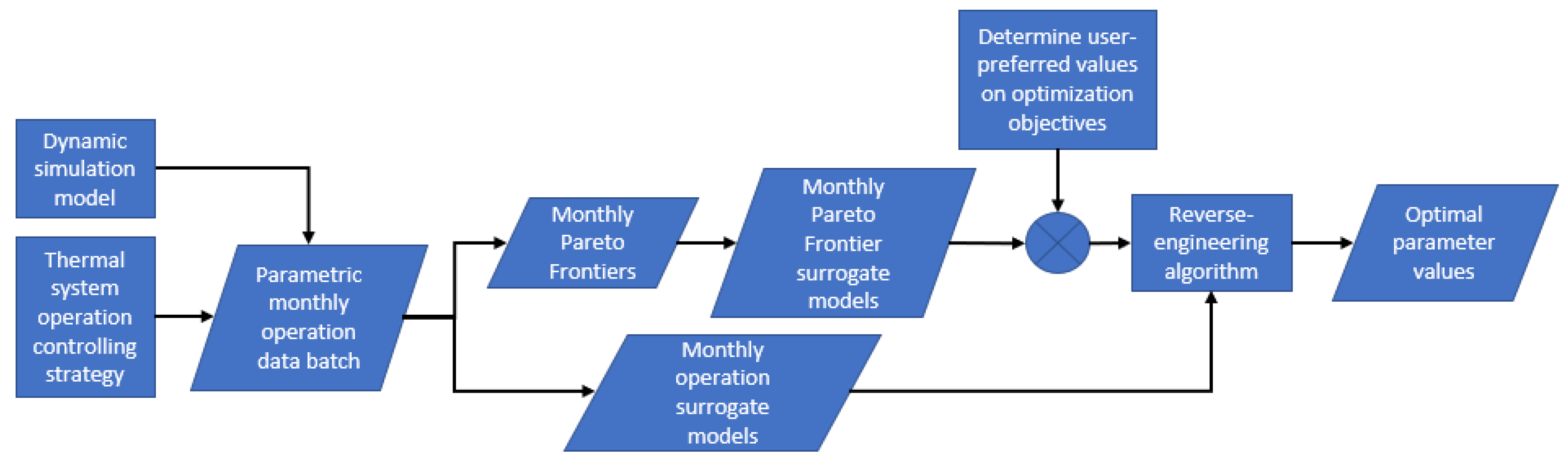
These elements were used in conjunction with each other. More specifically, the thermal system simulation model was first set up, along with the controlling strategies that were adopted during its operation. Parametric monthly operation simulations provided data batches necessary for the construction of monthly operation surrogate models with the use of the surrogate model software.
After data batch generation, the following steps took place:
- Generation of the monthly Pareto frontiers
Monthly Pareto frontiers [30] were developed, i.e., a depiction of the multiobjective optimization solutions in terms of the specified optimization objectives.
- Generation of the monthly Pareto frontier surrogate models and monthly operation surrogate models
Surrogate model of the monthly Pareto frontiers was also formed with the help of the surrogate modeling software as well as the objective data that formed the previously created monthly Pareto frontiers. At the same time, surrogate models of thermal system monthly operation were also created using the surrogate modeling software and the operation data. More specifically, these data were the system parameters and the monthly performance of the systems in terms of the optimization objectives.
- Determination of user-preferred values on optimization objectives
At this time, the methodology had already provided two surrogate model types. The monthly Pareto frontier surrogate models provided each month a correlation between each of the optimization objectives for only the optimal thermal system cases. In other words, by setting a specific objective value, one would be able to know the values of the other optimization objectives that describe an optimal case of the thermal system for each month of the year.
- Determination of the optimal design and operation parameter values through reverse-engineering algorithm
The second surrogate model type, namely, the monthly operation surrogate models essentially provided a correlation between the design as well as the operation parameters of the thermal system and the optimization objectives for every month. If the above two types of surrogate models operate together in combination with a search algorithm, it is possible to determine the design and operation parameters of a thermal system for specified optimization objectives. The reverse-engineering procedure will be elaborated in the next subsection. It should be noted that this layout supports only two optimization objectives, although there is no restriction to what those objectives could be. While available information is based on monthly system operations, it is possible for optimization to take place on an annual basis using the developed indexes that will be elaborated in the next subsection.
The summarized methodology steps can be viewed in Figure 1.
2.2. System Model
For the simulation of the solar-assisted geothermal heat pump, an iterative node-based dynamic model was constructed in Python using physical equations proposed by TRNSYS [31] as well as other sources, as will be elaborated below.
To begin with, the thermal storage tank models developed in Python used the equations based on Type 4: stratified fluid storage tank of TRNSYS [31]. The solar collector model operated according to the following equation (Equation (1)) [31,32]:
where
- no (- ): solar collector optical efficiency;
- Isol (W): solar radiation incident to the collector;
- U (W/m2·K): heat loss factor;
- Qsol (W): heating power produced by the collector by collecting the incident solar radiation Isol (W);
- Tm (°C): average solar collector temperature;
- Tenv (°C): environmental temperature.
The heat pump efficiency model was based on the work of [33]. More specifically, as already stated, the heat pump used was a geothermal heat pump, whose efficiency is described by the following equation (Equation (2)):
where
- COP (-): heat pump efficiency;
- Two (°C): geothermal heat pump outlet pipe fluid temperature;
- Tg (°C): ground temperature.
Finally, the heat exchangers that were situated in the storage tank followed Equation (3) [31,34,35]:
where
- (W): actual heat transfer;
- ε (-): heat exchanger efficiency;
- (kg/s): fluid mass supply;
- Cp (J/(kg·K)): fluid thermal cap;
- (°C): heat exchanger inlet fluid temperature;
- (°C): thermal storage tank node temperature.
As far as climatic data are concerned, hourly external temperature, ground temperature, and solar radiation data corresponding to existing conditions in the city of Kozani, Greece, were employed [36].
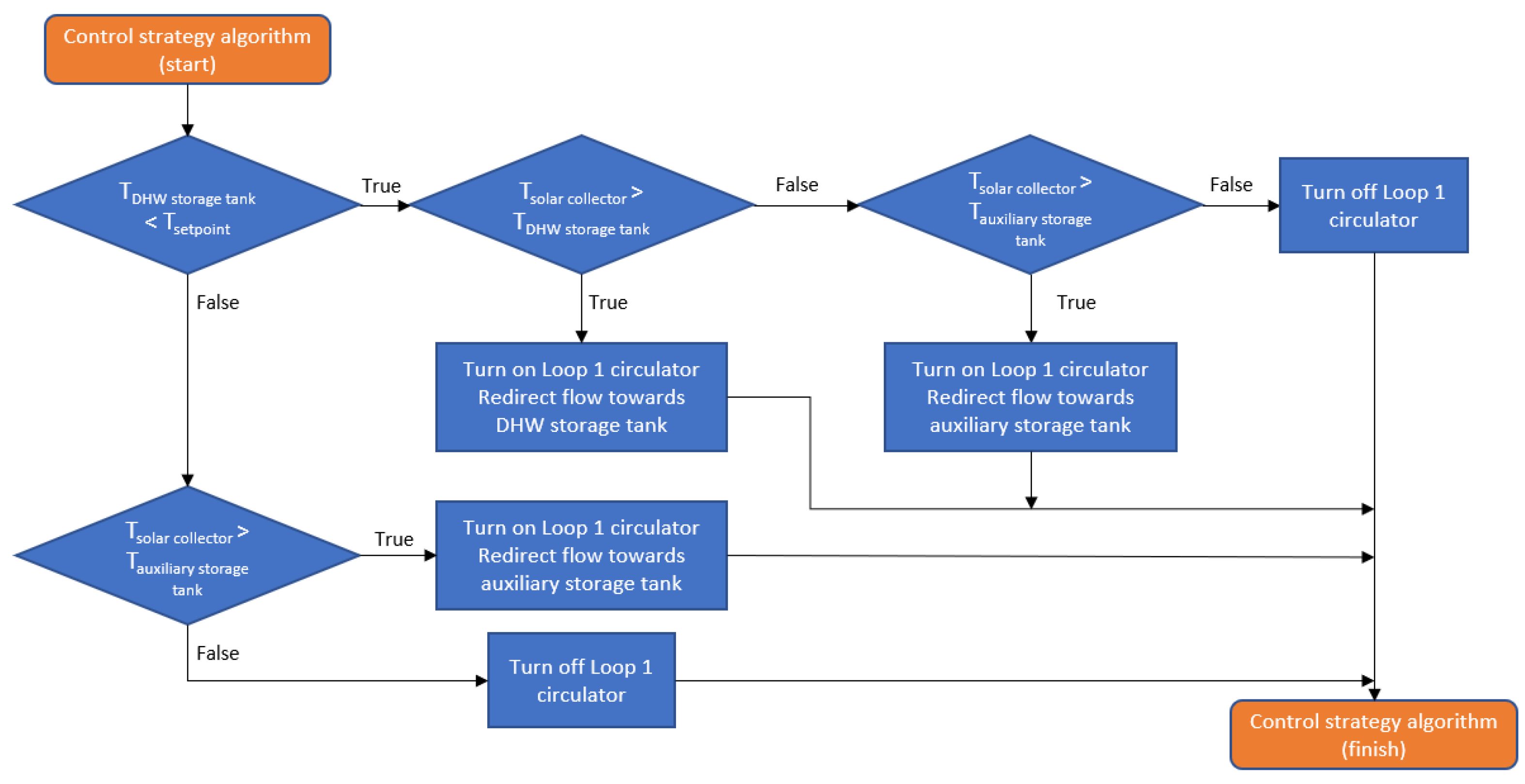
The surrogate model software used for the current case was the ALAMO software [37], which produces simple yet accurate models. Moreover, the controlling strategy adopted in this case was as follows (Figure 2):
- When the solar collector is warmer than the DHW storage tank, the control strategy prioritizes the heating of the DHW storage tank up until the respective setpoint has been attained.
- Any excess solar energy will then be provided to the auxiliary storage tank, provided the solar collector is warmer than the auxiliary tank.
- In case the collector is colder than both tanks, the circulator remains inactive.
Throughout the day, a DHW consumption profile was set. This, along with heat losses, resulted in both tanks getting colder over time. Thus, the solar collector controlling strategy ensures that DHW storage tank temperature levels [32] would be satisfied as much as possible.
2.3. System Parameters
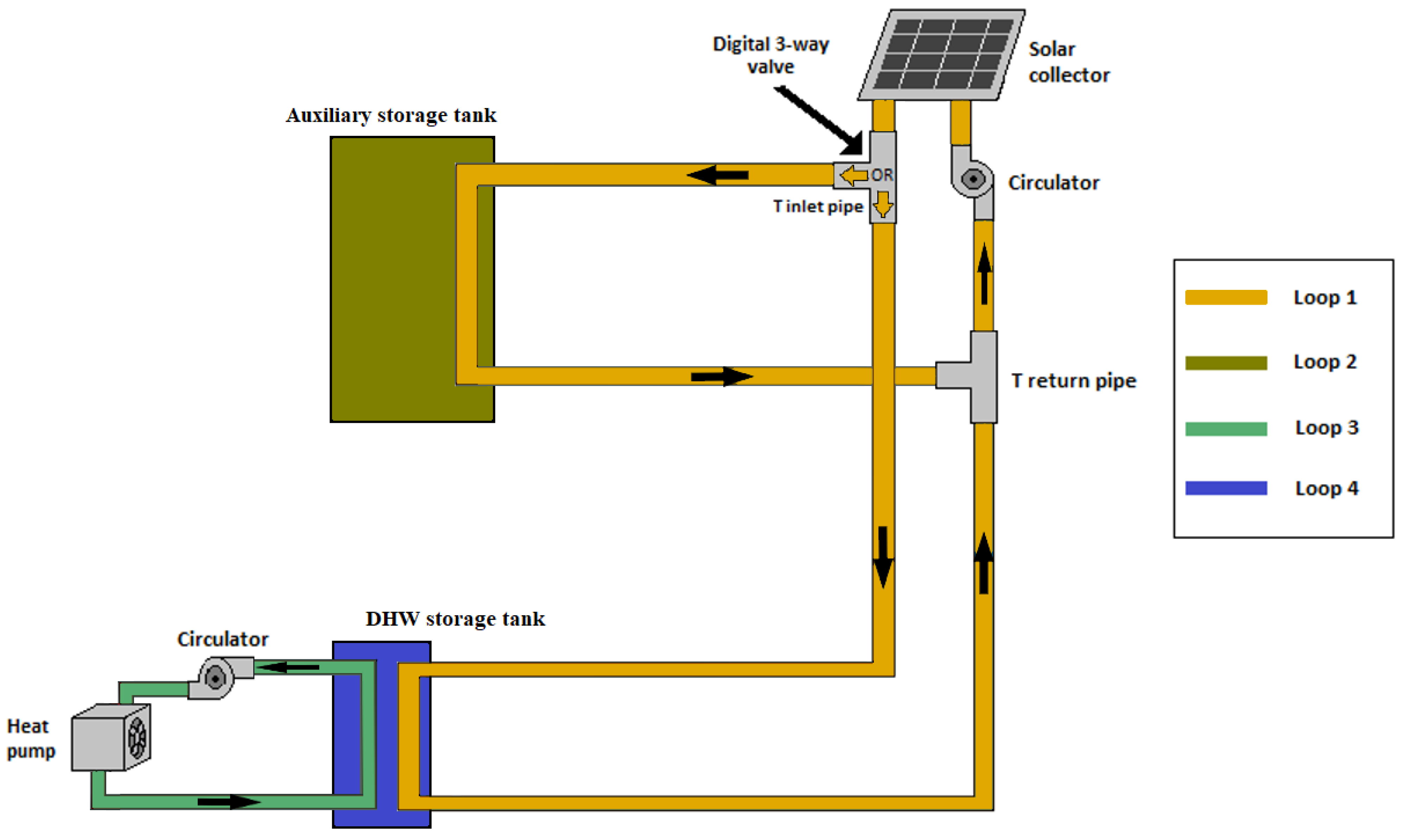
In this subsection of the study, a case example optimization is provided in order for the methodology to be practically demonstrated. The case thermal system presented featured a solar-assisted geothermal heat pump (GHP) setup linked indirectly with two separate thermal storage tanks through their respective heat exchangers. One was responsible for covering the hourly DHW demands when necessary, while the other served as an auxiliary storage tank in which excess thermal load produced by the solar collector was stored. In order for the methodology to be demonstrated in a simple manner, the case system covered the DHW loads of an office building. The DHW demands aggregated to 10 L per person per day when they were provided over the course of the daily schedule. A layout of the thermal system is presented below (Figure 3). The case parameter ranges are shown in Table 1, and the fixed characteristics of the systems are shown in Table 2. The parameter range used for the solar collector was in compliance with [32].
2.4. Optimization Analysis
The presented methodology was applied for the example case. To begin with, for this case, two optimization criteria were set, i.e., monthly thermal energy consumption and DHW thermal load coverage (Equation (4)), which is an index of DHW load satisfaction. Next, a parametric dynamic simulation was performed for all the months of the year. This created a data batch of multiple design and operation parameter scenarios that were used in the following steps.
where
- TDHWe,i: DHW output pipe temperature (°C)
- TDHWe,set: desired DHW output pipe temperature (°C) (set to 50 °C, according to [32]);
- N: size of DHW temperature data batch during a monthly operation.
Next, two system surrogate models were produced that used operation and design parameters of the solar-assisted HP system (Table 1). In turn, they provided the respective monthly energy consumption and DHW thermal load coverage percentage for each parameter scenario. The surrogate model structure is presented using Equation (5). It should be noted that for this case, only linear and logarithmic correlations were used. However, the surrogate model structure is flexible and can therefore be implemented using other layouts.
where
- Y: optimization criterion (i.e., HP energy consumption, QHP, and DHW thermal load coverage, DHWcov);
- xj,i: surrogate model equation parameter coefficients, with j = 1–13;
- i: month index (January to December).
The next step was to create the Pareto frontier using the created data batch. In this case, the Pareto frontier contained the optimization criteria pair values (HP energy consumption and DHW coverage). Essentially, a Pareto frontier of the monthly energy consumption and thermal load coverage was formed, which consisted of the optimal solution scenarios. Information about optimal system performance can be utilized as a way to optimally dimension the existing system. However, in order for the Pareto frontier to be utilized by the optimization methodology, it must be expressed as a mathematical equation that correlates the two optimization criteria between each other. The equation describing the Pareto frontier surrogate model is described in the following equation (Equation (6)):
where
- QHP,op,i: optimal (minimized) value of monthly geothermal heat pump energy consumption (kJ);
- DHWcov,op,i: optimal (maximized) value of monthly DHW load coverage percentage (%);
- i: month index (January to December);
- xj,i: surrogate model equation parameter coefficients, with j = 1–3.
Building a Pareto frontier surrogate model enables the user to demand a criterion to be set at a certain value to obtain the optimal value of the second criterion. For example, if the model user states that their optimal system should cover at least 95% of the DHW load demand on a monthly basis, the Pareto surrogate model returns the minimized (optimal) energy consumption for this case. This procedure is repeated for every month of the year, so the user receives the optimal paired criterion values for an annual operation of the thermal system.
Finally, with information of the optimal performance, the last step was to find the proper dimensioning characteristics of the system whose performance is as close as possible to that of the optimal on an annual basis. As both the Pareto frontier surrogate models and the thermal system performance surrogate models were already available, a reverse-engineering procedure was carried out. In the following subsection, the reverse-engineering procedure is explained.
2.5. Reverse-Engineering Procedure
To begin with, as already explained, the main objective of this procedure is to find the system that operates as close as possible to the optimal on an annual basis, and this means it should operate in that way every month. If the focus is set on a monthly basis, the monthly operation performance of the system can be evaluated using the thermal system surrogate models that are based on Equation (5). Furthermore, the optimal pair of objective values gained from the Pareto frontier surrogate model (Equation (6)) will serve as the target pair of values. All that remains is for the distance between paired criterion values to be measured, produced by the thermal system surrogate models and the optimal paired values from the Pareto frontier surrogate model. The previous sentence can be expressed using Equation (7).
Essentially, monthly performance relative error (MPRE) informs the normalized performance deviation of the thermal system with certain parameter values from the performance of the optimal thermal system scenario. As MPRE had been evaluated, an annual evaluation also had to be performed using the MPRE values of Equation (7). Therefore, the annual performance relative error index (APRE) was calculated using Equation (8).
APRE indicates the root sum of square monthly performance deviations of a chosen thermal system scenario performance from its optimal counterpart on an annual basis. This means the smaller the value, the closer the system is to satisfying the desired optimization criteria on an annual basis. Ultimately, for each set of chosen parameters, by performing the final step of the methodology, an APRE value is extracted. Therefore, using a search algorithm, the optimization procedure finishes at the time a set of thermal system parameters that has the minimum APRE value is found.
3. Results
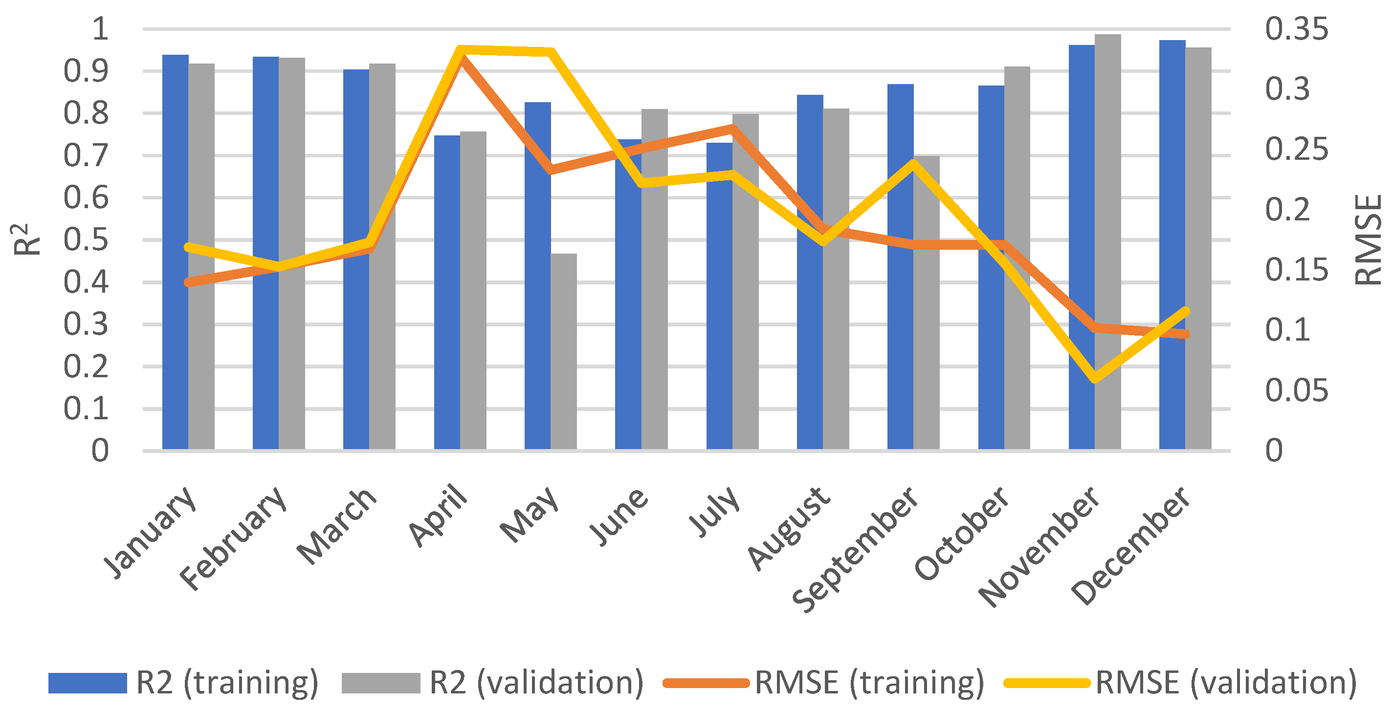
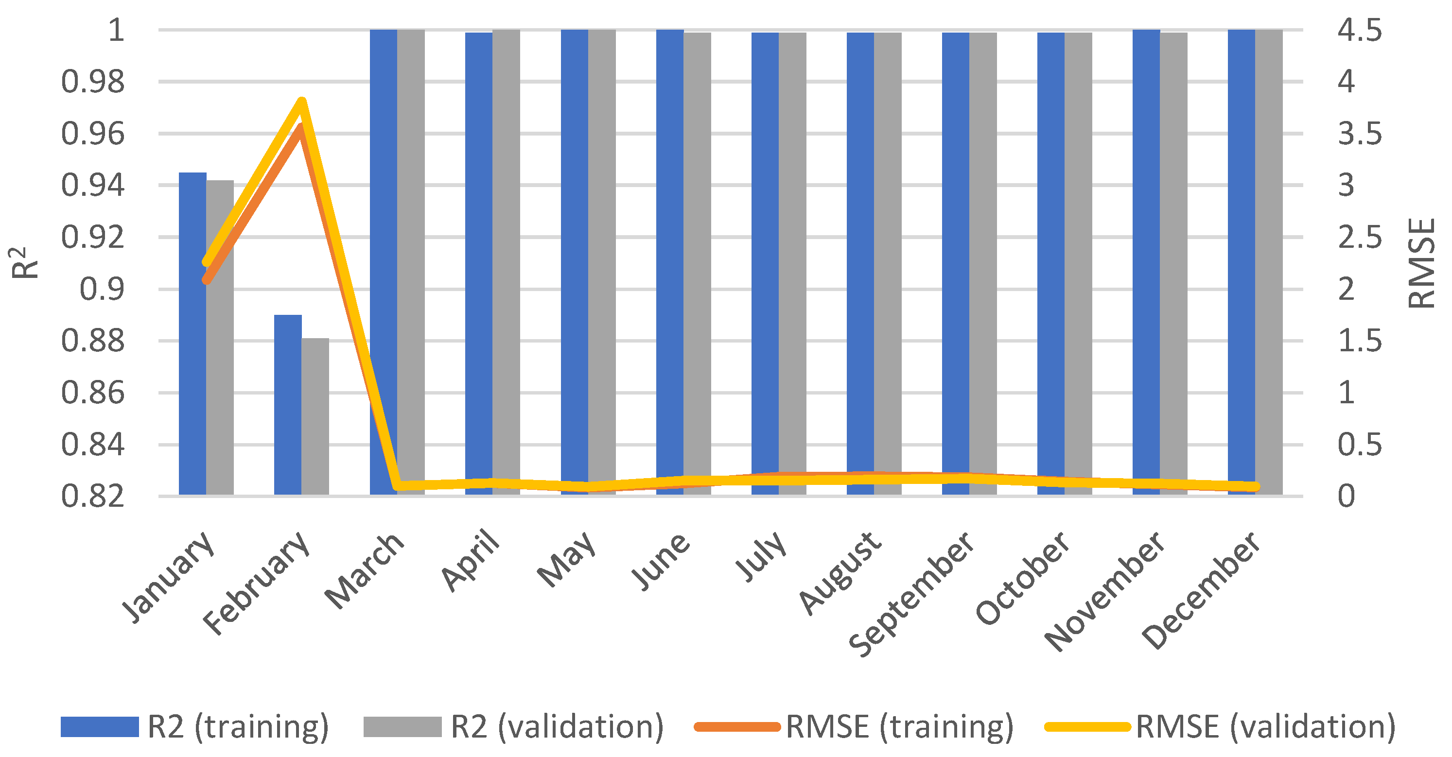
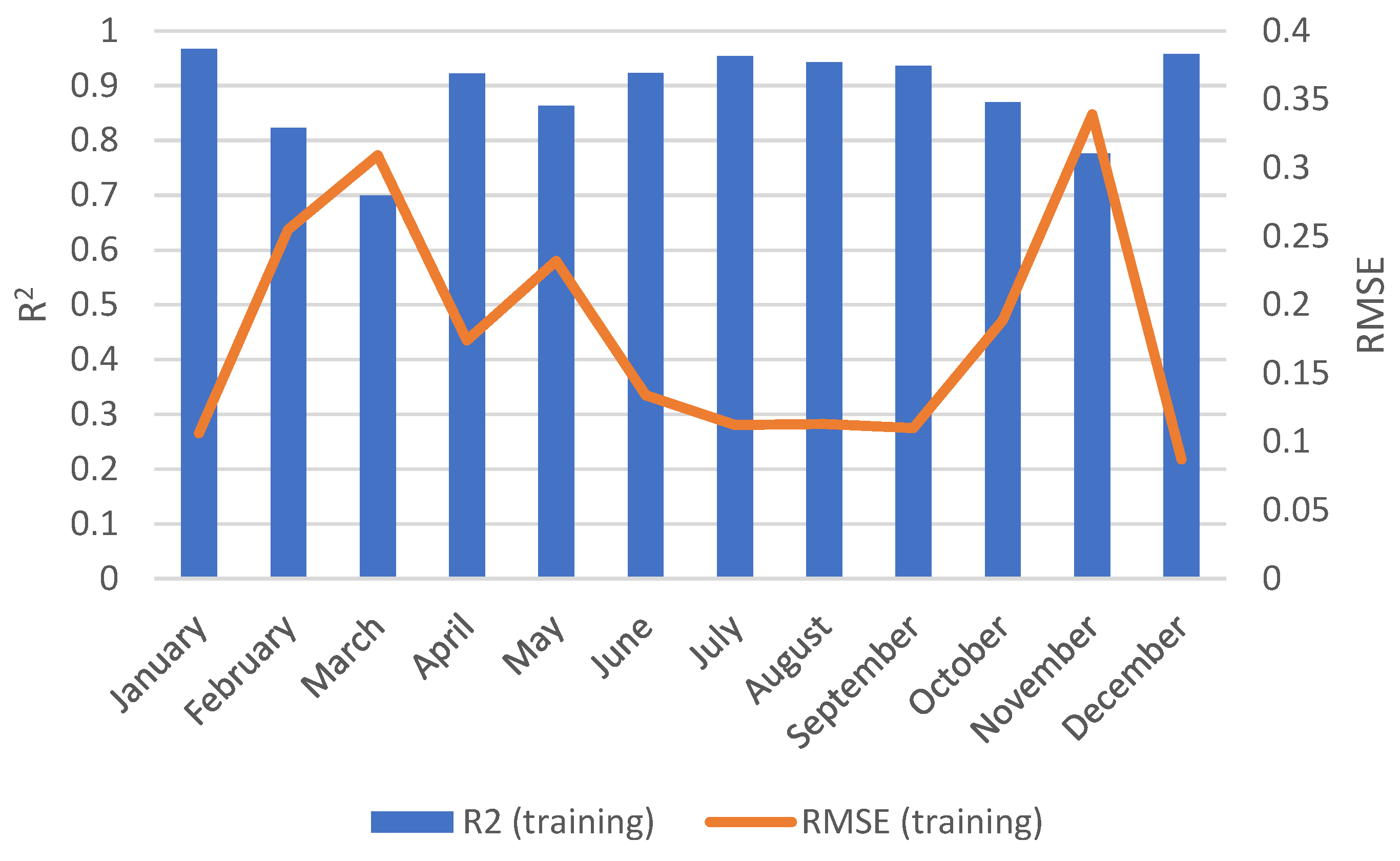
In this section, the case study results from the implementation of the methodology are presented. First of all, the monthly operation surrogate models of the thermal system are exhibited. More specifically, the first surrogate model expresses the correlation between the thermal system monthly energy consumption and optimization parameters. On the other hand, the second surrogate model expresses the correlation between the thermal system monthly DHW load coverage and optimization parameters. Table 3 and Table 4 show the coefficient values of the surrogate models based on Equation (5) for each month of operation. At the same time, the training results of the monthly operation surrogate models of the thermal system are displayed in Figure 4 and Figure 5. It is noted that for the current case, 75–25% training-to-validation data size ratio was employed. It is also worth reminding that the data were derived from the operation simulation of the thermal system. Each surrogate model training–validation process needed a small amount of computational time (about 0.5 s).
It can be discerned from Figure 4 that monthly thermal system consumption surrogate model training had decent performance results. Fitting accuracy appeared to decrease during summer semester. This might mean that seasonal environmental conditions affect fitting accuracy. More specifically, there was a much larger operation result variation among different parametric scenarios of the solar-assisted geothermal heat pump case. In addition, according to Figure 5, the DHW load coverage model appeared to be mostly accurate, with its accuracy declining during a major part of the winter season.
The monthly Pareto frontiers were constructed using the simulation data. At the same time, monthly Pareto frontier surrogate models were generated based on Equation (6). Fitting performance and coefficient values are displayed in Figure 6 and Table 5, respectively. In the case of the Pareto frontier surrogate model, the number of optimal scenarios was too small, so each data batch was used only in the training process and not in the validation process. As can be seen from Table 5, the surrogate model had a great consistency in fitting accuracy due to the monthly data batch size being too small. The batches were small because only about 5% out of the 400 thermal scenarios each month was deemed as optimal according to the Pareto frontier formation methodology. Consequently, the total scenario data batch size for each month should be increased.
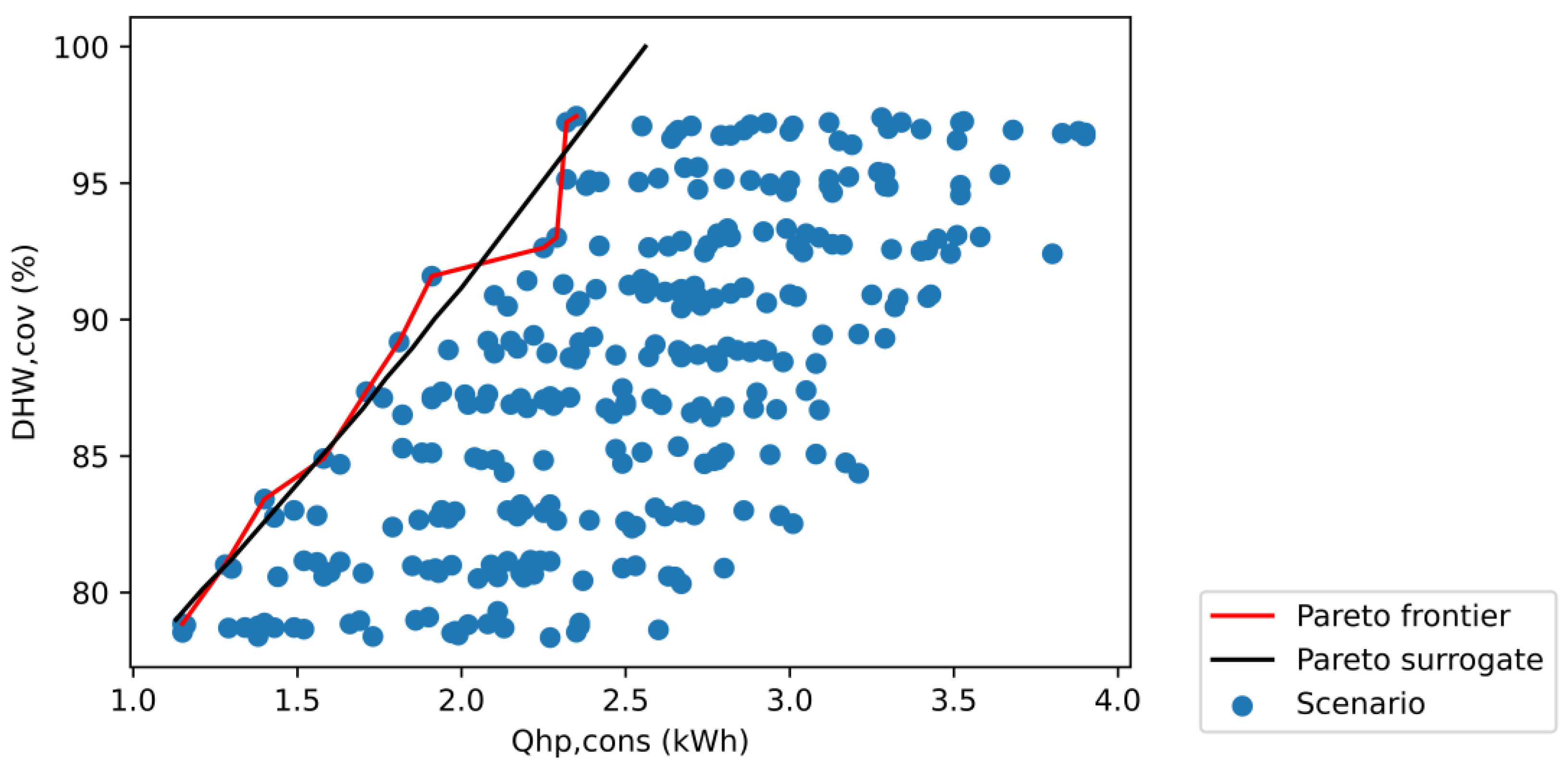
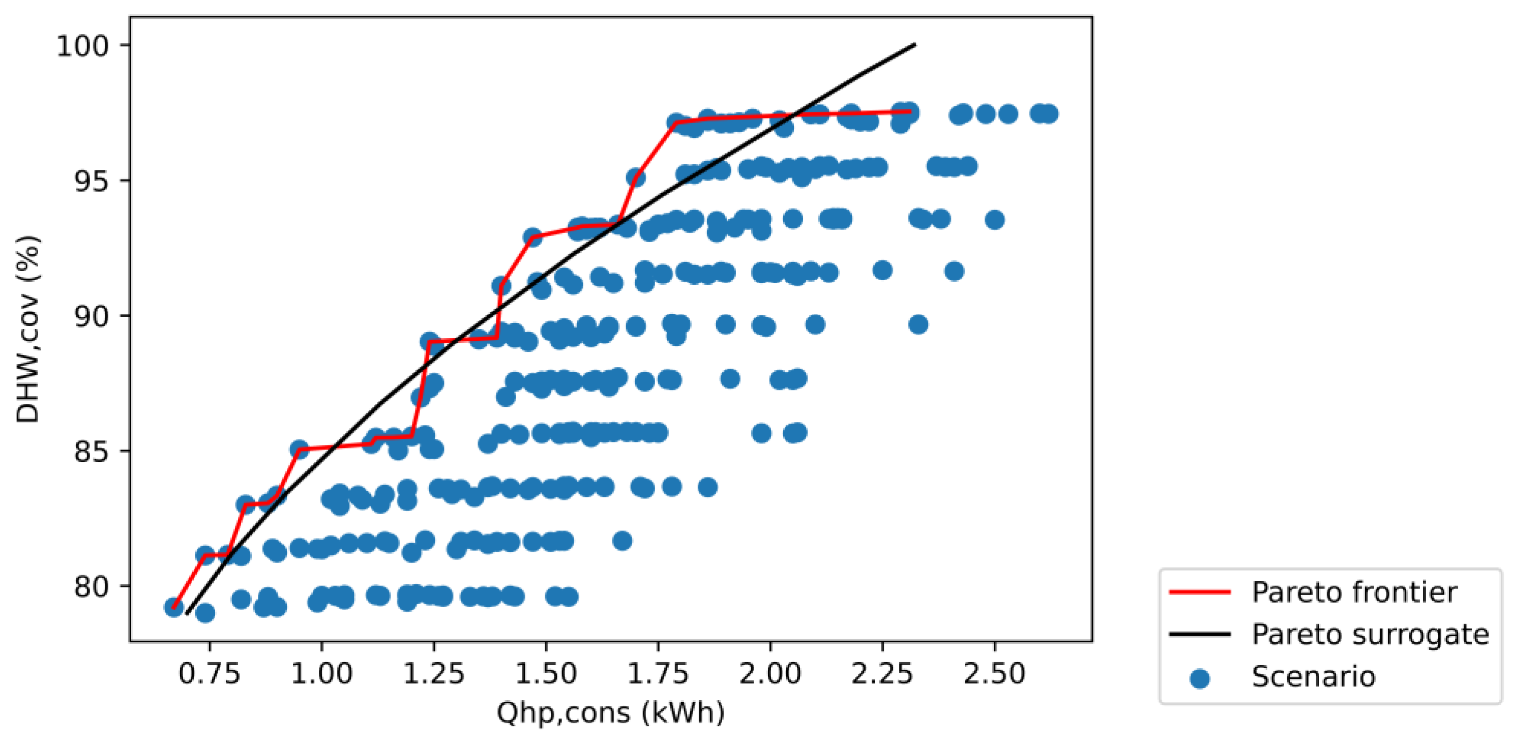
Finally, Figure 7 and Figure 8 exhibit the Pareto frontier along with its respective surrogate model in order to grasp a more practical understanding of the Pareto frontier surrogate models. As can be seen, the solutions forming the Pareto frontier were equally optimal for the optimization objectives (geothermal heat pump energy consumption and domestic hot water coverage). Moreover, they were superior to all the other solutions not belonging to the monthly Pareto frontier. Therefore, these are the solutions that should interest the user during a design process. However, the objective performance of all parameter combinations used are not available to the user, which is why the Pareto frontier surrogate models need to be employed.
Essentially, the Pareto frontier surrogate models allow the user to select a desired objective value for the purpose of optimal thermal system design and then gain the optimal values for the rest of the objectives. For example, if a desired DHW thermal load coverage is set (e.g., 95%), this would allow the determination of the optimum monthly energy consumption. Using the Pareto frontier surrogate models, a monthly energy consumption was extracted for each month, as also observed in Figure 7 and Figure 8. With the optimal pair values for each month (energy consumption and thermal coverage), the reverse-engineering procedure took place. Using a brute force search algorithm in the mentioned parameter value range (Table 1), solutions were provided whose objective values were close to all the monthly optimal paired values and were therefore close to the optimal annual operation for the desired DHW thermal coverage of 95%. These solutions contained various combinations of the optimization parameters that led to an optimally operated system. As an example, 10 runs of the methodology provided solutions that are presented in Table 6, which led to minimized annual energy consumption and 95% DHW annual thermal coverage.
In Table 6, while APRE values at levels of 25% might seem like a substantial error, it corresponds to an average of about 7.2% error for energy consumption and DHW coverage values for each month. Consequently, the methodology is able to provide dimensioning parameter solutions for achieving optimized thermal system performance within an acceptable error margin. However, this error represents how close the system is to the optimal case, which depends on the Pareto frontier surrogate model performance. In addition, APRE is independent from thermal system surrogate models, which means that optimal operation of those parameters is not guaranteed unless thermal system monthly operation surrogate models are accurate enough. In any case, further refining the surrogate model structure accuracy in the future is desirable in order to operate in real cases. This is because retrofitting solutions contain not only the APRE but also the training–validation phase error of the surrogate models.
Moreover, as can be seen from Table 6, multiple runs provide various parameter solutions. Parameter variation for the same objective indicates that there is potential for further constraints to be added. In addition, there is an extensive parameter search range, and some values in that range might not be applicable in real cases. Therefore, the implementation of standardized component dimensioning options is encouraged.
As the design and operation parameter optimization analysis in this work was based on MOO of design and operation parameters of an HVAC system at the same time, it can be compared with the works presented in [23,24] as there are similarities with the respective methodologies. To begin with, the surrogate models of this work were each trained in a short time (1 s), verifying their low computational cost, as also stated in [23]. Their limitation is that the produced model can only be used on buildings of a specific city due to data availability issues. However, in the proposed case, where training data were derived from a dynamic multiparametric simulation, real-time operation data should also be used for the training of surrogate models in an equally effective manner, thus reducing the availability limitations. Furthermore, by examining [24], the proposed study differs in that the proposed methodology also employs surrogate models that correlate the objectives with each other for the optimal cases. With this, a user can start optimization from every direction by setting a specific value on a desired objective. This approach enables the exploitation of the flexibility offered by multiobjective optimization. In addition, the use of monthly surrogate models enables optimization to take place not only at an annual level but also at shorter periods, such as seasonal or semestrial. The flexibility potential of the above methodology has not been highlighted in the existing literature.
4. Conclusions
In this work, a dimensioning methodology for thermal energy systems is presented that addresses the relevant literature gaps. These include the lack of a generalized framework for optimizing design and operation parameters at the same time using an MOO approach. In contrast to existing methodologies, the present method provides not only optimal objective sets but also the design and operation parameters leading to the desired performance should the user wish for a specific system performance setup. Finally, the methodology can be implemented on a monthly, seasonal, or annual basis, essentially being a potentially flexible dimensioning optimization tool.
Through multiparametric simulation, the thermal system performance surrogate model and a Pareto frontier surrogate model were produced. A combination of these models in a reverse-engineering procedure results in a generalized multiobjective dimensioning methodology. The benefits of the proposed methodology include utilization of the flexibility potential of MOO, ease of use, low computational requirements, and a broad context of application in real cases. On the other hand, the implementation of the methodology requires available real-time operation data of the respective thermal system case.
The results of an example case verified the accuracy potential of the surrogate models as well as the ability to determine optimal system parameters in accordance with user-defined optimization criteria. More specifically, the surrogate models had R2 values ranging between 0.85 and 0.9, while RMSE values did not exceed 0.4 as far as monthly energy consumption was concerned. With regard to DHW thermal coverage models, the fitting results were almost identical, except for January and February. Finally, the Pareto frontier surrogate models had acceptable accuracy results for most monthly cases, except for a few cases of mediocre fitting performance (R2 = 0.7).
With regard to optimized dimensioning results, all dimensioning recommendations had an APRE value of about 25%, which corresponded to about 7% error for all monthly surrogate models from the monthly Pareto frontier optimal solutions in terms of objective performance. It is of interest to also notice that when choosing the desired objective value for the dimensioning process, various parameter choices were extracted from the methodology. Last but not least, the implementation of the reverse-engineering procedure was characterized by low computational cost.
The limitations of this study include the need for refinement of the reverse-engineering algorithm, with focus on implementing more advanced search algorithms. In addition, low accuracy surrogate models might be produced in some cases due to the implemented surrogate model form. This issue could be solved using different surrogate model structures as well as fine tuning the training methods. Moreover, the solution variation in practical applications might be excessive, so actions should be taken to further constrain the dimensioning options to real, standardized HVAC component dimensioning. For example, certain technical limitations concerning solar collector or storage tank sizes could be taken into account during the implementation of the methodology, essentially providing only standardized dimension values for each system component. This could also further reinforce the credibility of the dimensioning solutions extracted from the presented methodology implementation. Of course, an additional economical optimization among the presented solutions would further narrow down the available solutions to only a few, which are, in general, the most inexpensive dimensioning solutions to employ. The authors of the present work suggest that the next step could be the development of surrogate models using measurements from existing thermal system cases. Lastly, the MOO approach could be further enhanced through the inclusion of additional criteria, such as economic or environmental ones.
Author Contributions
Conceptualization, L.Z. and G.P.; methodology, L.Z., G.P., and N.P.; software, L.Z. and N.P.; validation, L.Z. and A.K.; formal analysis, L.Z. and A.K.; investigation, L.Z. and A.K.; resources, L.Z. and A.K.; data curation, L.Z., A.K., and N.P.; writing—original draft preparation, L.Z. and G.P.; writing—review and editing, G.P. and N.P.; visualization, L.Z.; supervision, G.P.; project administration, G.P.; funding acquisition, G.P. All authors have read and agreed to the published version of the manuscript.
Funding
We acknowledge support of the project “Development of New Innovative Low Carbon Footprint Energy Technologies to Enhance Excellence in the Region of Western Macedonia” (MIS 5047197), which is implemented under the Action “Reinforcement of the Research and Innovation Infrastructure”, funded by the Operational Program “Competitiveness, Entrepreneurship and Innovation” (NSRF 2014–2020) and co-financed by Greece and the European Union (European Regional Development Fund).
Institutional Review Board Statement
Not applicable.
Informed Consent Statement
Not applicable.
Data Availability Statement
Not applicable.
Conflicts of Interest
The authors declare no conflict of interest. The funders had no role in the design of the study; in the collection, analyses, or interpretation of data; in the writing of the manuscript; or in the decision to publish the results.
Abbreviations
| HVAC | heating, ventilation, and air conditioning |
| MOO | multiobjective optimization |
| DHW | domestic hot water |
| HP | heat pump |
| GHP | geothermal heat pump |
| MPRE | monthly performance relative error |
| APRE | annual performance relative error |
References
- Eurostat. Energy Statistics—An Overview. Available online: https://ec.europa.eu/eurostat/statistics-explained/index.php/Energy_statistics_-_an_overview#Primary_energy_production (accessed on 4 November 2022).
- Pérez-Lombard, L.; Ortiz, J.; Pout, C. A review on buildings energy consumption information. Energy Build. 2008, 40, 394–398. [Google Scholar] [CrossRef]
- ANSI/ASHRAE/IES Standard 90.1-2019; Energy Standard for Buildings Except Low-Rise Residential Buildings. American Society of Heating, Refrigerating and Air Conditioning Engineers: Atlanta, GA, USA, 2019.
- ANSI/ASHRAE/IES Standard 90.2-2018; Energy Efficient Design of Low-Rise Residential Buildings. American Society of Heating, Refrigerating and Air Conditioning Engineers: Atlanta, GA, USA, 2018.
- European Parliament and Council of the European Union. Directive (EU) 2018/844 of the European Parliament and of the Council of 30 May 2018 Amending Directive 2010/31/EU on the Energy Performance of Buildings and Directive 2012/27/EU on Energy Efficiency (Text with EEA Relevance). Available online: https://eur-lex.europa.eu/eli/dir/2018/844/oj (accessed on 4 November 2022).
- Magni, M.; Ochs, F.; de Vries, S.; Maccarini, A.; Sigg, F. Detailed cross comparison of building energy simulation tools results using a reference office building as a case study. Energy Build. 2021, 250, 111260. [Google Scholar] [CrossRef]
- Guelpa, E.; Verda, V. Compact physical model for simulation of thermal networks. Energy 2019, 175, 998–1008. [Google Scholar] [CrossRef]
- Gambarotta, A.; Morini, M.; Rossi, M.; Stonfer, M. A Library for the Simulation of Smart Energy Systems: The Case of the Campus of the University of Parma. Energy Procedia 2017, 105, 1776–1781. [Google Scholar] [CrossRef]
- Queipo, N.V.; Haftka, R.T.; Shyy, W.; Goel, T.; Vaidyanathan, R.; Tucker, P.K. Surrogate-based analysis and optimization. Prog. Aerosp. Sci. 2005, 41, 1–28. [Google Scholar] [CrossRef] [Green Version]
- Blum, D.; Wang, Z.; Weyandt, C.; Kim, D.; Wetter, M.; Hong, T.; Piette, M.A. Field demonstration and implementation analysis of model predictive control in an office HVAC system. Appl. Energy 2022, 318, 119104. [Google Scholar] [CrossRef]
- Biemann, M.; Scheller, F.; Liu, X.; Huang, L. Experimental evaluation of model-free reinforcement learning algorithms for continuous HVAC control. Appl. Energy 2021, 298, 117164. [Google Scholar] [CrossRef]
- Jiang, Z.; Risbeck, M.J.; Ramamurti, V.; Murugesan, S.; Amores, J.; Zhang, C.; Lee, Y.M.; Drees, K.H. Building HVAC control with reinforcement learning for reduction of energy cost and demand charge. Energy Build. 2021, 239, 110833. [Google Scholar] [CrossRef]
- Gonçalves, D.; Sheikhnejad, Y.; Oliveira, M.; Martins, N. One step forward toward smart city Utopia: Smart building energy management based on adaptive surrogate modelling. Energy Build. 2020, 223, 110146. [Google Scholar] [CrossRef]
- Wang, H.; Wang, S. A hierarchical optimal control strategy for continuous demand response of building HVAC systems to provide frequency regulation service to smart power grids. Energy 2021, 230, 120741. [Google Scholar] [CrossRef]
- Sha, H.; Xu, P.; Hu, C.; Li, Z.; Chen, Y.; Chen, Z. A simplified HVAC energy prediction method based on degree-day. Sustain. Cities Soc. 2019, 51. [Google Scholar] [CrossRef]
- Stanica, D.-I.; Karasu, A.; Brandt, D.; Kriegel, M.; Brandt, S.; Steffan, C. A methodology to support the decision-making process for energy retrofitting at district scale. Energy Build. 2021, 238, 110842. [Google Scholar] [CrossRef]
- Allen, A.; Henze, G.; Baker, K.; Pavlak, G.; Murphy, M. An optimization framework for the network design of advanced district thermal energy systems. Energy Convers. Manag. 2022, 266. [Google Scholar] [CrossRef]
- Lantonio, N.A.; Krarti, M. Simultaneous design and control optimization of smart glazed windows. Appl. Energy 2022, 328. [Google Scholar] [CrossRef]
- Clarke, F.; Dorneanu, B.; Mechleri, E.; Arellano-Garcia, H. Optimal design of heating and cooling pipeline networks for residential distributed energy resource systems. Energy 2021, 235, 121430. [Google Scholar] [CrossRef]
- Knudsen, B.R.; Rohde, D.; Kauko, H. Thermal energy storage sizing for industrial waste-heat utilization in district heating: A model predictive control approach. Energy 2021, 234, 121200. [Google Scholar] [CrossRef]
- Rohde, D.; Knudsen, B.R.; Andresen, T.; Nord, N. Dynamic optimization of control setpoints for an integrated heating and cooling system with thermal energy storages. Energy 2019, 193, 116771. [Google Scholar] [CrossRef]
- Chang, K.-H. Multiobjective Optimization and Advanced Topics. Des. Theory Methods Using CAD/CAE 2015, 4, 325–406. [Google Scholar] [CrossRef]
- Thrampoulidis, E.; Mavromatidis, G.; Lucchi, A.; Orehounig, K. A machine learning-based surrogate model to approximate optimal building retrofit solutions. Appl. Energy 2020, 281, 116024. [Google Scholar] [CrossRef]
- Starke, A.R.; Cardemil, J.M.; Colle, S. Multi-objective optimization of a solar-assisted heat pump for swimming pool heating using genetic algorithm. Appl. Therm. Eng. 2018, 142, 118–126. [Google Scholar] [CrossRef]
- Dorotić, H.; Pukšec, T.; Duić, N. Multi-objective optimization of district heating and cooling systems for a one-year time horizon. Energy 2018, 169, 319–328. [Google Scholar] [CrossRef]
- He, Z.; Farooq, A.S.; Guo, W.; Zhang, P. Optimization of the solar space heating system with thermal energy storage using data-driven approach. Renew. Energy 2022, 190, 764–776. [Google Scholar] [CrossRef]
- García-Fuentes, M.; García-Pajares, R.; Sanz, C.; Meiss, A. Novel Design Support Methodology Based on a Multi-Criteria Decision Analysis Approach for Energy Efficient District Retrofitting Projects. Energies 2018, 11, 2368. [Google Scholar] [CrossRef] [Green Version]
- Dirutigliano, D.; Delmastro, C.; Moghadam, S.T. Energy efficient urban districts: A multi-criteria application for selecting retrofit actions. Int. J. Heat Technol. 2017, 35, S49–S57. [Google Scholar] [CrossRef]
- Bagheri-Esfeh, H.; Dehghan, M.R. Multi-objective optimization of setpoint temperature of thermostats in residential buildings. Energy Build. 2022, 261, 111955. [Google Scholar] [CrossRef]
- Goodarzi, E.; Ziaei, M.; Hosseinipour, E.Z. Introduction to Optimization Analysis in Hydrosystem Engineering; Springer International Publishing: New York, NY, USA, 2014. [Google Scholar] [CrossRef]
- Klein S., A.; Beckman, W.A. TRNSYS 16: A transient system simulation program: Mathematical reference. TRNSYS 2007, 5, 389–396. [Google Scholar]
- Duffie, J.A.; Beckman, W.A.; Blair, N. Solar Engineering of Thermal Processes, Photovoltaics and Wind, 5th ed.; Wiley: Hoboken, NJ, USA, 2020. [Google Scholar]
- Mouzeviris, G.A.; Papakostas, K.T. Comparative analysis of air-to-water and ground source heat pumps performances. Int. J. Sustain. Energy 2020, 40, 69–84. [Google Scholar] [CrossRef]
- Kays, W.M.; London, A.L. Compact Heat Exchangers; Krieger Publishing Company: Malabar, FL, USA, 1998. [Google Scholar]
- Bergman, T.L.; Lavine, A.S.; Incropera, F.P.; DeWitt, D.P. Introduction to Heat Transfer, 6th ed.; Wiley: Hoboken, NJ, USA, 2011. [Google Scholar]
- TEE. Greek Technical Chamber, Technical Directive 20701-3: Climatic Data for Greek Areas; TEE: Athens, Greece, 2010. [Google Scholar]
- Cozad, A.; Sahinidis, N.V.; Miller, D.C. A combined first-principles and data-driven approach to model building. Comput. Chem. Eng. 2015, 73, 116–127. [Google Scholar] [CrossRef]
Figure 1.
Layout of the proposed multiobjective design and operation dimensioning methodology.

Figure 2.
Solar-assisted geothermal heat pump control strategy flow chart.

Figure 3.
Solar-assisted geothermal heat pump layout.

Figure 4.
Monthly thermal system energy consumption (QHP) model training and validation performance.
Figure 4.
Monthly thermal system energy consumption (QHP) model training and validation performance.

Figure 5.
Monthly DHW thermal coverage (DHWcov) surrogate model training and validation performance.
Figure 5.
Monthly DHW thermal coverage (DHWcov) surrogate model training and validation performance.

Figure 6.
Monthly Pareto frontier surrogate model training performance.

Figure 7.
Pareto frontier of the system monthly operation during December.

Figure 8.
Pareto frontier of the system monthly operation during August.


Table 1.
Parameter value ranges.
| Symbol | Description | Value Range | Unit | ||
|---|---|---|---|---|---|
| H | DHW storage tank height (m) | 0.18–0.55 0.1–0.5 40–50 | m | ||
| mHP | HP water mass supply (kg/s) | kg/s | |||
| THP,set | HP heating temperature setpoint (°C) | °C | |||
| no | Solar collector optical efficiency | 0.82 | 0.75 | 0.57 | - |
| Ul | Solar collector heat loss factor | 7.5 | 5 | 1.82 | W·m−2·K−1 |
| Asol | Solar collector area (m2) | 2–7 | m2 | ||
Table 2.
Fixed characteristics of the case system.
| Description | Value | Unit |
|---|---|---|
| Auxiliary storage tank height | 1 | m |
| Auxiliary storage tank radius | 0.4 | m |
| Auxiliary storage tank volume | 500 | lt |
| Auxiliary storage tank heat loss factor | 0.07 | W·m−2·K−1 |
| Auxiliary storage tank set point | 60 | °C |
| DHW storage tank radius | 0.3 | m |
| DHW storage tank set point | 40 | °C |
| Heat exchangers effectiveness | 0.85 | - |
| Geothermal Heat pump circulator power | 1000 | W |
| Solar collector operational mass supply | 0.1 | kg/s |
Table 3.
Thermal system energy consumption (QHP) surrogate model coefficients produced from model training.
Table 3.
Thermal system energy consumption (QHP) surrogate model coefficients produced from model training.
| Month | Χ1 | Χ2 | Χ3 | Χ4 | Χ5 | Χ6 | Χ7 | Χ8 | Χ9 | Χ10 | Χ11 | Χ12 | X13 |
|---|---|---|---|---|---|---|---|---|---|---|---|---|---|
| January | 2.88 | −0.19 | 0.12 | 0 | 0 | −1.71 | 0 | 0.94 | 0 | −0.48 | 7.74 | 0 | 0 |
| February | 0 | 0 | 0.47 | 0 | 0 | 0 | 2.86 | 0.30 | −15.91 | −0.51 | 1.35 | 0 | 39.93 |
| March | 0 | 0 | 0.13 | 0 | −5.29 | 0 | 1.15 | 0 | 0 | −0.52 | 0 | 0.85 | 0 |
| April | 1.88 | 0 | 0.14 | 0 | −8.93 | 0.31 | 0 | 0 | 0 | −0.44 | 0 | 0 | 0 |
| May | 2.78 | 0 | 0.12 | 0 | 0 | 0 | 0 | 0 | 0 | −0.40 | 6.42 | −1.68 | 0 |
| June | 5.71 | 0 | 0.12 | 0 | 0 | 0 | −1.39 | 0 | 0 | −0.35 | 10.55 | −2.72 | 0 |
| July | 1.40 | 0 | 0.14 | 0 | −5.47 | 0 | 0 | 0 | 0 | −0.29 | 4.24 | 0 | 0 |
| August | 1.71 | 0 | 0.12 | 0 | 0 | 0 | 0 | 0 | 0 | −0.31 | 6.75 | −1.71 | 0 |
| September | 2.06 | 0 | 0.15 | 0 | 0 | 0 | 0 | 0 | −1.57 | −0.35 | 0 | −0.65 | 0 |
| October | 2.35 | 0 | 0.12 | 0 | 0 | 0 | 0 | 0 | 0 | −0.36 | 6.20 | −1.58 | 0 |
| November | 3.13 | 0 | 0.16 | 0 | 0 | 0 | 0 | 0 | −1.78 | −0.43 | 0 | 0 | 0 |
| December | 3.54 | 0 | 0.41 | 0 | 0 | 0 | 0 | 0 | −12.40 | −0.49 | −0.13 | 0 | 29.40 |
Table 4.
DHW thermal coverage (DHWcov) surrogate model coefficients produced from model training.
| Month | Χ1 | Χ2 | Χ3 | Χ4 | Χ5 | Χ6 | Χ7 | Χ8 | Χ9 | Χ10 | Χ11 | Χ12 | X13 |
|---|---|---|---|---|---|---|---|---|---|---|---|---|---|
| January | 19.23 | −1.92 | 1.62 | −3.15 | 0 | −1.09 | −10.35 | 14.67 | 0 | 0 | 58.12 | 0 | 0 |
| February | −20.18 | 1.94 | 0 | 0 | 0 | 0 | 0 | 12.57 | 0 | 0 | 49.07 | 0 | 0 |
| March | 1.78 | 0.09 | 2.32 | 0 | 0 | 0.06 | −0.37 | −0.48 | −14.05 | 0 | 0 | 0 | 37.60 |
| April | 2.25 | 0 | 2.33 | 0 | 0 | 0.05 | 0 | −0.18 | −15.50 | 0 | 0 | 0 | 42.38 |
| May | −1.80 | 0.07 | 2.23 | 0 | −6.80 | 0 | 1.54 | −0.39 | −12.31 | 0 | −4.35 | 0 | 31.67 |
| June | −6.15 | 0 | 1.90 | 0 | 0 | 0 | 3.00 | −0.15 | −2.55 | 0 | 0 | 0 | 0 |
| July | −4.96 | 0 | 1.45 | 0 | 0 | 0 | 2.37 | −0.14 | 23.64 | 0 | 0 | 0 | −61.31 |
| August | −4.49 | 0 | 1.56 | 0 | 0 | 0 | 2.10 | 0 | 18.37 | 0 | 0 | 0 | −46.89 |
| September | −4.45 | 0 | 1.91 | 0 | 0 | 0 | 2.45 | −0.08 | 2.00 | 0 | 0 | 0 | 0 |
| October | 0 | 0.12 | 1.96 | 0 | 2.71 | 0 | 0.85 | −0.62 | 0 | 0 | −1.60 | 0 | 0 |
| November | 2.74 | 0 | 2.03 | 0 | 1.58 | 0 | −0.70 | −0.08 | −1.21 | 0 | 0 | 0 | 0 |
| December | 0 | 0 | 2.02 | 0 | 0 | 0 | −0.10 | −0.08 | 0 | 0 | 0 | 0.25 | −1.43 |
Table 5.
Monthly Pareto frontier surrogate model coefficients produced from model training.
| Month | Χ1 | Χ2 | Χ3 |
|---|---|---|---|
| January | 0.45 | −30.00 | 97.33 |
| February | 0.34 | −24.16 | 79.96 |
| March | 0.11 | −1.70 | 0 |
| April | 0 | 7.69 | −32.46 |
| May | 0.73 | −57.46 | 194.55 |
| June | 0.51 | −38.34 | 128.49 |
| July | 0.10 | −1.72 | 0 |
| August | 0.36 | −25.30 | 82.83 |
| September | 0.41 | −30.02 | 99.91 |
| October | 0.73 | −57.81 | 196.15 |
| November | 1.42 | −118.03 | 405.05 |
| 12 | 0 | 6.06 | −25.03 |
Table 6.
Multiobjective optimization dimensioning results for 10 runs of the reverse-engineering procedure (desired DHW thermal coverage at 95%).
Table 6.
Multiobjective optimization dimensioning results for 10 runs of the reverse-engineering procedure (desired DHW thermal coverage at 95%).
| Solution No. | DHW Storage Tank Height (m) | HP Water Mass Supply (kg/s) | HP Heating Temperature Setpoint (°C) | Solar Collector Maximum Efficiency (-) | Solar Collector Heat Loss Factor (W·m−2·K−1) | Solar Collector Area (m2) | APRE |
|---|---|---|---|---|---|---|---|
| 1 | 0.35 | 0.36 | 42 | 0.57 | 1.82 | 4.1 | 0.246 |
| 2 | 0.52 | 0.24 | 43 | 0.57 | 1.82 | 6.8 | 0.252 |
| 3 | 0.36 | 0.13 | 49 | 0.75 | 5 | 5.5 | 0.249 |
| 4 | 0.18 | 0.36 | 42 | 0.75 | 5 | 5.4 | 0.249 |
| 5 | 0.35 | 0.26 | 41 | 0.57 | 1.82 | 2.2 | 0.247 |
| 6 | 0.36 | 0.46 | 40 | 0.75 | 5 | 5.7 | 0.249 |
| 7 | 0.36 | 0.20 | 40 | 0.75 | 5 | 5.2 | 0.251 |
| 8 | 0.53 | 0.49 | 48 | 0.75 | 5 | 2.5 | 0.249 |
| 9 | 0.35 | 0.24 | 40 | 0.82 | 7.50 | 5.6 | 0.249 |
| 10 | 0.34 | 0.33 | 47 | 0.57 | 1.82 | 6.3 | 0.248 |
Disclaimer/Publisher’s Note: The statements, opinions and data contained in all publications are solely those of the individual author(s) and contributor(s) and not of MDPI and/or the editor(s). MDPI and/or the editor(s) disclaim responsibility for any injury to people or property resulting from any ideas, methods, instructions or products referred to in the content. |
© 2023 by the authors. Licensee MDPI, Basel, Switzerland. This article is an open access article distributed under the terms and conditions of the Creative Commons Attribution (CC BY) license (https://creativecommons.org/licenses/by/4.0/).
Share and Cite
MDPI and ACS Style
Zouloumis, L.; Karanasos, A.; Ploskas, N.; Panaras, G. Multicriteria Design and Operation Optimization of a Solar-Assisted Geothermal Heat Pump System. Energies 2023, 16, 1266. https://0-doi-org.brum.beds.ac.uk/10.3390/en16031266
AMA Style
Zouloumis L, Karanasos A, Ploskas N, Panaras G. Multicriteria Design and Operation Optimization of a Solar-Assisted Geothermal Heat Pump System. Energies. 2023; 16(3):1266. https://0-doi-org.brum.beds.ac.uk/10.3390/en16031266
Chicago/Turabian StyleZouloumis, Leonidas, Angelos Karanasos, Nikolaos Ploskas, and Giorgos Panaras. 2023. "Multicriteria Design and Operation Optimization of a Solar-Assisted Geothermal Heat Pump System" Energies 16, no. 3: 1266. https://0-doi-org.brum.beds.ac.uk/10.3390/en16031266
Note that from the first issue of 2016, this journal uses article numbers instead of page numbers. See further details here.