On the Exact Analytical Formulas of Leakage Current-Based Supercapacitor Model Operating in Industrial Applications

Abstract

The resistance–capacitance (RC) model is one of the most applicable circuits for modeling the charging and discharging processes of supercapacitors (SCs). Although this circuit is usually used in the electric and thermal investigation of the performance of SCs, it does not include leakage currents. This paper presents exact analytical formulas of leakage-current-based supercapacitor models that can be used in industrial applications, i.e., constant-power-based applications. In the proposed model, current and voltage are represented as a solution of nonlinear equations that are solved using the standard Newton method. The proposed expressions’ accuracy is compared with the results obtained using traditional numerical integration methods with leakage current formulation and other methods, found in the literature, with no leakage current formulation. The results confirm that including leakage current represents a more accurate and realistic manner of modeling SCs. The results show that the derived expressions are precise, allowing the generation of results that closely match those obtained using traditional numerical-based methods. The derived expressions can be used to investigate SCs further and achieve more accurate and efficient regulation and control of SCs in different applications.

1. Introduction

Modern electricity systems cannot function without energy storage systems (ESSs). Furthermore, without ESSs, managing future power systems efficiently and profitably is challenging [1]. Utilizing ESSs also improves voltage conditions, reduces system losses, increases transmission line capacity, and has other similar effects [2]. In addition, ESSs are vital for power networks with a high penetration of renewable energy sources, since they help to smooth out the intermittent character of these sources [3]. In transportation, ESSs are also commonly employed in the auto industry, namely with electric vehicles. The value of ESSs is steadily increasing as electric vehicles become more prevalent [4,5].

There are numerous kinds of ESSs in general [6]. Mechanical systems are the oldest and, at the same time, most powerful systems. These include reversible power plant systems that employ water pools and in which the electric machine can function as both a generator (when power is delivered to the grid) and a motor to start the pump (when water is transferred from a lower-altitude basin to a higher-altitude basin) [7]. Compressed air systems are also included in this category [8]. The foregoing systems, however, share the common property of being territorially dependent. Aside from them, specific systems rely on chemical reactions to function. The most prominent of this group is batteries [9], which have numerous applications, particularly in electric vehicles [10]. The third category contains systems whose operation is governed by electrical engineering principles. This category includes supercapacitors (SCs) [11,12,13,14] and super magnetics (SMs) [15]. These storage systems are distinguished by high efficiency, outstanding response speed, low self-discharge currents, and the ability to be integrated into any portion of the power system. These are the primary reasons SMs and SCs are treated more frequently in published research. Moreover, for automotive applications and fuel cells, SCs may deliver a significant amount of power with a quick dynamic response [16].

Regarding SCs, the existing research contains a variety of modeling methodologies. Zhang et al. offered in [13] an overview of their models while focusing on the potential aspects of SC device modeling. Zhang et al. discussed the implementation of SCs from management and control standpoints, described electrical, thermal, and self-discharge processes in SCs, and mentioned other electrochemical, equivalent, intelligent, and fractional-order models. In addition, they highlighted the applications of SC devices. Unlike Zhang’s findings, Mussolini presented in [12] a full-frequency-range model capable of representing all SC-related events. In addition, the research proposed a method for determining the model parameters that can be utilized to characterize the SC before its application.

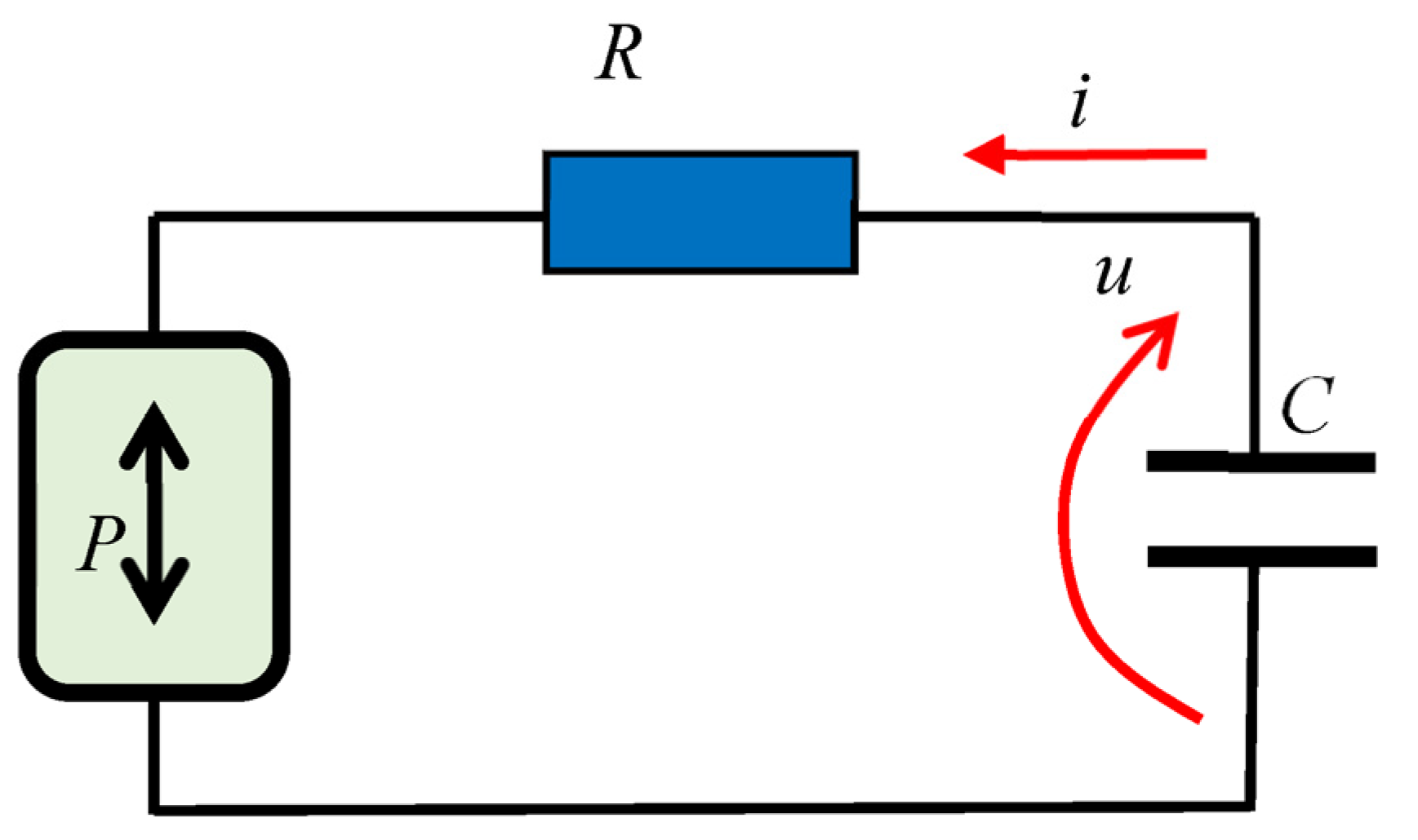
In contrast to the studies of Mussolini and Zhang, Grbovic [17] described SC devices using variable capacitance. The core concern of Grbovic’s work [17] was the analysis, modeling, and design of ultracapacitor modules and their interface with DC–DC power converters. In addition to highlighting the impacts of temperature on the model parameters, comprehensive and approximative models of replacement circuits were offered. In addition, the operating processes in the discharge and charging modes were discussed, along with the design challenge, the connection with converters, and specific application areas. These studies showed that the classic SC model, the resistance–capacitance (RC) model, which consists of capacitance and in-line resistance, can effectively represent the SC charging and discharging process [18,19,20].

The loss term that characterizes internal heating in the capacitor is resistance. The chief benefit of RC models is that their parameters are constant over the entire operating temperature range. It should be noted that the authors in [21] showed that increasing the temperature impacts resistance reduction and increases the capacitance of SC devices.

As explored in [22], due to the vast number of applications for SCs, it is essential to fully understand and accurately evaluate their electric performance in various conditions for accurate assessment and monitoring of their state, control/management when integrated into systems, and their aging prediction. The operation of SC devices at constant current, impedance, and power is presented in [22]. Mathematically, in the constant resistance discharge mode, the instantaneous power provided to the load is expressed using the gamma function in analytical form. In addition, the discharge voltage for a constant discharge current (I_cc) is expressed using the gamma function. In constant power applications, however, the voltage was represented as a differential equation for which the authors provided a numerical predictor–corrector-based solution. The way these devices work electrically depends on several things, such as the chemistry and structure of the materials they are made of, how they store energy, how they are used (such as temperature, type, mode, and rate of charging/discharging waveforms), and how these different things interact with each other [22].

One of the most common ways to use these SCs in real life is in a mode called “constant power”. This is supported by the fact that many devices, such as lighting systems, data center power systems, cooling systems, and MPPT-regulated solar systems [23,24], work in constant power modes [11,12,13,25]. Using the Lambert W function, the authors of [26] explained how the SC device works and provided closed-form formulas for its electrical variables in a constant power application. Additionally, the authors of [27] explained how the special trans function theory (STFT) of Perovich could describe the analytical closed-form expression of current and voltage for both charging and discharging and temperature change [21]. The standard RC-based circuit model of SCs was used in both studies to investigate the changes in electric variables.

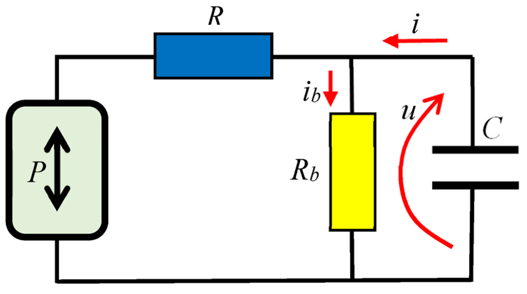
In contrast to the standard RC model, many research studies proposed using additional parallel resistance to characterize leakage currents (LCs) flowing in SCs. The charging current required to keep the SC voltage constant at a specified preset value is denoted by the LC. In manufacturers’ datasheets, LC is given as the value of charging current needed to keep the SC at rated voltage after it has been at rated voltage for 72 h at room temperature. Temperature, operational conditions, aging, and other factors alter LC over time [28].

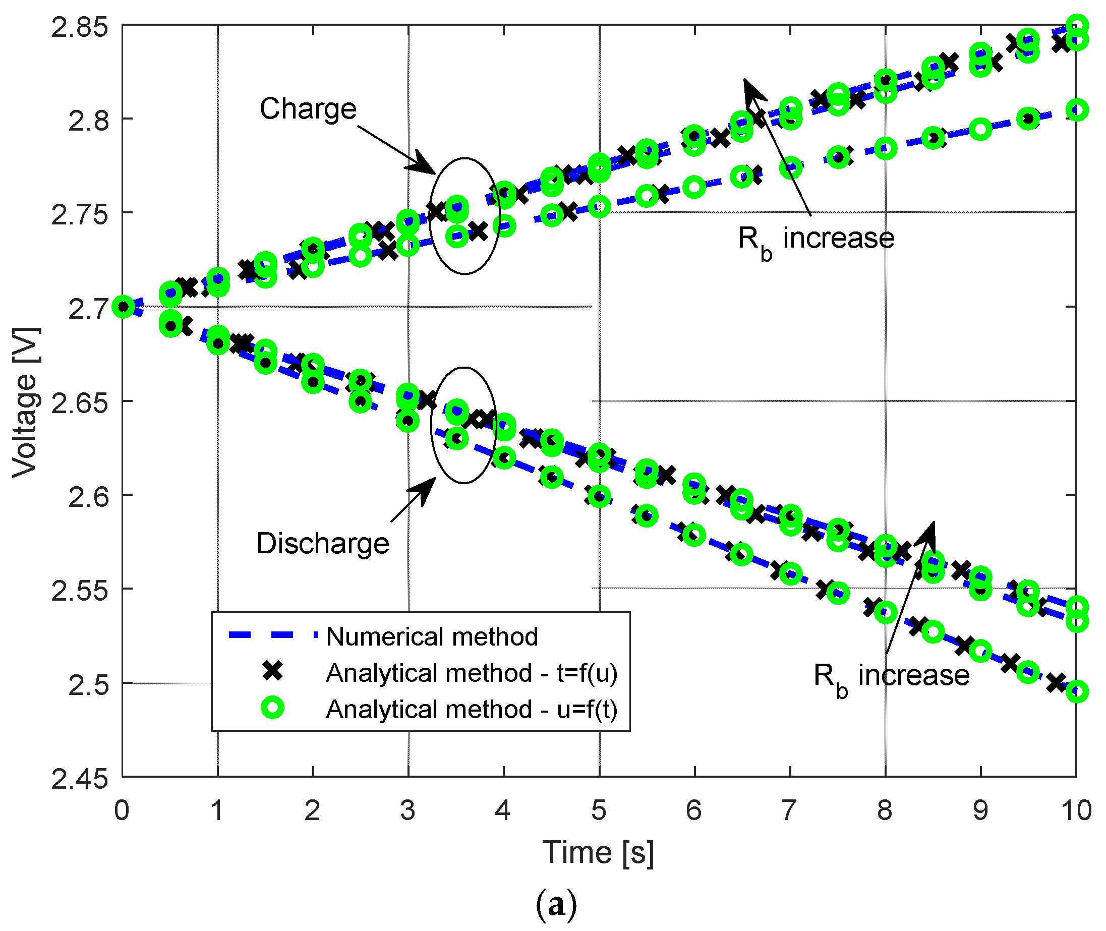
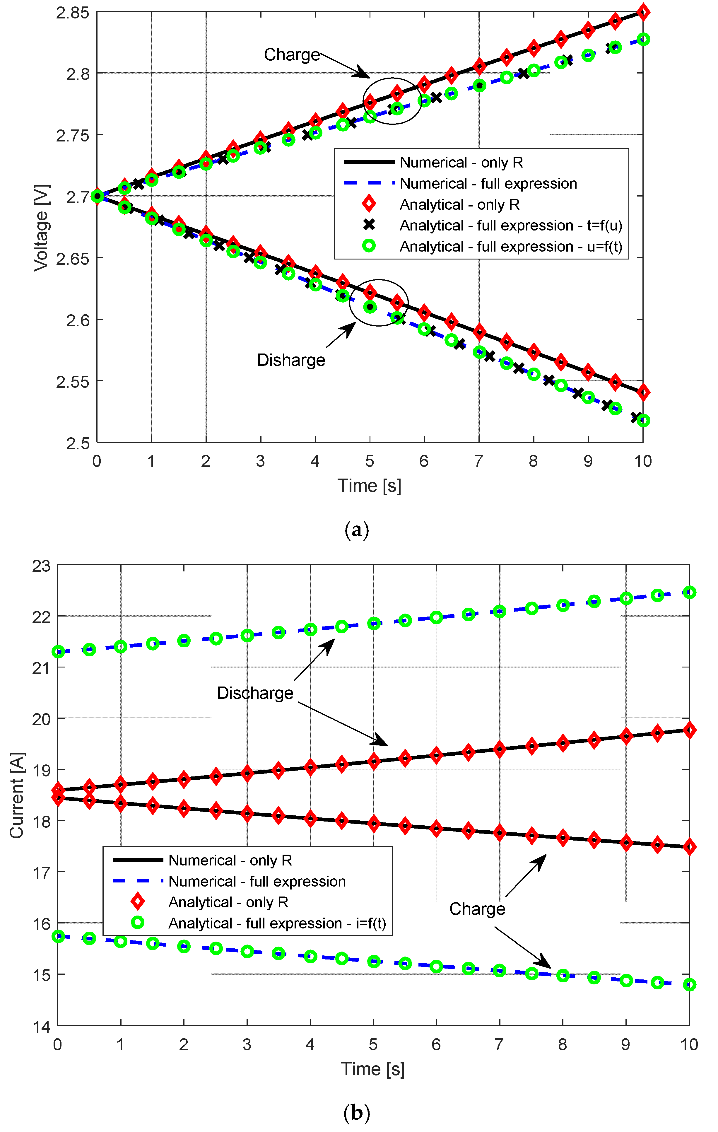
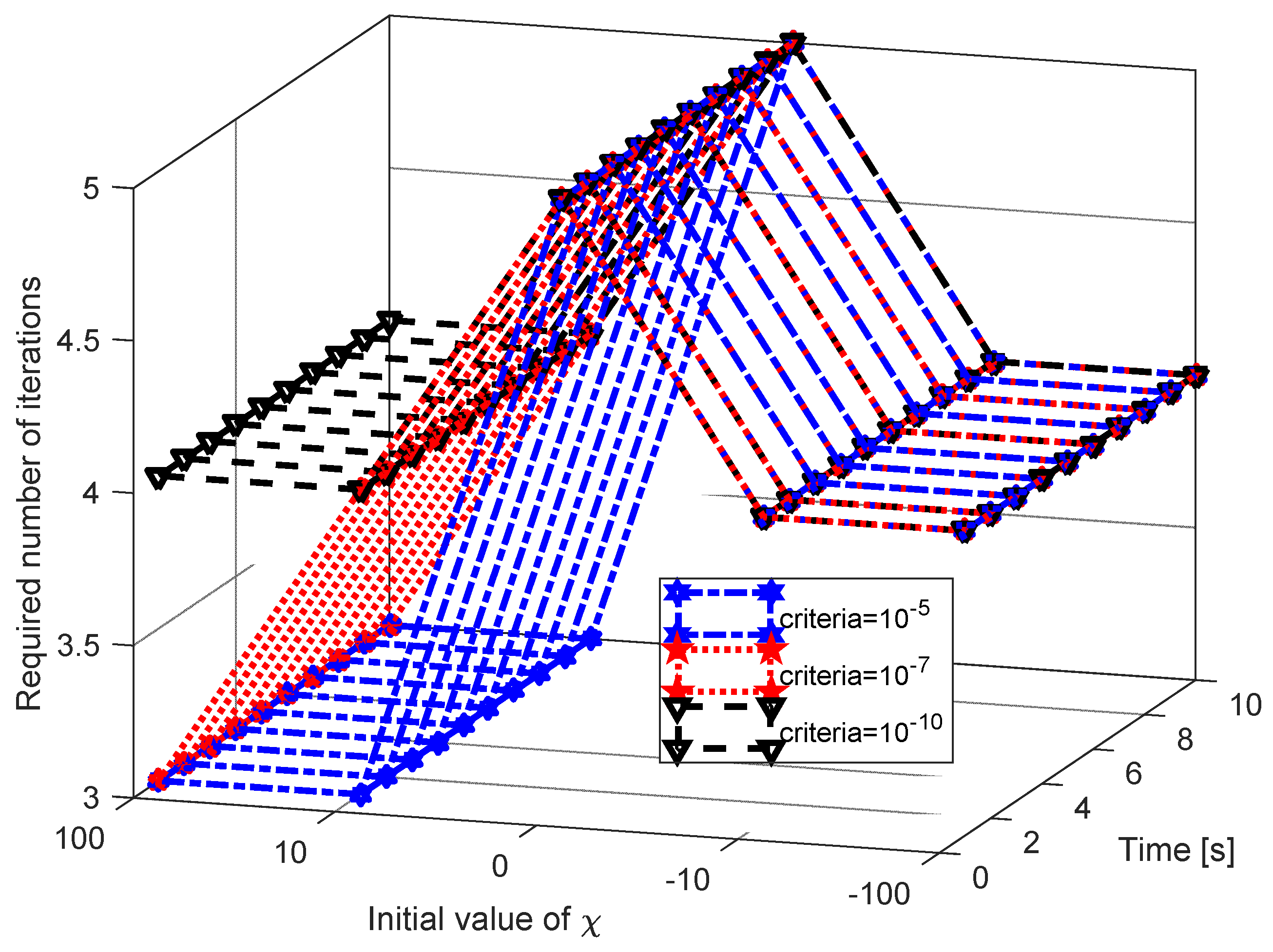
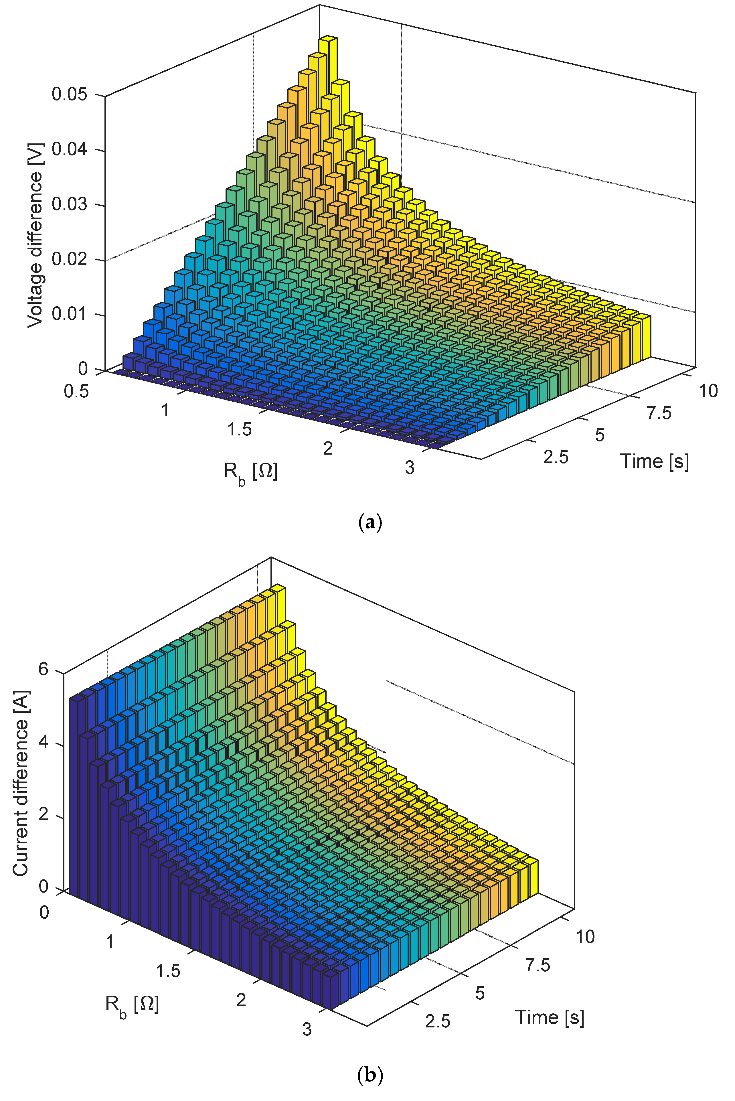
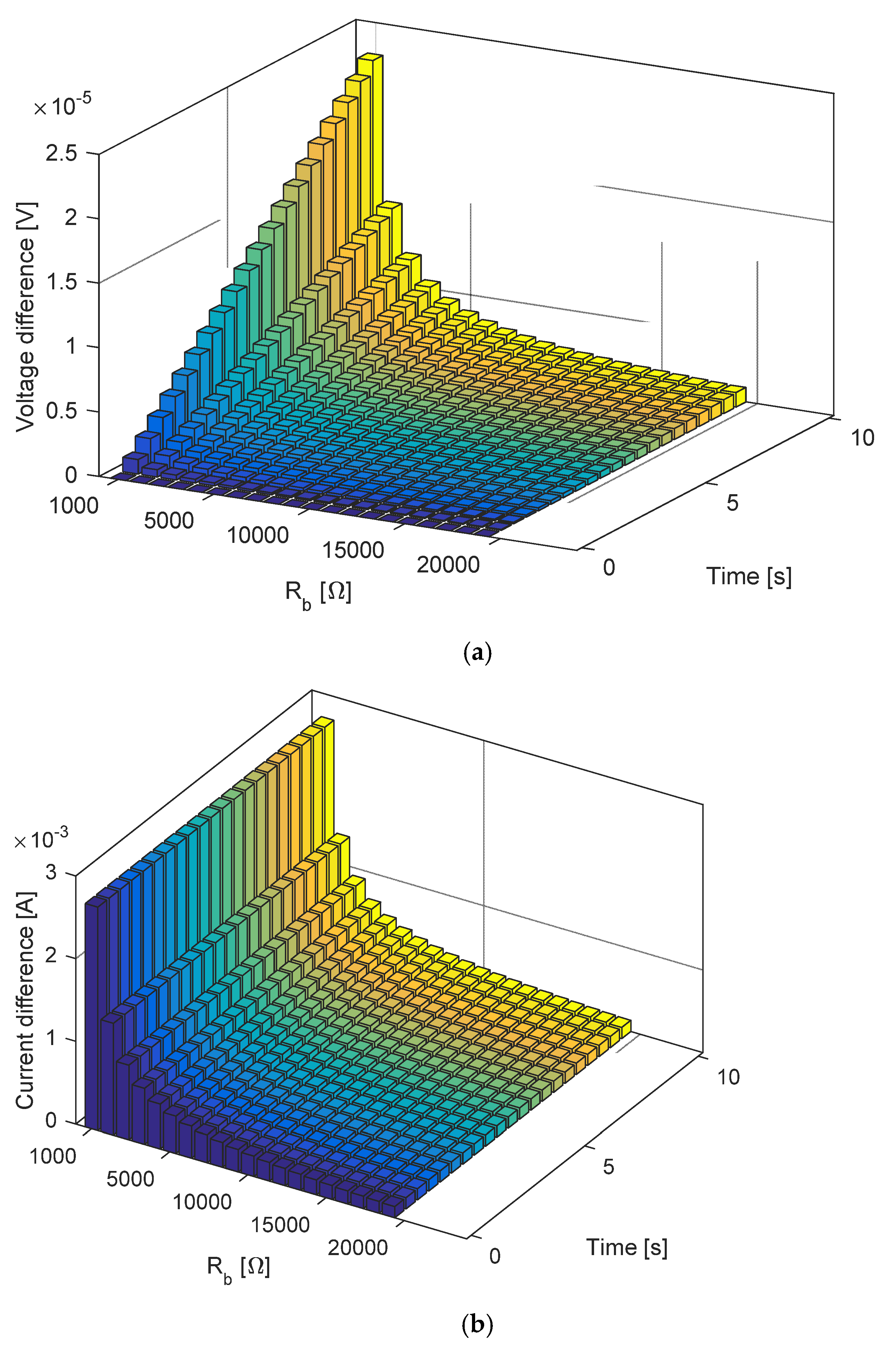
In this direction, this work provides a mathematical analysis of the current and voltage of SCs in the time domain, including a model of leakage current represented by parallel resistance at constant power. Consequently, this research is a continuation of analytical modeling of SC circuits that takes into account real effects during charging and discharging. The proposed analytical expressions make it possible to directly calculate the SC voltage and all currents in the SC model involved in charge/discharge processes as a function of time. In mathematical terms, the current-time and voltage-time can be expressed as a solution to a specific nonlinear equation, which is what Newton’s method is used to solve. The effect of parallel resistance is investigated by comparing the current-time and voltage-time curves of equivalent circuits with and without parallel resistance. The proposed expressions’ accuracy is compared with the results obtained using traditional methods based on numerical integration. A comparative analysis of the results is also presented; this determined when the leakage current effect is ignored.

The Newton method, also known as the Newton—Raphson method, is a popular iterative method for solving nonlinear equations. Over the years, various variants of the Newton method have been developed to address challenges in solving nonlinear equations, such as handling singular or ill-conditioned Jacobian matrices, improving the convergence rate and global behavior, and incorporating additional information such as constraints or second-order information.

Recent developments of the Newton method include globalized Newton methods to enhance the global convergence behavior, such as using trust-region or line-search strategies; inexact Newton methods to relax the accuracy requirement of the Jacobian matrix calculation, which can be more efficient for large-scale problems; Newton–Krylov methods to combine the Newton method with Krylov subspace methods, which can be more effective for sparse problems or problems with high dimensions; and parallel Newton methods to distribute the computation and communication of the Newton method across multiple processors to speed up the computation. The Newton method has been applied in various scientific communities, such as engineering, physics, economics, and computer science. Some examples of its applications include optimization—solving nonlinear optimization problems, such as finding the minimum of a function [29], dynamics—solving nonlinear ordinary or partial differential equations, such as modeling the motion of mechanical systems or fluid flows, data analysis—solving nonlinear inverse problems, such as estimating the parameters from observed data, and machine learning—solving nonlinear equations from machine learning models, such as deep neural networks or support vector machines. The literature shows improved versions of the standard Newton method [30,31,32]. For further details, a comparison of Newton–Raphson solvers for power flow problems is provided in [32].

The main paper contributions of this work are summarized as follows:

• In this paper, an accurate SC model is mathematically analyzed.
• The analytical expressions for current and voltage change via time are derived in both the charging and discharging processes.
• The comparison of results with and without the usage of parallel resistance in the SC model is investigated.
• The mathematical expressions derived for current and voltage are accurate and do not require any other mathematical formulations.

The structure of this article is as follows: Section 2 provides essential information regarding the mathematical modeling of SCs without leakage current. Section 3 offers the SC model with parallel resistance for the leaking current formulation and proposes a mathematical equation for modeling current and voltage analytically. In Section 4, simulation and numerical findings are provided. Conclusions are presented in Section 5.

2. Classic RC Model of Supercapacitors

The classic RC-based model of SCs used in constant power applications consists of a series connection of resistance R and capacitance C. The resistance represents thermal losses in this circuit caused by the current flow. This circuit is illustrated in Figure 1 [26,27].

The power balance equation of the classic RC-based model of SCs is given as follows [26]:

$$P+R{i}^2=ui$$

(1)

In Equation (1), u represents the voltage applied on the SC, while i represents the current flows in the circuit. The product ui represents the supercapacitor power, while Ri² represents the losses in the SC. If the power is positive, i.e., P > 0, it is a discharging process; otherwise, if the power is negative, i.e., P < 0, it is a charging process.

The current and voltage relation of the SC circuit is expressed as follows:

$$\frac{du}{dt}=-\frac{i}{C}$$

(2)

2.1. Pedrayes et al. Methods

The first Pedrayes et al. method was presented in [33]. For this method, the current calculation during the charging and discharging processes of a SC is given as follows:

$$i=P\sqrt{\frac{C}{\frac{C}{2}f\left(U_0\right)-2Pt}}$$

(3)

where

$$f\left(U_0\right)=U_0^2+U_0\sqrt{U_0^2-4RP}-2RP$$

(4)

where U₀ is the initial value of voltage u.

The second Pedrayes et al. method was presented in [26], in which they presented expressions of electrical variables of SCs during charging and discharging processes in constant power applications using the Lambert W function for the first time in the literature. These expressions are given as follows:

$$u=\sqrt{RP}\left(\sqrt{g_1}+\frac{1}{\sqrt{g_1}}\right)$$

(5)

$$i=\sqrt{\frac{P}{R{g}_1}}$$

(6)

where

$$g_1=-W_{-1}\left(\frac{-\exp \left(-\frac{g}{2RP}\right)}{2RP}\right)$$

(7)

so that

$$\begin{array}{l}g=h+2RP\left(\log \left(2\right)-1\right)\\ h=U_0^2+U_0\sqrt{U_0^2-4RP}-4RP\log \left(U_0\sqrt{U_0^2-4RP}\right)-\frac{4Pt}{C}\end{array}$$

(8)

In Equation (7), the second branch of the Lambert W function, noted with W₋₁, has been used. Mathematically, the principal branch should be used if the SC charges (P < 0). Detailed explanations, as well as the derivation of the equations, are given in [26].

2.2. Calasan et al. Method

In [27], Calasan et al. proposed analytical expressions for the discharge and charge processes in SCs using two transcendental equations (x = β∙exp(x) and x = β∙exp(−x)) with positive arguments.

The discharge current and voltage are represented as follows:

$$i=\sqrt{\frac{P}{R\mathsf{\Upsilon }}}$$

(9)

$$u=\sqrt{PR}\left(\frac{1+\mathsf{\Upsilon }}{\sqrt{\mathsf{\Upsilon }}}\right)$$

(10)

where $\mathsf{\Upsilon }$ denotes the solution of the transcendental equation, which is given in the following form:

$$\mathsf{\Upsilon }=\mathsf{\beta }\exp \left(\mathsf{\Upsilon }\right), \mathsf{\beta }>0$$

(11)

so that

$$\mathsf{\beta }=\frac{1}{4PR}\exp \left(1-\frac{U_0^2+U_0\sqrt{U_0^2-4PR}-4PR\log \left(U_0+\sqrt{U_0^2-4PR}\right)-\frac{4Pt}{C}}{2PR}\right)$$

(12)

During the charging process, the power P is negative and can be expressed as P₁ = −P. Thus, the mathematical expressions for current and voltage are expressed as follows:

$$i=\sqrt{\frac{P_1}{R\mathsf{\Psi }}}$$

(13)

$$u=\sqrt{P_{1}R}\left(\frac{\mathsf{\Psi }-1}{\sqrt{\mathsf{\Psi }}}\right)$$

(14)

where $\mathsf{\Psi }$ is the solution to the equation

$$\mathsf{\Psi }=\mathsf{\alpha }\exp \left(-\mathsf{\Psi }\right), \mathsf{\alpha }>0$$

(15)

so that

$$\mathsf{\alpha }=\frac{1}{4P_{1}R}\exp \left(1+\frac{U_0^2+U_0\sqrt{U_0^2+4P_{1}R}+4P_{1}R\log \left(U_0+\sqrt{U_0^2+4P_{1}R}\right)+\frac{4P_{1}t}{C}}{2P_{1}R}\right)$$

(16)

For all methods, the active power losses can be calculated as follows:

$$P_{loss}=R{i}^2$$

(17)

To summarize, both transcendental equations were solved analytically using the STFT [34]. The number of potential solutions of these equations was discussed, and their usage was also described. The reader can refer to [27,35] for more details about these equations and other problem-solving methods.

3. RC Model of Supercapacitors with Leakage Current: Description and Formulation Proposed

The model of a SC with leakage current represented via shunt resistance R_b is illustrated in Figure 2. This circuit was proposed in [28]. Unlike the classic SC model, this circuit comprised an additional shunt resistance R_b to formulate the leakage current. The simple method for calculating the shunt resistance value was presented, in which R_b defines the property of the SC to discharge even if it was not connected to a load.

The power balance equation of this model is expressed as follows:

$$P+R{\left(i-\frac{u}{R_b}\right)}^2+\frac{u^2}{R_b}=ui$$

(18)

For a theoretically large value of R_b, R_b→∞, this equation will be the same as Equation (1).

3.1. Discharge Process

In the discharge process, P > 0. In this case, Equation (18) can be rewritten in the following manner:

$$C\cdot \frac{du}{dt}=-\frac{u}{2R}-\frac{u}{R_b}+\frac{\sqrt{u^2-4RP}}{2R}$$

(19)

The solution to this equation is derived as follows:

$$t=t_0-CR{R}_b\left(\left(\frac{1}{2\left(R+R_b\right)}+\frac{1}{2R}\right)\log \left(\left(R+R_b\right){\left(u-\sqrt{u^2-4RP}\right)}^2+4R^{2}P\right)-\frac{1}{R}\log \left(u-\sqrt{u^2-4RP}\right)\right)$$

(20)

where

$$t_0=CR{R}_b\left(\left(\frac{1}{2\left(R+R_b\right)}+\frac{1}{2R}\right)\log \left(\left(R+R_b\right){\left(U_0-\sqrt{U_0^2-4RP}\right)}^2+4R^{2}P\right)-\frac{1}{R}\log \left(U_0-\sqrt{U_0^2-4RP}\right)\right)$$

(21)

Therefore, Equation (20) represents the function t = f(u). In order to define the relation between voltage and time, i.e., function u = f(t), one can derive the following:

$$\mathsf{\Lambda }=\mathsf{\chi }\cdot {\mathsf{\Lambda }}^{\mathsf{\delta }}+1,\mathsf{\delta }>1$$

(22)

where

$$\begin{array}{l}\mathsf{\delta }=\frac{2R+R_b}{R+R_b},\\ \mathsf{\chi }=\left(R+R_b\right)\cdot {\left(4R^{2}P\right)}^{\frac{R}{R+R_b}}\cdot e^{\frac{2\left(t-t_0\right)}{C{R}_b}}.\end{array}$$

(23)

Based on Equation (22), the voltage- and current-versus-time relation has the following expressions:

$$u=\frac{{\left(4R^{2}P\cdot \mathsf{\Lambda }\right)}^{\frac{2R+R_b}{R+R_b}}\cdot e^{\frac{2\left(t-t_0\right)}{C{R}_b}}+4RP}{2{\left(4R^{2}P\cdot \mathsf{\Lambda }\right)}^{\frac{2R+R_b}{2\left(R+R_b\right)}}\cdot e^{\frac{\left(t-t_0\right)}{C{R}_b}}}$$

(24)

$$\begin{array}{l}i=-\left(\frac{1}{2R}+\frac{1}{R_b}\right)\cdot \frac{{\left(4R^{2}P\cdot \mathsf{\Lambda }\right)}^{\frac{2R+R_b}{R+R_b}}\cdot e^{\frac{2\left(t-t_0\right)}{C{R}_b}}+4RP}{2{\left(4R^{2}P\cdot \mathsf{\Lambda }\right)}^{\frac{2R+R_b}{2\left(R+R_b\right)}}\cdot e^{\frac{\left(t-t_0\right)}{C{R}_b}}}+\\ \frac{1}{2R}\sqrt{{\left(\frac{{\left(4R^{2}P\cdot \mathsf{\Lambda }\right)}^{\frac{2R+R_b}{R+R_b}}\cdot e^{\frac{2\left(t-t_0\right)}{C{R}_b}}+4RP}{2{\left(4R^{2}P\cdot \mathsf{\Lambda }\right)}^{\frac{2R+R_b}{2\left(R+R_b\right)}}\cdot e^{\frac{\left(t-t_0\right)}{C{R}_b}}}\right)}^2-4RP}\end{array}$$

(25)

Finally, the leakage current has the following expression:

$$i_b=\frac{{\left(4R^{2}P\cdot \mathsf{\Lambda }\right)}^{\frac{2R+R_b}{R+R_b}}\cdot e^{\frac{2\left(t-t_0\right)}{C{R}_b}}+4RP}{2R_b\cdot {\left(4R^{2}P\cdot \mathsf{\Lambda }\right)}^{\frac{2R+R_b}{2\left(R+R_b\right)}}\cdot e^{\frac{\left(t-t_0\right)}{C{R}_b}}}$$

(26)

As seen, the expression for leakage current is, in a mathematical sense, equal to the expression for voltage. The only difference between these expressions is that the leakage current is u/R_b.

Finally, it is apparent that Equation (22) represents a nonlinear equation; one can use some iterative techniques, such as the Newton method, to solve it [30,31,32].

3.2. Charge Process

For charge process P < 0, one can assume P₁ = −P. In this case, the function t = f(u) has the following form:

$$t=CR{R}_b\left(\frac{1}{R}\log \left(\sqrt{u^2+4R{P}_1}-u\right)-\left(\frac{1}{2\left(R+R_b\right)}+\frac{1}{2R}\right)\log \left(\left(R+R_b\right){\left(\sqrt{u^2+4R{P}_1}-u\right)}^2-4R^2{P}_1\right)\right)-t_0$$

(27)

where

$$t_0=CR{R}_b\left(\frac{1}{R}\log \left(\sqrt{u_0^2+4R{P}_1}-u_0\right)-\left(\frac{1}{2\left(R+R_b\right)}+\frac{1}{2R}\right)\log \left(\left(R+R_b\right){\left(\sqrt{u_0^2+4R{P}_1}-u_0\right)}^2-4R^2{P}_1\right)\right)$$

(28)

In order to define the relationship between voltage and time, i.e., function u = f(t), the previous equation can be rewritten in the following form:

$$\mathsf{{\rm X}}=\mathsf{\xi }\cdot {\mathsf{{\rm X}}}^{\mathsf{\delta }}+1$$

(29)

so that;

$$\mathsf{\xi }=\left(R+R_b\right)\cdot {\left(4R^2{P}_1\right)}^{\frac{R}{R+R_b}}\cdot e^{\frac{2\left(t+t_0\right)}{C{R}_b}}$$

(30)

Based on this equation, the voltage- and current-versus-time relationship has the following expressions:

$$u=\frac{{\left(4R^2{P}_1\cdot \mathsf{{\rm X}}\right)}^{\frac{2R+R_b}{R+R_b}}\cdot e^{\frac{2\left(t+t_0\right)}{C{R}_b}}-4R{P}_1}{2{\left(4R^2{P}_1\cdot \mathsf{{\rm X}}\right)}^{\frac{2R+R_b}{2\left(R+R_b\right)}}\cdot e^{\frac{\left(t+t_0\right)}{C{R}_b}}}$$

(31)

$$i=-\left(\frac{1}{2R}+\frac{1}{R_b}\right)\cdot \frac{{\left(4R^2{P}_1\cdot \mathsf{{\rm X}}\right)}^{\frac{2R+R_b}{R+R_b}}\cdot e^{\frac{2\left(t+t_0\right)}{C{R}_b}}-4R{P}_1}{2{\left(4R^2{P}_1\cdot \mathsf{{\rm X}}\right)}^{\frac{2R+R_b}{2\left(R+R_b\right)}}\cdot e^{\frac{\left(t+t_0\right)}{C{R}_b}}}+\frac{1}{2R}\sqrt{{\left(\frac{{\left(4R^2{P}_1\cdot \mathsf{{\rm X}}\right)}^{\frac{2R+R_b}{R+R_b}}\cdot e^{\frac{2\left(t+t_0\right)}{C{R}_b}}-4R{P}_1}{2{\left(4R^2{P}_1\cdot \mathsf{{\rm X}}\right)}^{\frac{2R+R_b}{2\left(R+R_b\right)}}\cdot e^{\frac{\left(t+t_0\right)}{C{R}_b}}}\right)}^2+4R{P}_1}$$

(32)

Also, the leakage current has the following expression:

$$i_b=\frac{{\left(4R^2{P}_1\cdot \mathsf{{\rm X}}\right)}^{\frac{2R+R_b}{R+R_b}}\cdot e^{\frac{2\left(t+t_0\right)}{C{R}_b}}-4R{P}_1}{2R_b{\left(4R^2{P}_1\cdot \mathsf{{\rm X}}\right)}^{\frac{2R+R_b}{2\left(R+R_b\right)}}\cdot e^{\frac{\left(t+t_0\right)}{C{R}_b}}}$$

(33)

The active power losses (P_loss) can be calculated for both charge and discharge processes as follows:

$$P_{loss}=R{i}^2+R_b{i}_b^2$$

(34)

To summarize, expressions for calculating the current, voltage, power losses, and leakage current of the RC model of SCs with leakage current are derived.

4. Numerical Results Obtained and Their Discussion

4.1. Numerical Results Obtained

To test the accuracy of the derived expressions in the calculation of current and voltage as a function of the time of SCs when the effect of leakage currents is taken into account, the SC, whose basic parameters are presented in

Table 1. Data of the SC investigated in this study.

Parameter	Value
U0 (V)	2.7
C (kF)	1.2
R (mΩ)	0.58

, is investigated in this study. These SC data have also been used in previous research [26,27]. However, the effect of the leakage current was not considered.

Table 2. Numerical results calculated in SC discharging, R_b = 10 Ω.

t (s)	$\mathsf{\chi }$	$\mathsf{\Lambda }$	u (V)	i (A)	ib (A)
0.0	0.985500293824554	70.1423	2.7000	18.8628	0.2700
0.5	0.985582422271010	70.5505	2.6921	18.9168	0.2692
1.0	0.985664557561789	70.9634	2.6842	18.9713	0.2684
1.5	0.985746699697461	71.3813	2.6763	19.0263	0.2676
2.0	0.985828848678595	71.8042	2.6684	19.0817	0.2668
2.5	0.985911004505764	72.2322	2.6604	19.1377	0.2660
3.0	0.985993167179537	72.6653	2.6524	19.1942	0.2652
3.5	0.986075336700484	73.1038	2.6444	19.2512	0.2644
4.0	0.986157513069177	73.5476	2.6364	19.3088	0.2636
4.5	0.986239696286186	73.9968	2.6283	19.3668	0.2628
5.0	0.986321886352082	74.4517	2.6203	19.4255	0.2620
5.5	0.986404083267435	74.9122	2.6121	19.4846	0.2612
6.0	0.986486287032816	75.3785	2.6040	19.5444	0.2604
6.5	0.986568497648797	75.8507	2.5959	19.6047	0.2596
7.0	0.986650715115948	76.3289	2.5877	19.6655	0.2588
7.5	0.986732939434840	76.8133	2.5795	19.7270	0.2579
8.0	0.986815170606045	77.3038	2.5712	19.7891	0.2571
8.5	0.986897408630131	77.8008	2.5630	19.8517	0.2563
9.0	0.986979653507673	78.3042	2.5547	19.9150	0.2555
9.5	0.987061905239239	78.8142	2.5464	19.9790	0.2546
10.0	0.987144163825403	79.3310	2.5380	20.0435	0.2538

explores the results of calculating the current, voltage, and other values during discharging of the SC at small parallel resistance, R_b = 10 Ω and δ = 1.000057996636195 using P = 50 W, C = 1200 F, and R = 0.58 mΩ. In this case, we observed specific time values with a time step of 0.5 s to show the numerical value of all variables (voltage, current, leakage current). Likewise,

Table 3. Numerical results calculated in SC discharging, R_b = 1000 Ω.

t (s)	$\mathsf{\chi }$	$\mathsf{\Lambda }$·1000	u (V)	i (A)	ib (A)
0.0	0.999850256058536	6.9148	2.7000	18.5955	0.002700000000001
0.5	0.999851089267431	6.9551	2.6922	18.6495	0.002692240647929
1.0	0.999851922477020	6.9958	2.6845	18.7040	0.002684458692096
1.5	0.999852755687302	7.0370	2.6767	18.7589	0.002676653933216
2.0	0.999853588898279	7.0786	2.6688	18.8144	0.002668826169019
2.5	0.999854422109949	7.1208	2.6610	18.8704	0.002660975194265
3.0	0.999855255322315	7.1635	2.6531	18.9268	0.002653100800589
3.5	0.999856088535375	7.2067	2.6452	18.9838	0.002645202776528
4.0	0.999856921749130	7.2504	2.6373	19.0413	0.002637280907384
4.5	0.999857754963579	7.2947	2.6293	19.0993	0.002629334975200
5.0	0.999858588178722	7.3395	2.6214	19.1578	0.002621364758679
5.5	0.999859421394559	7.3848	2.6134	19.2169	0.002613370033081
6.0	0.999860254611090	7.4307	2.6054	19.2766	0.002605350570184
6.5	0.999861087828317	7.4772	2.5973	19.3368	0.002597306138192
7.0	0.999861921046237	7.5243	2.5892	19.3976	0.002589236501677
7.5	0.999862754264852	7.5720	2.5811	19.4589	0.002581141421454
8.0	0.999863587484160	7.6203	2.5730	19.5209	0.002573020654567
8.5	0.999864420704164	7.6692	2.5649	19.5834	0.002564873954097
9.0	0.999865253924862	7.7187	2.5567	19.6465	0.002556701069188
9.5	0.999866087146254	7.7689	2.5485	19.7103	0.002548501744906
10.0	0.999866920368341	7.8198	2.5403	19.7747	0.002540275722114

explores the results obtained at considerable parallel resistance, R_b = 1000 Ω and δ = 1.00000579999664. Analog results in the SC charging process are presented in

Table 4. Numerical results calculated in SC charging, R_b = 10 Ω.

t (s)	$\mathit{\xi }$	X	u (V)	i (A)	ib (A)
0.0	1.014666570664325	67.0507	2.7000	18.1754	0.2700
0.5	1.014751129735126	66.6741	2.7076	18.1236	0.2708
1.0	1.014835695852810	66.3016	2.7151	18.0721	0.2715
1.5	1.014920269017964	65.9333	2.7226	18.0211	0.2723
2.0	1.015004849231176	65.5689	2.7301	17.9705	0.2730
2.5	1.015089436493032	65.2086	2.7376	17.9203	0.2738
3.0	1.015174030804120	64.8521	2.7451	17.8705	0.2745
3.5	1.015258632165028	64.4995	2.7525	17.8211	0.2752
4.0	1.015343240576344	64.1506	2.7599	17.7721	0.2760
4.5	1.015427856038654	63.8055	2.7673	17.7235	0.2767
5.0	1.015512478552546	63.4640	2.7747	17.6753	0.2775
5.5	1.015597108118608	63.1262	2.7820	17.6274	0.2782
6.0	1.015681744737428	62.7918	2.7894	17.5800	0.2789
6.5	1.015766388409594	62.4610	2.7967	17.5329	0.2797
7.0	1.015851039135692	62.1336	2.8040	17.4861	0.2804
7.5	1.015935696916312	61.8096	2.8113	17.4398	0.2811
8.0	1.016020361752041	61.4889	2.8185	17.3937	0.2819
8.5	1.016105033643467	61.1715	2.8257	17.3481	0.2826
9.0	1.016189712591178	60.8573	2.8330	17.3027	0.2833
9.5	1.016274398595761	60.5463	2.8402	17.2578	0.2840
10.0	1.016359091657807	60.2384	2.8473	17.2131	0.2847

and

Table 5. Numerical results calculated in SC charging, R_b = 1000 Ω.

t (s)	$\mathit{\xi }$	X∙1000	u (V)	i (A)	ib (A)
0.0	1.000141859861932	6.8037	2.7000	18.4427	0.002700000000007
0.5	1.000142693313829	6.7655	2.7077	18.3909	0.002707673649208
1.0	1.000143526766421	6.7277	2.7153	18.3394	0.002715325775111
1.5	1.000144360219706	6.6903	2.7230	18.2884	0.002722956557277
2.0	1.000145193673687	6.6534	2.7306	18.2378	0.002730566172834
2.5	1.000146027128362	6.6168	2.7382	18.1876	0.002738154796433
3.0	1.000146860583733	6.5807	2.7457	18.1379	0.002745722600371
3.5	1.000147694039798	6.5449	2.7533	18.0885	0.002753269754584
4.0	1.000148527496555	6.5095	2.7608	18.0396	0.002760796426700
4.5	1.000149360954010	6.4745	2.7683	17.9910	0.002768302782151
5.0	1.000150194412157	6.4399	2.7758	17.9428	0.002775788984090
5.5	1.000151027871000	6.4056	2.7833	17.8950	0.002783255193553
6.0	1.000151861330537	6.3718	2.7907	17.8476	0.002790701569405
6.5	1.000152694790770	6.3382	2.7981	17.8006	0.002798128268451
7.0	1.000153528251695	6.3050	2.8055	17.7539	0.002805535445412
7.5	1.000154361713316	6.2722	2.8129	17.7076	0.002812923253052
8.0	1.000155195175632	6.2397	2.8203	17.6617	0.002820291842097
8.5	1.000156028638642	6.2075	2.8276	17.6161	0.002827641361340
9.0	1.000156862102347	6.1757	2.8350	17.5708	0.002834971957704
9.5	1.000157695566744	6.1442	2.8423	17.5259	0.002842283776184
10.0	1.000158529031839	6.1130	2.8496	17.4814	0.002849576959995

, respectively.

Additionally, the impacts of the parallel resistance value on the current, voltage, and leakage current are visualized in Figure 3 for different parallel resistance values, in which the results determined using the expressions proposed in this study are compared with corresponding ones determined using numerical integration, with integration step size 10⁻⁵. For such comparison, the following set of differential equations was used:

$$\begin{array}{l}\frac{du}{dt}=-\frac{u}{2RC}-\frac{u}{R_{b}C}+\frac{\sqrt{u^2-4RP}}{2RC},\\ i=-C\cdot u^{\prime },\\ i_b=\frac{u}{R_b}.\end{array}$$

(35)

One can draw several conclusions based on the results in Table 2, Table 3, Table 4 and Table 5. Namely, the values of the $\mathsf{\delta }$ coefficient are close to 1. The coefficient values $\mathsf{\chi }$ in the discharging process (or coefficient $\mathsf{\xi }$ in the charging process) are very close and only differ by some decimals; however, this difference greatly affects the value of $\mathsf{\Lambda }$ in the discharging process (or the value of X in the charging process). Accordingly, even a small change in $\mathsf{\chi }$ or $\mathsf{\xi }$ values could dramatically impact the voltage and current values of SCs.

It can be seen from the presented results that higher values of parallel resistance result in a lower value of self-discharge current. Three resistance values are shown on these graphs, and small values of parallel resistance (0.5, 3, and 100 ohms) are considered, to show their effects on current and voltage values. During the discharge process, the SC voltage increases, while the current decreases, with higher parallel resistance values. The opposite situation will occur during the charging of the SC.

Furthermore, a comparison of the current-time and voltage-time characteristics obtained by applying the derived expressions with the corresponding characteristics obtained by ignoring the effect of the parallel resistance (i.e., considering R_b →∞) is shown in Figure 4. In this case, it is assumed that the value of parallel resistance is minimal, to provide a much more apparent impact on the characteristics. The characteristics obtained by applying the expressions t = f(u) and u = f(t) are also shown for voltage-time characteristics.

Based on the presented results, for both modes of operation, it is clear that the derived expressions t = f(u), u = f(t), as well as i = f(t), are accurate and precise. Characteristics obtained at the neglected value of parallel resistance were determined using the Calasan et al. method [27]. The corresponding characteristics obtained numerically are determined by solving the following system of equations:

$$\begin{array}{l}\frac{du}{dt}=-\frac{u}{2RC}+\frac{\sqrt{u^2-4RP}}{2RC}\\ i=-C\cdot u^{\prime }\end{array}$$

(36)

In order to check the influence of the initial conditions on the speed of convergence of the Newton method, the calculation results were repeated for five different initial condition values (–100, –10, 0, 10, and 100). Moreover, the convergence rate was tested for three different values of the convergence criteria: 10⁻⁵, 10⁻⁷, and 10⁻¹⁰. The criterion is defined as the absolute value of the difference between two neighboring variable values $\mathsf{\Lambda }$ during the iterative process. This test was done for the case of the results shown in Table 2 (SC discharge, discharge power is 50 W, parallel resistance is 10 Ω). Figure 5 shows the influence of the initial conditions on the speed of convergence of the Newton method and the number of iterations in the problem solved.

Based on the obtained results, it can be observed that the Newton method converges very quickly for a different starting value of the variable $\mathsf{\Lambda }$. Moreover, the convergence criterion has little impact on the convergence speed.

Seeking additional validation, the impact of the parallel resistance R_b value on the voltage-time and current-time characteristics is also analyzed using a 3D graph presented in Figure 6 and Figure 7 for small and large values of R_b, respectively, during the charging process. These figures illustrate the differences in voltages and currents calculated using the full expression derived in this paper and the Calasan et al. method [27] with infinite parallel resistance value.

From Figure 7, it is clear that for the small value of the parallel resistance, there is an evident difference between current and voltage calculations when comparing the entire model and the simple model (parallel resistance ignored), and it rises for the smaller values of the parallel resistance R_b.

From Figure 7, it is clear that the mentioned difference exists, but it is very small and tends to zero for large values of parallel resistance. To sum up, considerable parallel resistance values result in a much more negligible difference between characteristics determined with and without parallel resistance. However, these differences are much more prominent for both current and voltage for smaller R_b values (Figure 6).

4.2. Parametric Variations

4.2.1. Power Variation

Figure 8 illustrates how power affects the voltage-time, current-time, and leakage-current-time characteristics in the discharging mode. A higher power value indicates a quicker drop in voltage and leakage current when a larger current is present.

4.2.2. Capacitance Variation

The impact of capacitance on voltage-time, current-time, and leakage current-time characteristics in the charging mode of the SC is shown in Figure 9. A higher capacitance value defines a slower voltage and leakage-current-value growth and slower current decrease.

4.2.3. Effect of Successive Changes in the Charging and Discharging Power

Finally, the impact of consecutive modifications to the SC’s charging and discharging power on voltage-time, current-time, and leakage-current-time characteristics were examined. The corresponding graphs are shown in Figure 10. In order to clearly observe the effect of the parallel resistance, it was set to a small value (R_b = 1 ohm).

Based on the findings, it is evident that the voltage differences between those obtained by using the derived expression and those obtained by using the expression given in the literature by Calasan et al. [27]—which ignores the effects of parallel resistance and self-discharge current—increase over time. The SC voltage decreases for a positive power value when the current increases. Moreover, the opposite is valid for negative power values. A larger positive/negative power value results in larger voltage and current changes.

5. Conclusions

This study provides accurate analytical formulas for leakage-current-based SC models used in industrial applications, i.e., applications based on constant power and incorporating leakage currents of SCs. The suggested model expresses current and voltage as nonlinear equations solved using Newton’s method. The accuracy of the suggested expressions is compared to the results generated with traditional techniques based on numerical integration. It also includes a comparison of the results derived when the effect of the leakage current is disregarded. The outcomes demonstrate that using leakage current in SC modeling provides a more accurate and realistic approach. The derived formulas for the representation of voltage, current, and leakage current of SCs as a function of time permit perfect agreement with the corresponding findings obtained by applying numerical integration as inferred based on all the results that have been provided. As a result, the terms that were derived can be used to describe how SCs are charged and discharged, to analyze the operating mode, to look at the effects of specific parameters on current and voltage, to test their use in regulated systems, or to test protection against excessive currents or voltage. Additionally, the fields of application of the solution methodology proposed are flexible.

In future work, attention will be paid to implementing the proposed model in a whole system with all components, such as in renewable power generation and control system. Furthermore, attention will be paid to the analytical solution of the proposed nonlinear equation to improve existing research based on the Newton method while considering global convergence strategies to enhance the convergence robustness.

References

1. Yamashita, K.; Villanueva, S.M. Integration of renewable energy sources, energy storages, and their impacts. In Encyclopedia of Electrical and Electronic Power Engineering; García, J., Ed.; Elsevier: Oxford, UK, 2023; pp. 36–44. ISBN 978-0-12-823211-8. [Google Scholar]
2. Ćalasan, M.; Abdel Aleem, S.H.E.; Hasanien, H.M.; Alaas, Z.M.; Ali, Z.M. An innovative approach for mathematical modeling and parameter estimation of PEM fuel cells based on iterative Lambert W function. Energy 2023, 264, 126165. [Google Scholar] [CrossRef]
3. Ebeed, M.; Aleem, S.H.E.A. Overview of uncertainties in modern power systems: Uncertainty models and methods. In Uncertainties in Modern Power Systems; Elsevier: Amsterdam, The Netherlands, 2021; pp. 1–34. [Google Scholar]
4. Michaelides, E.E.; Nguyen, V.N.D.; Michaelides, D.N. The effect of electric vehicle energy storage on the transition to renewable energy. Green Energy Intell. Transp. 2023, 2, 100042. [Google Scholar] [CrossRef]
5. Zhang, D.; Shafiullah, G.M.; Das, C.K.; Wong, K.W. A systematic review of optimal planning and deployment of distributed generation and energy storage systems in power networks. J. Energy Storage 2022, 56, 105937. [Google Scholar] [CrossRef]
6. Ćalasan, M.; Kecojević, K.; Lukačević, O.; Ali, Z.M. Testing of influence of SVC and energy storage device’s location on power system using GAMS. In Uncertainties in Modern Power Systems; Elsevier: Amsterdam, The Netherlands, 2021; pp. 297–342. [Google Scholar]
7. Beires, P.; Vasconcelos, M.H.; Moreira, C.L.; Peças Lopes, J.A. Stability of autonomous power systems with reversible hydro power plants: A study case for large scale renewables integration. Electr. Power Syst. Res. 2018, 158, 1–14. [Google Scholar] [CrossRef]
8. Lu, Z. Experimental analysis of one micro-compressed air energy storage-power generation system with different working fluids. J. Energy Storage 2023, 60, 106647. [Google Scholar] [CrossRef]
9. Billings, B.W.; Ho, A.; Sahraei-Adrakani, M.; Powell, K.M. System benefits of industrial battery storage: A comparison of grid and facility control and dispatch. Sustain. Energy Grids Netw. 2022, 32, 100958. [Google Scholar] [CrossRef]
10. Mahdy, A.; Hasanien, H.M.; Turky, R.A.; Abdel Aleem, S.H.E. Modeling and optimal operation of hybrid wave energy and PV system feeding supercharging stations based on golden jackal optimal control strategy. Energy 2023, 263, 125932. [Google Scholar] [CrossRef]
11. Li, Z.; Song, K.; Jiang, J.; Zhu, C. Constant Current Charging and Maximum Efficiency Tracking Control Scheme for Supercapacitor Wireless Charging. IEEE Trans. Power Electron. 2018, 33, 9088–9100. [Google Scholar] [CrossRef]
12. Musolino, V.; Piegari, L.; Tironi, E. New full-frequency-range supercapacitor model with easy identification procedure. IEEE Trans. Ind. Electron. 2013, 60, 112–120. [Google Scholar] [CrossRef]
13. Zhang, L.; Hu, X.; Wang, Z.; Sun, F.; Dorrell, D.G. A review of supercapacitor modeling, estimation, and applications: A control/management perspective. Renew. Sustain. Energy Rev. 2018, 81, 1868–1878. [Google Scholar] [CrossRef]
14. Deng, Y.; Li, C.; Deng, Y.; Chen, T.; Feng, S.; Chu, Y.; Li, C. Energy Efficiency Optimization of Collaborative Power Supply System with Supercapacitor Storages. Energies 2023, 16, 1227. [Google Scholar] [CrossRef]
15. Molina-Ibáñez, E.L.; Rosales-Asensio, E.; Pérez-Molina, C.; Pérez, F.M.; Colmenar-Santos, A. Analysis on the electric vehicle with a hybrid storage system and the use of Superconducting magnetic energy storage (SMES). Energy Rep. 2021, 7, 854–873. [Google Scholar] [CrossRef]
16. Hannan, M.A.; Abu, S.M.; Al-Shetwi, A.Q.; Mansor, M.; Ansari, M.N.M.; Muttaqi, K.M.; Dong, Z.Y. Hydrogen energy storage integrated battery and supercapacitor based hybrid power system: A statistical analysis towards future research directions. Int. J. Hydrog. Energy 2022, 47, 39523–39548. [Google Scholar] [CrossRef]
17. Grbovic, P.J.; Delarue, P.; Le Moigne, P.; Bartholomeus, P. Modeling and Control of the Ultracapacitor-Based Regenerative Controlled Electric Drives. IEEE Trans. Ind. Electron. 2011, 58, 3471–3484. [Google Scholar] [CrossRef]
18. Gyawali, N.; Ohsawa, Y. Integrating fuel cell/electrolyzer/ultracapacitor system into a stand-alone microhydro plant. IEEE Trans. Energy Convers. 2010, 25, 1092–1101. [Google Scholar] [CrossRef]
19. Zhang, L.; Hu, X.; Wang, Z.; Sun, F.; Deng, J.; Dorrell, D.G. Multiobjective Optimal Sizing of Hybrid Energy Storage System for Electric Vehicles. IEEE Trans. Veh. Technol. 2018, 67, 1027–1035. [Google Scholar] [CrossRef]
20. Zhao, C.; Yin, H.; Yang, Z.; Ma, C. Equivalent series resistance-based energy loss analysis of a battery semiactive hybrid energy storage system. IEEE Trans. Energy Convers. 2015, 30, 1081–1091. [Google Scholar] [CrossRef]
21. Rawa, M.; Alghamdi, S.; Milyani, A.H.; Hariri, F.; Alghamdi, B.; Ajour, M.; Ćalasan, M.; Ali, Z.M.; Hasanien, H.M.; Popovic, B.; et al. Thermal model of supercapacitors operating in constant power applications: New mathematical expressions for precise calculation of temperature change. J. Energy Storage 2022, 49, 104121. [Google Scholar] [CrossRef]
22. Fouda, M.E.; Allagui, A.; Elwakil, A.S.; Eltawil, A.; Kurdahi, F. Supercapacitor discharge under constant resistance, constant current and constant power loads. J. Power Sources 2019, 435, 226829. [Google Scholar] [CrossRef]
23. Ahmad, F.F.; Ghenai, C.; Hamid, A.K.; Bettayeb, M. Application of sliding mode control for maximum power point tracking of solar photovoltaic systems: A comprehensive review. Annu. Rev. Control 2020, 49, 173–196. [Google Scholar] [CrossRef]
24. Sedaghat, M.; Siadatan, A.; Taheri, B. Photovoltaic Systems with Sliding Mode Control for Working in Maximum Power Point. Comput. Intell. Electr. Eng. 2018, 9, 77–90. [Google Scholar] [CrossRef]
25. Elwakil, A.S.; Allagui, A.; Maundy, B.J.; Psychalinos, C. A low frequency oscillator using a super-capacitor. AEU Int. J. Electron. Commun. 2016, 70, 970–973. [Google Scholar] [CrossRef]
26. Pedrayes, J.F.; Melero, M.G.; Cano, J.M.; Norniella, J.G.; Duque, S.B.; Rojas, C.H.; Orcajo, G.A. Lambert W function based closed-form expressions of supercapacitor electrical variables in constant power applications. Energy 2021, 218, 119364. [Google Scholar] [CrossRef]
27. Ćalasan, M.; Zobaa, A.F.; Hasanien, H.M.; Abdel Aleem, S.H.E.; Ali, Z.M. Towards accurate calculation of supercapacitor electrical variables in constant power applications using new analytical closed-form expressions. J. Energy Storage 2021, 42, 102998. [Google Scholar] [CrossRef]
28. Christen, T.; Carlen, M.W. Theory of ragone plots. J. Power Sources 2000, 91, 210–216. [Google Scholar] [CrossRef]
29. Zobaa, A.F.; Aleem, S.H.E.A.; Abdelaziz, A.Y. Classical and Recent Aspects of Power System Optimization; Academic Press: Cambridge, MA, USA, 2018; ISBN 9780128124420. [Google Scholar]
30. Aulisa, E.; Bnà, S.; Bornia, G. A monolithic ALE Newton–Krylov solver with Multigrid-Richardson–Schwarz preconditioning for incompressible Fluid-Structure Interaction. Comput. Fluids 2018, 174, 213–228. [Google Scholar] [CrossRef]
31. Zhang, H.; Guo, J.; Lu, J.; Niu, J.; Li, F.; Xu, Y. The comparison between nonlinear and linear preconditioning JFNK method for transient neutronics/thermal-hydraulics coupling problem. Ann. Nucl. Energy 2019, 132, 357–368. [Google Scholar] [CrossRef]
32. Sereeter, B.; Vuik, C.; Witteveen, C. On a comparison of Newton–Raphson solvers for power flow problems. J. Comput. Appl. Math. 2019, 360, 157–169. [Google Scholar] [CrossRef]
33. Pedrayes, J.F.; Melero, M.G.; Norniella, J.G.; Cano, J.M.; Cabanas, M.F.; Orcajo, G.A.; Rojas, C.H. A novel analytical solution for the calculation of temperature in supercapacitors operating at constant power. Energy 2019, 188, 116047. [Google Scholar] [CrossRef]
34. Rawa, M.; Al-Turki, Y.; Sindi, H.; Ćalasan, M.; Ali, Z.M.; Abdel Aleem, S.H.E. Current-voltage curves of planar heterojunction perovskite solar cells—Novel expressions based on Lambert W function and Special Trans Function Theory. J. Adv. Res. 2022, 44, 91–108. [Google Scholar] [CrossRef] [PubMed]
35. Ćalasan, M.; Abdel Aleem, S.H.E.; Zobaa, A.F. A new approach for parameters estimation of double and triple diode models of photovoltaic cells based on iterative Lambert W function. Sol. Energy 2021, 218, 392–412. [Google Scholar] [CrossRef]
Figure 1. Discharging of a SC at constant power P.
Energies 16 01903 g001
Figure 2. Discharging of a SC at constant power P, considering the leakage current.
Energies 16 01903 g002
Figure 3. Charging and discharging characteristics of a SC at constant power using different parallel resistance values: (a) voltage versus time; (b) current versus time; (c) leakage current versus time.
Energies 16 01903 g003aEnergies 16 01903 g003b
Figure 4. Characteristics of the SC at constant power determined using different methods during both charging and discharging processes (Rb = 1 Ω, P = 50 W, and C = 1200 F, and R = 0.58 mΩ): (a) voltage versus time; (b) current versus time.
Energies 16 01903 g004
Figure 5. Influence of the initial conditions on the speed of convergence of the Newton method and the number of iterations in the problem solved.
Energies 16 01903 g005
Figure 6. Differences in values of (a) voltages, and (b) currents, calculated using full expression derived in this study for small values of Rb and the Calasan et al. method in [27], with infinite parallel resistance value, considering P = 50 W, and R = 0.58 mΩ.
Energies 16 01903 g006
Figure 7. Differences in values of (a) voltages, and (b) currents, calculated using full expression derived in this study for large values of Rb and the Calasan et al. method in [27], with infinite parallel resistance value, considering P = 50 W, and R = 0.58 mΩ.
Energies 16 01903 g007
Figure 8. Discharging mode characteristics at different power values: (a) voltage versus time; (b) current versus time; (c) leakage current versus time; C = 1200 F, Rb = 1000 Ω, and R = 0.58 mΩ.
Energies 16 01903 g008aEnergies 16 01903 g008b
Figure 9. Charging mode characteristics at different capacitance values: (a) voltage versus time; (b) current versus time; (c) leakage current versus time; P = 50 W, Rb = 1000 Ω, and R = 0.58 mΩ.
Energies 16 01903 g009aEnergies 16 01903 g009b
Figure 10. Results obtained by using the derived expressions and those obtained by using the expressions presented in [27]: (a) successive power changes versus time; (b) voltage versus time; (c) current versus time; (d) difference between voltage calculated using the methods investigated; C = 1200 F, Rb = 1 Ω, and R = 0.58 mΩ.
Energies 16 01903 g010aEnergies 16 01903 g010b