Regional Load Frequency Control of BP-PI Wind Power Generation Based on Particle Swarm Optimization

Abstract

The large-scale integration of wind turbines (WTs) in renewable power generation induces power oscillations, leading to frequency aberration due to power unbalance. Hence, in this paper, a secondary frequency control strategy called load frequency control (LFC) for power systems with wind turbine participation is proposed. Specifically, a backpropagation (BP)-trained neural network-based PI control approach is adopted to optimize the conventional PI controller to achieve better adaptiveness. The proposed controller was developed to realize the timely adjustment of PI parameters during unforeseen changes in system operation, to ensure the mutual coordination among wind turbine control circuits. In the meantime, the improved particle swarm optimization (IPSO) algorithm is utilized to adjust the initial neuron weights of the neural network, which can effectively improve the convergence of optimization. The simulation results demonstrate that the proposed IPSO-BP-PI controller performed evidently better than the conventional PI controller in the case of random load disturbance, with a significant reduction to near 10 s in regulation time and a final stable error of less than ${10}^{-3}$ for load frequency. Additionally, compared with the conventional PI controller counterpart, the frequency adjustment rate of the IPSO-BP-PI controller is significantly improved. Furthermore, it achieves higher control accuracy and robustness, demonstrating better integration of wind energy into traditional power systems.

1. Introduction

With the increasing energy crisis and environmental pollution of today’s society, the development of renewable energy resources is gradually gaining attention all over the world. Wind energy is gradually recognized as one of the most essential and promising energy sources due to its advantages of clean environmental protection and high feasibility [1,2]. While wind power penetration gradually increases, its volatility and unpredictability bring great challenges to the stable operation of the wind power system. Compared with traditional thermal generating units, the method of using wind turbine units to provide electric power can often quickly respond to the change in load frequency. In addition, it is more suitable to achieve the frequency regulation of the power system. Therefore, it is crucial to explore an advanced control strategy to address the negative effects of load frequency fluctuation.

In order to realize stable load frequency control (LFC) for power systems with wind turbine integration and effectively improve the frequency regulation capability of wind power regions, researchers have carried out extensive research in related fields and have achieved a series of advanced results [3,4,5,6,7,8,9]. In [3], the authors proposed a robust control strategy based on equivalent input disturbance (EID) that uses equivalent input disturbance to compensate the imbalance between power generation and load. This improves the anti-disturbance performance of the power system in wind farms. However, at present, robust control cannot be accurately guaranteed to work in the optimal state for a long time [4]. Considering the existence of multiple energy sources serving local areas, the whale optimization algorithm (WOA) is used to optimize fuzzy integral PI controllers (FIPIs); then, the LFC problem in some regions and all regions in the interconnected power system of heat–water–wind areas are analyzed under the condition of sudden disturbance, which proves the superiority of the control method [5]. Additionally, an $H_2$/$H_{\infty }$ load frequency robust multi-objective TS fuzzy control method is applied in multi-area interconnected power systems, and a distributed compensation scheme is used to design the entire control system. Simulation data results show the robustness and effectiveness of this method when dealing with load disturbance, model uncertainty, transmission delay, and model nonlinear influence [4]. In [6], an ANFIS controller with artificial neural network was designed considering the strength of the nonlinear characteristics of doubly fed induction (DFIG) wind turbines and was successfully applied to the wind power generation system in two regions. The simulation results show that the controller was helpful in reducing overkill and shortening the regulation time of the nonlinear wind power generation system. The study [7] designed a load frequency controller based on PSO-MPC, which not only solved the randomness of wind turbine generation but also reduced the complexity of traditional MPC calculation, with fast response speed and high stability. However, this control method requires high precision of the model, and its continuous stability cannot be guaranteed. To achieve better system performance, the sliding mode control (SMC) strategy was used to analyze the frequency deviation and tie line power change of the interconnected power system in two regions under the disturbance of a fixed load, and a comparison with the traditional integral controller was made. The results show that the control method improved the response of the main loop to a great extent and that the frequency control effect was evident in case of overshoot and undershoot. Moreover, it can be widely used in situations where wind and conventional power generation work together [8]. The study [9] applied an optimal fuzzy PID sagging controller with adaptive and self-tuning functions to the structure of wind turbines, which effectively compensated for the decrease in the total inertia of the power system with the participation of the wind farm. At the same time, the artificial bee colony algorithm was used to optimize the membership function of input and output signals based on the multi-objective function. The simulation results show that the control method is reasonable, with short stabilizing time and high frequency control precision. In the paper [10], the researchers presented a data-driven and model-free frequency control method based on deep reinforcement learning (DRL) in the continuous-motion domain, which greatly differs from the traditional model-based frequency control method. It is more adaptable to the dynamics of the unmodeled system and has obvious advantages in solving the problem of renewable power supply. Recently, some researchers investigated an asynchronous tracking control method for amplitude signals and proved that the stochastically stable ability is significant in tracking error systems [11]. The distributed LFC method uses a modular, distributed architecture, where each region has an independent control system and is under the unified control of a central control system, so it is highly flexible and coordinated. The interconnection of signals from multiple regions solves, to a certain extent, the problem of the failure of part of a single system leading to the collapse of the frequency control of the entire power system. However, this control method has high technical requirements and a large communication volume, which also brings some problems, such as data security and confidentiality [12,13,14]. Recently, designers proposed a static/dynamic event-triggered and self-triggered discrete gain scheduled controller with designable parametric minimal interevent time (MIET) to effectively achieve the semi-global stabilization of a linear system with input constraints, which can save communication resources and avoid the monitoring of all states, which gives us an idea of how to solve the above problem [15].

LFC, as one of the important means to maintain the balance of power systems, plays an indispensable role in the stable operation of power systems. At present, LFC still adopts PI control to realize the normal operation of AGC, that is, traditional PI control is used to adjust the wind turbine within the specified output adjustment range, track the instructions issued by the power dispatching and trading institutions, and adjust the power output in real time according to a certain adjustment rate, so as to meet the frequency adjustment of the power system. Although traditional PI control can meet the basic requirements of frequency regulation in wind power regions to a certain extent when the power system is subjected to random disturbance, the load frequency can fluctuate. Thus, the balance between the power generation and consumption of the power system can be easily broken, which has negative effects on the stable operation of the whole power system. Therefore, the adaptability of frequency control of wind power generation systems needs to be further improved [16].

In recent years, modern artificial intelligence technology has been broadly utilized in the field of LFC. Mainstream expert systems [17], artificial neural networks [18,19,20,21], and fuzzy logic [22,23,24] have gradually replaced the classical control approaches and continuously penetrated every link of electric automation control, providing guarantees for the safe, secure, and stable operation of power systems. In this paper, an improved particle swarm optimization algorithm is proposed to optimize the initial neuron weights of the BP neural network (BPNN), and it is used to adjust PI control parameters in real time. This research is very adaptive compared with some existing secondary frequency regulation methods. The fixed gain parameter characteristic of the conventional method is altered in order to facilitate the appropriate frequency response for different load requirements [25]. At the same time, the method is less informative and more stable and has good application prospects to effectively improve the efficiency of wind energy utilization. The main innovations of this work lie in two aspects:

(1)

The BP neural network algorithm has the defects of slow convergence speed and local minimization, which are mainly due to the random selection of initial weights [26]. In this paper, the optimal initial neuron connection weights of the BP-PI controller are determined by combining IPSO with its fast convergence speed and global optimization features. Thus, the individual parameters of the PI controller are continuously adjusted by the improved BPNN algorithm, which can achieve better dynamic performance.

(2)

Coordinating modern artificial intelligence control with traditional PI control can effectively improve the efficiency and accuracy of an algorithm [27]. The proposed strategy applied to the wind turbine can effectively increase the anti-interference ability of the wind power region, enhance the stability of the power system, and thus have a promising development prospect in the field of new energy power generation.

The rest of this paper is structured as follows: Section 2 describes the modeling process of the involvement of the wind turbine in LFC. Section 3 illustrates the improved particle swarm algorithm for optimizing BP neural networks and the application of the PI controller. Section 4 uses simulation results to verify the capability of the IPSO-BP-PI controller. Moreover, Section 5 presents a concise statement of the final conclusions.

2. System Dynamics

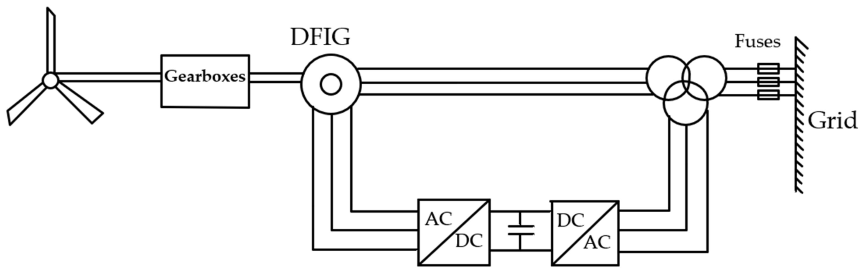
In this paper, a doubly fed induction generator (DFIG) is used as the generating output of a wind turbine. In the local area, electrical energy is generated by the DFIG, and its detailed structure is shown in Figure 1. The simplified mathematical model of the wind turbine model is discussed in the below, and the detailed parameters are given in

Table 1. Parameters of power system.

Parameter	Physical Significance
$f$	Nominal system frequency of the power system
$P_{mech}$	Mechanical power of gas turbine
$P^L$	Sudden load disturbance
$P_v$	Steam valve position
$P_e$	Supplementary control action
$M^a$	Angular momentum
$T_G$	Speed governor time constant
$T_{CH}$	Changing time constant (prime mover)
$P_{ref}$	Reference setpoint
$D$	Equivalent damping coefficient of generator
${\beta }_0$	Frequency bias constant
$y$	System measurement output

. The main source of these equations is [14], and we made appropriate adjustments to the form and dimensionality of some equations.

$${\dot{i}}_{qr}=-\left(\frac{1}{T_1}\right)i_{qr}+\left(\frac{X_2}{T_1}\right)V_{qr}$$

(1)

$$\dot{w_r}=-\left(\frac{X_3}{2H_t}\right)i_{qr}+\left(\frac{1}{2H_t}\right)T_m$$

(2)

$$P_e=w_r{X}_3{i}_{qr}$$

(3)

$$T_e=i_{qs}=-\frac{L_m}{L_s}{i}_{qr}$$

(4)

By linearizing the Taylor series, we can reduce (3) to

$$P_e=w_{opt}{X}_3{i}_{qr}$$

(5)

where $w_{opt}$ is the rotational speed operating point of the wind turbine, $T_e$ is the electric revolution, $T_m$ is the mechanical torque, $i_{qr}$ is the $q$-axis component of the rotor current, $i_{qs}$ is the $q$-axis component of the stator current, $V_{qr}$ is the $q$-axis component of the rotor voltage, $H_t$ is the equivalent inertia constant of the wind turbine, and $w_r$ is the rotational speed of the wind turbine.

$$X_2=\frac{1}{R_r}, X_3=\frac{L_m}{L_s}, T_1=\frac{L_0}{w_s{R}_r}$$

$$L_0=L_r+\frac{L_m^2}{L_S}, L_s=L_{ls}+L_m, L_r=L_{lr}+L_m$$

(6)

where $w_s$ is the synchronous speed of the wind turbine, $L_m$ is the magnetized inductance, $L_{lr}$ is the rotor leakage inductance, $L_{ls}$ is the stator leakage inductance, $L_r$ is the rotor self-inductance, $L_s$ is the stator self-inductance, and $R_r$ is the rotor resistance.

The frequency deviation of the wind power region can be described by the following dynamic equation:

$$\mathrm{\Delta }\dot{f}=-\frac{D}{M^a}\mathrm{\Delta }f+\frac{1}{M^a}\mathrm{\Delta }{P}_m+\frac{1}{2M^a}\mathrm{\Delta }{P}_e-\frac{1}{M^a}\mathrm{\Delta }{P}^L$$

(7)

The turbine dynamic in the wind power region is depicted as

$$\mathrm{\Delta }\dot{P_m}=-\frac{1}{T_{CH}}\mathrm{\Delta }{P}_m+\frac{1}{T_{CH}}\mathrm{\Delta }{P}_v$$

(8)

The governor dynamic of the wind power region can be given as

$$\mathrm{\Delta }\dot{P_v}=-\frac{1}{T_G}\mathrm{\Delta }f-\frac{1}{T_G}\mathrm{\Delta }{P}_v+\frac{1}{T_G}\mathrm{\Delta }{P}_{ref}$$

(9)

The area control error of the region is given as

$$ACE={\beta }_0\mathrm{\Delta }f$$

(10)

According to the above expressions, the frequency response of the system under load disturbance $z=\mathrm{\Delta }{P}^L$ can be described in the form of the following state space equation [14]:

$$\dot{x}=Ax+Bu+Ez$$

(11)

$$y=Cx$$

(12)

$$A=\left[\begin{array}{cccc}-\frac{D}{M^a}& \frac{1}{M^a}& 0& -\frac{X_3{W}_{opt}}{M^a}\\ 0& -\frac{1}{T_{CH}}& \frac{1}{T_{CH}}& 0\\ -\frac{1}{T_G}& 0& -\frac{1}{T_G}& 0\\ 0& 0& 0& -\frac{1}{T_1}\end{array}\right], B=\left[\begin{array}{cc}0& 0\\ 0& 0\\ \frac{1}{T_G}& 0\\ 0& \frac{X_2}{T_1}\end{array}\right]$$

(13)

$$E=\left[\begin{array}{c}-\frac{1}{M^a}\\ 0\\ 0\\ 0\end{array}\right], C=\left[\begin{array}{cccc}{\beta }_0& 0& 0& 0\end{array}\right]$$

(14)

$$x=\left[\begin{array}{c}\mathrm{\Delta }f\\ \mathrm{\Delta }{P}_m\\ \mathrm{\Delta }{P}_v\\ \mathrm{\Delta }{i}_{qr}\end{array}\right], u=\left[\begin{array}{c}\mathrm{\Delta }{P}_{ref}\\ \mathrm{\Delta }{V}_{qr}\end{array}\right]$$

(15)

where x represents the state of the system, u represents the control input, and y represents the output of the system.

3. Frame and Algorithm of Wind Turbine

3.1. Particle Swarm Optimization Analysis

3.1.1. Basic Particle Swarm Optimization Algorithm

Particle swarm optimization is widely used as a classical swarm intelligent optimization algorithm. The algorithm simulates the predation behavior of a flock of birds. Each individual in the flock is regarded as a particle with velocity and position attributes. Each particle searches for the optimal solution of the individual in the search space and shares the optimal solution of the individual with the group to obtain the global optimal solution of the current state. At the same time, each particle also adjusts its flight speed and direction according to the optimal solution information of the population and eventually forms a new population. Compared with other random search algorithms, the PSO algorithm does not have too many adjustable parameters. It is simple and easy to implement and has high precision and fast convergence, which can achieve good application effects in LFC for power system fields [28,29].

In the D-dimensional search space, a population contains N particles, and the position of the $i$th particle is expressed as $X_i$ = ($x_{i1},x_{i2}\dots x_{iD}$) in the D-dimensional space, with velocity $V_i$ = ($v_{i1},v_{i2}\dots v_{iD}$), $i$ = 1, 2, …N. At the same time, the iteration formula is used to update the velocity and position of the particles, and the individual and population optimal values of the next generation of particles are obtained.

$$V_{id}\left(k+1\right)=w{V}_{id}\left(k\right)+c_1{r}_1\left(P_{id}\left(k\right)-X_{id}\left(k\right)\right)+c_2{r}_2(P_{gd}\left(k\right)-X_{id}\left(k\right)$$

(16)

$$X_{id}\left(k+1\right)=X_{id}\left(k\right)+V_{id}\left(k+1\right)$$

(17)

where w is the inertia factor, $r_1$ and $r_2$ are random numbers in [0, 1], $c_1$ and $c_2$ are learning factors, and $P_i$ and $P_g$ are the individual optimal position and the global optimal position of the iteration up to the present.

3.1.2. Improvement in Particle Swarm Optimization Algorithm

The traditional PSO algorithm still has the risk of non-convergence, so this paper adopts an improved strategy for the PSO algorithm, that is, introducing the iterative process of asynchronous learning factors. By improving the learning factors, the global search ability in the early stage is balanced with the local search ability in the late stage. We select larger $c_1$ with smaller $c_2$ in the early stage, enhance the global search ability, and avoid falling into the local optimum. In the later stage, the opposite happens, i.e., we enhance the local search ability and accurately obtain the global optimal solution.

$$c_1\left(t+1\right)=c_{1max}-\left(c_{1max}-c_{1\min }\right)\frac{t}{t_m}$$

(18)

$$c_2\left(t+1\right)=c_{2max}-\left(c_{2max}-c_{2\min }\right)\frac{t}{t_m}$$

(19)

where t is the current iteration number, $t_m$ is the maximum iteration number, $c_{1max}$ and $c_{2max}$ are the maximum learning factors, and $c_{1\min }$ and $c_{2\min }$ are the minimum learning factors.

3.2. Principle and Framework of BP-PI Control Algorithm

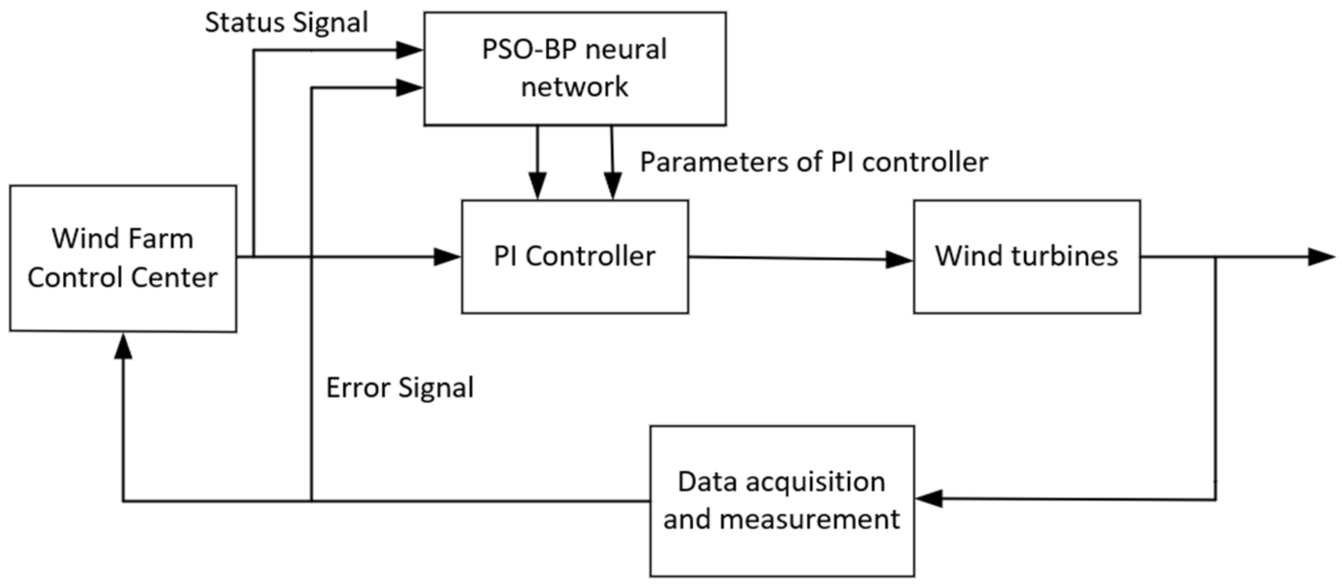
Traditional PI control is one of the most widely used approaches in power industries, and refers to the adjustment of the controlled object by incorporating two fixed parameters through proportion. This paper selects a self-tuning BP-PI controller, which is possible with the participation of an artificial intelligence control algorithm. The controller constantly adjusts the weight of the neural network to achieve the optimal combination of PI gain output by the neural network, which is shown in Figure 2. In the discrete state, the mathematical formulation of PI control is described by

$$u\left(k\right)=K_P\times e\left(k\right)+K_I\times \sum e\left(k\right)$$

(20)

where $K_P$ and $K_I$ are the proportion and integration coefficients and $e\left(k\right)$ represents the deviation of system state input and output at time k.

For LFC with wind turbine participation, since the controller achieves the control effect in the mode of multi-input and multi-output, improved PI control based on the above state space equation is written as

$$u_1\left(k\right)=Q_A\times e\left(k\right)+R_A\times \sum e\left(k\right)$$

(21)

$$u_2\left(k\right)=Q_B\times e\left(k\right)+R_B\times \sum e\left(k\right)$$

(22)

$Q_A$, $Q_B$, $R_A$, and $R_B$ are expressed as

$$\begin{gathered} Q_A=\left[\begin{array}{cccc}{K}_{Pa1}& K_{Pa2}& K_{Pa3}& K_{Pa4}\end{array}\right], Q_B=\left[\begin{array}{cccc}{K}_{Pb1}& K_{Pb2}& K_{Pb3}& K_{Pb4}\end{array}\right], \\ {R}_A=\left[\begin{array}{cccc}{K}_{Ia1}& K_{Ia2}& K_{Ia3}& K_{Ia4}\end{array}\right], R_B=\left[\begin{array}{cccc}{K}_{Ib1}& K_{Ib2}& K_{Ib3}& K_{Ib4}\end{array}\right] \end{gathered}$$

(23)

where $Q_A$ and $Q_B$ represent the proportional coefficient matrices of PI control, $R_A$ and $R_B$ represent the integral coefficient matrices of PI control, $u_1\left(k\right)$ represents the control quantity of valve position deviation quantity $\mathrm{\Delta }{P}_{ref}$ at moment $k$, $u_2\left(k\right)$ represents the control quantity of voltage $\mathrm{\Delta }{V}_{qr}$ at moment $k$, and $e\left(k\right)$ is the deviation of input and output of each state quantity in the system at time $k$.

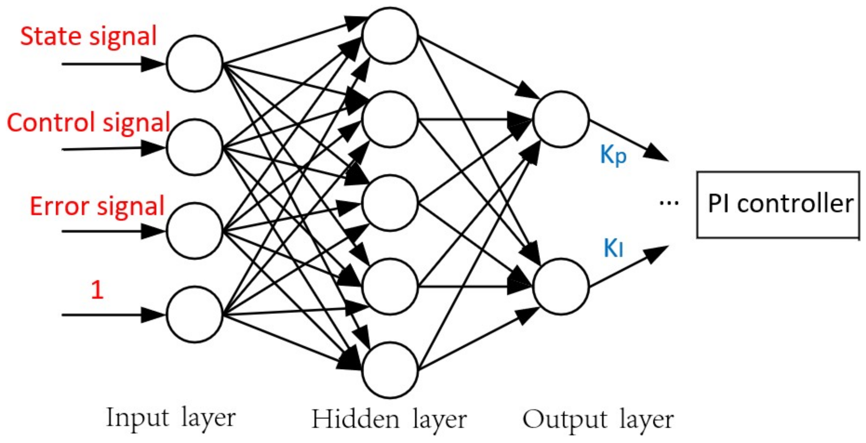
The BP-trained neural network (BPNN) is a multilayer feedforward network trained by an error backpropagation algorithm. Its main characteristics are the forward propagation of signal and the backpropagation of error. Its powerful nonlinear mapping capability enables the BPNN to approximate any nonlinear continuous function with arbitrary precision. At the same time, BPNN has the functions of self-adaptation and self-learning, and the learning content is memorized in the network weight. In addition, the weight of the network is adjusted by means of backpropagation; finally, the network error sum of squares is minimized. In this paper, a three-layer BPNN is used to constantly adjust the weight; finally, the optimal PI parameter matrix combination is obtained. The network structure of the BPNN is shown in Figure 3.

A group of state quantity x and control quantity u, as well as the deviation quantity error and adjustment value 1 of input and output, are selected each time as the input of the BPNN. The structure of the BPNN adopts a 4-5-2 structure. The neural network outputs a group of parameter values of $K_p$ and $K_i$ by learning each time, and a total of 8 groups of values of $K_p$ and $K_i$ are output. The corresponding control effect can be obtained by applying the values of $K_p$ and $K_i$ to the PI controller.

We set the input variable of the BPNN as $x_j$; then, the input–output relationship of the hidden layer can be expressed as

$${net}_i^{\left(2\right)}\left(k\right)={\displaystyle \sum }_{j=1}^M{w}_{ij}^{\left(2\right)}\left(k\right)x_j^{\left(1\right)}$$

(24)

$$O_i^{\left(2\right)}\left(k\right)=f_1\left(ne{t}_i^{\left(2\right)}\left(k\right)-{\theta }_i\right)$$

(25)

where ${net}_i^{\left(2\right)}\left(k\right)$ denotes the node input of the hidden layer of the neural network, ${\theta }_i$ is the threshold value of the neuron of the hidden layer, $w_{ij}^{\left(2\right)}\left(k\right)$ signifies the weight of the neuron of the input layer and the neuron of the hidden layer, and $O_i^{\left(2\right)}\left(k\right)$ is the node output of the hidden layer. The excitation function of the hidden layer is

$$f_1\left(x\right)=\frac{e^x-e^{-x}}{e^x+e^{-x}}$$

(26)

The relationship of the output layer of the BPNN is given by

$${net}_l^{\left(3\right)}\left(k\right)={\displaystyle \sum }_{j=1}^P{w}_{li}^{\left(3\right)}\left(k\right)O_i^{\left(2\right)}\left(k\right)$$

(27)

$$O_l^{\left(3\right)}\left(k\right)=f_2\left(ne{t}_l^{\left(3\right)}\left(k\right)-{\theta }_l\right)$$

(28)

where $w_{li}^{\left(3\right)}\left(k\right)$ is the weight of the hidden layer neuron and the output layer neuron, ${\theta }_l$ is the threshold value of the output layer neuron, and $O_l^{\left(3\right)}\left(k\right)$ represents the output of the output layer. The excitation function of the output layer selects the non-negative sigmoid function, whose expression form is

$$f_2\left(ne{t}_l^{\left(3\right)}\left(k\right)\right)=\frac{e^x}{e^x+e^{-x}}$$

(29)

In the BP neural network backpropagation process, we adjust the connection weights by setting the backpropagation of the error function. The difference between the actual measured output state quantity and the expected output state quantity of the control system is defined as the calculation error of backpropagation, and the performance index function is obtained as follows:

$$e\left(k\right)=yout\left(k\right)-rin\left(k\right)$$

$$E\left(k\right)=\frac{1}{2}{e}^2\left(k\right)$$

(30)

The BP neural network usually adopts the gradient descent method to modify neural network parameters, that is, to adjust connection weights according to the direction of the negative gradient change of performance index function $E\left(k\right)$. The momentum term is introduced in the backpropagation process, and a value proportional to the previous weight change is added to each weight change. The weight updating processes of the output layer and the hidden layer can be described as

$$\mathrm{\Delta }{w}_{li}^{\left(3\right)}\left(k+1\right)=-\beta \frac{\partial E\left(k\right)}{\partial w_{li}^{\left(3\right)}\left(k\right)}+\alpha \mathrm{\Delta }{w}_{li}^{\left(3\right)}\left(k\right)$$

(31)

$$\mathrm{\Delta }{w}_{ij}^{\left(2\right)}\left(k+1\right)=-\beta \frac{\partial E\left(k\right)}{\partial w_{ij}^{\left(2\right)}\left(k\right)}+\alpha \mathrm{\Delta }{w}_{ij}^{\left(2\right)}\left(k\right)$$

(32)

where $\mathrm{\Delta }{w}_{li}^{\left(3\right)}\left(k+1\right)$ and $\mathrm{\Delta }{w}_{ij}^{\left(2\right)}\left(k+1\right)$ represent the weight increments of output layer and hidden layer at moment k + 1, $\mathrm{\Delta }{w}_{li}^{\left(3\right)}\left(k\right)$ and $\mathrm{\Delta }{w}_{ij}^{\left(2\right)}\left(k\right)$ stand for the weight increments of output layer and hidden layer at moment k + 1, β is the learning rate (in the range of $0~1$), and α is the momentum factor (in the range of $0~1$).

The process of signal forward transmission and error backpropagation of the BPNN is the training process of the network. This process makes the actual output of the network gradually approximate to the expected output by adjusting the connection weights of the hidden layer and the output layer inside the network. In general, the typical BPNN needs to be trained on multiple sets of data to achieve the desired effect.

3.3. Specific Implementation Process of IPSO-BPNN-PI-Based Secondary Frequency Control

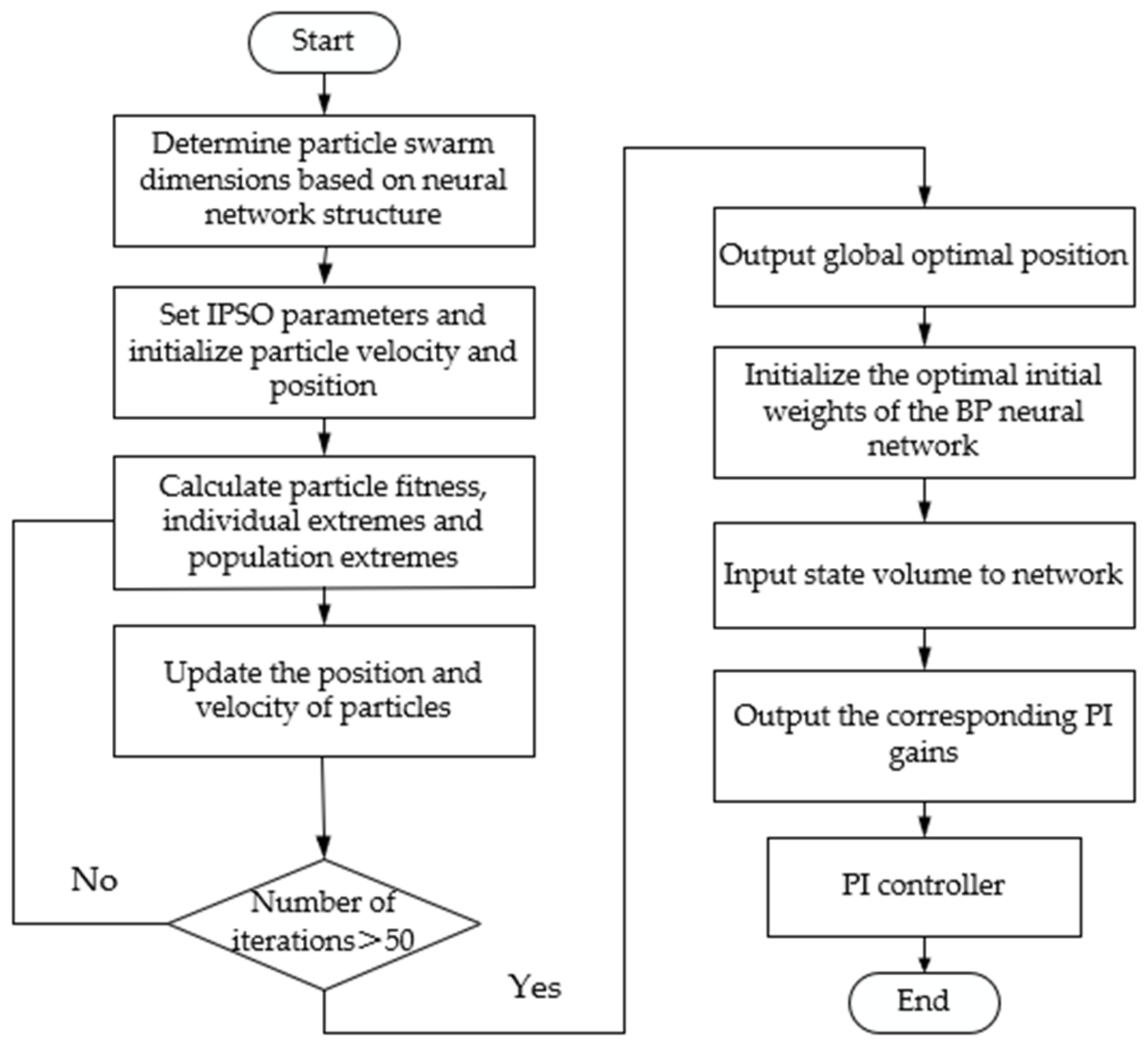
We use the IPSO-BP-PI control strategy to achieve effective control in LFC, as shown in Figure 4. The specific implementation process of IPSO-BPNN-PI-based LFC can be divided into the following 6 steps.

Step 1: The dimension of the particle swarm is determined; the velocity and position of particles are initialized; and learning factors $c_1$ and $c_2$, as well as initial individual optimal value $P_{0best}$ and global optimal value $G_{0best}$, and other related parameters are set.

Step 2: The adaptation value after particle position update and the following fitness function are calculated:

$$fitness=\frac{1}{n}{{\displaystyle \sum }}_{k=1}^n{e}^2\left(k\right)$$

(33)

Step 3: The above improved PSO is adopted to iteratively update the individual optimal value and global optimal value of the particle, and the fitness of the new particle is compared with the fitness of the previous particle. If the number of iterations reaches the maximum set number of iterations, the iteration is ended, and the current optimal solution is output.

Step 4: The optimal solution of the PSO algorithm is used to initialize the optimal initial weight of the BPNN. Then, the network obtains the optimal PI controller parameter combination through the process of signal forward transmission and error reverse transmission.

Step 5: The adjustable parameters of the neural network output are used to adapt the gains of the PI controller in order to reach valve position $\mathrm{\Delta }{P}_{ref}$ and the voltage adjustment of $\mathrm{\Delta }{V}_{qr}$.

Step 6: Control quantities $\mathrm{\Delta }{P}_{ref}$ and $\mathrm{\Delta }{V}_{qr}$ jointly act on the wind turbine and finally achieve the control of the load frequency output of the power system.

4. Simulation and Discussion

An LFC system involving a wind turbine in a certain region was set up. We here set the base simulation sampling interval to 0.3 s. Assuming that there is no power flow switching between the regions, the actual nominal parameters used in the power system simulation are shown below in

Table 2. Model parameters of power system.

$D=2.75 \mathrm{pu}/\mathrm{Hz}$	$w_{opt}=1.18 \mathrm{rad}/\mathrm{s}$
$M^a=3.15 \mathrm{N}·\mathrm{m}$	$R_r=0.00552 \mathrm{pu}$
$T_{CH}=8.0$	$R_s=0.00491 \mathrm{pu}$
$T_G=12.5$	$L_m=3.62 \mathrm{H}$
${\beta }_0=1$	$L_r=0.17 \mathrm{H}$

[7,14].

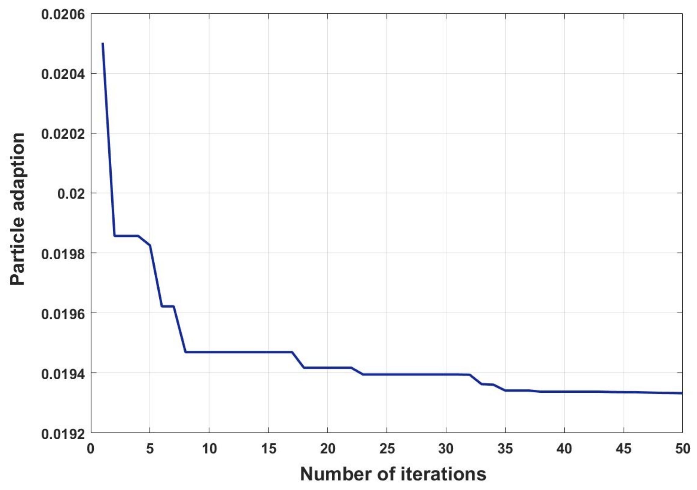
The number of iterations of the control system was set to 50. After 50 iterations, the fitness changes of the optimal individuals of the particle swarm are shown in Figure 5. After 50 iterations, the fitness of the particle swarm tends to be stable, and changes are no longer observed.

• Case study one: Frequency adjustment in the presence of initial frequency errors

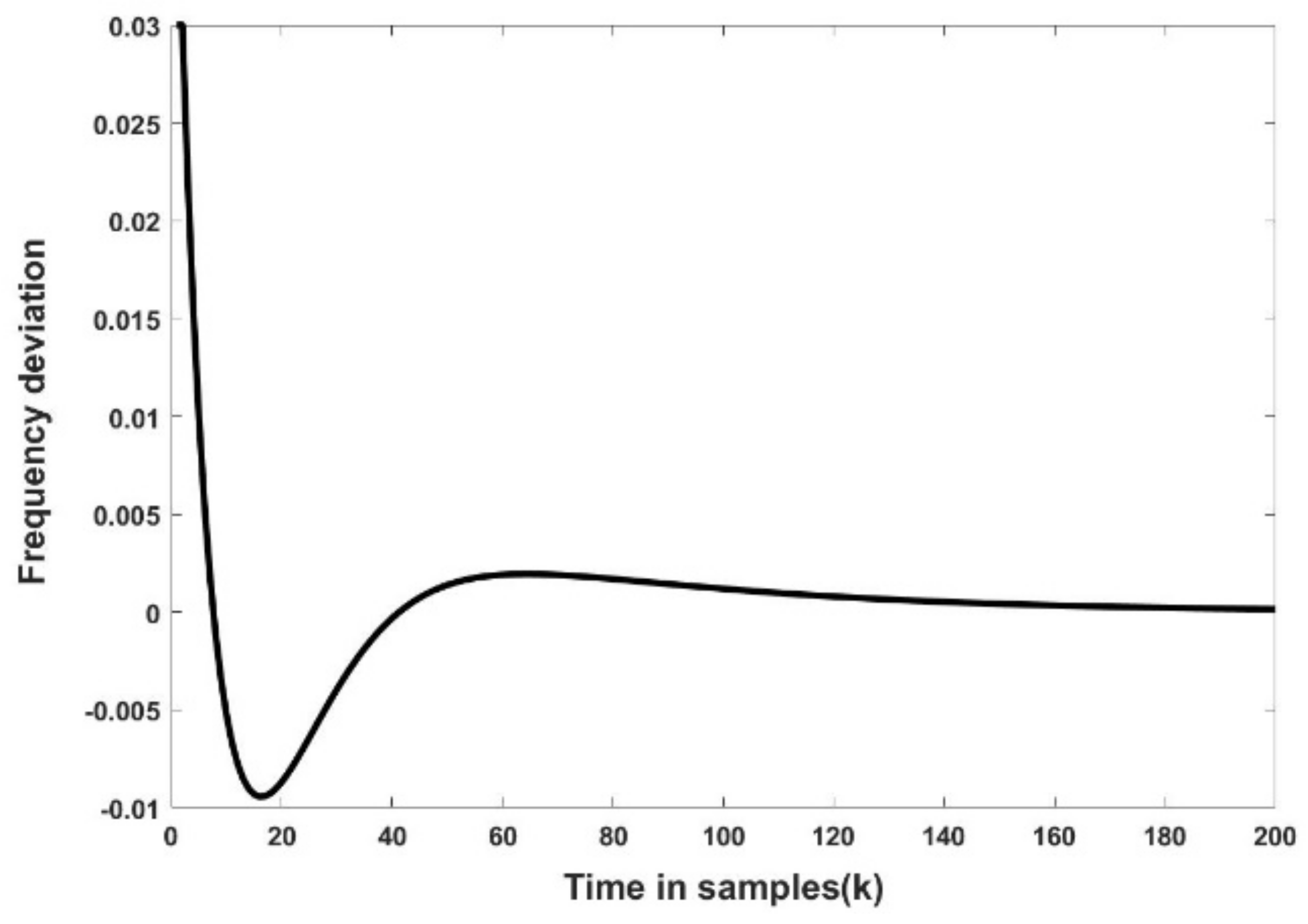
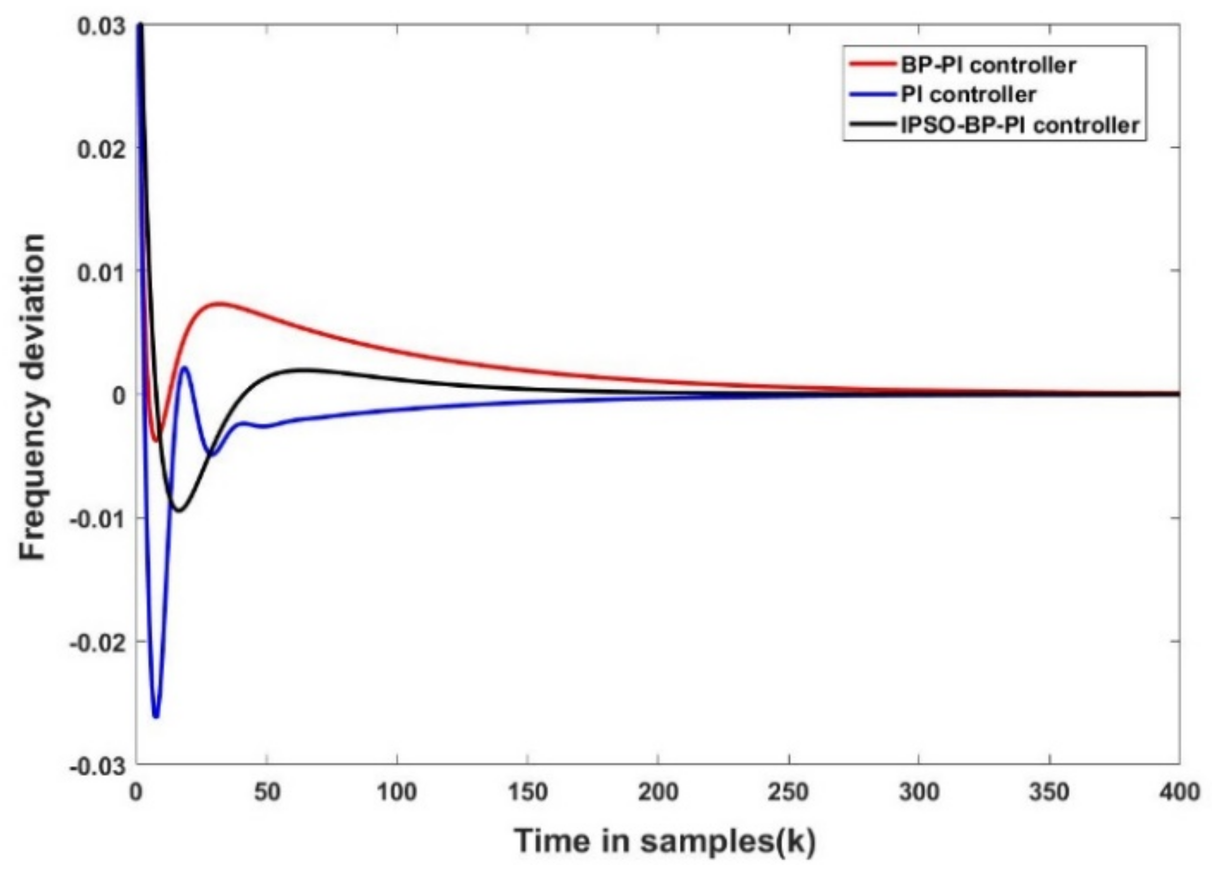
In order to verify the dynamic performance of the system, a simulation test was carried out with an IPSO-BP-PI controller, and the results were evaluated within 60 s to obtain the effect of the change in the frequency deviation of the system output. Meanwhile, we compared this control strategy with conventional PI control and BP-PI control, whose results show that the IPSO-BP-PI control strategy had the best adjustment effect. In the simulation, we set the initial frequency error to 0.03 Hz; the dynamic response curves of the frequency deviation are shown in Figure 6 and Figure 7.

• Case study two: Adjustment process with application of random load disturbance

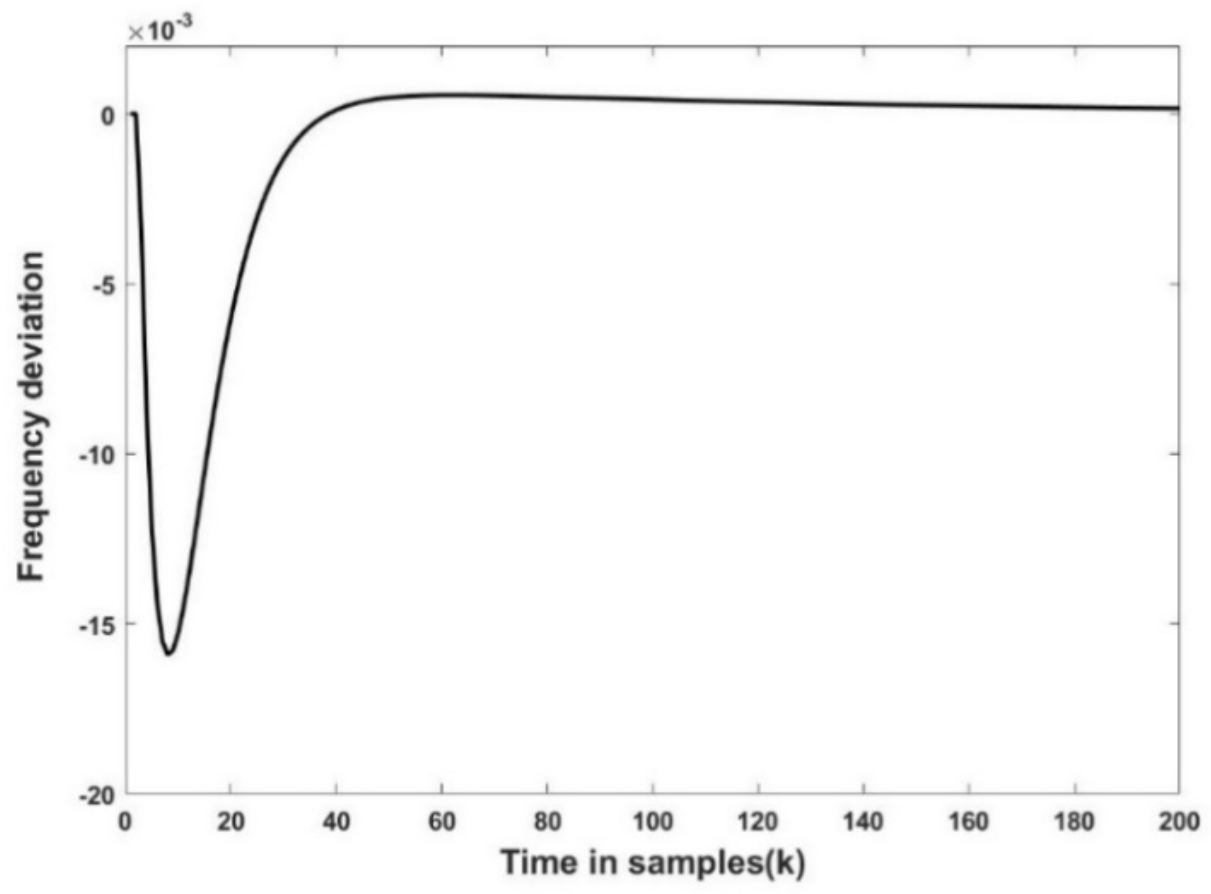
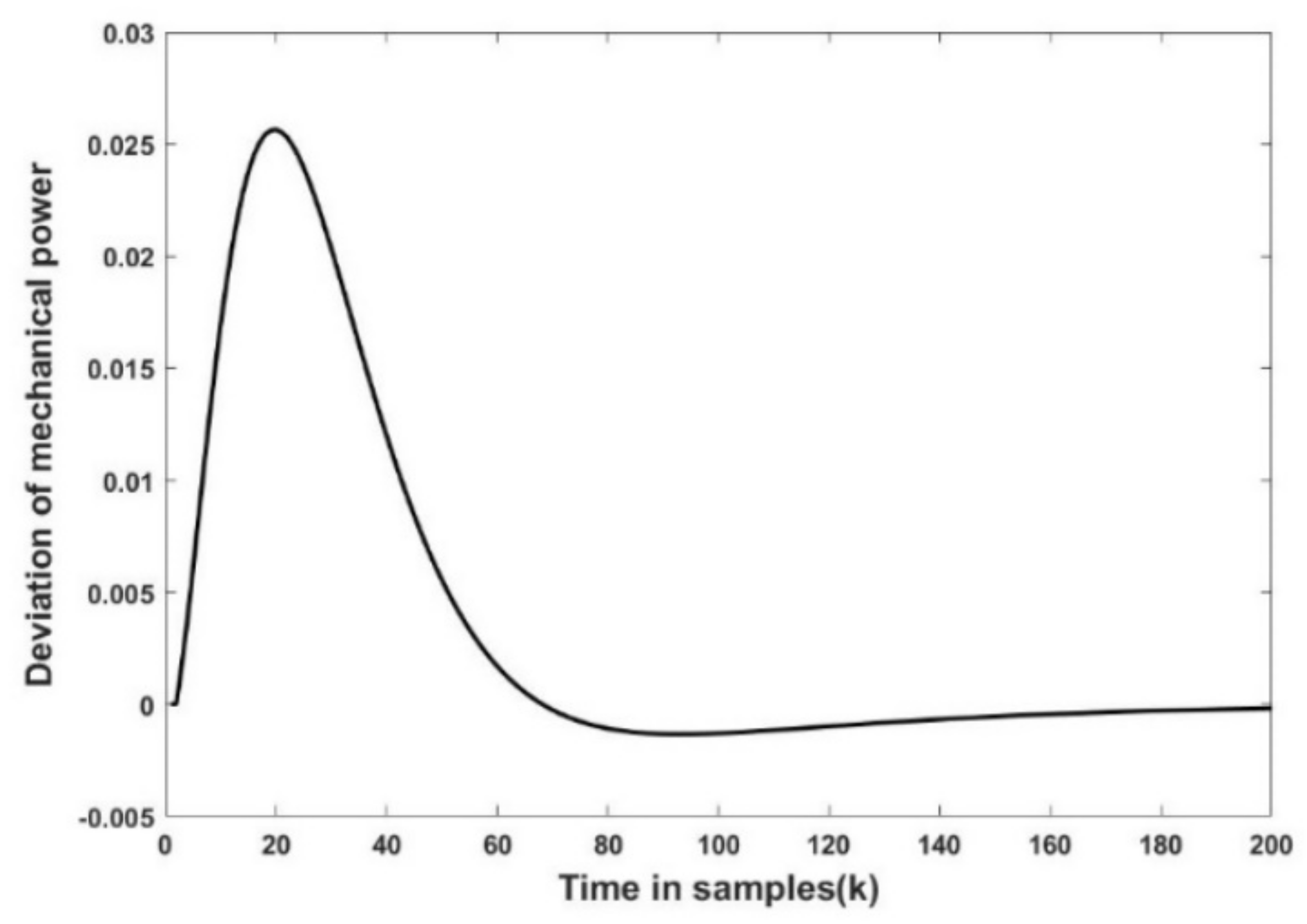
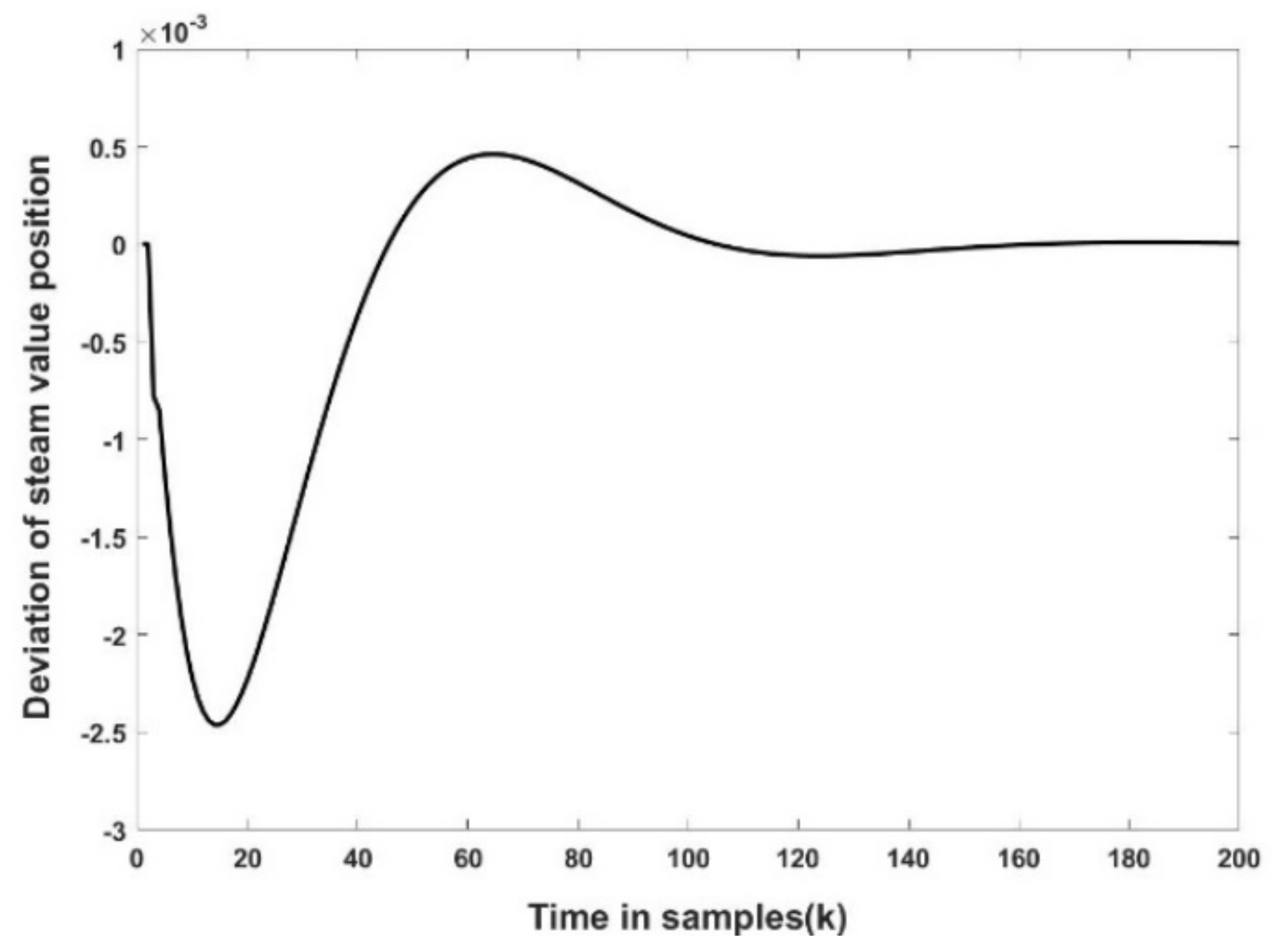
Figure 8, Figure 9 and Figure 10 show the control effects of $\mathrm{\Delta }f,$ $\mathrm{\Delta }{P}_m$, and $\mathrm{\Delta }{P}_v$, respectively, following the application of random disturbance $\mathrm{\Delta }{P}^L$ at the initial moment. On the whole, the frequency deviation, the variation range of mechanical power deviation, and the governor output power deviation were relatively stable from a numerical point of view, and all converged to 0 within a short period of time after a period of fluctuation. Furthermore, to verify the proposed scheme, we used MATLAB to test the maximum overshoot, minimum overshoot, adjustment time, and the magnitude of the stability error, which are given in

Table 3. Specific values for random load demand.

Parameter	Max. Value	Min. Value	Stable Time	Stable Error
$\mathrm{\Delta }f$	0.00086	−0.01596	15.81	−0.00024
$\mathrm{\Delta }{P}_m$	0.02611	−0.00137	33.48	0.00012
$\mathrm{\Delta }{P}_v$	0.00047	−0.00248	37.02	0.00007

. The measurements validated the effectiveness of the IPSO-BP-PI control method.

• Case study three: Frequency tuning with perturbations applied at subsequent intervals

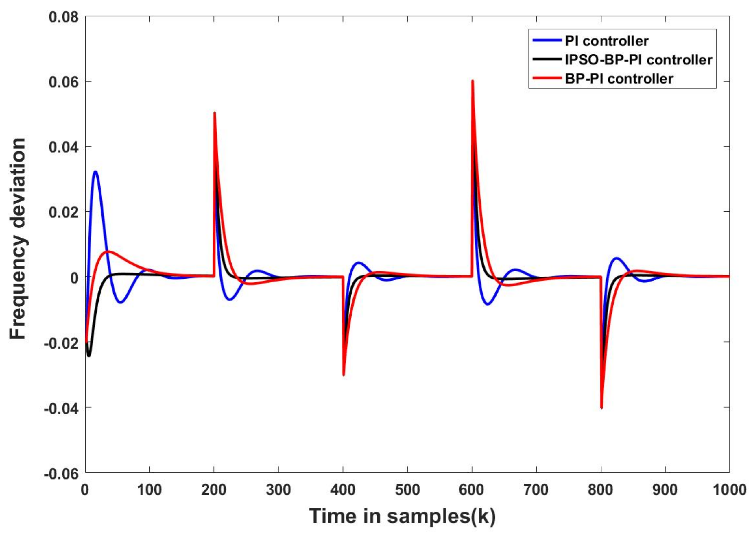
Here, we simulated the frequency adjustment more realistically using the IPSO-BP-PI controller when the actual area is subjected to load disturbance. Power systems are always subjected to varying degrees of load demand changes during real-time operation. To clearly demonstrate the frequency tuning capability of the IPSO-BP-PI controller, we simulated the frequency response when random perturbations $\mathrm{\Delta }{P}_L=0.1\times \left(rand\left(1\right)-0.5\right)$ were applied every other 60 s. The frequency response effects with PI control, BP-PI control, and IPSO-BP-PI control strategies were respectively compared. The frequency responses in these cases using different techniques are shown in Figure 11. With the participation of the doubly fed wind turbine, the three controllers all converged to zero and had a certain effect on LFC, ignoring the information exchange between the region and the outside region. In comparison, the IPSO-BP-PI controller showed shorter stabilizing time and smaller overshoot, which is ideal for regulating different load changes. Meanwhile, the method effectively improved the frequency response of the system and avoided redundant oscillation links, as clearly shown in

Table 4. Stable time of the system.

	Stable Time 1	Stable Time 2	Stable Time 3	Stable Time 4	Stable Time 5
PI	46.86	30.39	28.47	38.25	35.17
BP-PI	36.57	25.72	23.62	33.51	31.64
IPSO-BP-PI	15.85	10.67	9.91	11.76	10.26

. The superior effect of the IPSO-BP-PI controller on the LFC of local random disturbance was also verified.

5. Conclusions

The requirements of grid-connected wind power rules around the world make it easy to conclude that system frequency regulation involving wind power will likely become an inevitable requirement for future new energy development [30,31]. In this paper, an IPSO-BP-PI frequency control method for wind power systems is proposed to solve the problems of large load disturbance and high uncertainty in wind power systems. The improved PSO algorithm is used to optimize the initial weight of the BPNN, which reduces and stabilizes particle fitness around 0.194 and increases the stability of the neural network. Using the adaptive ability of the optimized BPNN to adjust the gain parameters of the PI controller in real time overcomes the problem of the traditional PI controller used in time-varying systems. The optimization scheme was applied to regional LFC involving wind turbines. The simulation test results show that the IPSO-BP-PI control strategy had better instantaneous response effect, which effectively reduced the stable error of the frequency to less than ${10}^{-3}$. Additionally, the IPSO-BP-PI control approach improves the accuracy and significantly shortens adjustment times for frequency stabilization, which has a remarkable effect on solving the load disturbance caused by uncertain factors compared with traditional PI control and BP-PI control. In the future, we aim to investigate LFC for power systems with the integration of multiple renewable energy resources in the presence of unforeseen disturbances.

References

- Sadorsky, P. Wind energy for sustainable development: Driving factors and future outlook. J. Clean. Prod. 2021, 289, 125779. [Google Scholar] [CrossRef]
- Veerasamy, V.; Wahab, N.I.A.; Ramachandran, R.; Othman, M.L.; Hizam, H.; Irudayaraj, A.X.R.; Guerrero, J.M.; Kumar, J.S. A Hankel Matrix Based Reduced Order Model for Stability Analysis of Hybrid Power System Using PSO-GSA Optimized Cascade PI-PD Controller for Automatic Load Frequency Control. IEEE Access 2020, 8, 71422–71446. [Google Scholar] [CrossRef]
- Liu, F.; Ma, J. Equivalent input disturbance-based robust LFC strategy for power system with wind farms. IET Gener. Transm. Distrib. 2018, 12, 4582–4588. [Google Scholar] [CrossRef]
- Mohseni, N.; Bayati, N. Robust Multi-Objective H2/H∞ Load Frequency Control of Multi-Area Interconnected Power Systems Using TS Fuzzy Modeling by Considering Delay and Uncertainty. Energies 2022, 15, 5525. [Google Scholar] [CrossRef]
- Debnath, M. Whale Optimization Algorithm Tuned Fuzzy Integrated PI Controller for LFC Problem in Thermal-hydro-wind Interconnected System. In Applications of Computing, Automation and Wireless Systems in Electrical Engineering: Proceedings of MARC 2018; Springer: Singapore, 2019; pp. 67–77. [Google Scholar]
- Payal, R.; Kumar, D. Load Frequency Control of Wind Integrated Power System Using Intelligent Control Techniques. Int. J. Adv. Eng. Manag. (IJAEM) 2021, 3, 1339–1353. [Google Scholar]
- Fan, W.; Hu, Z.; Veerasamy, V. PSO-Based Model Predictive Control for Load Frequency Regulation with Wind Turbines. Energies 2022, 15, 8219. [Google Scholar] [CrossRef]
- Abhayadev, S.; Kumar, P.R. Effect of DFIG Wind Turbines on LFC in a Sliding Mode Controlled Power System. In Proceedings of the 6th International Conference for Convergence in Technology (I2CT), Maharashtra, India, 2–4 April 2021; pp. 1–6. [Google Scholar] [CrossRef]
- Abazari, A.; Monsef, H.; Wu, B. Load frequency control by de-loaded wind farm using the optimal fuzzy-based PID droop controller. IET Renew. Power Gener. 2018, 13, 180–190. [Google Scholar] [CrossRef]
- Yan, Z.; Xu, Y. Data-Driven Load Frequency Control for Stochastic Power Systems: A Deep Reinforcement Learning Method with Continuous Action Search. IEEE Trans. Power Syst. 2018, 34, 1653–1656. [Google Scholar] [CrossRef]
- Xu, Z.; Wang, D.; Yi, G.; Hu, Z. Asynchronous Tracking Control of Amplitude Signals in Vibratory Gyroscopes with Partially Unknown Mode Information. IEEE Trans. Ind. Electron. 2022, 1–10. [Google Scholar] [CrossRef]
- Hu, Z.; Liu, S.; Luo, W.; Wu, L. Intrusion-Detector-Dependent Distributed Economic Model Predictive Control for Load Frequency Regulation with PEVs Under Cyber Attacks. IEEE Trans. Circuits Syst. I Regul. Pap. 2021, 68, 3857–3868. [Google Scholar] [CrossRef]
- Hu, Z.; Liu, S.; Wu, L. Credibility-based distributed frequency estimation for plug-in electric vehicles participating in load frequency control. Int. J. Electr. Power Energy Syst. 2021, 130, 106997. [Google Scholar] [CrossRef]
- Ma, M.; Liu, X.; Zhang, C. LFC for multi-area interconnected power system concerning wind turbines based on DMPC. IET Gener. Transm. Distrib. 2017, 11, 2689–2696. [Google Scholar] [CrossRef]
- Zhang, K.; Zhou, B.; Duan, G. Event-Triggered and Self-Triggered Control of Discrete-Time Systems with Input Constraints. IEEE Trans. Syst. Man Cybern. Syst. 2020, 52, 1948–1957. [Google Scholar] [CrossRef]
- Mohamed, T.H.; Alamin, M.A.M.; Hassan, A.M. A novel adaptive load frequency control in single and interconnected power systems. Ain Shams Eng. J. 2020, 12, 1763–1773. [Google Scholar] [CrossRef]
- Navarrete, E.C.; Trejo Perea, M.; Jáuregui Correa, J.C.; Carrillo Serrano, R.V.; Moreno, G.J.R. Expert Control Systems Implemented in a Pitch Control of Wind Turbine: A Review. IEEE Access 2019, 7, 13241–13259. [Google Scholar] [CrossRef]
- Yu, T.; Liu, J.; Zeng, Y.; Zhang, X.; Zeng, Q.; Wu, L. Stability Analysis of Genetic Regulatory Networks with Switching Parameters and Time Delays. IEEE Trans. Neural Netw. Learn. Syst. 2017, 29, 3047–3058. [Google Scholar] [CrossRef] [PubMed]
- Prasad, S.; Ansari, M.R. Frequency regulation using neural network observer based controller in power system. Control Eng. Pract. 2020, 102, 104571. [Google Scholar] [CrossRef]
- Yu, T.; Zhang, X.; Wang, X. Global Exponential Stability Analysis for A Class of Coupled Cyclic Genetic Regulatory Networks with Multiple Time-Varying Delays. IFAC-PapersOnLine 2021, 54, 23–28. [Google Scholar] [CrossRef]
- Wang, Y.; Wang, T.; Yang, X.; Yang, J. Gradient Descent-Barzilai Borwein-Based Neural Network Tracking Control for Non-linear Systems with Unknown Dynamics. IEEE Trans. Neural Netw. Learn. Syst. 2023, 34, 305–315. [Google Scholar] [CrossRef] [PubMed]
- Hu, Z.; Liu, S.; Luo, W.; Wu, L. Resilient Distributed Fuzzy Load Frequency Regulation for Power Systems Under Cross-Layer Random Denial-of-Service Attacks. IEEE Trans. Cybern. 2020, 52, 2396–2406. [Google Scholar] [CrossRef] [PubMed]
- Sahu, P.C.; Mishra, S.; Prusty, R.C.; Panda, S. Improved-salp swarm optimized type-II fuzzy controller in load frequency control of multi area islanded AC microgrid. Sustain. Energy Grids Netw. 2018, 16, 380–392. [Google Scholar] [CrossRef]
- Rahman, J.; Tafticht, T.; Doumbia, M.; Mutombo, N. Dynamic Stability of Wind Power Flow and Network Frequency for a High Penetration Wind-Based Energy Storage System Using Fuzzy Logic Controller. Energies 2021, 14, 4111. [Google Scholar] [CrossRef]
- Mokhtar, M.; Marei, M.I.; Sameh, M.A.; Attia, M.A. An Adaptive Load Frequency Control for Power Systems with Renewable Energy Sources. Energies 2022, 15, 573. [Google Scholar] [CrossRef]
- Li, J.; Cheng, J.-H.; Shi, J.-Y.; Huang, F. Brief Introduction of Back Propagation (BP) Neural Network Algorithm and its Improvement. In Advances in Computer Science and Information Engineering; Springer: Berlin/Heidelberg, Germany, 2012; pp. 553–558. [Google Scholar] [CrossRef]
- Veerasamy, V.; Wahab, N.I.A.; Ramachandran, R.; Othman, M.L.; Hizam, H.; Kumar, J.S.; Irudayaraj, A.X.R. Design of single- and multi-loop self-adaptive PID controller using heuristic based recurrent neural network for ALFC of hybrid power system. Expert Syst. Appl. 2021, 192, 116402. [Google Scholar] [CrossRef]
- Panda, D.K.; Das, S.; Townley, S. Toward a More Renewable Energy-Based LFC Under Random Packet Transmissions and Delays with Stochastic Generation and Demand. IEEE Trans. Autom. Sci. Eng. 2020, 19, 1217–1232. [Google Scholar] [CrossRef]
- Shouran, M.; Anayi, F.; Packianather, M.; Habil, M. Different Fuzzy Control Configurations Tuned by the Bees Algorithm for LFC of Two-Area Power System. Energies 2022, 15, 657. [Google Scholar] [CrossRef]
- Luo, W.; Wang, F.; Li, Q.J.; Xie, H. Research on Development of Wind Power Grid Integration in China. Adv. Mater. Res. 2012, 608-609, 560–563. [Google Scholar] [CrossRef]
- Holjevac, N.; Zidar, M.; Krpan, M.; Kuzle, I. Optimizing the Grid Connection Scheme of the Wind Power Plant. In Proceedings of the 14th Conference on Sustainable Development of Energy, Water and Environment Systems (SDEWES), Dubrovnik, Croatia, 1–6 October 2019. [Google Scholar]
Figure 1.
Structure of a doubly fed wind turbine.
Figure 2.
IPSO-BP-PI controller of the power system.
Figure 3.
Structure of BP neural network.
Figure 4.
IPSO algorithm for optimizing neural network process.
Figure 5.
Convergence curve of IPSO.
Figure 6.
Dynamic response of frequency using IPSO-BP-PI strategy with DFIG-based wind turbine.
Figure 7.
Dynamic responses of frequency using three strategies with DFIG-based wind turbine.
Figure 8.
Frequency dynamic curve in the presence of load disturbance using IPSO-BP-PI technique.
Figure 9.
Dynamic response of mechanical power using IPSO-BP-PI technique.
Figure 10.
Dynamic response of steam value position using IPSO-BP-PI technique.
Figure 11.
Frequency regulation curves with random perturbation using three techniques.