
Investigation of Data Pre-Processing Algorithms for Power Curve Modeling of Wind Turbines Based on ECC
School of Mechanical Engineering, Hunan University of Science and Technology, Xiangtan 411201, China
*
Author to whom correspondence should be addressed.
Energies 2023, 16(6), 2679; https://0-doi-org.brum.beds.ac.uk/10.3390/en16062679
Submission received: 16 February 2023
/
Revised: 10 March 2023
/
Accepted: 10 March 2023
/
Published: 13 March 2023
(This article belongs to the Special Issue Recent Advances in Marine and Offshore Renewable Power Generation Technologies)
Abstract
:Data pre-processing is the first step of using SCADA data to study the performance of wind turbines. However, there is a lack of knowledge of how to obtain more effective data pre-processing algorithms. This paper fully explores multiple data pre-processing algorithms for power curve modeling. A three-stage data processing mode is proposed, namely, preliminary data filtering and compensation (Stage I), secondary data filtering (Stage II), and single-valued processing (Stage Ⅲ). Different data processing algorithms are selected at different stages and are finally merged into nine data processing algorithms. A novel evaluation method based on energy characteristic consistency (ECC) is proposed to evaluate the reliability of various algorithms. The influence of sliding mode and benchmark of Binning on data processing has been fully investigated through indicators. Four wind turbines are selected to verify the advantages and disadvantages of the nine data processing methods. The result shows that at the same wind speed, the rotational speed and power values obtained by MLE (maximum likelihood estimation) are relatively high among the three single-valued methods. Among the three outlier filtering methods, the power value obtained by KDE (kernel density estimation) is relatively large. In general, KDE-LSM (least square method) has good performance in general. The sum of four evaluating index values obtained by KDE-LSM from four wind turbines is the smallest.
1. Introduction
Renewable energy, such as wind energy, is becoming more and more popular because it is cleaner and more efficient than traditional energy [1,2,3]. Wind turbines are the core equipment that captures wind energy and converts it into electricity. For a long time, the design and optimization of wind turbines have been the focus of the wind power industry [4,5]. Many new methods and advanced tools have been used in the design and analysis of wind turbines, such as the CFD method, which is also widely used in various blade designs [6,7,8]. To meet the need for more wind farms, Tang, X. et al. carried out theoretical and experimental research on low wind speed wind turbines and the power output is significantly improved through blade optimization [9]. At present, the single-unit capacity of wind turbines is becoming larger and larger, and many wind turbines with a diameter of more than 100 m now exist. Even wind turbines more than 200 m in diameter have been designed. Because large wind turbines are assembled and debugged on-site, the actual performance can only be accurately obtained after operation. Due to the harsh working environment of wind turbines, the safety and operating costs of wind turbines have always been sensitive issues. Understanding the actual performance of wind turbines is of great help to improve their design and maintenance capabilities [10,11,12]. In this scenario, the use of SCADA (supervisory control and data acquisition) data is widely carried out [13,14,15]. With the extension of service time, the data stored in the SCADA system is accumulated year-by-year, which not only reflects the current operation status of wind turbines but also stores their historical service status. Therefore, making full use of SCADA data information during service is an important way to deepen our understanding and optimize the control strategy.
In recent years, much research on the operation mechanism and maintenance of wind turbines has been carried out based on SCADA data [16,17,18]. Moreover, the research based on SCADA data is continuing with a more vigorous trend. For example, Singh, U. et al. developed a prediction tool based on time series data to estimate wind power using SCADA data [19]. Morshedizadeh, M. et al. carried out a case study on rotor overspeed fault diagnosis of wind turbines based on SCADA data, vibration analysis, and field detection [20]. Astolfi, D. et al. used SCADA data to discuss the long-term performance evaluation of wind turbines [21]. Based on SCADA data, Dong, X. et al. built the blade icing identification model of wind turbines [22]. However, because of random factors in the external environment, the equipment itself, and the connected power grid, SCADA data contains random interference information, which leads to its inability to be directly used for performance evaluation and analysis. Researchers have proposed a variety of SCADA data pre-processing methods, including data filtering, averaging, single-valued processing based on kernel density, etc. [23,24]. Yang, W. et al. used the averaging method to pre-process the data after filtering the outliers of the original SCADA data and evaluated the operation status of wind turbines [25]. According to the type of abnormal data of wind turbines, Yao, Q. et al. proposed a new combination method to clean up the anomalous SCADA data. In the proposed combination method, a pre-processing method for removing outliers of the power curve based on the operation mechanism is first proposed, and a new data cleaning method, TTLOF, is presented, which quantifies specific data points and eliminates outliers by setting parameter thresholds [24]. Marti-Puig, P. et al. evaluated the impact of using several widely used technologies (such as Quantile, Hampel, and ESD) to remove extreme values with recommended cut-off values [26]. Long, H. et al. transformed the problem of wind turbine data cleaning into the problem of image processing, and a three-dimensional (3D) WPC image was constructed [27]. Wang, Y. et al. designed a combined wind speed prediction system based on two-stage data pre-processing and multi-objective optimization. The main function of two-stage data pre-processing is to decompose and reshape the raw data to reduce noise and chaos disturbance [28]. To use SCADA data for power curve cleaning, Morrison, R. et al. compared three data pre-processing algorithms [29].
It has become a consensus that data pre-processing is very important in the process of using wind turbine SCADA data [26,30]. Despite the previous studies, there are still some issues to be further studied on how to effectively and reliably conduct SCADA data pre-processing. For example, there are several data pre-processing algorithms, but what are the differences between them? This problem lacks comprehensive and systematic research. In addition, the fundamental purpose of data pre-processing for SCADA data is to provide the reliability of data analysis, but how can the reliability of the data pre-processing itself be ensured? In our previous study, three evaluation indexes for the pre-processing algorithm are presented, including (1) the consistency of physical characteristics; (2) the robustness of the sampling time; (3) the robustness of the sampling frequency [31]. In this paper, a novel evaluation method based on the energy characteristic consistency (ECC) of wind turbines is proposed to evaluate the reliability of various data pre-processing algorithms. A three-stage data processing mode is proposed, namely, preliminary data filtering and compensation (Stage Ⅰ), secondary data filtering (Stage Ⅱ), and single-valued processing (Stage Ⅲ). Its main purpose is to improve the reliability of data pre-processing. Different data processing algorithms are selected at different stages and finally merged into nine data processing algorithms. Moreover, the nine data processing algorithms are compared and analyzed from different perspectives. The main contribution of this paper is to make a comprehensive comparison of the SCADA data of wind turbines, to gain a deeper understanding and provide a basis for practical application.
In general, the innovative contributions of the paper can be summarized as follows.
- A three-stage data processing mode for power curve modeling of wind turbines is proposed.
- A novel evaluation method based on the energy characteristic consistency (ECC) of wind turbines is proposed.
- The advantages and disadvantages of the nine data processing methods are verified by four wind turbines.
The remainder of the paper is organized as follows. In Section 2, energy characteristic consistency (ECC) is introduced and defined. Three performance curves of wind turbines are projected into three planes in a three-dimensional coordinate system, respectively. In Section 3, the data relationship for power curve modeling is established. The reason why the wind speed measured by the nacelle anemometer needs to be compensated is theoretically proved. A three-stage data processing mode for the power curve modeling of wind turbines is presented in Section 4. This section also explains why preliminary data filtering and compensation, secondary data filtering based on Binning, and single-valued processing based on Binnig are needed. In Section 5, the influence of sliding mode and benchmark of Binning on data processing has been fully investigated through four quantitative indicators. Four wind turbines are selected to verify the advantages and disadvantages of data processing methods. Finally, Section 6 ends the paper by summarizing the main achievements.
2. Energy Characteristic Consistency (ECC)
Wind turbines are complex devices that convert air kinetic energy into mechanical energy and then into electrical energy. With the increasing diameter of wind turbines, the cost is growing higher and higher. Performance is also expected to be better and more stable. In the design and operation of wind turbines, the behavior characteristics of capturing aerodynamic energy are of great concern. There are three curves commonly used to describe this energy feature: the curve of wind speed–power, the curve of wind speed–rotational speed, and the curve of rotational speed–power. The relationship between wind speed and power is generally expressed as
where, P (W) is power, is power coefficient, () is air density, S () is the area swept by the wind rotor, and v (m/s) is wind speed.
In Equation (1), wind speed and power coefficient are variables. Wind speed is the description of airflow velocity in nature, which has the characteristics of time-variation and randomness. The power coefficient is the key parameter to reflect the wind energy capture ability, and it is related to the aerodynamic structure of wind turbines, as well as the controlling mode. In another scenario, if the wind turbine structure and control mode is determined, the power coefficient is essentially affected by wind speed. If the tip speed ratio is introduced, one has
where, (rad/s) is the rotational speed of the wind rotor, R (m) is the radius of the wind rotor, is the tip speed ratio.
Substituting Equation (2) into Equation (1), it can be rewritten as [15]
From Equation (1), a wind speed–power curve can be obtained, from Equation (2), a wind speed–rotational speed curve can be obtained, from Equation (3), a rotational speed–power curve can be obtained. From any two of these curves, the third curve can be obtained. In Figure 1, three performance curves are projected into three planes in the xyz three-dimensional coordinate system, respectively. The wind speed–power curve is projected into the xoz plane, the wind speed-rotational speed curve is projected into the xoy plane, and the rotational speed–power curve is projected into the yoz plane. Given the corresponding points on any two of the three performance curves in Figure 1, the corresponding points on the third curve can be obtained by spatial mapping. For example, if point in the yoz plane and point in the xoz plane are determined, the horizontal coordinates of the two points can be extracted and reconstructed to form point in the xoy plane.
Here, the special relationship between the three performance curves of wind turbines is called energy characteristic consistency (ECC), because they describe the same energy characteristic of wind turbines from different angles and can be converted to each other. In other words, the characteristic of reconstructing the third curve from any two other curves is called ECC. The energy characteristic consistency of wind turbines can also be illustrated using Figure 2.
3. Data Relationship for Power Curve Modeling
Wind turbines are generally equipped with supervisory control and data acquisition (SCADA) system, and a large number of wind turbine operating parameters are stored in real-time, for example, wind speed, rotational speed, power, and so on. However, whether these parameters can be used directly needs to be specifically discussed for different purposes. It is very important to extract the wind speed for establishing the wind speed-power curve. In the SCADA system, the wind speed stored is usually measured by the anemometer on the nacelle. In many works of literature, this wind speed is used to establish the wind speed–power curve after some data pre-processing. If the wind speed measured by the anemometer on the nacelle is used, Equation (1) can be rewritten as
where, , (m/s) is the wind speed at the front of the wind rotor, (m/s) is the wind speed measured by the nacelle anemometer.
In Figure 3, wind speed is recorded in the SCADA system, while wind speed is not measured and recorded. The relationship between , and can also be expressed as
By combining Equations (4) and (5), there is
The following expression can be obtained by solving Equation (6)
Equation (7) does not give a clear relationship between power and power coefficient, which can be further simplified. The simplification strategy adopted is mainly reducing order and parameter substitution. From Equation (7), one has
where, is a calculation factor (). It should be noted that the derivation process from Equation (7) to Equation (8) is complex, and the derivation result is directly given.
Here, the analytical expression between the power and the wind speed measured by the nacelle anemometer is presented for the first time. From Equation (8), the relation between power and the wind speed measured by the nacelle anemometer is also cubic in theory, but it is complicated to calculate the power coefficient by using this relation. From the point of view of design and operation, it is preferred to establish the relation curve between real wind speed (wind speed at the front of the wind rotor) and power. Therefore, the strategy of wind speed correction is concerned [15]. A method of wind speed correction may rely on Equation (5).
4. Data Pre-Processing Methods and Process
4.1. Data Pre-Processing Methods
To establish the wind turbine power curve, the data processing can be divided into three levels, namely preliminary data filtering and compensation, secondary data filtering based on Binning partition, and single-valued processing of data based on Binning partition, as shown in Table 1. Preliminary data filtering is mainly used to eliminate some obvious abnormal data. For example, data sets with zero or negative power will be deleted, data sets with negative rotational speed will be deleted, data sets with less than cut-in wind speed will be deleted, and data sets with more than cut-in wind speed will be deleted. It should be noted that the wind speed of the nacelle anemometer is lower than the actual inflow wind speed, so it should be compensated before eliminating the data set which is lower than the cut-in wind speed. The specific operation for the preliminary data filtering can be written as
where, .
In Table 1, three methods are listed for secondary data filtering based on Binning, namely the quartile method, PauTa criterion, and kernel density estimation (KDE) method. The quartile method is a statistical analysis method. The basic idea is to arrange all the data from small to large. The number just arranged in the first 1/4 position is called the first quartile, the number arranged in the last 1/4 position is called the third quartile, and the number arranged in the middle is called the second quartile, that is, the median value. PauTa criterion is also called 3σ method. It determines an interval according to a certain probability and believes that the error exceeding this interval is not random error but gross error, and the data containing this error should be eliminated. Kernel density estimation is used to estimate unknown density functions in probability theory. It is one of the non-parametric test methods. Furthermore, three methods are listed for single-valued processing based on Binning, namely the average method (AVE), least square method (LSM), and maximum likelihood estimation method (MLE).
To speed up the processing speed and improve the reliability of data processing, the data are processed using the Binning method. In the case of the wind speed–power curve, there are two modes for Binning. One is to deal with the wind speed using Binning and then eliminate the corresponding unreliable power data. The other is to process the power using Binning and then eliminate the corresponding unreliable wind speed data. From another scenario, Binning can be divided into shoulder-to-shoulder Binning (SSB) and discrete sliding Binning (DSB). After secondary data filtering, more unreliable data are eliminated as shown in Table 2.
In Table 2, after preliminary data filtering, some abnormal data or non-working data are eliminated. After the wind speed data compensation, whether the wind speed–power scatter distribution or the wind speed–rotational speed scatter distribution, their upper contour is more regular. There are several power values corresponding to a certain wind speed in the power curve scatters of wind turbines. Conversely, there are several wind speed values corresponding to a given power. This is because the wind speed has a random character, changing from time to time. Therefore, not every scatter is the real performance. From the perspective of probability statistics, when the sample is large enough, it is possible to find its true performance from a number of scatterers. In the process of data processing, it is necessary to use some methods to further eliminate some unreliable data. Here, it is called secondary data filtering based on Binning partition.
4.2. Secondary Data Filtering Principle
In this section, taking the wind speed–power curve as an example, the principles of the three data filtering methods will be introduced.
- Quartile method
The quartiles rank all values from small to large and divide them into four parts. Each part contains 25% of the data. The greater the interquartile range, the more discrete the data are. Conversely, the less discrete the data are. The quartile method is suitable for data sets with a small number of outliers and has a certain ability to resist interference.
Using Binning method, the wind speed can be divided into several intervals. In the nth interval, the wind speed data set is marked with . Then, the power set corresponding to is marked as = , as shown in Figure 4 and Figure 5a.
According to the data size in the power set, the set is rearranged in ascending order. For ease of understanding, set = is re-expressed as = . Then, the three quartiles can be expressed as [32]
where, (W), (W), and (W) are the first quartile, the second quartile, and the third quartile, respectively.
After calculating and , the quartile range (W) can be obtained, and the data range can be obtained according to as shown in Equation (13). Values outside the interval are considered outliers.
where, .
After data processing, a new set is obtained, which can be expressed as
- PauTa criterion
The PauTa criterion method is to calculate the standard deviation and mean value of a group of data, determine an interval according to a certain probability, and determine the data beyond the interval as abnormal values. This method is easy to implement and has a good effect in removing outliers, but the data distribution is required to obey normal distribution or approximate normal distribution. When the wind speed–power curve is processed by using the PauTa criterion method, the standard deviation and the mean value of the data in the set are calculated and marked as (W) and (W), respectively [33].
Then, the outliers are eliminated according to Equation (15).
where, k is the parameter determined in the statistical analysis of small probability events, is the normal value, and the rest are marked as abnormal values for elimination as shown in Figure 5b.
After data processing, a new set is obtained, which can be expressed as
- KDE method
KDE (kernel density estimation) method is a nonparametric estimation method. KDE does not require any prior knowledge of the data and does not attach any assumptions to the data distribution. It only needs to start from the data itself [23,34]. The calculation expression of KDE can be written as
where, h is the window width, and its value will affect the smoothness of ; is the kernel function, ; is the sample point of independent distribution, . Here, Gaussian kernel is used.
Then, in the set , power points larger than are retained, and the rest are eliminated as shown in Figure 5c. Here, is a judgment coefficient. After data processing, a new set is obtained, which can be expressed as
4.3. Single-Valued Processing Principle
The purpose of single-valued processing is to obtain the data relationship that can reflect the one-to-one correspondence between wind speed and power. As mentioned in the previous section, before single-valued processing, some outliers can be removed from the data. The main purpose is to further improve the reliability of the results. There are many methods available for single-valued processing. The basic principles of the three methods used in this paper will be briefly introduced below.
- Average method (AVE)
The arithmetic mean method is the most widely used method, and its greatest advantage is simple and easy to calculate. For the set , based on the arithmetic mean method, one has
where, is the power estimation value corresponding to the nth interval wind speed.
During the performance analysis of wind turbines, this power estimate can be used as the true power value of this interval.
- Least square method (LSM)
The method of least square is a curve fitting method, which obtains the best-fit curve based on the minimal sum of the deviations squared from a given set of data. Here, the least square method is used to find a data point to replace the data of the entire interval. To estimate the power value of this interval for the set , the expression can be written as
- Maximum likelihood estimation (MLE)
The maximum likelihood estimation method is a parameter estimation method used when the distribution type is known. Likelihood and probability can also express the probability of an event, but they are very different. Probability is the probability of observation results when parameters are known. The likelihood is to calculate the possibility of a parameter being a certain value from the observation results. For the set in the nth interval, the estimated power value can be written as
where, is the likelihood function of the parameter ; is the maximum likelihood estimate of the parameter ; is the value of the density function of power at .
4.4. Data Pre-Processing Procedure
As shown in Figure 6, there are multiple composite results after the combination of secondary data filtering and data single-valued processing. They are the Quartile–AVE method, Quartile–LSM method, Quartile–MLE method, PauTa–AVE method, PauTa–LSM method, PauTa–MLE method, KDE–AVE method, KDE–LSM method, and KDE–MLE method. In the data processing process, there will be a method selected from these methods. The key is how to choose the most appropriate method, or what are the advantages and disadvantages of each method. For a long time, in the process of wind turbine SCADA data processing, there is a lack of systematic research on this problem. Among these data processing methods, Quartile–AVE, Quartile–LSM, and Quartile–MLE have the advantage that they do not need to know the data distribution characteristics in stage II (secondary data filtering). The disadvantage is that the quartile method only focuses on the middle 50% of the data without considering the entire dataset. The advantage of PauTa–AVE, PauTa–LSM, and PauTa–MLE is that if the data obey the approximate positive distribution, the outliers can be effectively eliminated at stage II. The disadvantage of the PauTa criterion is that when the data distribution is skewed, it may mistakenly identify normal data points as outliers or fail to detect true outliers. The advantage of KDE–AVE, KDE–LSM, and KDE–MLE is that when processing data in stage II, it can obtain its data distribution without prior knowledge. The disadvantage of the KDE method is that it depends on the selection of kernel function and bandwidth parameter, and inappropriate choices may lead to inaccurate estimation results.
Figure 7 shows the data processing methods and the whole process. In addition to data filtering and single value processing, an important link is to evaluate the processing effect. One of the main contributions of this paper is to propose an evaluation method based on the energy characteristic consistency (ECC) of wind turbines. The specific evaluation method is described below.
Step 1: Obtaining the single-valued curves of wind speed–power and wind speed–rotational speed through single-valued processing.
Step 2: Selecting several discrete wind speed values , extracting the corresponding power value from the single-valued wind speed–power curve, and extracting the corresponding speed value from the single-valued wind speed–rotational speed curve.
Step 3: Using the extracted series of discrete power and rotational speed, the rotational speed–power curve is reconstructed, which is also a single-valued power curve.
Step 4: From SCADA data, the rotational speed and power data are extracted, and the actual rotational speed–power curve is obtained.
Step 5: Comparing the reconstructed rotational speed–power curve with the actual rotational speed–power curve. The designed evaluating index is
where, (W)is the power value corresponding to the rotational speed (rad/s) in the reconstructed rotational speed–power curve; (W) is the power value corresponding to the rotational speed in the actual rotational speed–power curve. is the number of power values corresponding to . N is the number of discrete rotational speed . For a , is unique, and has multiple.
5. Result Comparison and Discussion
5.1. Influence of Binning Benchmark
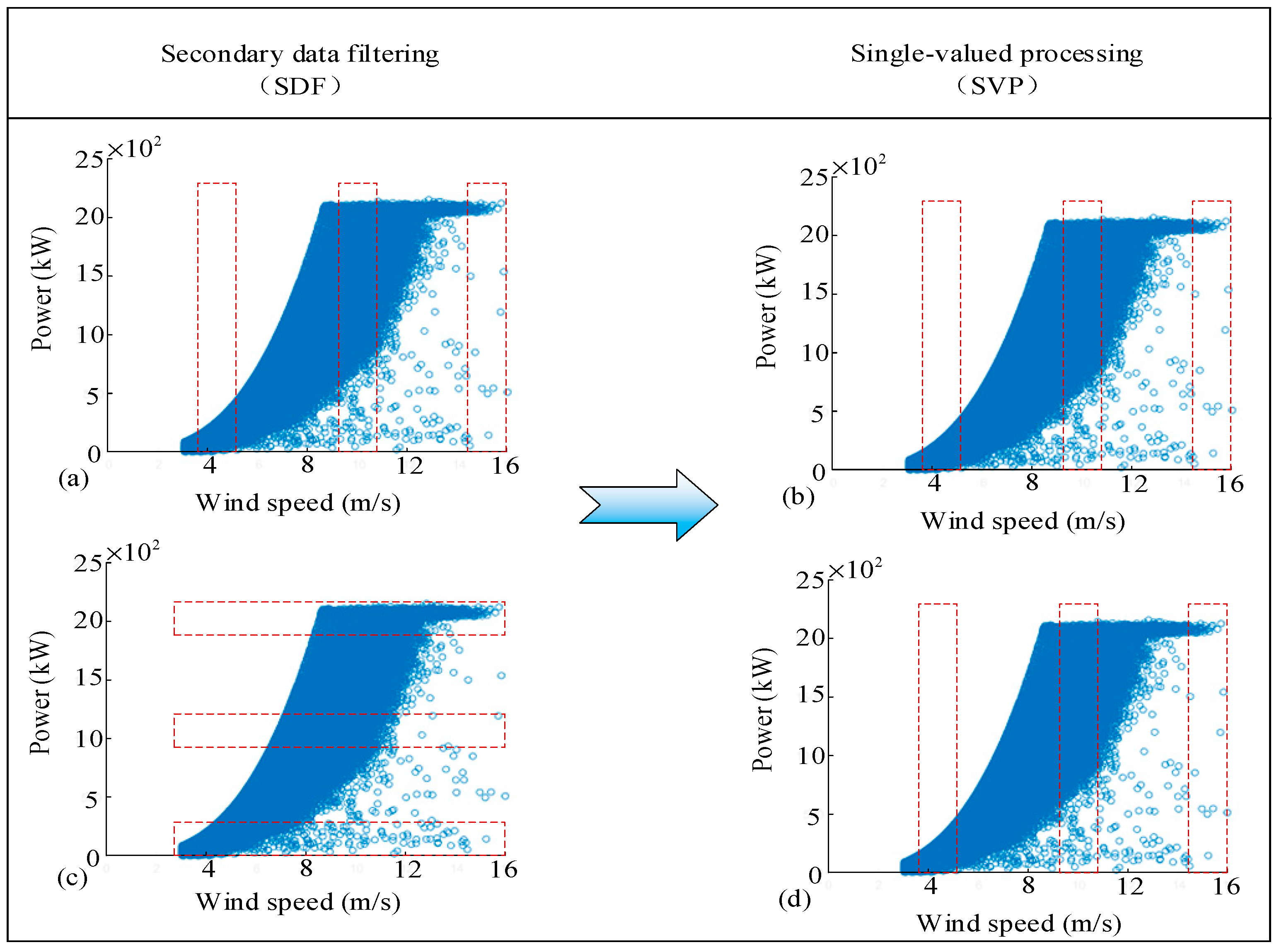
In the above data processing process, an important step is data Binning. In Stage II in Figure 6, data Binning can have different modes. For the wind speed–power curve, data Binning can be based on wind speed or power. For wind speed–rotational speed curve, data Binning can be performed based on wind speed or rotational speed. Figure 8 shows the difference between the two different Binning benchmarks, taking the wind–power curve as an example. Figure 8a shows the data Binning based on wind speed; Figure 8c shows the data Binning based on power. Different data Binning modes have an impact on the modeling of the power curve and rotational speed curve. It should be noted that in Stage III of Figure 6, only one data Binning benchmark is used, as shown in Figure 8b,d, that is, the data Binning is based on the wind speed. This is because in the process of the power curve single-valued processing, if the power benchmark is used, only one data point can be obtained above the rated wind speed, which is not applicable. The same principle is also applicable to the single-valued processing of the rotational speed curve.
As mentioned earlier, this paper constructs nine data processing methods, and the power curve and rotational speed curve obtained by different data processing methods will also be different. To better represent the effect of different methods, four indicators are proposed for comparison.
- Indicator 1 is the maximum power deviation , which means the maximum power deviation between different data processing methods corresponding to the same wind speed.
- Indicator 2 is the power fluctuation amplitude above the rated wind speed. In this region, constant power control is implemented. Theoretically, the power is a horizontal line, but the power curve processed by the actual data is fluctuating.
- Indicator 3 is the maximum rotational speed deviation , which means the maximum rotational speed deviation between different data processing methods corresponding to the same wind speed.
- Indicator 4 is the rotational speed fluctuation amplitude above the rated wind speed. In this region, constant rotational speed control is implemented. Theoretically, the rotational speed is a horizontal line, but the rotational speed curve processed by the actual data is fluctuating.
According to the definition of the maximum power deviation, its calculation expression can be written as
where, (W) and (W) represent the maximum and minimum power values obtained by different data processing methods at the same wind speed; m is the number of discrete points of the power curve within the full wind speed range, and its value is the number of wind speed data Binning.
According to the definition of the power fluctuation amplitude, its calculation expression can be written as
where, (W) is the power value using the nth data processing method when the wind speed is () (m/s); k is the number of discrete points of the power curve above the rated wind speed (constant power region); (W) is the average power obtained by the nth data processing method in the constant power area.
According to the definition of the maximum rotational speed deviation, its calculation expression can be written as
where, (rad/s) and (rad/s) represent the maximum and minimum rotational speed values obtained by different data processing methods at the same wind speed.
According to the definition of rotational speed fluctuation amplitude, its calculation expression can be written as
where, (rad/s) is the rotational speed value using the nth data processing method when the wind speed is (m/s); k is the number of discrete points of the rotational speed curve above the rated wind speed (constant power region); (rad/s) is the average rotational speed obtained by the nth data processing method in the constant power area.
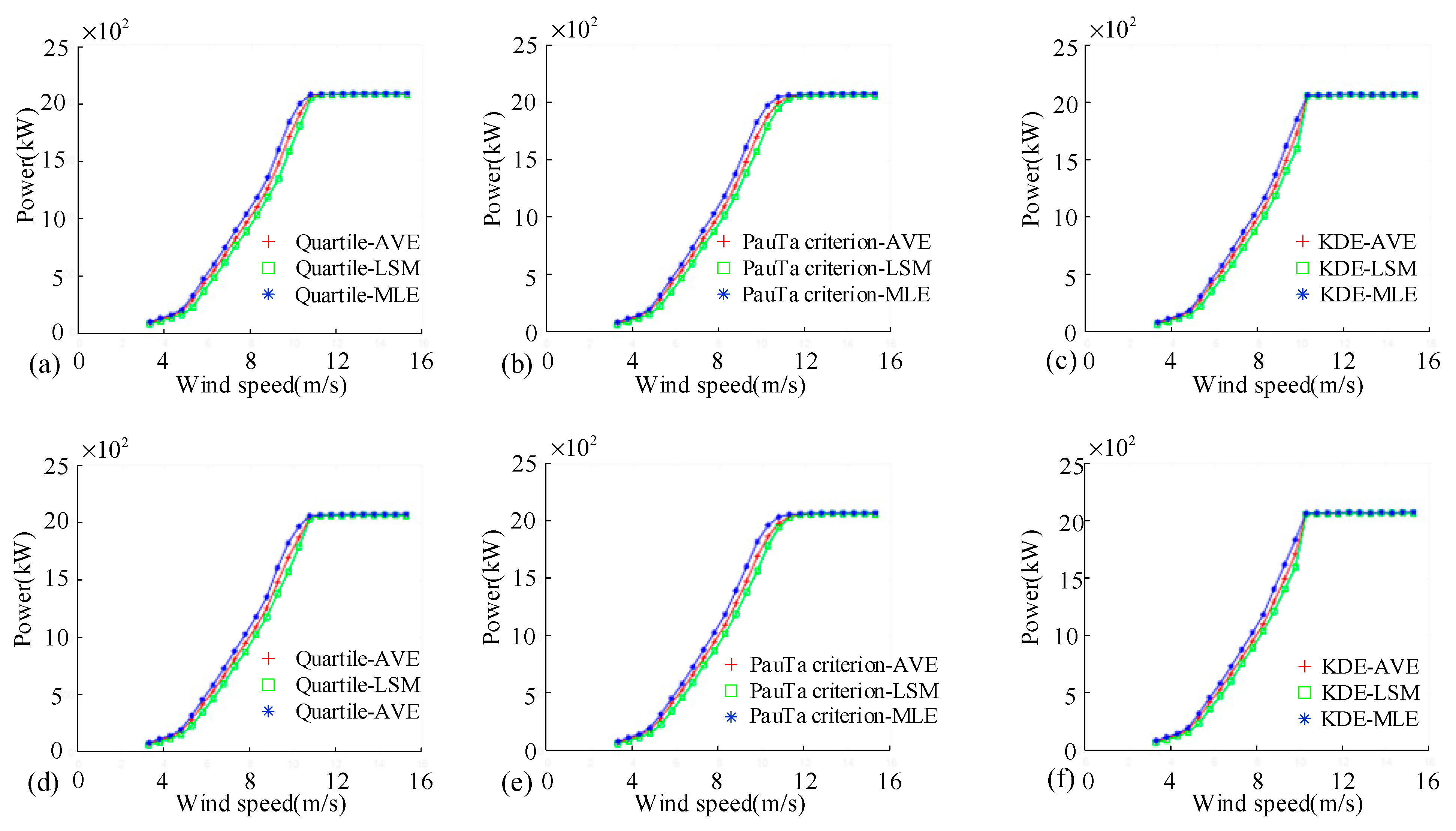
Figure 9 shows nine wind speed-power curves obtained by nine data processing methods, among which Figure 9a–c are the wind speed–power curves using wind speed data Binning, and Figure 9d–f are the wind speed–power curves using power data Binning. Table 3 shows the values of various indicators under different Binning conditions. It can be seen from the curves in Figure 9 that the rated wind speeds obtained by different data processing methods are nearly the same, and the power curves tend to be consistent overall. The maximum power deviation using the wind speed data Binning occurs when the wind speed is 11.25 m/s, between the KDE–MLE method and the Quartile–LSM method, with a maximum deviation of 236.93 kW. The maximum power deviation using power data Binning occurs when the wind speed is 10.75 m/s, also between the KDE–MLE method and Quartile–LSM method, with a maximum deviation of 120.70 kW. In general, no matter which method is used, the maximum power deviation using the power data Binning is smaller than that using the wind speed data Binning. This is because the wind speed is random, and the power has good stability. Therefore, when the power is taken as the benchmark, the interference of instantaneous wind speed can be eliminated better, and a better filtering effect can be achieved. In contrast, when the wind speed is taken as the benchmark, there will be a large deviation, which makes it not possible to obtain a better filtering effect. The maximum power fluctuation amplitude using wind speed data Binning occurs at the PauTa criterion–LSM method, with a value of 13.8%; the minimum power fluctuation amplitude occurs at the KDE–AVE method, with a value of 0.9%. The maximum power fluctuation amplitude using power data Binning also occurs at the PauTa criterion–LSM method, with a value of 17.2%; the minimum power fluctuation amplitude occurs at the KDE–MLE method, with a value of 9.3%. It shows that among the nine methods when the PauTa criterion–LSM method is used, the result of the power fluctuation amplitude is poor. In general, no matter which method is used, the power fluctuation amplitude using wind speed data Binning is better than that using power data Binning. This is because when the wind speed is above the rated wind speed, the power value is in a limited range, and it is difficult to eliminate the abnormal value of wind speed by power data Binning.
Figure 10a–c are the wind speed–rotational speed curves using the wind speed data Binning, and Figure 10d–f are the wind speed–rotational speed curves using the speed data Binning. The rotational speed curves obtained by different data processing methods tend to be consistent, and the rated speeds are nearly the same. The maximum rotational speed deviation using the wind speed data Binning occurs at the wind speed of 5.25 m/s, between the PauTa criterion–MLE method and the KDE–LSM method, and the maximum rotational speed deviation is 0.11 rad/s. The maximum rotational speed deviation using the rotational speed data Binning occurs at the wind speed of 6.25 m/s, between the KDE–MLE method and the Quartile–LSM method, and the maximum rotational speed deviation is 0.10 rad/s. The wind speed when reaching the maximum rotational speed deviation occurs at the maximum wind energy tracking stage. In general, no matter which method is used, the maximum rotational speed deviation using the power data Binning is smaller than that using the wind speed data Binning.
The maximum rotational speed fluctuation amplitude using the wind speed data Binning occurs at the KDE–MLE method, with a value of 1.5%; the minimum rotational speed fluctuation amplitude occurs at the Quartile–LSM method, with a value of 0.9%. The maximum rotational speed fluctuation amplitude using the power data Binning also occurs at the KDE–MLE method, with a value of 2.1%; the minimum rotational speed fluctuation amplitude also occurs at the Quartile–LSM method, with a value of 1.6%. No matter which method is used, the rotational speed fluctuation amplitude using the wind speed data Binning is better than that using the power data Binning.
5.2. Influence of Sliding Mode of Binning
Another critical step in the above data Binning process is the selection of sliding mode. In Stage II in Figure 6, data Binning can have different sliding modes. Discrete sliding Binning or equal-width (shoulder-to-shoulder) sliding Binning can be selected. Figure 11 shows two different sliding Binning modes. Figure 11a,b are the wind speed–power curve and the wind speed–rotational speed curve, respectively, which are processed by discrete sliding Binning. Figure 11c,d are processed by equal-width (shoulder-to-shoulder) sliding Binning.
Figure 12a–c is the wind speed–power curve obtained by selecting the discrete sliding Binning, and Figure 12d–f is the wind speed–power curve obtained by selecting the equal width (shoulder-to-shoulder) sliding Binning. Here, the Binning width of the equal width (shoulder-to-shoulder) sliding Binning is set to be 0.5 m/s. The Binning width of the discrete sliding Binning is also set to 0.5 m/s, and the sliding interval is set to 0.1 m/s. Table 4 shows the values of various indicators under different sliding Binning modes. During the discussion, the wind speed data Binning benchmark is used. From the curve in Figure 12, the rated power and rated wind speed obtained by different data processing methods are very close, and the power curve tends to be consistent. Among the three single-valued methods, the power value obtained by the LSM method is relatively small, and the power value obtained by the MLE method is relatively large. The maximum power deviation using the discrete sliding Binning occurs when the wind speed is 9.25 m/s, between the KDE–MLE method and the Quartile–LSM method, with a maximum deviation of 290.59 kW. The maximum power deviation using the equal width (shoulder-to-shoulder) sliding Binning occurs when the wind speed is 10.25 m/s, also between the KDE–MLE method and the Quartile–LSM method, with the maximum deviation of 275.90 kW. In general, no matter which method is used, the maximum power deviation using the equal width (shoulder-to-shoulder) sliding Binning is smaller than that using the discrete sliding Binning. The maximum power fluctuation amplitude using the discrete sliding Binning occurs at the PuaTa–LSM method, with a value of 1.28%; the minimum rotational speed fluctuation amplitude occurs at the Quartile–MLE method, with a value of 0.29%. The maximum power fluctuation amplitude using the equal width (shoulder-to-shoulder) sliding Binning also occurs at the PuaTa–LSM method, with a value of 1.30%; the minimum power fluctuation amplitude also occurs at the Quartile–MLE method, with a value of 0.28%. Under different sliding Binning modes, there is no obvious change in the power fluctuation amplitude obtained by the same data processing method. This is because even though the sliding mode is different, the amount of data in the Binning does not change much and has enough data. For the same filtering method, the filtering of outliers has similar effect.
Figure 13a–c is the wind speed–rotational speed curve obtained by selecting the discrete sliding Binning, and Figure 13d–f is the wind speed–rotational speed curve obtained by selecting the equal width (shoulder-to-shoulder) sliding Binning. The rotational speed curves obtained by different data processing methods tend to be consistent, and the rated speeds are nearly the same. Among the three single-valued methods, the rotational speed value obtained by the LSM method is relatively small, and the rotational speed value obtained by the MLE method is relatively large. The maximum rotational speed deviation using the discrete sliding Binning occurs when the wind speed is 5.25 m/s, between the KDE–MLE method and the Quartile–LSM method, with a maximum deviation of 0.13 rad/s. The maximum rotational speed deviation using the equal width (shoulder-to-shoulder) sliding Binning occurs when the wind speed is 5.75 m/s, also between the KDE–MLE method and the Quartile–LSM method, with the maximum deviation of 0.09 rad/s. No matter which method is used, the maximum rotational speed deviation using the equal width (shoulder-to-shoulder) sliding Binning is smaller than that using the discrete sliding Binning. The maximum rotational speed fluctuation amplitude using the discrete sliding Binning occurs at the PuaTa–LSM method, with a value of 2.84%; the minimum rotational speed fluctuation amplitude occurs at the KDE–MLE method, with a value of 2.07%. The maximum rotational speed fluctuation amplitude using the equal width (shoulder-to-shoulder) sliding Binning also occurs at the PuaTa–LSM method, with a value of 2.48%; the minimum rotational speed fluctuation amplitude occurs at the KDE–LSM method, with a value of 2.10%. This again verifies that among the nine data processing methods, the performance of the rotating speed fluctuation amplitude obtained by the PuaTa–LSM method is the worst. Among the three single-valued methods, the KDE data filtering method performs best at the constant rotational speed stage. Under different sliding Binning modes, there is no obvious change in the rotating speed fluctuation amplitude obtained by the same data processing method.
5.3. Reliability Analysis Based on ECC
As mentioned above, the rotational speed–power curve can be reconstructed from the wind-power curve and the wind–rotational speed curve. Then, the reconstructed rotational speed–power curve is compared with the rotational speed–power curve obtained from the rotational speed data and power data in the SCADA system. The calculation algorithm is described in Equation (22). The smaller the target value, the closer the reconstructed rotational speed–power curve is to the real rotational speed–power data, and the better the data pre-processing method is. This comparison is based on the energy characteristic consistency (ECC) of wind turbines described in Section 2. Here, it should be noted that the rotational speed data and power data in the SCADA system are both measured values and are relatively accurate measured values. Therefore, it can be considered that the rotational speed–power curve directly constructed from SCADA data is the actual performance curve of wind turbines.
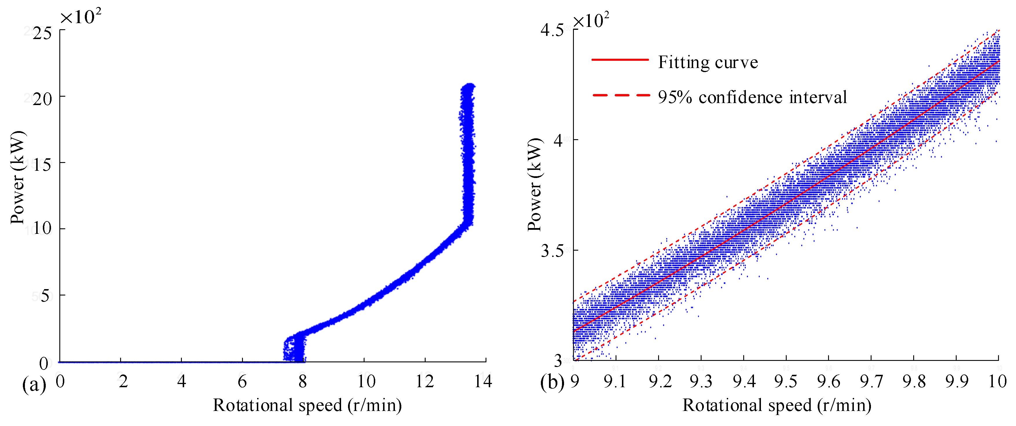
The rotational speed–power curve directly constructed from SCADA data is shown in Figure 14a. Except for a few abnormal values, most of the data are in line with the theoretical trend of the speed–power curve. Figure 14b shows the scattered data in the maximum wind energy tracking stage, and the fitting curve and confidence interval are also given in the figure. The reason for selecting the maximum wind energy tracking stage is that when wind turbines are in the startup stage and constant speed stage, the power increases (decreases) while the rotational speed remains unchanged. If these stages are included in the scope of comparison, it will cause large errors. Since the relationship between rotational speed and power is a cubic function (Equation (3)), the fitting form in the figure is a cubic polynomial. In addition, considering the existing interference data, the confidence interval is set to filter out the outliers far from the main data band, to improve the data reliability.
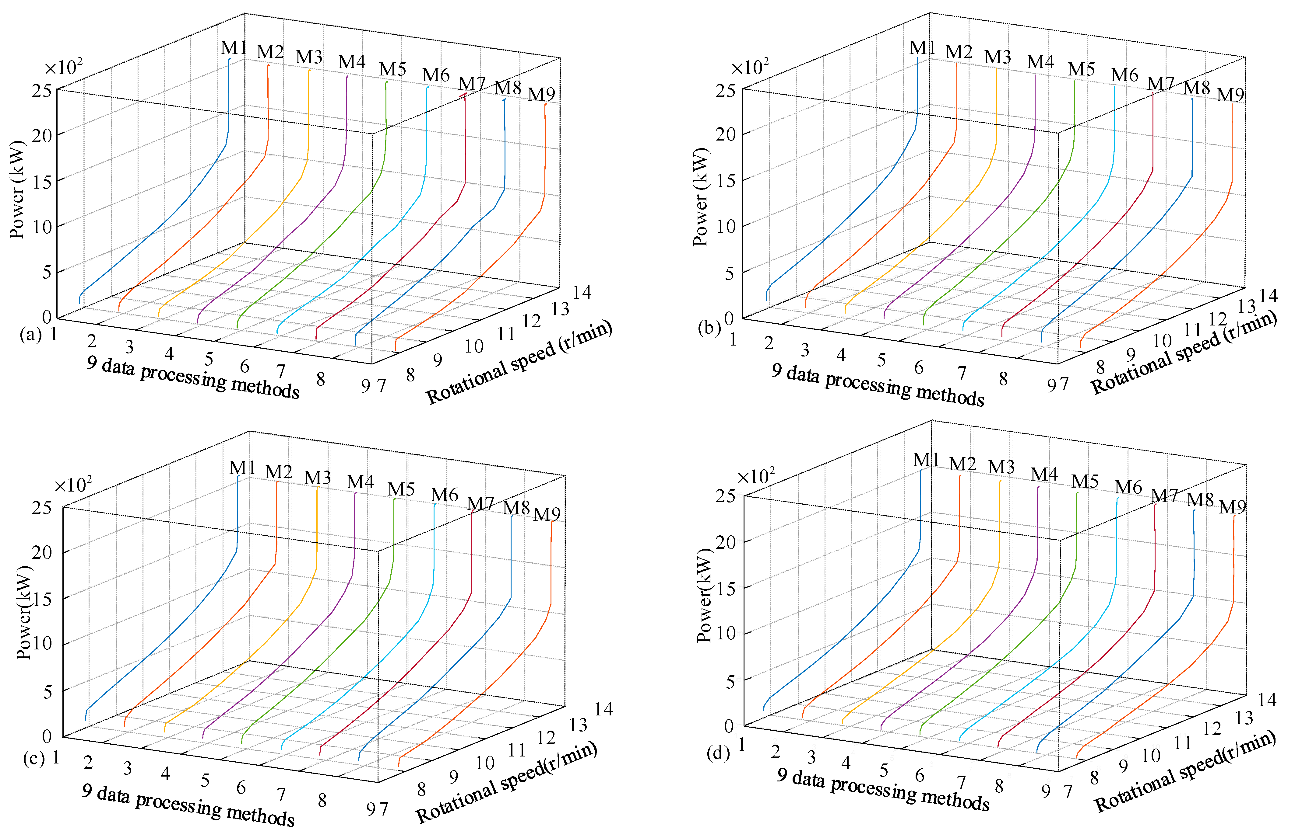
Four wind turbines are selected to verify the advantages and disadvantages of the nine data processing methods. Figure 15a shows the rotational speed–power curve of WT1, and Figure 15b–d show the rotational speed–power curve of WT2, WT3, and WT4 respectively. Table 5 shows the evaluating index s calculated from Equation (22). It can be seen from Figure 15 that the rotational speed–power curves obtained by the nine data pre-processing methods tend to be consistent, with local differences. At the same wind speed, the rotational speed and power values obtained by MLE are relatively high among the three single-valued methods. This shows that after filtering in stage II, most of the data is concentrated at the upper center level. Among the three outlier filtering methods, the power value obtained by KDE is relatively large. The rated rotational speed of WT1 is 13.42 r/min. The minimum wind speed to reach the rated rotational speed is 9.25 m/s, which occurs at three combination methods of KDE (KDE–AVE, KDE–LSM, and KDE–MLE), and the maximum wind speed is 10.25 m/s, which occurs at PuaTa–AVE. The wind speed for other methods to reach the rated rotational speed is 9.75 m/s. The rated power of WT1 is 2071.04 kW. The minimum wind speed to reach the rated power is 11.75 m/s, which occurs at three combination methods of KDE (KDE–AVE, KDE–LSM, and KDE–MLE). The maximum wind speed is 12.75 m/s, which occurs at several combination methods of PuaTa (PuaTa–AVE, PuaTa–LSM, and PuaTa–MLE). The wind speed for other methods to reach the rated power is 12.25 m/s. By analyzing the evaluating index s in Table 5, the values obtained by different data processing methods are quite different. PuaTa–LSM performed the best, with a value of 6.13 kW, while PuaTa–AVE performed the worst, with a value of 15.36 kW.
The rated rotational speed of WT2 is 13.48 r/min. The wind speed using Quartile–LSM and PuaTa–AVE to reach the rated speed is 9.75 m/s, and the wind speed for other methods is 10.25 m/s. The rated power of WT2 is 2062.72 kW. The wind speed using the three combined methods of KDE to reach the rated power is 11.75 m/s, and the wind speed for the other methods is 12.25 m/s. By analyzing the evaluating index s in Table 5, Quartile–LSM performed the best, with a value of 5.07 kW, while PuaTa–AVE performed the worst, with a value of 9.27 kW.
The rated rotational speed of WT3 is 13.50 r/min. The wind speed using three combination methods of KDE to reach the rated rotational speed is 9.25 m/s, and the wind speed for other methods is 8.75 m/s. The rated power of WT3 is 2070.83 kW. The minimum wind speed to reach the rated power is 10.25 m/s, which occurs at three combination methods of KDE. The maximum wind speed to reach the rated power is 12.25 m/s, which occurs at three combination methods of the PuaTa criterion. By analyzing the evaluating index s in Table 5, PuaTa–MLE performed the best, with a value of 8.50 kW, while PuaTa–LSM performed the worst, with a value of 12.02 kW.
The rated rotational speed of WT4 is 13.50 r/min. The wind speed using Quartile–LSM, PuaTa–AVE, and PuaTa–LSM to reach the rated rotational speed is 8.75 m/s. The wind speed for other methods is 8.25 m/s. The rated power of WT4 is 2014.55 kW. The minimum wind speed to reach the rated power is 10.75 m/s, which occurs at KDE–LSM. The maximum wind speed to reach the rated power is 12.25 m/s, which occurs at PuaTa–LSM. By analyzing the evaluating index s in Table 5, KDE–AVE performed the best, with a value of 8.88 kW, and PuaTa–LSM performed the worst, with a value of 11.08 kW.
More useful information can be found in Table 5. For example, by observing the evaluation index s of each wind turbine, the maximum value occurs in two methods, namely PauTa–AVE and PauTa–LSM. Specifically, for WT1 and WT2, the s value obtained by PauTa–AVE is the largest. For WT3 and WT4, the s value obtained by PauTa–LSM is the largest. In another scenario, the method to obtain the best evaluation index (the corresponding s value is the minimum) is also different. However, from the overall data distribution in Table 5, KDE–LSM has good performance in general. The sum of four evaluating index values obtained by KDE–LSM from four wind turbines is the smallest. By calculating the standard deviation of the evaluation indexes obtained by the same method on four wind turbines, it can be found that the performance of Quartile–MLE is the best, with a value of 1.29. The standard deviation of the evaluation indexes obtained by the KDE–LSM on four wind turbines is 1.82. An important piece of information revealed here is that no method is absolutely the best, which is related to the amount of data and observation angle.
6. Conclusions
This paper has fully explored various data pre-processing algorithms for power curve online modeling of wind turbines. The purpose is to find the most suitable algorithm. To analyze the reliability of various data processing algorithms, the novel energy characteristic consistency (ECC) is proposed for the first time. The analytical expression between the power and the wind speed measured by the nacelle anemometer is presented. This theoretically proves why the wind speed measured by the nacelle anemometer should be compensated. Moreover, the SCADA data processing is divided into three stages, namely, preliminary data filtering and compensation, secondary data filtering based on Binning, and single-valued processing based on Binnig. Different data processing algorithms are selected at different stages and finally merged into 9 data processing algorithms. Among these data processing methods, Quartile–AVE, Quartile–LSM, and Quartile–MLE have the advantage that they do not need to know the data distribution characteristics in stage II (secondary data filtering). The advantage of PauTa–AVE, PauTa–LSM, and PauTa–MLE is that if the data obey the approximate positive distribution, the outliers can be effectively eliminated at stage II. The advantage of KDE–AVE, KDE–LSM, and KDE–MLE is that when processing data in stage II, it can obtain its data distribution without prior knowledge. An evaluation method based on the energy characteristic consistency (ECC) of wind turbines is proposed which is one of the main contributions of this paper. This evaluating index quantitatively compares the reconstructed rotational speed–power curve with the actual rotational speed–power curve. The influence of sliding mode and the benchmark of Binning on data processing has been fully analyzed through four quantitative indicators. Furthermore, four wind turbines are selected to verify the advantages and disadvantages of the nine data processing methods. The results show that KDE–LSM has good performance in general. The sum of four evaluating index values obtained by KDE–LSM from four wind turbines is the smallest. The evaluating index values of the four wind turbines are 6.51 kW, 5.53 kW, 9.23 kW, and 8.96 kW, respectively, and the sum is 30.23 kW.
Author Contributions
Data processing and writing, C.Z.; paper conception, J.D.; figure design, G.L.; programming, M.L.; data processing and writing assistance, F.Z. All authors have read and agreed to the published version of the manuscript.
Funding
This work is supported by the National Natural Science Foundation of People’s Republic of China (grant number 52075164, 51975535) and the science and technology innovation Program of Hunan Province (grant number 2021RC4038).
Institutional Review Board Statement
Not applicable.
Informed Consent Statement
Not applicable.
Data Availability Statement
Not applicable.
Conflicts of Interest
The authors declare no conflict of interest.
References
- Chen, M.; Huang, W.; Ali, S. Asymmetric linkages between wind energy and ecological sustainability: Evidence from quantile estimation. Environ. Dev. 2023, 45, 100798. [Google Scholar] [CrossRef]
- Liu, F.; Wang, X.; Sun, F.; Kleidon, A. Potential impact of global stilling on wind energy production in China. Energy 2023, 263, 125727. [Google Scholar] [CrossRef]
- Dai, J.; Yang, X.; Wen, L. Development of wind power industry in China: A comprehensive assessment. Renew. Sustain. Energy Rev. 2018, 97, 156–164. [Google Scholar] [CrossRef]
- Ye, M.; Chen, H.-C.; Koop, A. Verification and validation of CFD simulations of the NTNU BT1 wind turbine. J. Wind Eng. Ind. Aerodyn. 2023, 234, 105336. [Google Scholar] [CrossRef]
- Chen, Y.; Jin, X.; Cheng, P.; Han, H.; Li, Y. Combining CFD and artificial neural network techniques to predict vortex-induced vibration mechanism for wind turbine tower hoisting. Commun. Nonlinear Sci. Numer. Simul. 2022, 114, 106688. [Google Scholar] [CrossRef]
- Ciappi, L.; Stebel, M.; Smolka, J.; Cappietti, L.; Manfrida, G. Analytical and computational fluid dynamics models of wells turbines for oscillating water column systems. J. Energy Resour. Technol. 2022, 144, 050903. [Google Scholar] [CrossRef]
- Ismail, F.B.; Al-Muhsen, N.F.O.; Hasini, H.; Kuan, E.W.S. Computational Fluid Dynamics (CFD) investigation on associated effect of classifier blades lengths and opening angles on coal classification efficiency in coal pulverizer. Case Stud. Chem. Environ. Eng. 2022, 6, 100266. [Google Scholar] [CrossRef]
- Wang, L.; Quant, R.; Kolios, A. Fluid structure interaction modelling of horizontal-axis wind turbine blades based on CFD and FEA. J. Wind Eng. Ind. Aerodyn. 2016, 158, 11–25. [Google Scholar] [CrossRef] [Green Version]
- Tang, X.; Sun, S.; Li, P.; Lu, X.; Peng, R. Aerodynamic optimization and experiment of horizontal axis wind turbine for low wind speed. Trans. Chin. Soc. Agric. Eng. 2018, 34, 218–223. [Google Scholar]
- Li, H.; Guedes Soares, C. Assessment of failure rates and reliability of floating offshore wind turbines. Reliab. Eng. Syst. Saf. 2022, 228, 108777. [Google Scholar] [CrossRef]
- Dai, J.; Li, M.; Chen, H.; He, T.; Zhang, F. Progress and challenges on blade load research of large-scale wind turbines. Renew. Energy 2022, 196, 482–496. [Google Scholar] [CrossRef]
- Satymov, R.; Bogdanov, D.; Breyer, C. Global-local analysis of cost-optimal onshore wind turbine configurations considering wind classes and hub heights. Energy 2022, 256, 124629. [Google Scholar] [CrossRef]
- Gonzalez, E.; Stephen, B.; Infield, D.; Melero, J.J. On the use of high-frequency SCADA data for improved wind turbine performance monitoring. J. Phys. Conf. Ser. 2017, 926, 012009. [Google Scholar] [CrossRef]
- Zhang, A.K.Z. Analysis of wind turbine vibrations based on SCADA data. ASME J. Sol. Energy Eng. 2017, 132, 031008. [Google Scholar]
- Dai, J.; Liu, D.; Wen, L.; Long, X. Research on power coefficient of wind turbines based on SCADA data. Renew. Energy 2016, 86, 206–215. [Google Scholar] [CrossRef]
- Chen, H.; Xie, C.; Dai, J.; Cen, E.; Li, J. SCADA Data-Based working condition classification for condition assessment of wind turbine main transmission system. Energies 2021, 14, 7043. [Google Scholar] [CrossRef]
- Zeng, H.; Dai, J.; Zuo, C.; Chen, H.; Li, M.; Zhang, F. Correlation investigation of wind turbine multiple operating parameters based on SCADA data. Energies 2022, 15, 5280. [Google Scholar] [CrossRef]
- Dao, P.B. Condition monitoring and fault diagnosis of wind turbines based on structural break detection in SCADA data. Renew. Energy 2022, 185, 641–654. [Google Scholar] [CrossRef]
- Singh, U.; Rizwan, M. SCADA system dataset exploration and machine learning based forecast for wind turbines. Results Eng. 2022, 16, 100640. [Google Scholar] [CrossRef]
- Morshedizadeh, M.; Rodgers, M.; Doucette, A.; Schlanbusch, P. A Case Study of Wind Turbine Rotor Over-Speed Fault Diagnosis Using Combination of SCADA Data, Vibration Analyses and Field Inspection. Eng. Fail. Anal. 2023, 146, 107056. [Google Scholar] [CrossRef]
- Astolfi, D.; Pandit, R.; Celesti, L.; Lombardi, A.; Terzi, L. SCADA data analysis for long-term wind turbine performance assessment: A case study. Sustain. Energy Technol. Assess. 2022, 52, 102357. [Google Scholar] [CrossRef]
- Dong, X.; Gao, D.; Li, J.; Jincao, Z.; Zheng, K. Blades icing identification model of wind turbines based on SCADA data. Renew. Energy 2020, 162, 575–586. [Google Scholar] [CrossRef]
- Dai, J.; Tan, Y.; Yang, W.; Wen, L.; Shen, X. Investigation of wind resource characteristics in mountain wind farm using multiple-unit SCADA data in Chenzhou: A case study. Energy Convers. Manag. 2017, 148, 378–393. [Google Scholar] [CrossRef] [Green Version]
- Yao, Q.; Zhu, H.; Xiang, L.; Su, H.; Hu, A. A novel composed method of cleaning anomy data for improving state prediction of wind turbine. Renew. Energy 2023, 204, 131–140. [Google Scholar] [CrossRef]
- Yang, W.; Court, R.; Jiang, J. Wind turbine condition monitoring by the approach of SCADA data analysis. Renew. Energy 2013, 53, 365–376. [Google Scholar] [CrossRef]
- Marti-Puig, P.; Blanco-M, A.; Cárdenas, J.J.; Cusidó, J.; Solé-Casals, J. Effects of the pre-processing algorithms in fault diagnosis of wind turbines. Environ. Model. Softw. 2018, 110, 119–128. [Google Scholar] [CrossRef]
- Long, H.; Xu, S.; Gu, W. An abnormal wind turbine data cleaning algorithm based on color space conversion and image feature detection. Appl. Energy 2022, 311, 118594. [Google Scholar] [CrossRef]
- Wang, Y.; Wang, J.; Li, Z.; Yang, H.; Li, H. Design of a combined system based on two-stage data preprocessing and multi-objective optimization for wind speed prediction. Energy 2021, 231, 121125. [Google Scholar] [CrossRef]
- Morrison, R.; Liu, X.; Lin, Z. Anomaly detection in wind turbine SCADA data for power curve cleaning. Renew. Energy 2022, 184, 473–486. [Google Scholar] [CrossRef]
- Zheng, L.; Hu, W.; Min, Y. Raw wind data preprocessing: A data-mining approach. IEEE Trans. Sustain. Energy 2014, 6, 11–19. [Google Scholar] [CrossRef]
- Dai, J.; Cao, J.; Zhang, F.; Liu, D.; Shen, X. Data pre-processing method and its evaluation strategy of SCADA data from wind farm. Acta Energ. Sol. Sin. 2017, 38, 2597–2604. [Google Scholar]
- Zhao, Y.; Ye, L.; Wang, W.; Sun, H.; Ju, Y.; Tang, Y. Data-Driven Correction Approach to Refine Power Curve of Wind Farm Under Wind Curtailment. IEEE Trans. Sustain. Energy 2018, 9, 95–105. [Google Scholar] [CrossRef]
- Ouyang, T.; Kusiak, A.; He, Y. Modeling wind-turbine power curve: A data partitioning and mining approach. Renew. Energy 2017, 102, 1–8. [Google Scholar] [CrossRef]
- Guan, J.; Lin, J.; Guan, J.; Mokaramian, E. A novel probabilistic short-term wind energy forecasting model based on an improved kernel density estimation. Int. J. Hydrogen Energy 2020, 45, 23791–23808. [Google Scholar] [CrossRef]
Figure 1.
Wind turbines and performance curves.

Figure 2.
ECC of wind turbines.

Figure 3.
Power curves based on different wind speeds.

Figure 4.
Mapping relationship between wind speed and power.

Figure 5.
Preliminary data filtering principle. (a) Quartile method; (b) PauTa criterion; (c) KDE method.
Figure 5.
Preliminary data filtering principle. (a) Quartile method; (b) PauTa criterion; (c) KDE method.

Figure 6.
Synthesis of data processing methods.

Figure 7.
Data pre-processing methods and process.

Figure 8.
Different Binning benchmarks. (a) using binning to process wind speed in SDF; (b) using binning to process wind speed in SVP; (c) using binning to process power in SDF; (d) using binning to process wind speed in SVP.
Figure 8.
Different Binning benchmarks. (a) using binning to process wind speed in SDF; (b) using binning to process wind speed in SVP; (c) using binning to process power in SDF; (d) using binning to process wind speed in SVP.

Figure 9.
Influence of Binning benchmark on wind-power curve. (a) wind-power curves obtained by binning wind speed data using three Quartile-based methods; (b) wind-power curves obtained by binning wind speed data using three PauTa-based methods; (c) wind-power curves obtained by binning wind speed data using three KDE-based methods. (d) wind-power curves obtained by binning power data using three Quartile-based methods. (e) wind-power curves obtained by binning power data using three PauTa-based methods. (f) wind-power curves obtained by binning power data using three KDE-based methods.

Figure 10.
Influence of Binning benchmark on wind–rotational speed curve. (a) wind speed and rotational speed curves obtained by binning wind speed data using three Quartile-based methods; (b) wind speed and rotational speed curves obtained by binning wind speed data using three PauTa-based methods; (c) wind speed and rotational speed curves obtained by binning wind speed data using three KDE-based methods. (d) wind speed and rotational speed curves obtained by binning power data using three Quartile-based methods. (e) wind speed and rotational speed curves obtained by binning power data using three PauTa-based methods. (f) wind speed and rotational speed curves obtained by binning power data using three KDE-based methods.

Figure 11.
Different sliding Binning modes. (a) wind-power scatted relationship obtained by DSB mode; (b) wind-power scatted relationship obtained by SSB mode; (c) wind speed and rotational speed scatted relationship obtained by DSB mode; (d) wind speed and rotational speed scatted relationship obtained by SSB mode.

Figure 12.
Influence of sliding Binning mode on wind–power curve. (a) wind–power curves obtained by selecting DSB mode using three Quartile-based methods; (b) wind–power curves obtained by selecting DSB mode using three PauTa-based methods; (c) wind–power curves obtained by selecting DSB mode using three KDE-based methods; (d) wind–power curves obtained by selecting SSB mode using three Quartile-based methods; (e) wind–power curves obtained by selecting SSB mode using three PauTa-based methods; (f) wind–power curves obtained by selecting SSB mode using three KDE-based methods.

Figure 13.
Influence of sliding Binning mode on wind–rotational speed curve. (a) wind speed and rotational speed curves obtained by selecting DSB mode using three Quartile-based methods; (b) wind speed and rotational speed curves obtained by selecting DSB mode using three PauTa-based methods; (c) wind speed and rotational speed curves obtained by selecting DSB mode using three KDE-based methods; (d) wind speed and rotational speed curves obtained by selecting SSB mode using three Quartile-based methods; (e) wind speed and rotational speed curves obtained by selecting SSB mode using three PauTa-based methods; (f) wind speed and rotational speed curves obtained by selecting SSB mode using three KDE-based methods.

Figure 14.
Rotational speed–power curve directly constructed from SCADA data. (a) rotational speed–power curve in full range; (b) rotational speed–power curve in the maximum wind energy tracking stage.
Figure 14.
Rotational speed–power curve directly constructed from SCADA data. (a) rotational speed–power curve in full range; (b) rotational speed–power curve in the maximum wind energy tracking stage.

Figure 15.
Rotational speed-power curve of four wind turbines. (a) rotational speed–power curve of WT1; (b) rotational speed–power curve of WT2; (c) rotational speed–power curve of WT3; (d) rotational speed–power curve of WT4.
Figure 15.
Rotational speed-power curve of four wind turbines. (a) rotational speed–power curve of WT1; (b) rotational speed–power curve of WT2; (c) rotational speed–power curve of WT3; (d) rotational speed–power curve of WT4.


Table 1.
Data pre-processing methods.
| Preliminary Data Filtering and Compensation | Secondary Data Filtering Based on Binning | Single-Valued Processing Based on Binnig | |||
|---|---|---|---|---|---|
| Preliminary data filtering | Quartile method | Average method (AVE) | |||
| PauTa criterion | Least square method (LSM) | ||||
| Wind data compensation | KDE method | Maximum likelihood estimation (MLE) | |||
Table 2.
Data pre-processing methods.
| Scatter Plot Based on Raw Data | Preliminary Data Filtering and Compensation | Secondary Data Filtering Based on Binning Partition |
|---|---|---|
 |  |  |
 |  |  |
Table 3.
Indicators of two kinds of data Binning benchmarks.
| (kW) | (%) | (%) | (rad/s) | (%) | (%) | |
|---|---|---|---|---|---|---|
| Wind speed data Binning | 236.93 | 13.8 | 0.9 | 0.11 | 1.5 | 0.9 |
| Power speed data Binning | 120.70 | 17.2 | 9.3 | 0.10 | 2.1 | 1.6 |
Table 4.
Indicators of two kinds of sliding Binning modes.
| (kW) | (%) | (%) | (rad/s) | (%) | (%) | |
|---|---|---|---|---|---|---|
| DSB | 290.59 | 1.30 | 0.28 | 0.13 | 2.84 | 2.07 |
| SSB | 275.90 | 1.28 | 0.29 | 0.09 | 2.48 | 2.10 |
Table 5.
Evaluating index s based on ECC (kW).
| Quartile-AVE | Quartile-LSM | Quartile-MLE | PauTa-AVE | PauTa-LSM | PauTa-MLE | KDE-AVE | KDE-LSM | KDE-MLE | |
|---|---|---|---|---|---|---|---|---|---|
| WT1 | 7.44 | 10.37 | 10.35 | 15.36 | 6.13 | 10.18 | 7.47 | 6.51 | 7.81 |
| WT2 | 5.38 | 5.07 | 7.33 | 9.27 | 5.21 | 7.18 | 5.76 | 5.53 | 6.49 |
| WT3 | 11.13 | 9.42 | 9.15 | 9.47 | 12.02 | 8.5 | 10.45 | 9.23 | 9.76 |
| WT4 | 9.65 | 8.91 | 9.65 | 11.05 | 11.08 | 11.07 | 8.88 | 8.96 | 9.98 |
Disclaimer/Publisher’s Note: The statements, opinions and data contained in all publications are solely those of the individual author(s) and contributor(s) and not of MDPI and/or the editor(s). MDPI and/or the editor(s) disclaim responsibility for any injury to people or property resulting from any ideas, methods, instructions or products referred to in the content. |
© 2023 by the authors. Licensee MDPI, Basel, Switzerland. This article is an open access article distributed under the terms and conditions of the Creative Commons Attribution (CC BY) license (https://creativecommons.org/licenses/by/4.0/).
Share and Cite
MDPI and ACS Style
Zuo, C.; Dai, J.; Li, G.; Li, M.; Zhang, F. Investigation of Data Pre-Processing Algorithms for Power Curve Modeling of Wind Turbines Based on ECC. Energies 2023, 16, 2679. https://0-doi-org.brum.beds.ac.uk/10.3390/en16062679
AMA Style
Zuo C, Dai J, Li G, Li M, Zhang F. Investigation of Data Pre-Processing Algorithms for Power Curve Modeling of Wind Turbines Based on ECC. Energies. 2023; 16(6):2679. https://0-doi-org.brum.beds.ac.uk/10.3390/en16062679
Chicago/Turabian StyleZuo, Chengming, Juchuan Dai, Guo Li, Mimi Li, and Fan Zhang. 2023. "Investigation of Data Pre-Processing Algorithms for Power Curve Modeling of Wind Turbines Based on ECC" Energies 16, no. 6: 2679. https://0-doi-org.brum.beds.ac.uk/10.3390/en16062679
Note that from the first issue of 2016, this journal uses article numbers instead of page numbers. See further details here.