
Fast Well Control Optimization with Two-Stage Proxy Modeling

Department of Geoscience and Petroleum, Norwegian University of Science and Technology, 7031 Trondheim, Norway
*
Author to whom correspondence should be addressed.
Energies 2023, 16(7), 3269; https://0-doi-org.brum.beds.ac.uk/10.3390/en16073269
Submission received: 23 February 2023
/
Revised: 29 March 2023
/
Accepted: 3 April 2023
/
Published: 6 April 2023
(This article belongs to the Special Issue Artificial Intelligence/Machine Learning Applications in the Oil and Gas Industry)
Abstract
:Waterflooding is one of the methods used for increased hydrocarbon production. Waterflooding optimization can be computationally prohibitive if the reservoir model or the optimization problem is complex. Hence, proxy modeling can yield a faster solution than numerical reservoir simulation. This fast solution provides insights to better formulate field development plans. Due to technological advancements, machine learning increasingly contributes to the designing and building of proxy models. Thus, in this work, we have proposed the application of the two-stage proxy modeling, namely global and local components, to generate useful insights. We have established global proxy models and coupled them with optimization algorithms to produce a new database. In this paper, the machine learning technique used is a multilayer perceptron. The optimization algorithms comprise the Genetic Algorithm and the Particle Swarm Optimization. We then implemented the newly generated database to build local proxy models to yield solutions that are close to the “ground truth”. The results obtained demonstrate that conducting global and local proxy modeling can produce results with acceptable accuracy. For the optimized rate profiles, the R2 metric overall exceeds 0.96. The range of Absolute Percentage Error of the local proxy models generally reduces to 0–3% as compared to the global proxy models which has a 0–5% error range. We achieved a reduction in computational time by six times as compared with optimization by only using a numerical reservoir simulator.
1. Introduction
Numerical reservoir simulation (NRS) is one of the most essential aspects of reservoir engineering. NRS is highly relied upon for the modeling of fluid flow in porous media. This implies that a reservoir is better when sufficient data are acquired to develop a reservoir model through NRS. Using NRS, fluids can be more efficiently extracted from the underground to meet the global energy demand. However, NRS suffers from computational issues, despite today’s advanced computing power. This limitation is still not entirely addressed, especially when many details are included in building the NRS model. Concerning this, numerous measures are proposed, including proxy modeling.
Proxy modeling pertains to the modeling of a substitute for a base paradigm, namely NRS. Such an approach can provide a fast solution when the decision-making is urgent. There are different examples of proxy modeling available for employment. In this case, the machine learning (ML) technique is one of them. In general, ML can be perceived as a computer algorithm that is built to deduce a pattern or relationship between the input variables and the output provided [1]. Some prevalent examples of ML include artificial neural networks, support vector machines, and gradient boosting machines. These methods have been demonstrated to be successful in establishing proxy models. Regarding this, some literature presented the use of an ensemble of neuro-fuzzy networks as ML-based proxy models in several aspects of reservoir engineering, including carbon, capture, and storage [2] and shale analytics [3].
Apart from these, a variant of the gradient boosting machine, e.g., extreme gradient boosting machine (XGBoost), was implemented for fast analysis of well placements in a heterogeneous reservoir [4]. The articles [5,6] also discussed the use of some more advanced ML methods in simulating the behavior of reservoirs and production trends, which is an important criterion to be manifested by a proxy model. The potential implementation of ML methods in proxy modeling was also further highlighted in the domain of secondary recovery. Waterflooding is one of the most prevalent secondary recovery techniques. Aside from its economical employment [7], it has been well-received in the oil and gas industry due to its ability to maintain the reservoir pressure, prevent subsidence, and simultaneously increase the oil recovery from oil fields. Regarding the technicality of waterflooding, “voidage replacement” has been a common parameter to guide water injection, where the total volume of production is equal to the total volume of injection. The challenge of using a voidage replacement ratio (ratio of the injected to the produced fluid volumes) with a fixed injector location is the allocation of the water injection for each well.
Changing the injection operations can optimize the waterflooding performance. These operations include the well control adjustment in which the net present value (NPV) is set to be the objective function. Conventionally, NRS is used to obtain the result for each water injection scenario. For a full-field scenario, using NRS will be time-consuming to maximize the objective function, especially if the geology of the reservoir is sophisticated or the dimension of optimization variables is high. Therefore, ML-based proxy models are suggested to mitigate the computational challenges. Several previous works [8,9] have established a methodology in this context. Nonetheless, the efficiency of the methodology in resolving the optimization problem with higher dimensionality still requires improvement. One of the potential solutions lies in the establishment of two different classes of proxy models, namely global and local proxy models, as discussed in [10,11]. Fundamentally, local proxy models aim at refining the quality of proxy models in which solutions closer to the “true” optimal can be determined.
Furthermore, to conduct a successful waterflooding optimization, an optimization algorithm is another essential tool. There are two main types of algorithms, e.g., gradient-based and gradient-free. In recent studies of optimization algorithms, gradient-free algorithms have gained increasing attention due to their ability to converge to the global optimal [12]. The nature-inspired algorithm is the epitome of gradient-free algorithms. Its successful integration with the ML-based proxy models has been displayed in several pieces of literature in reservoir and production engineering [13,14,15]. In this study, two optimization algorithms are used: the Genetic Algorithm (GA) and the Particle Swarm Optimization (PSO). These algorithms are only applied to determine the optimal sets of well control under waterflooding. These algorithms also illustrated good potential to be used as training algorithms in data-driven modeling [16,17].
In this paper, we aim to illustrate how ML and nature-inspired algorithms can be coupled with the two-stage proxy modeling to optimize waterflooding. A benchmark model (UNISIM-I-D) was used to demonstrate that global and local proxy modeling could be used to replicate the behavior of a real reservoir. The UNISIM-I-D model was created based on Namorado Field, located in Campos Basin in Brazil. The proxy models are developed using the multi-layer perceptron (MLP). These proxy models were initiated to replicate the NRS and coupled with the above-mentioned algorithms for well control optimization. The proxy models were built using selected geological properties, time, and output from the NRS. Using the Latin Hypercube Sampling (LHS) method, which was proposed by McKay et al. [18], multiple injection scenarios were created and divided into the training set and the blind validation set. NRS was performed on the injection scenarios to obtain the simulation results. After a successful training and the validation test of the proxy models, the simulation results could be generated without using NRS. Using the results from the global proxy model, the local proxy model was trained based on the retrieved samples of optimization results. With this method, the optimization result was obtained by using the local proxy model without the requirement to run the repetitive process of optimization. Using the global and local proxy models, the optimized water injection control for the UNISIM-I-D model was determined with higher computational efficiency.
Following this introduction, Section 2 of this paper discusses the details of the UNISIM-I-D model. Section 3 and Section 4 respectively explain the algorithms and the ML method applied. Thereafter, Section 5 expounds the integration of the concepts presented to scaffold the establishment of the methodology presented. Section 6 comprises a discussion on the results obtained from this work. The concluding remarks can be found in Section 7.
2. Reservoir Description
The UNISIM-I-D model was created on the Namorado Field, located in the Campos Basin in Brazil with known properties [19]. With the benchmark model, it is possible to ensure the applicability of developed reservoir management methodologies to real reservoirs. In this study, we used the upscaled model to decrease the computational effort for multiple scenarios. The grid cell resolution of the upscaled model is 100 × 100 × 8 m, discretized into a corner point grid 81 × 58 × 20 cells, with a total of 36,739 active total cells.
2.1. Static Properties Description
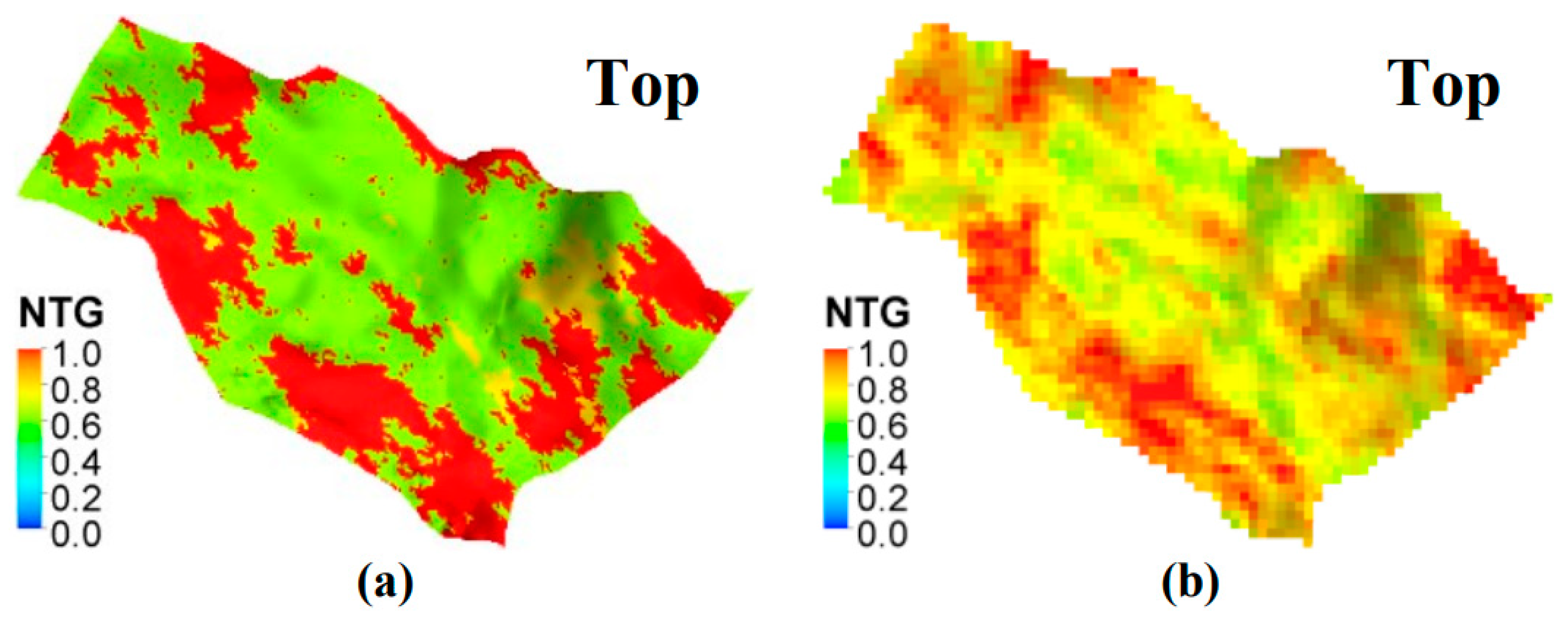
The UNISIM-I-D model facies distribution is reflected based on the net-to-gross distribution. The original fine model has the following rules to set the net-to-gross (NTG) based on the facies shown in Table 1. The facies modeling is defined using the Sequential Indicator Simulation with a vertical trend [20].
Class 0 is defined as reservoir facies with good properties whereas classes 1 and 2 are the medium reservoir properties. Class 3 is defined as non-reservoir. The reservoir active grid is upscaled and results in a continuous distribution of the NTG (Figure 1).
Figure 1 shows that after upscaling, the NTG became continuous due to the nature of the arithmetic volume-weighted method. The method is used to maintain the hydrocarbon volume constant during flow simulation.
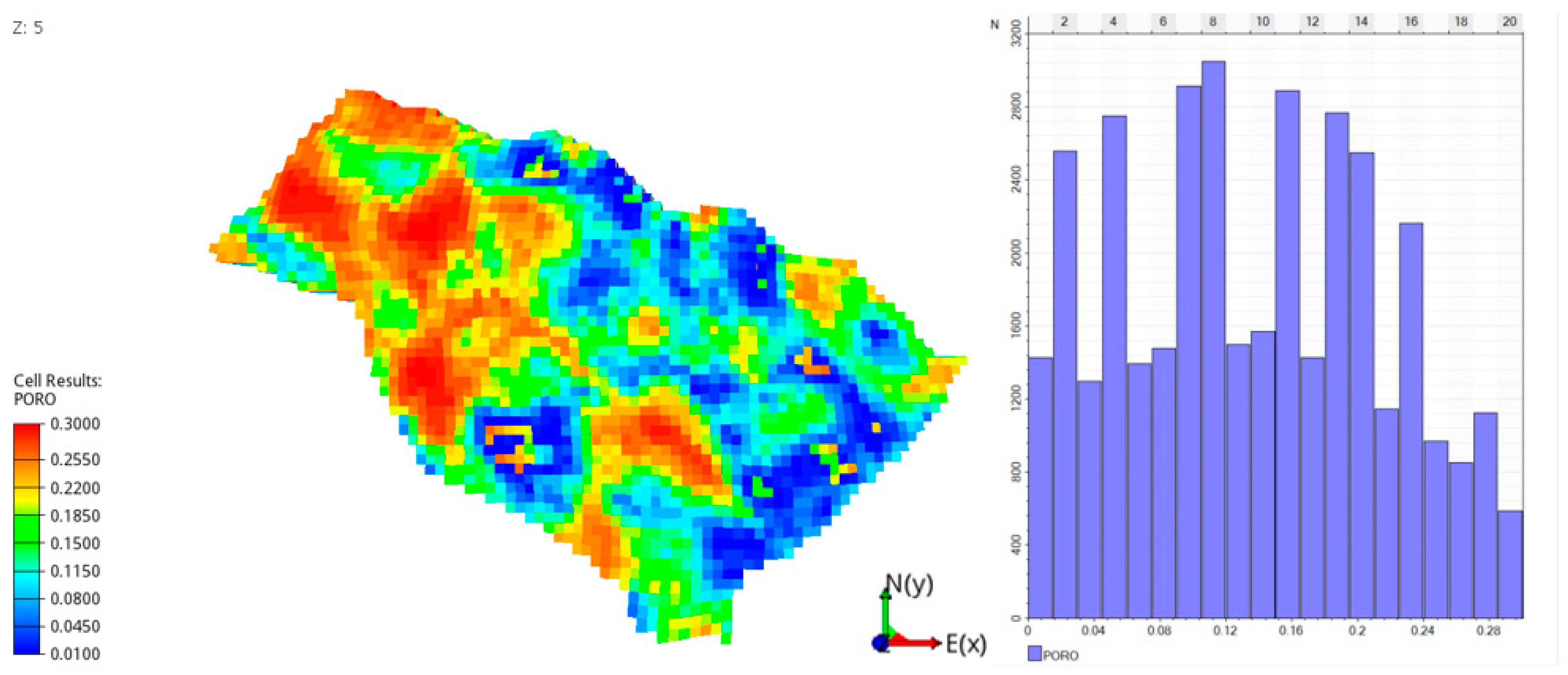
The effective porosity model is derived from the density log and shaliness of the properties. After the effective porosity is modeled from log data, it is distributed to the whole model using the Sequential Gaussian Simulation (SGS) [21]. After the porosity is modeled on the fine grid, it is upscaled using the same method as NTG upscaling. The results of upscaled porosity are shown in Figure 2.
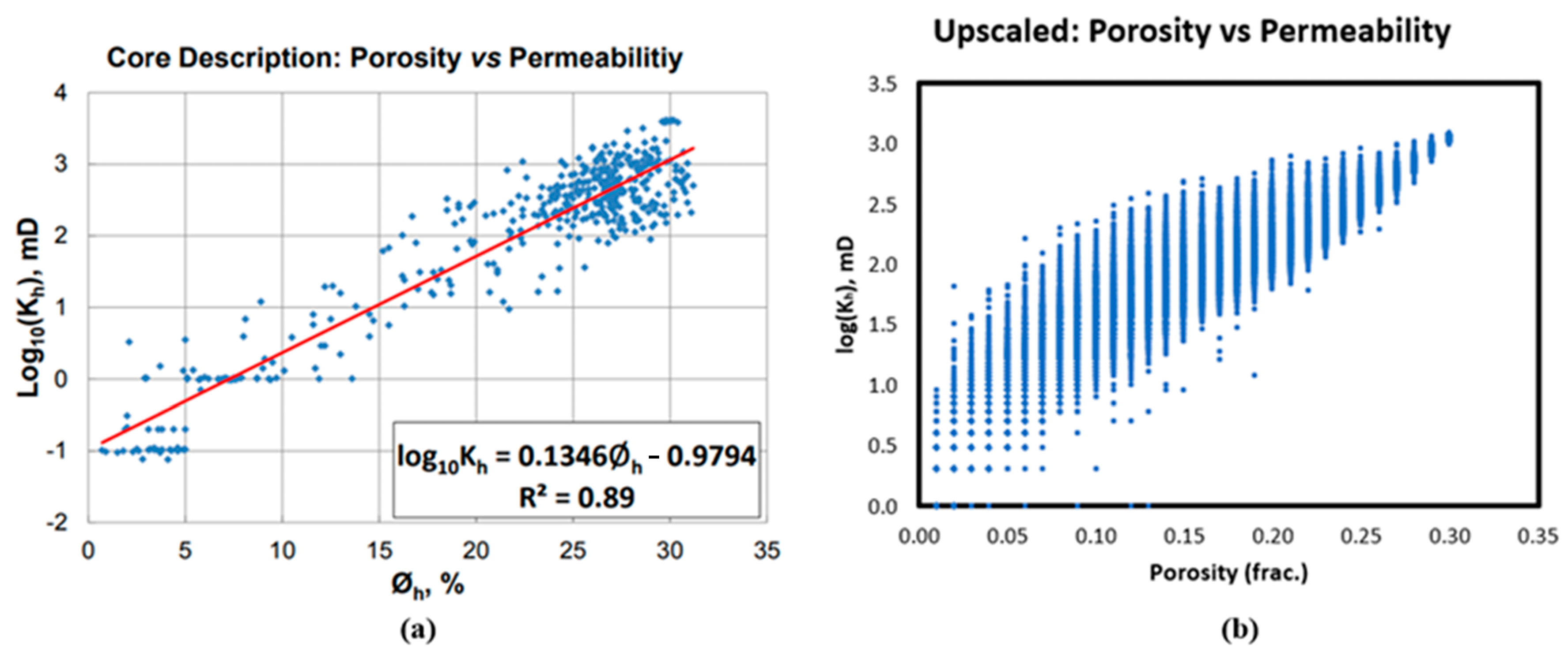
The permeability model was initially derived from the core analysis data, and a relationship between porosity and permeability was established (Figure 3). This horizontal permeability is distributed to the model using the correlation, while the vertical permeability is defined by using a multiplier (which ranges from 0 to 1.5) times the horizontal permeability. The permeability was upscaled by using the flow-based upscaling technique, FLOWSIM [22]. The results of the porosity and the horizontal permeability relationship of the upscaled case is depicted in Figure 3b.
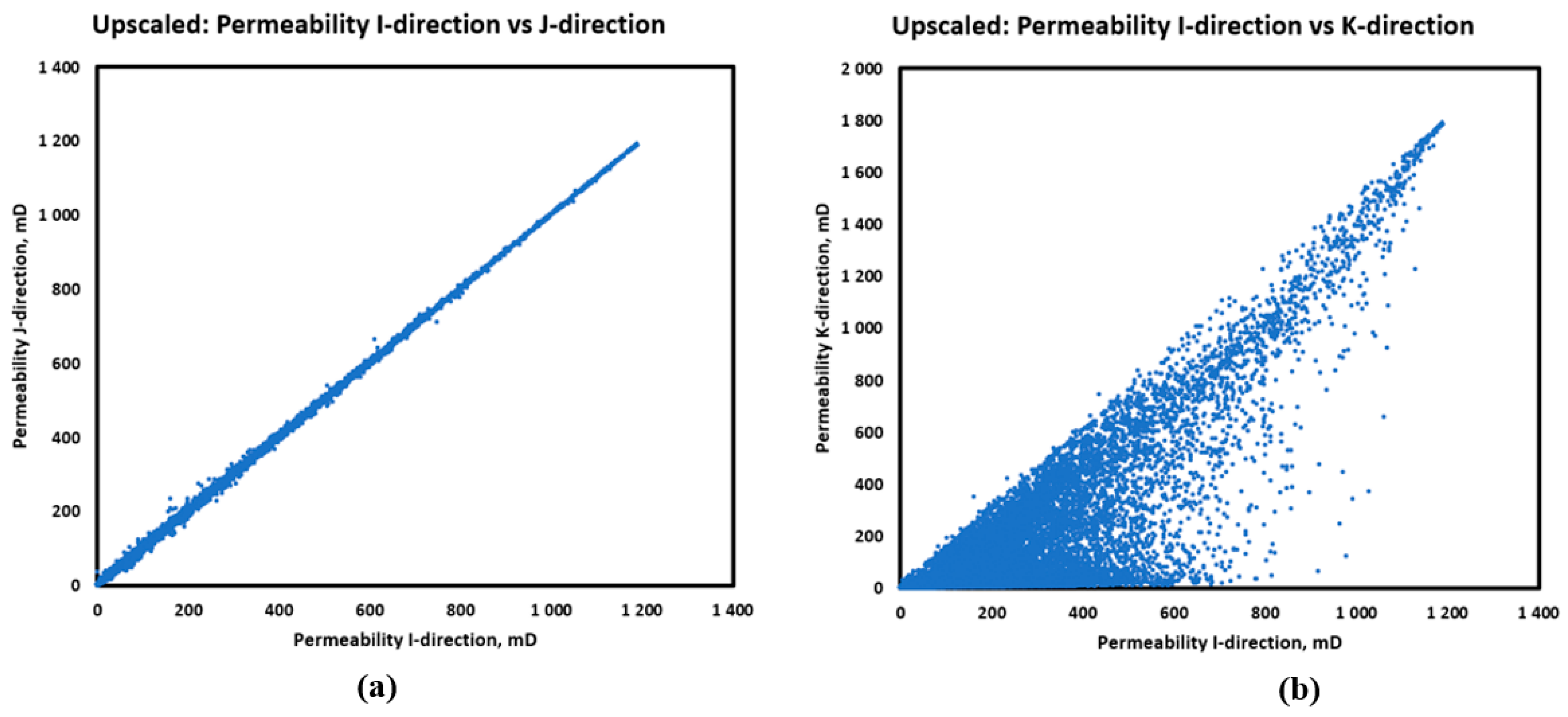
Due to the upscaling method, the horizontal permeability has slightly different values in I and J directions. Meanwhile, the relationship between the vertical and the horizontal permeability is scattered due to the different grid resolution in vertical direction. Figure 4 shows the relationship between the horizontal and the vertical permeabilities.
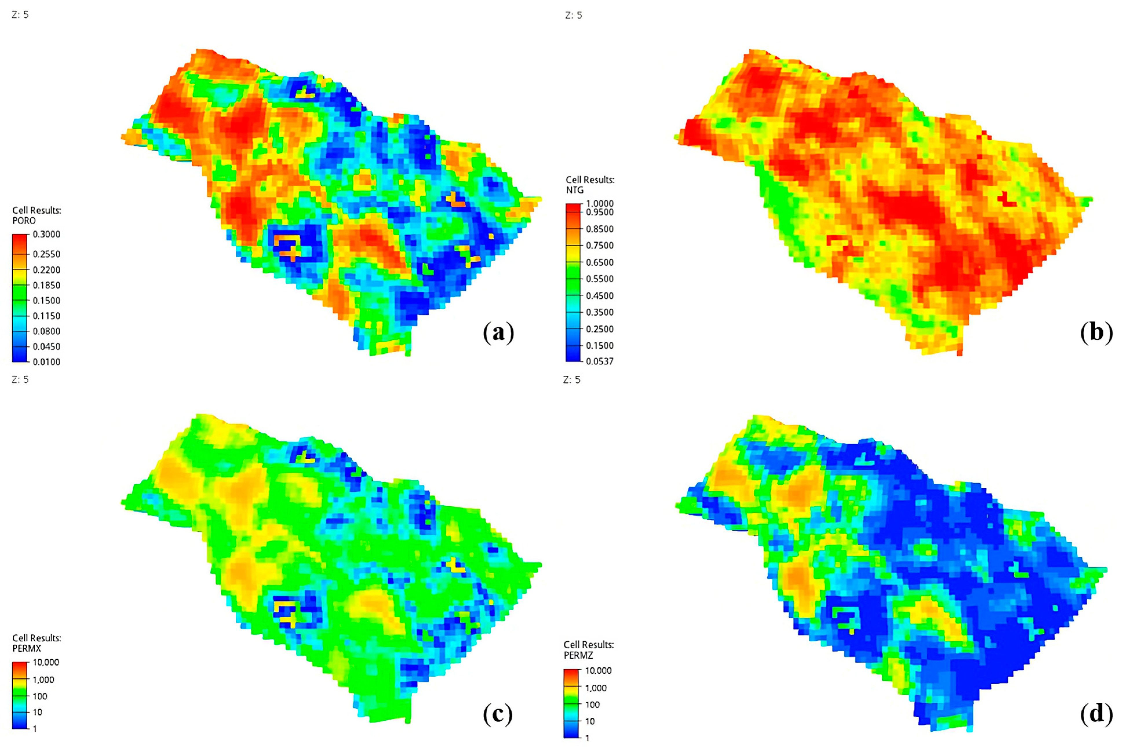
The final static properties used in this study are shown in Figure 5.
2.2. Dynamic Properties Description
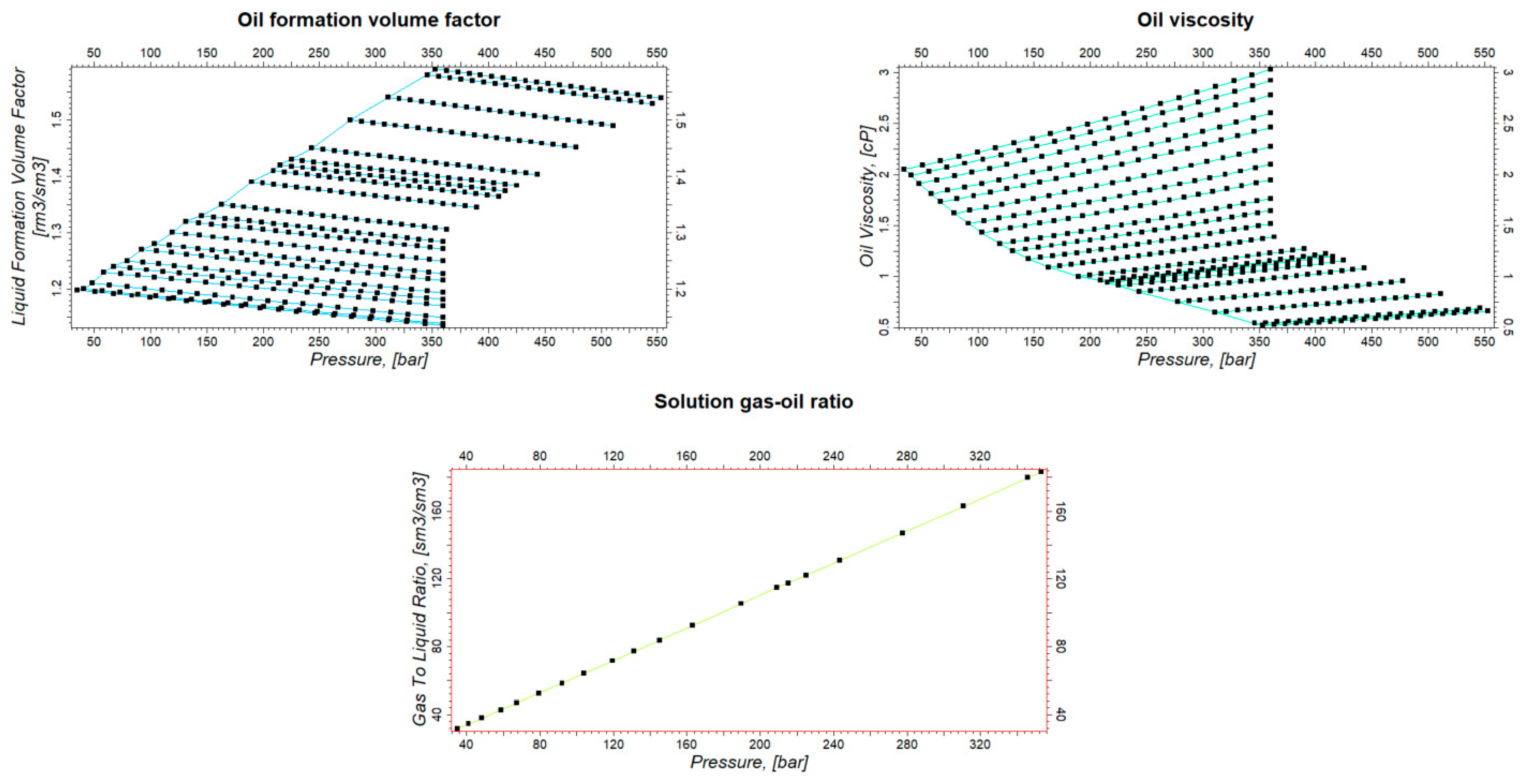
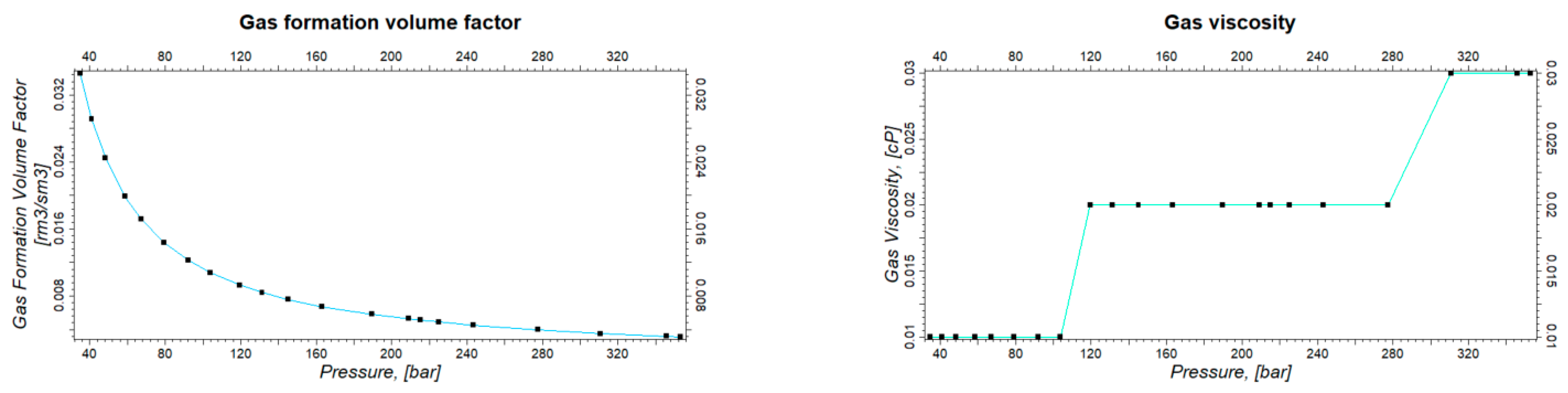
In this section, the fluid properties and fluid-rock interaction properties used in the simulation are defined. The fluid model used in the simulation is the Black Oil model with the initialization of the oil phase, the dissolved gas and the water phase. Figure 6 shows the oil properties and Figure 7 demonstrates the gas properties used in the model.
The water properties are defined in Table 2.
2.3. Initialization
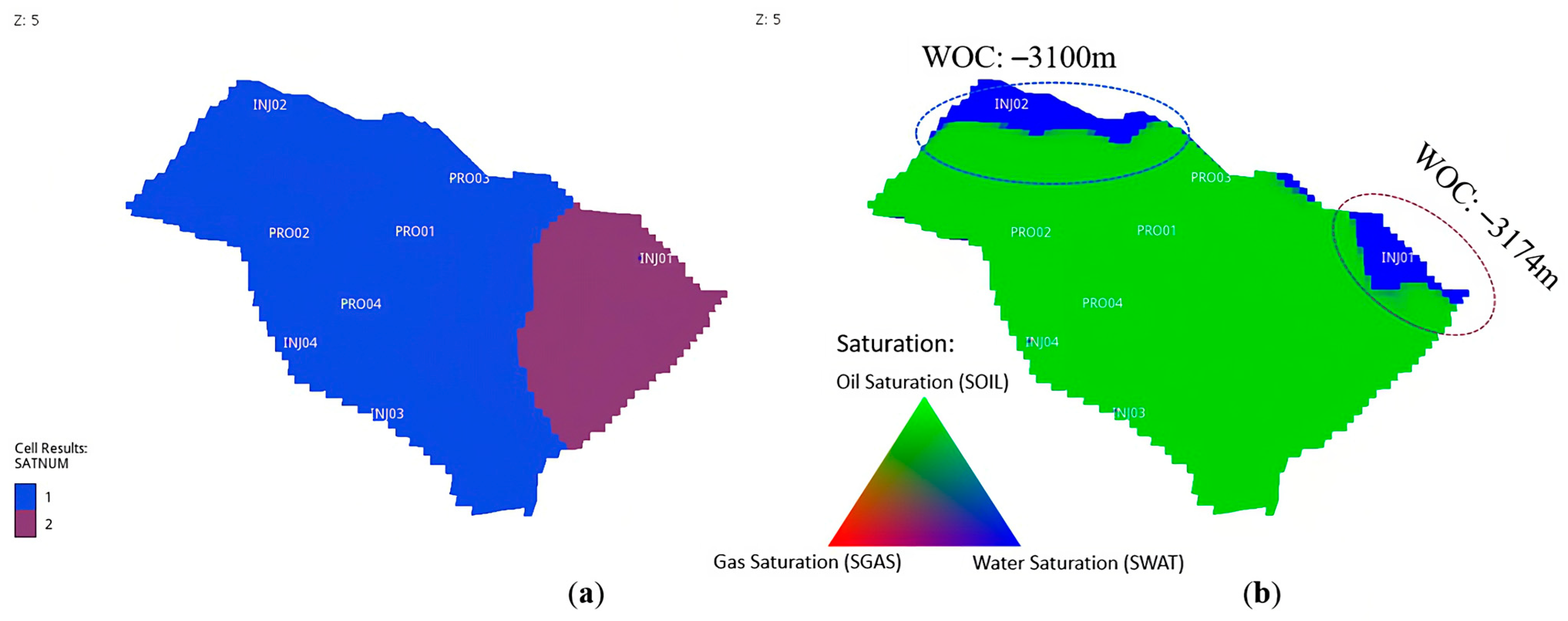
The initialization of the model is conducted by defining two regions with different water-oil contacts. The region boundary is defined by the normal fault shown in Figure 10a. The horst (blue area) has a higher water-oil contact at the depth −3100 m than the graben (magenta are) with water-oil contact at the depth −3174 m, as shown in Figure 10. The initial pressure is defined based on the reference point at depth of 3000 m where the pressure is 320.68 bara. Figure 10b shows the distribution of the initial fluid saturation with the different water-oil contacts for both regions.
3. Algorithms
Regarding the selection of mathematical algorithms, nature-inspired algorithms, specifically the Genetic Algorithm (GA) and the Particle Swarm Optimization (PSO), were preferred due to their structural simplicity and successful implementation in several articles [8,9,14]. These algorithms are derivative-free, implying that computation or approximation of gradient is unnecessary. They also present a good capability of eluding premature convergence. This is because they accomplish a good balance between exploration and exploitation in optimization. Exploration aims at diversifying the solution over the search space. Exploitation targets to leverage the search for solution over the local region (a more refined search space).
GA, proposed by Holland [26], is one of the population-based metaheuristic algorithms. Its formulation relies heavily upon the Darwinism Theory of Evolution. GA, in general, implements different types of genetic operators when it comes to the exploration and exploitation of the solution (search) space. Fundamentally, an individual solution is encoded as a string, that is known as a chromosome. Therefore, an initial population of chromosomes will be generated as potential solutions. The quality of each chromosome is evaluated by employing an objective function (also known as fitness). These chromosomes will undergo the genetic operators, for instance, selection, crossover, elitism, and mutation over several iterations. During the selection process, several chromosomes are chosen as parents to yield new offspring. Then, elitism ensures the survival of the best chromosome (highest fitness) which can be inherited in the next generation. Crossover involves the exchange of certain parts (also termed “genes”) of chromosomes to produce new ones. Mutation modifies certain genes of chromosomes to elude convergence to the local optima [27]. Mathematically, the chromosome population will be subject to these genetic operators for some iterations until the stopping criterion is met. The final chromosome with the highest fitness is treated as the final solution.
PSO is another example of the population-based algorithms that was implemented in this work. PSO was formulated by Kennedy and Eberhart [28], according to the simulation of a moving stock of birds or a school of fish. In this aspect, an individual solution is perceived as the particle, in which the initial population of particles (a swarm of particles) is randomly generated as potential solutions. The quality of each particle is assessed using an objective function. As PSO commences, the position and velocity of each particle are randomly initialized. Throughout the iterations, a particle recognizes the previous optimal value of the objective function. The respective position vector is the local best position (pbest). The global best position (gbest) is the best position of particles achieved hitherto in the swarm. At every iteration, the motion of particles is dictated by three parameters, namely cognitive factors, social factors, and inertia weight. Generally, the cognitive factor enables the attraction of particles towards the pbest. The social factor aids in attraction towards the gbest. Inertia weight could be initialized to improve convergence. The pbest and gbest are determined iteratively to update the velocity at the current step. As the velocity at the next iteration is evaluated, the update on the position of a particle at the next iteration is performed. Over some iterations, each particle updates its position via the minimization of the objective function until the stopping criterion is reached.
4. Machine Learning
Machine learning (ML) is defined as a computer algorithm that can derive inferences in the pattern of data provided. There are numerous examples of ML techniques, including support vector machines, random forests, and artificial neural networks (ANN). ANN is one of the most popular methods of ML that has been applied extensively. Its mechanism primarily resembles the neural system in human brains. Mathematically, it comprises different fundamental components, including layers, activation functions, and nodes. The layers are input, hidden, and output. Each layer consists of several nodes that are represented by weights and biases. Starting from the input layer, weights and biases are consecutively interconnected layer to layer. Thereafter, the respective product will be fed into a preselected activation function to yield a new value that will propagate to the next layer. This process of propagation continues until it reaches the output layer. For the relevant details, refer to the literature [29]. Application of ANN generally gravitates to the development of data-driven models which are used for prediction and/or optimization. There are also different variants of ANN, such as multilayer perceptron (MLP), recurrent neural network (RNN), and convolutional neural network (CNN). In this work, only MLP is considered due to its successful use in resolving engineering problems.
5. Proxy Modeling and Optimization Problem
To establish proxy models, we need to be cognizant of the functions of the proxy models before proceeding into the development phase. In our study, we formulate a waterflooding optimization problem, in which the pertinent objective function is set to be the net present value (NPV). This NPV function is mathematically expressed in Equation (1). The control vector is represented by u and the field rates are indicated by Q, in which the subscripts refer to the types of fluids. P refers to the price or cost of fluid produced/injected. ntotal is the total number of timesteps whereas ti refers to the cumulative time until timestep i. refers to the timestep difference between the time i and the previous timestep. Such an optimization problem resonates with some of our previous works [8,9]. However, one of the distinctive differences pertains to the number of optimization variables (decision variables) included. In the case of this optimization, NPV is maximized every 365 days by optimally adjusting each injection rate (within the range of 0 Sm3/day and 2500 Sm3/day) and bottomhole pressure (BHP) of each producer (within 175 bar and 200 bar). The total production period lasts for 9125 days.
Since the UNISIM-I-D reservoir model comprises four injectors and four producers, this results in 200 variables (8 variables/timestep × 25 timesteps) to be optimized to achieve a higher NPV. Based on the NPV function, we assume that the produced gas will be sold. Regarding the economic parameters, the oil price is 503.2 USD/m3, the cost of handling produced water and injecting water are 62.9 USD/m3 and 50.32 USD/m3, respectively, and the gas price is 0.265 USD/m3. The interest rate is 0.10 per year. From the NPV function, we need to develop models that can predict the values of the Field Oil Production Rate (FOPR), Field Water Production Rate (FWPR), Field Water Injection Rate (FWIR), and Field Gas Production Rate (FGPR) at each timestep. Keeping in mind our investigation and previous studies [8,17,30], we decided to build three different proxy models, which can forecast Field Liquid Production Rate (FLPR), Field Water Cut (FWCT), and FWIR. FLPR and FWIR are in the units of Sm3/day whereas FWCT is expressed in a fraction. These proxy models provide the necessary values to compute the NPV. It is essential to know that FGPR (Sm3/day) can be obtained by multiplying FOPR by the constant gas-oil-ratio Rs, which is 113.45 Sm3/Sm3.
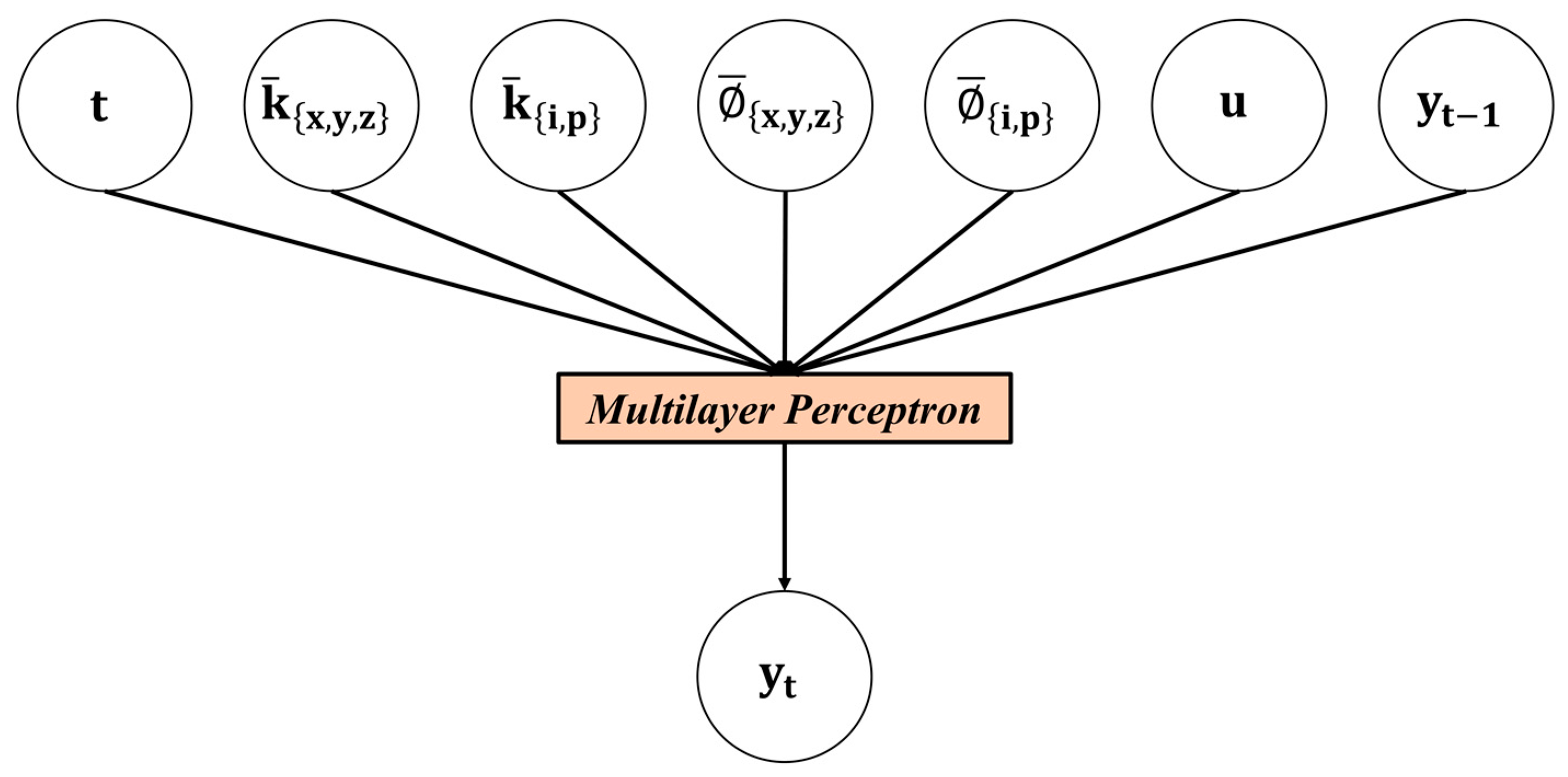
Proxy modeling can be perceived as establishing a relationship between the input and the output variables. Our previous studies and some literature suggest that integrating static and dynamic properties can increase the reliability of the proxy models. Therefore, we have formulated the mathematical function of the proxy models, as shown in Figure 11. In Figure 11, represents the arithmetic mean of grid block permeability for each layer in x-, y-, and z-directions. refers to the arithmetic mean of grid block porosity for every layer. and respectively correspond to the arithmetic mean of permeability and porosity of the perforated grid blocks for each injector and producer. Parameters u and respectively refer to control variables and cumulative time (days) until the current timestep. and correspond to output at previous and current timestep. As discussed, there are 20 layers and 8 wells in the UNISIM-I-D model, and this yields 112 static inputs. Considering the dynamic inputs, such as the number of days, 8 control variables, and output at the previous timestep, there are 122 input variables.
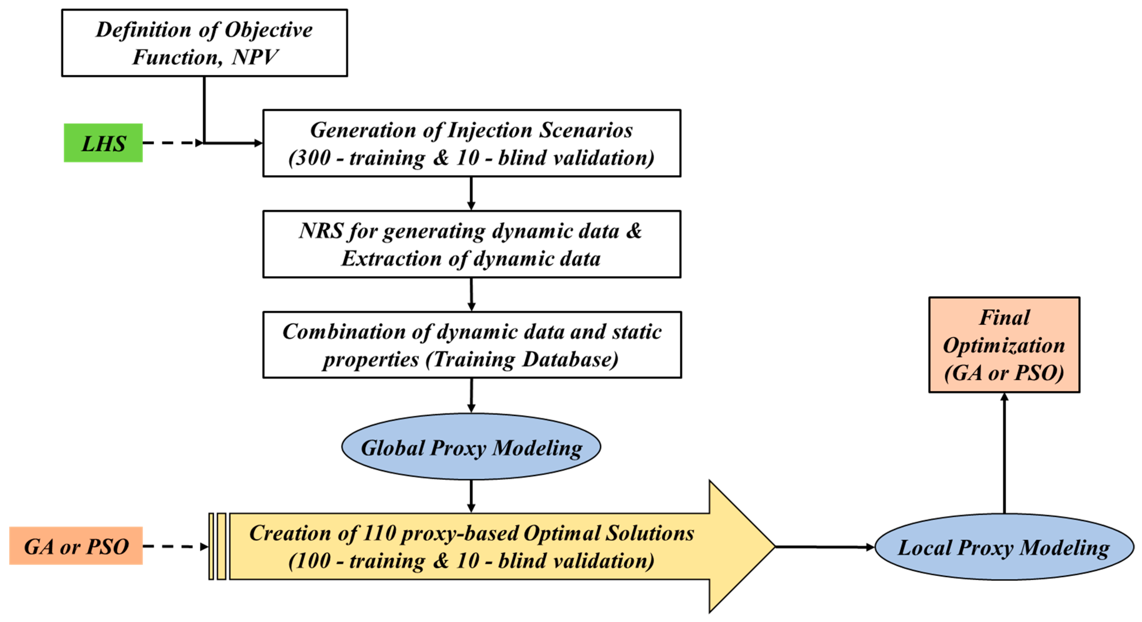
Understanding the objective of the optimization problem and the formulation of proxy models provides a clear direction to proceed into the workflow, as shown in Figure 12. This workflow involves the design of two types of proxy models which we correspondingly term as the Global Proxy Models and the Local Proxy Models. As displayed in the workflow, Latin Hypercube Sampling (LHS) is initiated to create 310 control scenarios. These 300 scenarios are fed into NRS to generate a training database for Global Proxy Modeling. The other 10 scenarios are applied to create the database for blind validation. The maximum NPV resulting from these scenarios is 5456.70 million USD. Before proceeding to the training process, the database is normalized to be between 0 and 1 based on the maximum and minimum data, as discussed in [9]. After developing the global proxy models, they are coupled with GA or PSO to generate the database for local proxy modeling. The topologies of global and local proxy models are decided via a trial-and-error approach, which is portrayed in Table 5. The terms “Local Proxy-GA” and “Local Proxy-PSO” in the table imply that the local proxy models are built from the database generated using the global proxy models coupled with GA and PSO for optimization, respectively. In Table 5, the number of hidden nodes applies to each hidden layer. Moreover, the activation function in the output layer for each proxy model is linear. The training uses the algorithm Adam, also known as Adaptive Moment Estimation [31], iterations of 2000, a learning rate of 0.001, and a tolerance of 10−6. The early stopping feature is activated. The validation fraction is set to 1/9. The remaining parameters are the default values, as suggested in Scikit-Learn [32].
The inertia weight is 0.80 whereas the cognitive and social learning factors are both parameterized as 1.05. r1 and r2 are sampled from a uniform distribution between 0 and 1. For the GA, the crossover probability is 0.8, the mutation probability is 0.8, the elite ratio is 1/30, the parents’ portion is 0.6, and the type of crossover is two-point. The abovementioned parameters for both GA and PSO were initialized via a trial-and-error approach. For both algorithms, the number of optimization iteration is 200 and the population size is 30.
As the training and blind validation results of global proxy models illustrate good results, these models are coupled with metaheuristic algorithms to conduct the waterflooding optimization. The optimization is run 110 times (indicating 110 optimal scenarios in which 100 scenarios are for training and the other 10 are for blind validation) and the resulting optimal solutions (control variables) are sent back to the simulator to create a training database for local proxy modeling. For this, the calculated NPV is ensured to exceed the abovementioned maximum NPV. When the local proxy models illustrate good results of training and blind validation, these models are implemented for the final optimization. The final optimization is performed 200 times for further analysis. The relevant findings are summarized and discussed in the following section.
6. Results and Discussion
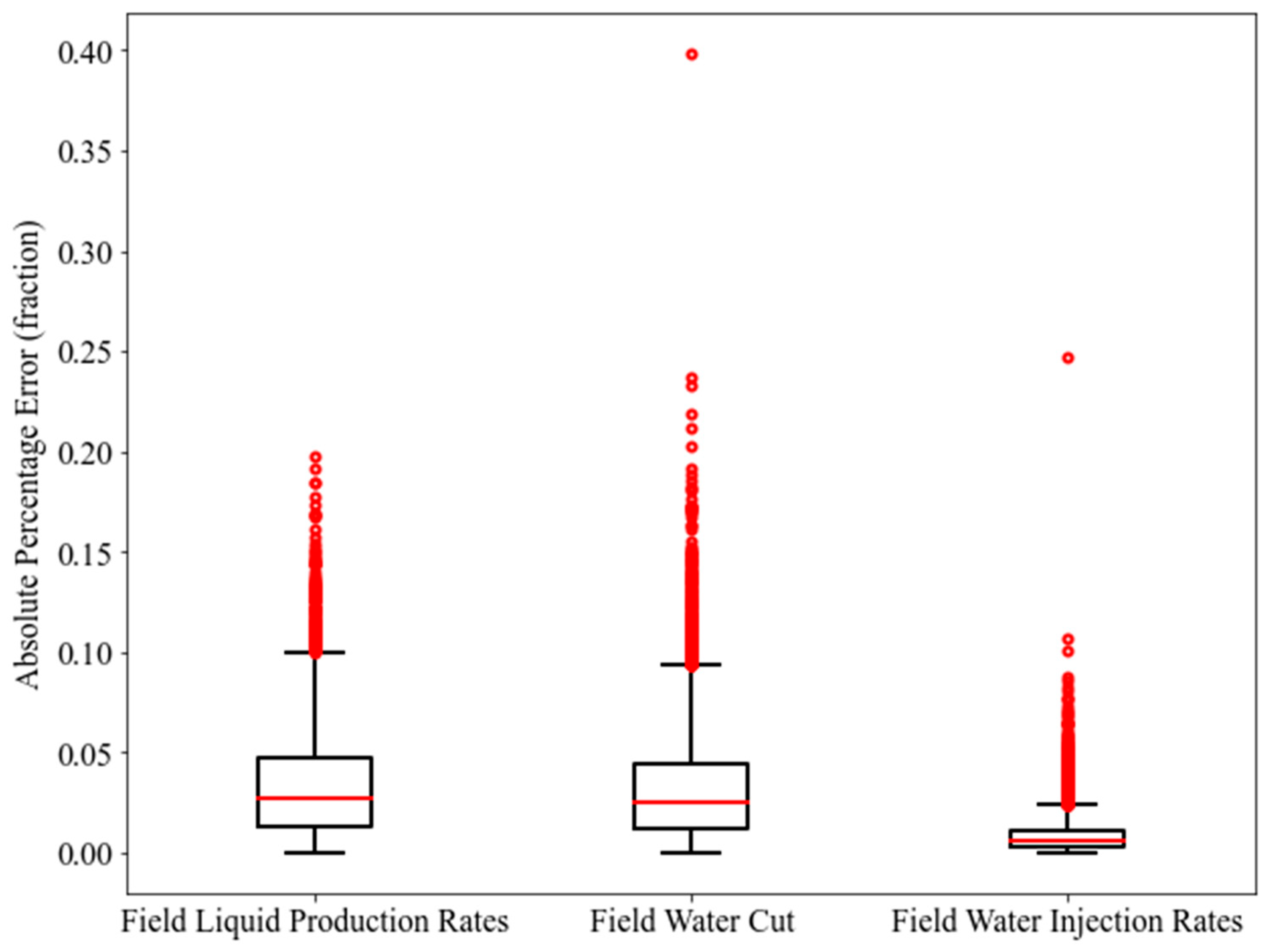
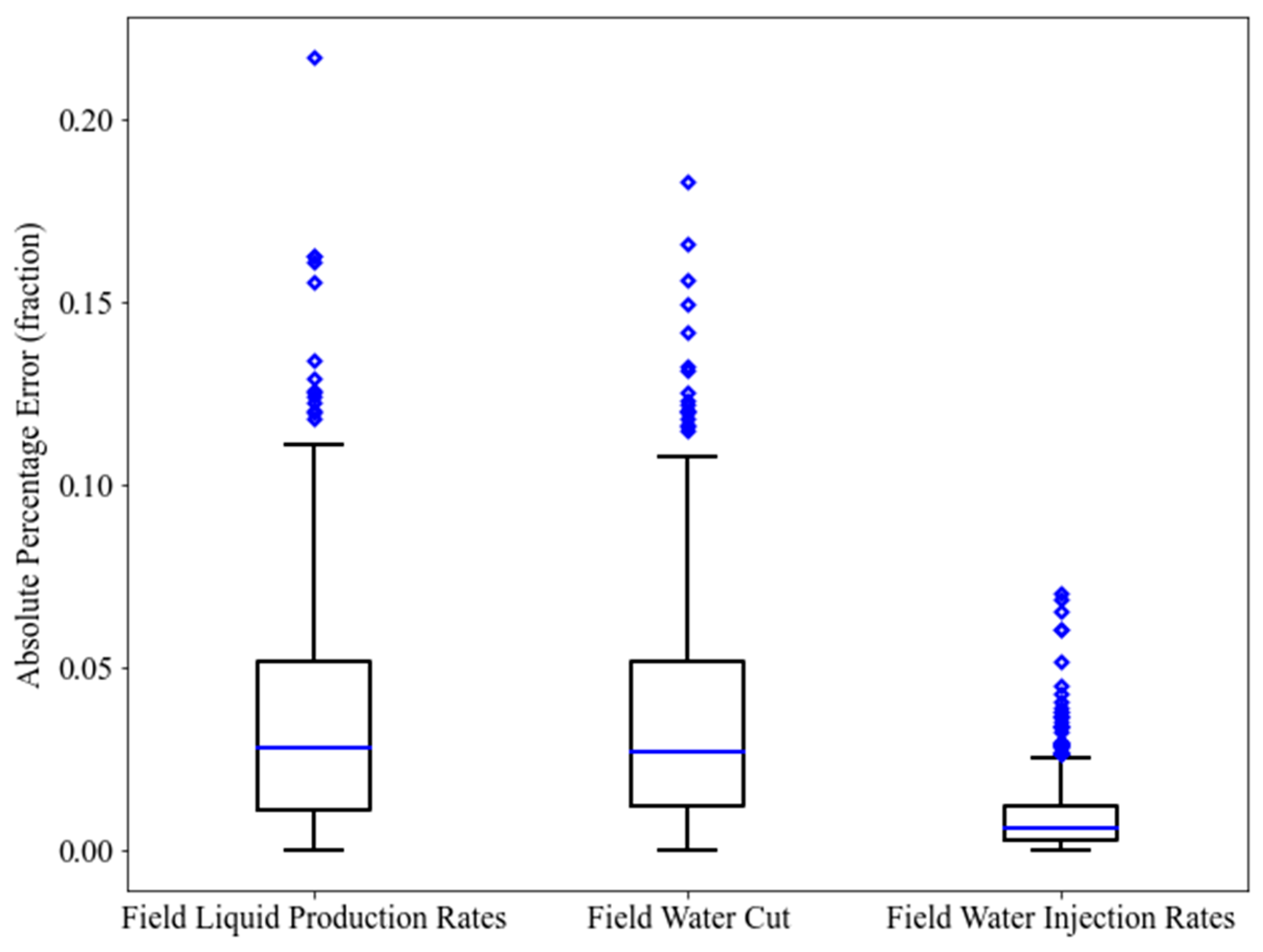
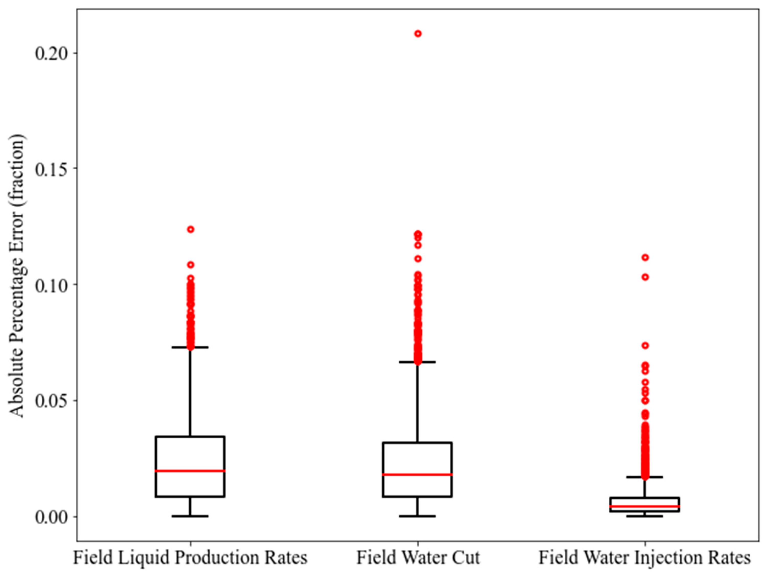
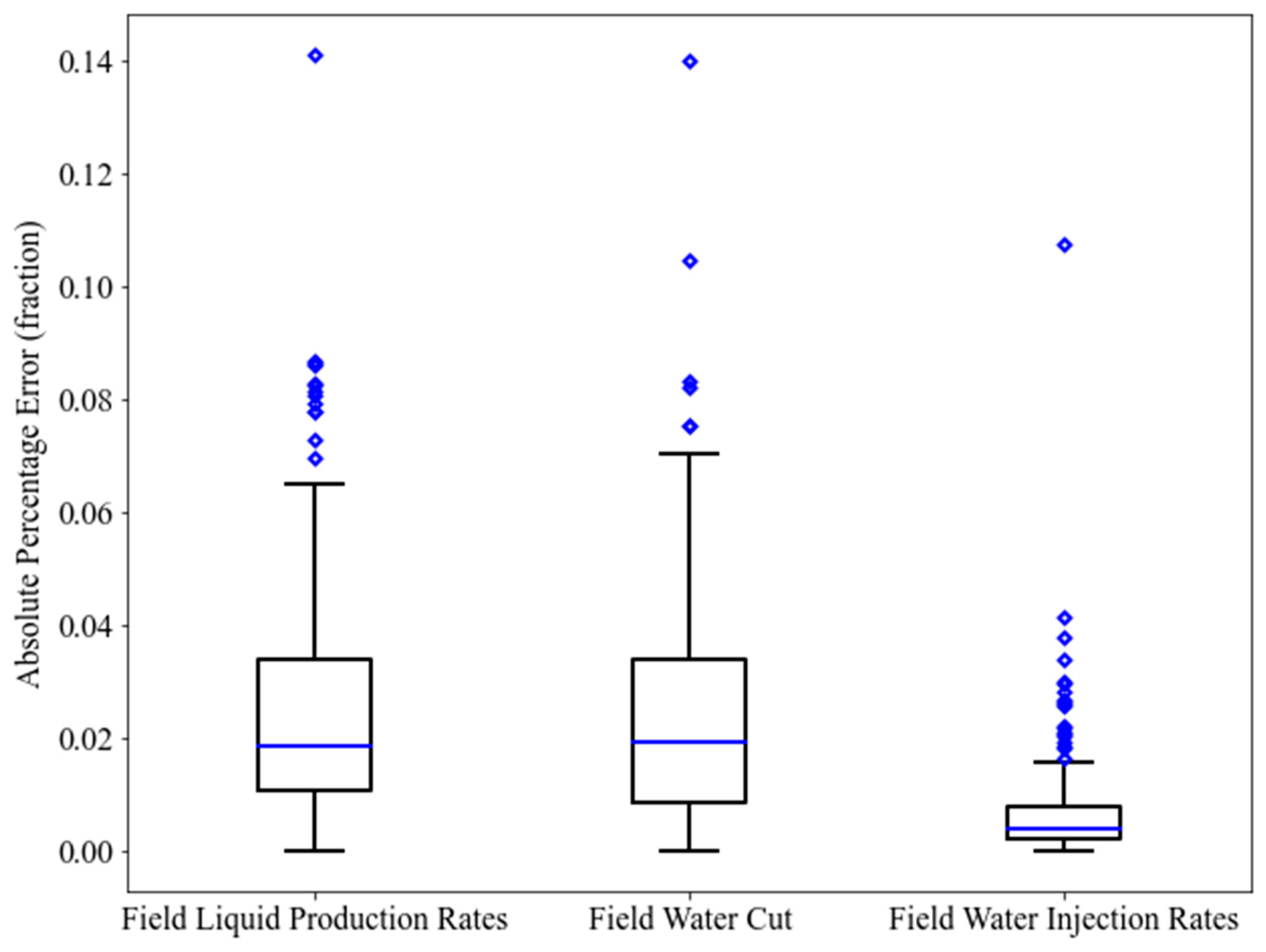
The MLP was chosen as the ML technique to develop the proxy models in this work. The proxy modeling was performed using the Scikit-Learn with the aid of Python programming language [33]. As explained in the workflow, there are two stages of proxy modeling. To assess the reliability of these proxy models, we implemented three statistical metrics, namely Coefficient of Determination (R2), Root Mean Squared Error (RMSE), and Average Absolute Percentage Error (AAPE). Different examples of statistical metrics in tandem with their formulations can be referred to in [34]. The training and testing results of the first stage of proxy modeling (global proxy modeling) are presented in Table 6. In addition, the boxplots of the Absolute Percentage Error (APE) for the training and testing data points are demonstrated in Figure 13 and Figure 14.
From the boxplots, it can be seen that MLP-FWIR displays the smallest range of APE as compared to MLP-FLPR and MLP-FWCT, in terms of training and testing. Furthermore, the statistics on R2 and AAPE provided in Table 6 also confirm the better performance of MLP-FWIR for training and testing. This better performance does not undermine the predictability of MLP-FLPR and MLP-FWCT. Numerous outliers are noticed in the boxplots for all the three models. Hence, the predictability of these models needs to be further justified by applying blind validation cases. To conduct this justification, ten blind validation cases were generated, as explained in Figure 12. The performance metrics of the proxy models for these blind validation cases are displayed in Table 7. The results consist of the mean of all the ten blind validation cases. It is observed that MLP-FWIR still outperforms the other two models. In MLP-FLPR, the mean R2, the mean RMSE, and the mean AAPE might be less satisfactory. From Table 6 and Table 7, it is worth noting that MLP-FLPR generally illustrates relatively poor performance. This could be due to the complexity of the reservoir model used. This implies that the database provided might not adequately reflect the physics of the reservoir. In MLP-FWCT too, a similar issue can be observed in terms of the AAPE. Despite this fact, these models are still considered practical to generate insightful optimal solutions for local proxy modeling.
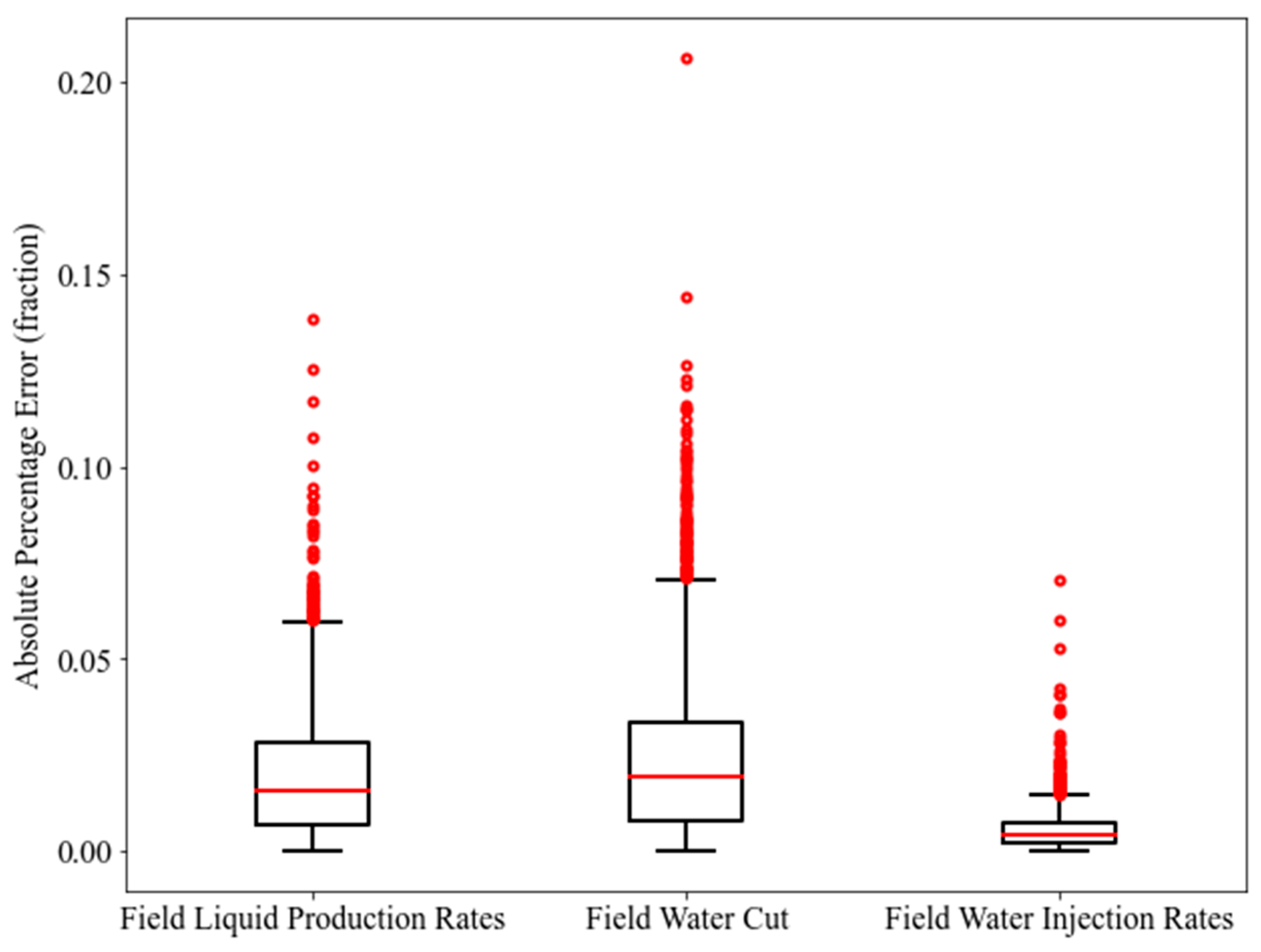
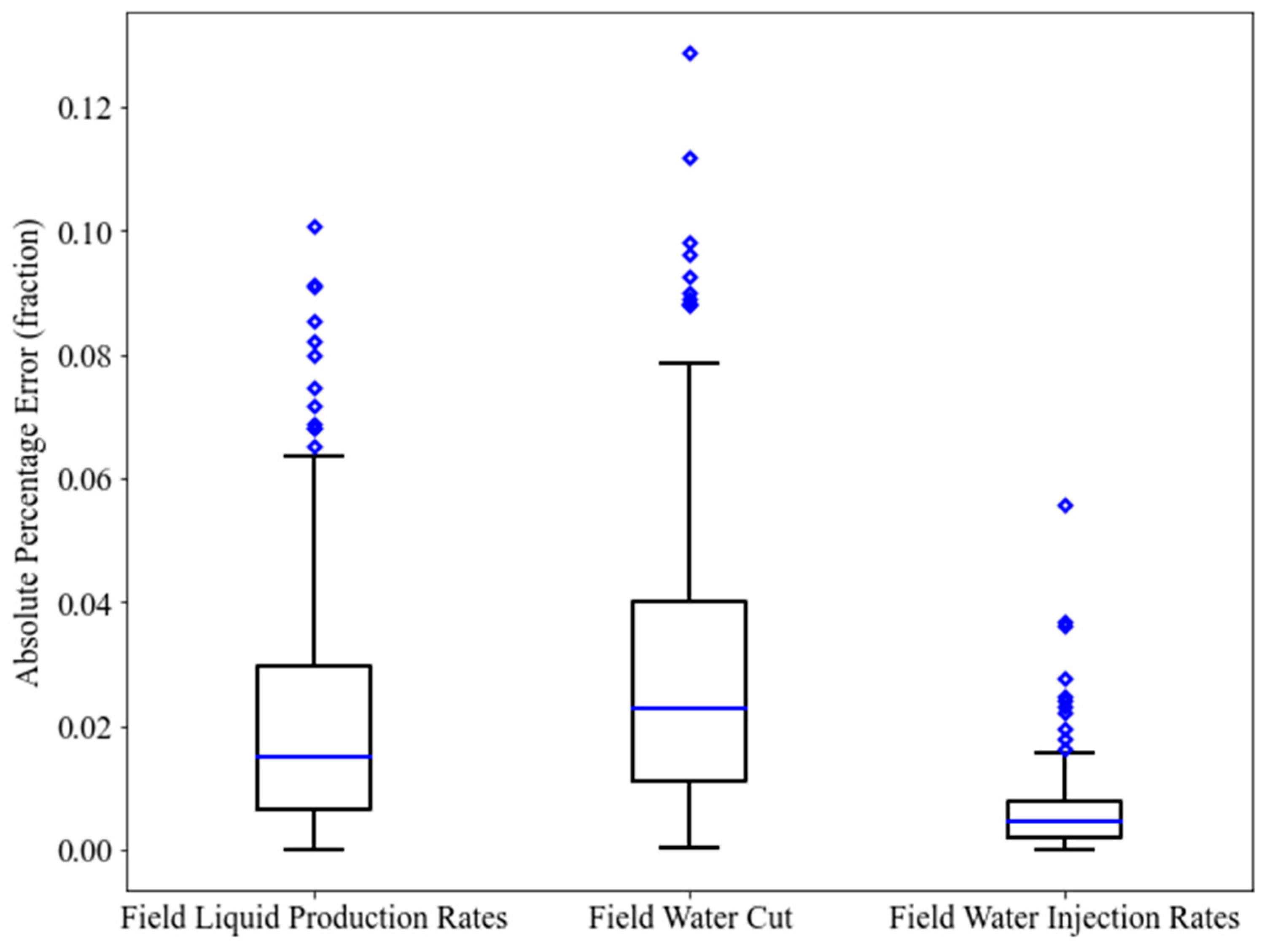
Upon completion of the first stage of proxy modeling, the proxy models are readily employed for optimization with the GA and the PSO. However, optimization at this phase aims at creating a “useful” database for the training of local proxy models. This database consists of the data that have a closer proximity to the “true” optimal solution. When the new “training” database is ready, it can be applied to establish the local proxy models. In this case, two different algorithms result in two different databases. It is anticipated that the performance metrics of the local proxy models demonstrated more improvement as compared with the global proxy models. For illustrative purposes, the corresponding boxplots of the APE in the training and testing phases are portrayed in Figure 15 and Figure 16 for GA as well as in Figure 17 and Figure 18 for PSO, respectively. For a more comprehensive evaluation, the training and testing results of the second stage of proxy modeling (local proxy modeling) are demonstrated in Table 8 for GA and Table 9 for PSO. The statistics in Table 8 and Table 9, highlight an improvement in terms of R2, RMSE, and AAPE as compared with the results from Table 6. This fulfills the goal of conducting the second stage of proxy modeling. In terms of blind validation, ten additional cases were created. The statistics displayed in Table 10 and Table 11 for blind validation, also show a good level of enhancement in the mean R2, the mean RMSE, and the mean AAPE as compared with those shown in Table 7.
One of the main goals of this work, which was achieving significant computational efficiency in tandem with good accuracy of results, was attained. For both the GA and the PSO algorithms, the framework (considering global and local proxy modeling as well as optimization) took about two days to complete. However, when the optimization was conducted with the reservoir simulator, both algorithms required about twelve days to finish. This demonstrates that the proposed framework can reduce the computational time by six times. It is essential to note that the framework runs the optimization 100 times in the case of global proxy modeling and 200 times for local proxy modeling. Nevertheless, the optimization with the reservoir simulator was only performed once. For this, the optimized NPVs obtained using the simulator coupled with GA and PSO are 6054.61 million USD and 5832.55 million USD, respectively.
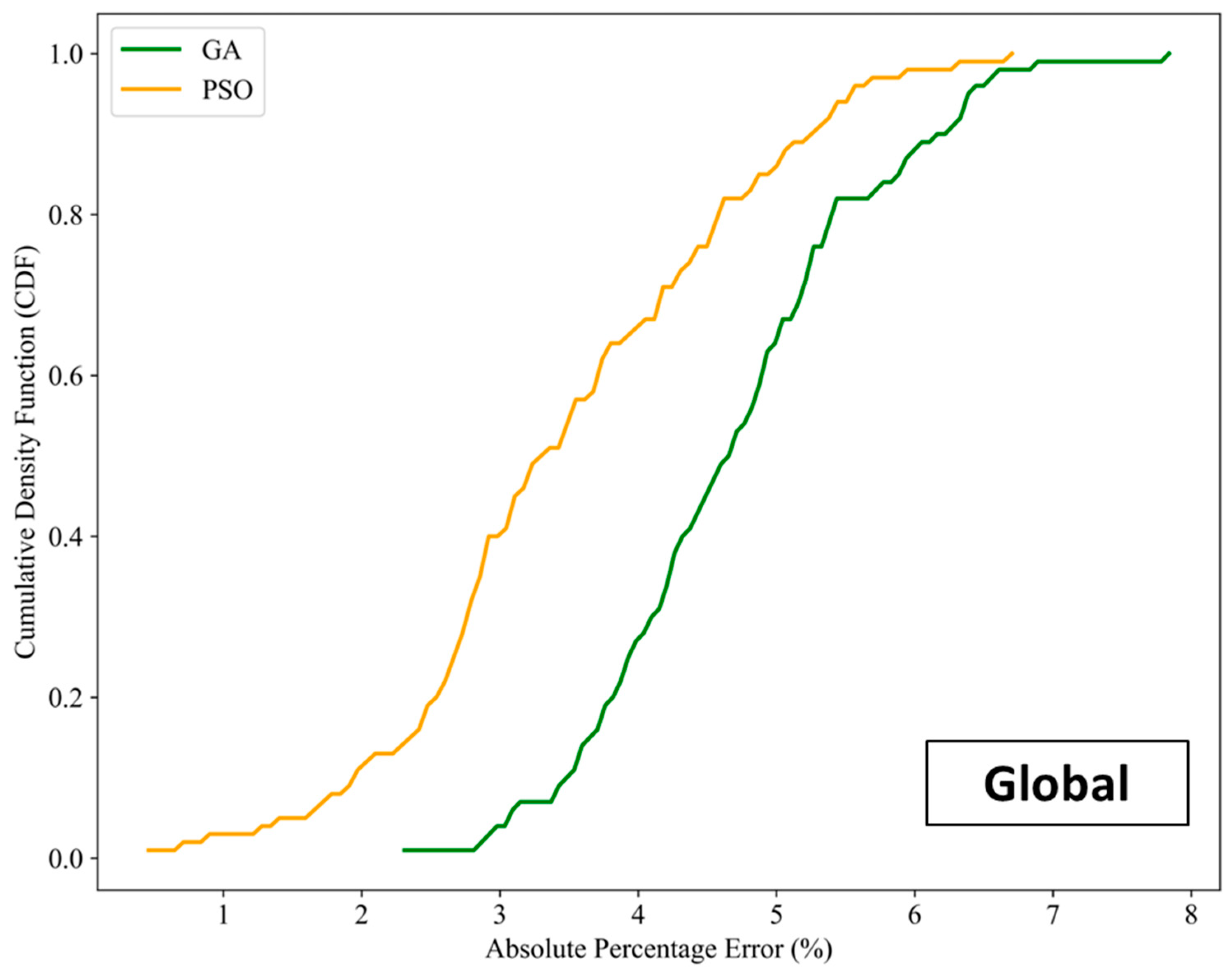
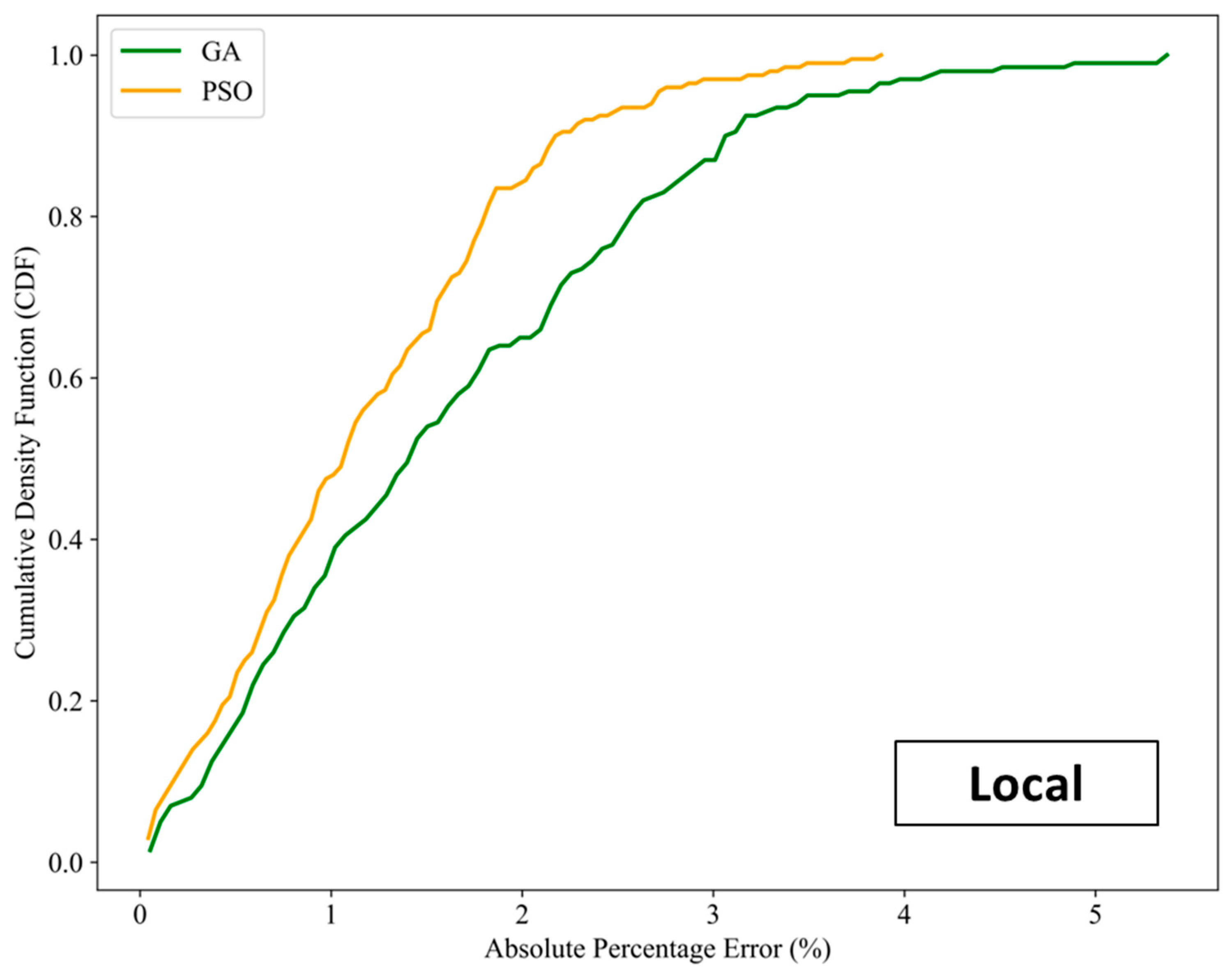
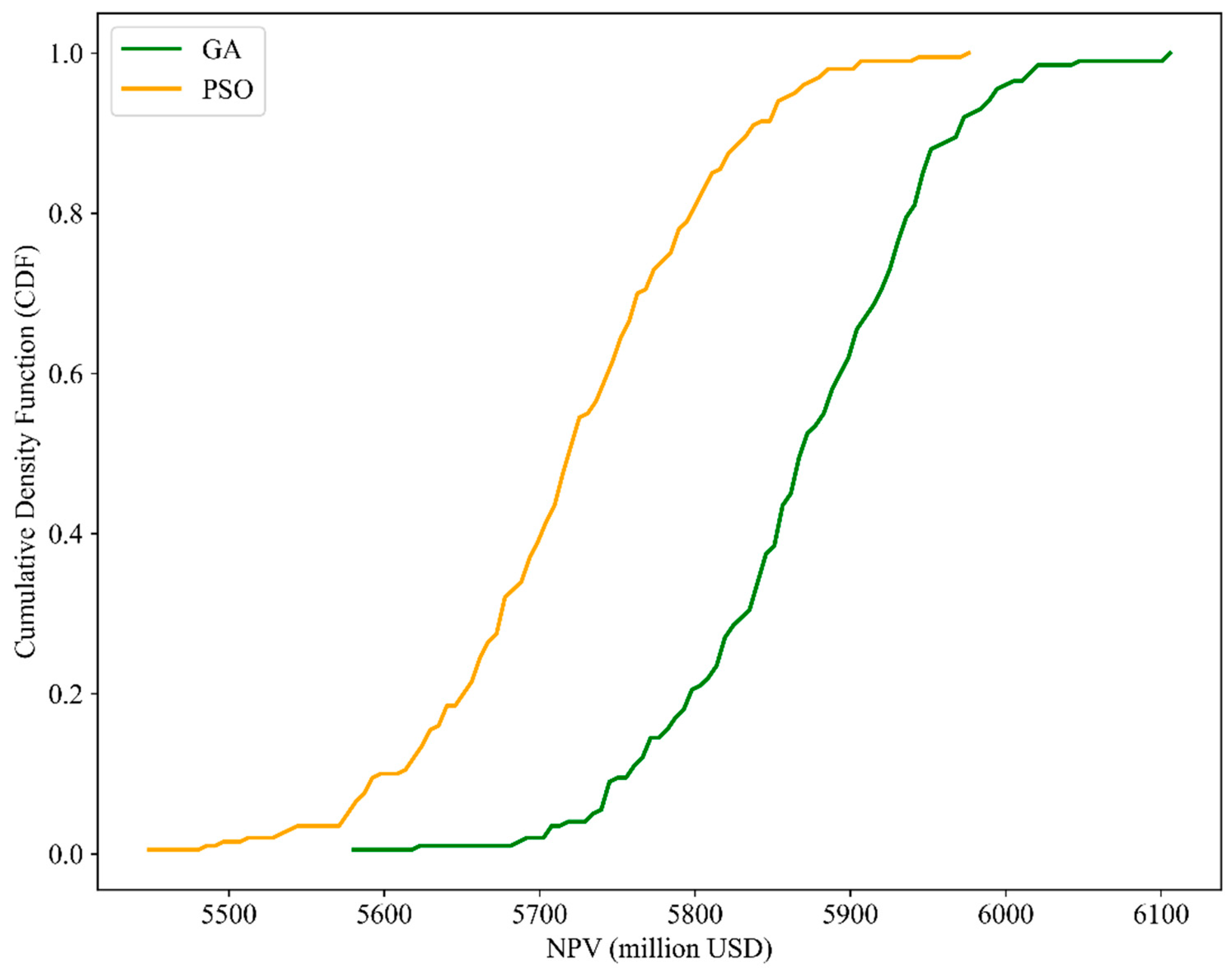
To further highlight the improvement of accuracy attained by conducting the two-stage proxy modeling, the cumulative density frequency (CDF) of absolute percentage error between the actual NPV and the NPV predicted by both global and local proxy models are plotted in Figure 19 and Figure 20, respectively. Due to the expensive computational demand of the reservoir simulator for the optimization task as explained above, the actual NPVs are calculated by feeding the optimized control variables obtained using the corresponding proxy model into the reservoir simulator. As the CDF plots display, the range of the APE yielded by local proxy models reduces as compared with that of global proxy models. Most of the resulting samples lie within the APE range of 0%–3% for both types of local proxy models. This verifies that local proxy modeling permits higher accuracy of optimal results. Additionally, proxy models coupled with PSO exhibit a higher chance of achieving results within a more desired level of accuracy (compared with GA). In terms of NPV calculation, the GA produces bigger values than the PSO. This is confirmed by the CDF plots of the NPVs in Figure 21, which show the actual NPVs obtained from the local proxy models.
The details highlighted in Figure 21 were obtained when the optimization was run 200 times. For each optimization run, there are 200 iterations. Thereafter, as explained previously, for each run, the resultant optimal control variables are fed into the reservoir simulator. This denotes that there will be 200 optimal NPV samples. With this, the highest NPV achieved (out of the 200 optimal solutions) is 6105.79 million USD for the GA. Using the respective control only in tandem with proxy models, the resulting NPV is 6131.79 million USD. In the case of the PSO, by feeding the 200 proxy-optimized solutions into the simulator, the highest NPV obtained is 5976.20 million USD. The computed NPV, by only employing proxy models, is 5854.37 million USD. The aforementioned scenario with the highest NPV of 5456.70 USD million was assumed to be the base case. By considering the NPVs obtained using the proxy models, it can be noticed that the GA resulted in an improvement of 12.4% (over the base case) whereas the PSO enhanced it by 7.29%. This shows that the optimality of the solution can be refined through the framework presented. Nonetheless, more studies need to be conducted to comprehensively discern if conducting further local proxy modeling enables a closer approximation to the “ground truth”.
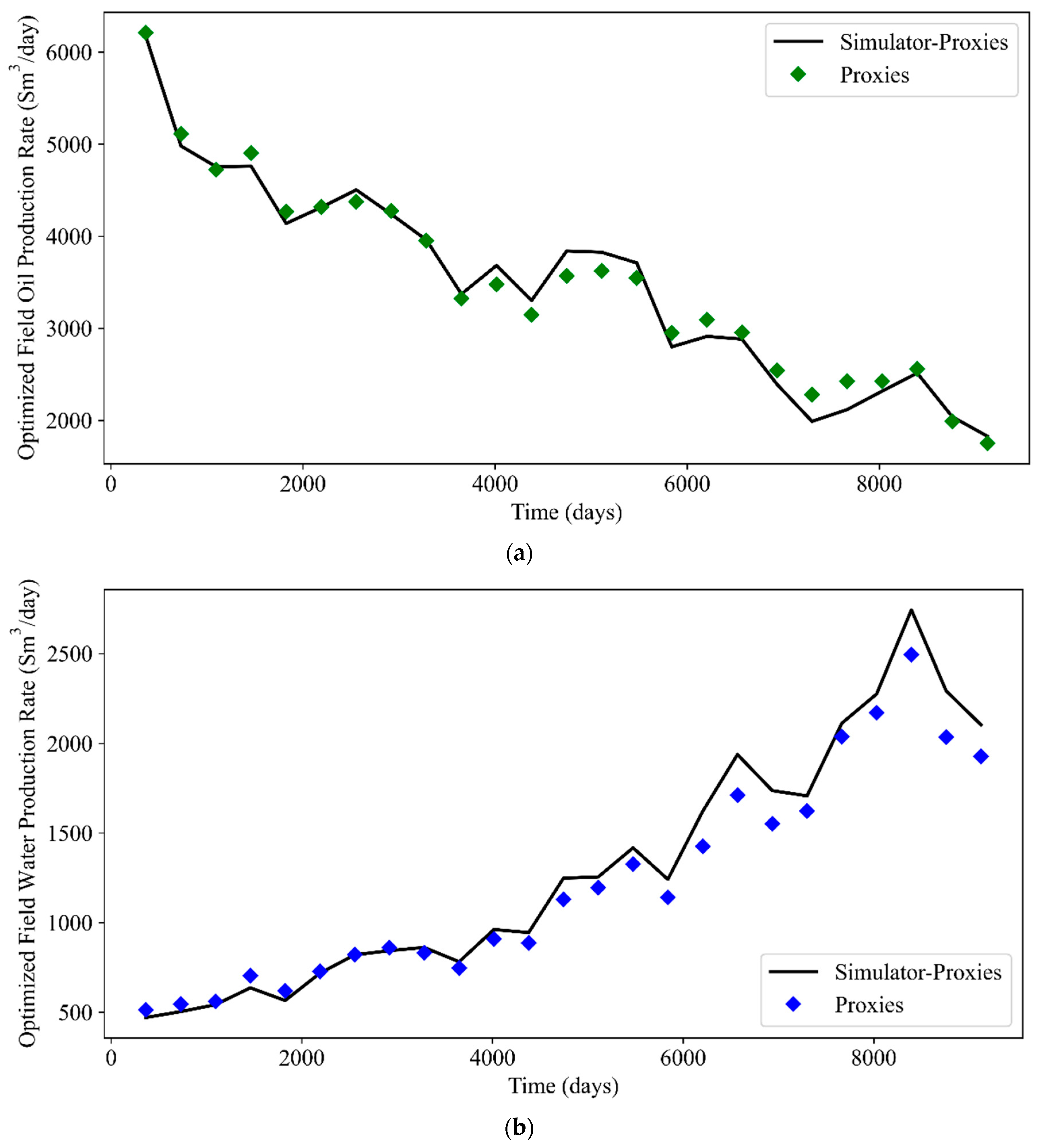
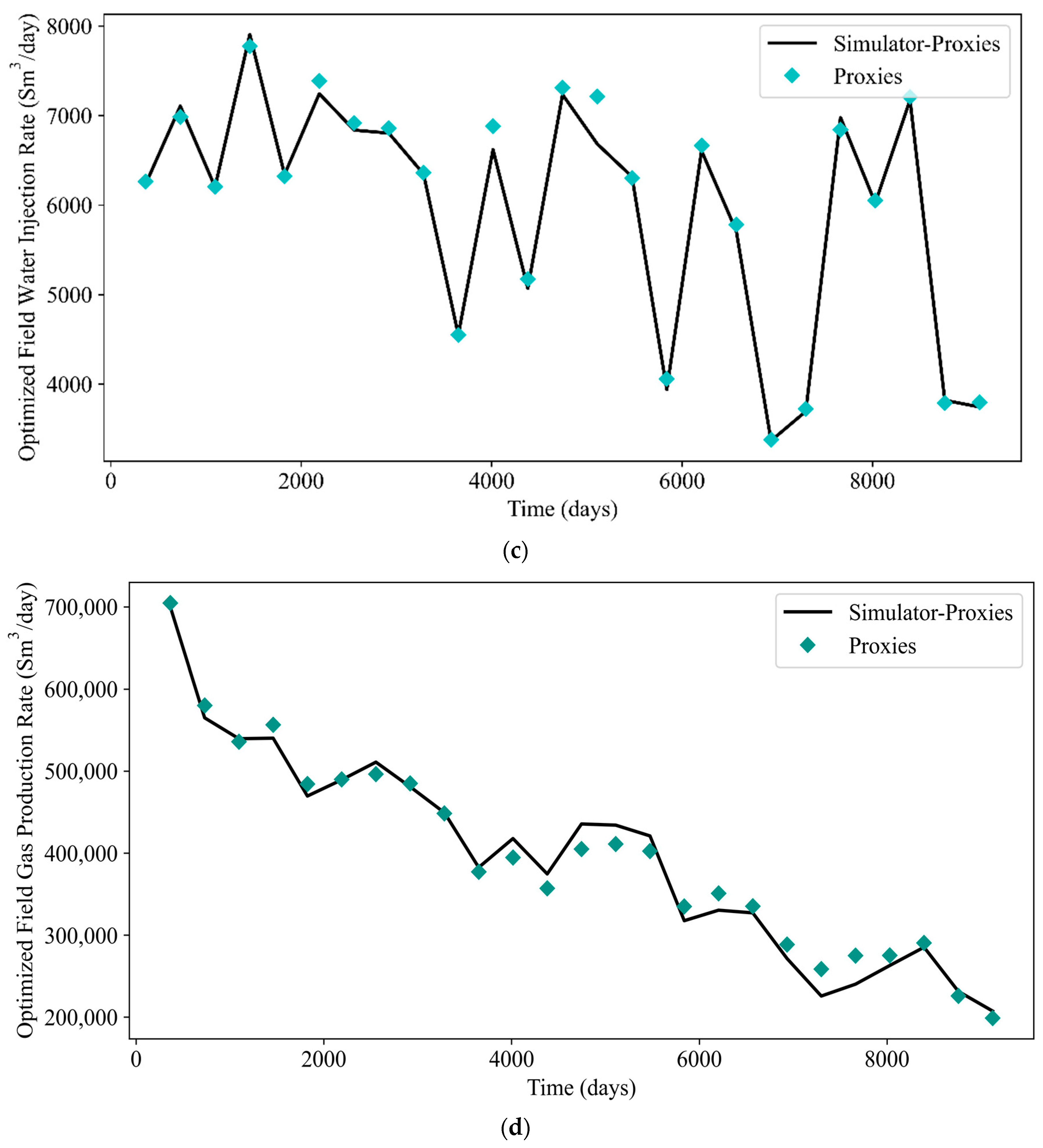
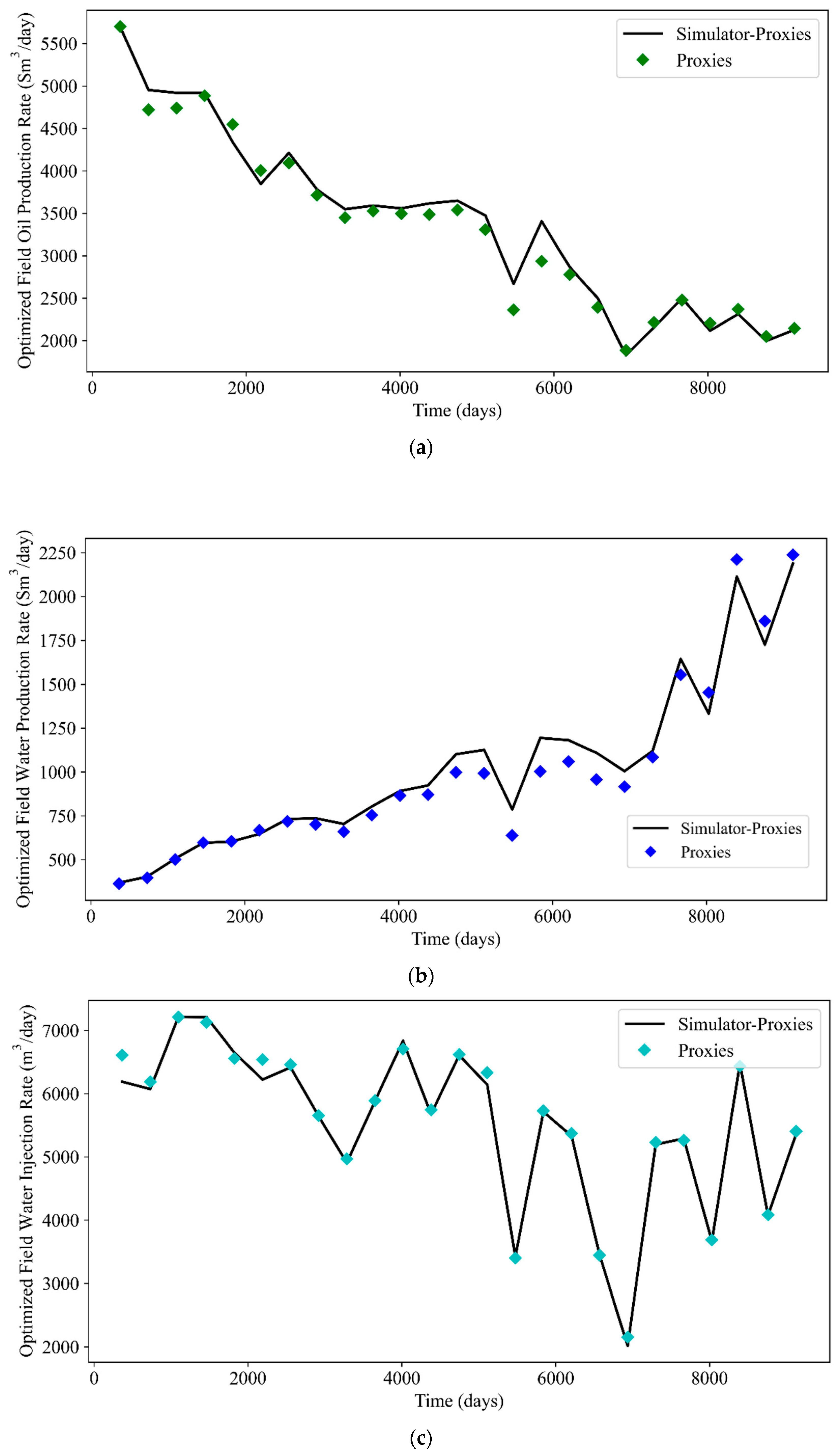
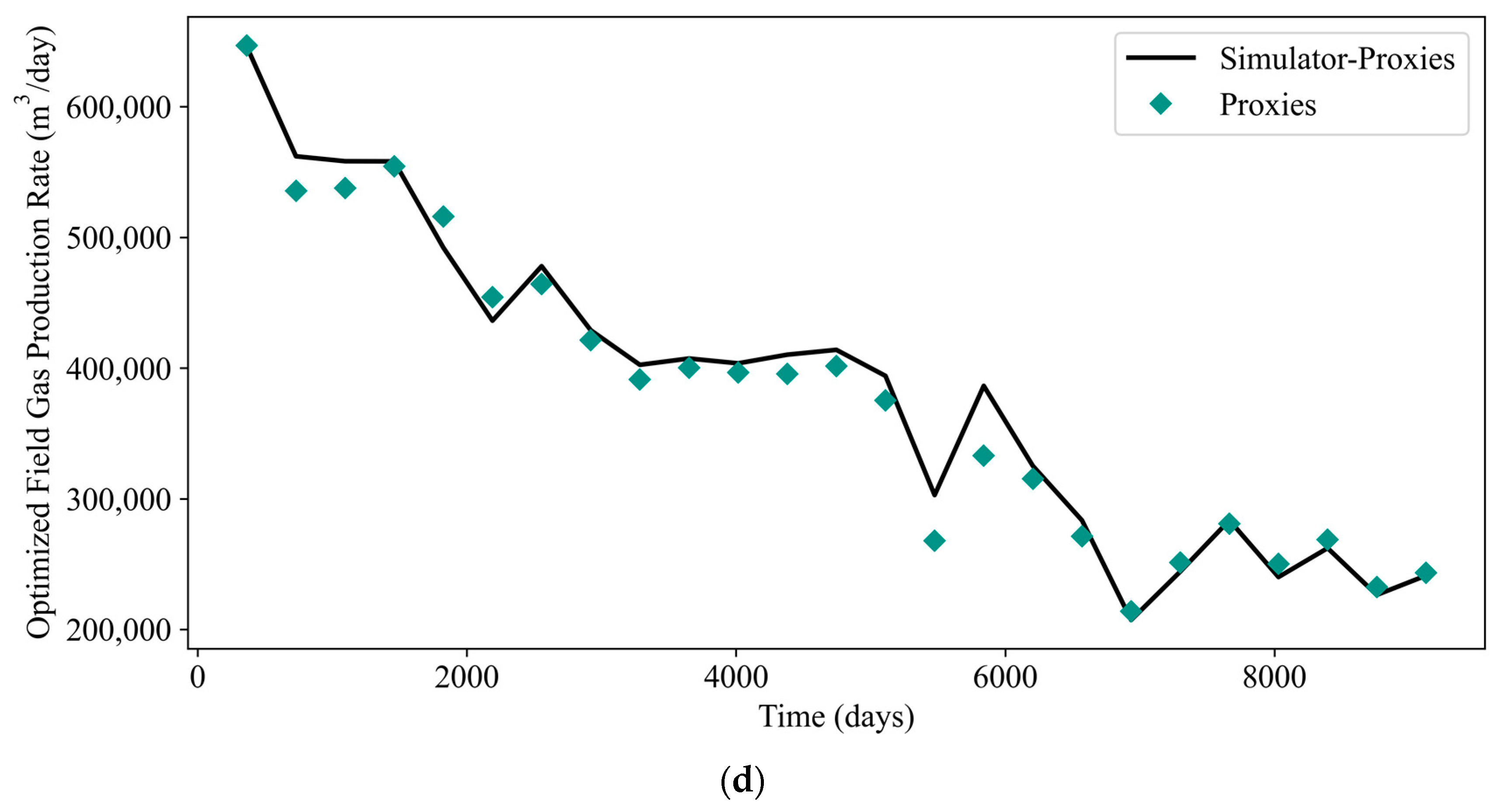
Plots of GA-optimized FOPR, FWPR, FWIR, and FGPR are shown in Figure 22. The corresponding metrics are tabulated in Table 12. PSO-optimized rates are shown in Figure 23 and the respective metrics are tabulated in Table 13. Based on these tables, it can be concluded that the values of RMSE and AAPE in general correspond less satisfactorily to the values of R2. This is reflected by the error estimation shown by several data points in both Figure 22 and Figure 23. Despite this fact, the proxy models still successfully capture the production profiles and serve their practical purposes. For illustration, only the cases with the highest NPV are shown in the plots. To avoid confusion, the term “simulator-proxies” refers to the results obtained from the reservoir simulator by implementing the optimal control produced by local proxy models. Based on these plots, the predictability of the local proxy models is further validated. The FOPR, FWPR, FWIR, and FGPR profiles obtained by the local proxy models generally match well with the profiles of simulator-proxies.
In general, the proposed framework has showcased good practical applications, considering the trade-off between accuracy and computational efficiency. Nonetheless, it is still subject to several limitations that are worth investigating further. The models developed from this framework are not “one-size-fits-all”. They are case-specific to serve the objective of the optimization problem under study. Furthermore, the proposed framework is yet to be verified in different optimization problems, such as well placement and choke optimization. This framework is limited to a geological realization and its maturity still needs to be justified considering geological uncertainty. Moreover, the proposed framework displays a good path to solving an optimization problem with 200 decision variables (a problem with a considerably high dimension). However, in terms of handling problems with even higher dimensionality, as reflected by most real-life applications, it is evident that several approaches can be integrated into this framework to reduce the pertinent dimension to increase its practicality. To the best of our knowledge, conducting production optimization with an efficiently reduced dimension of optimization variables, is still subject to extensive research. Regarding real-life applications, the proposed framework can also be extended to the paradigm of Top-Down Modeling [35] that only considers real field data to build the models.
Integrating another step of parameter optimization regarding both the structure of MLP and the variables of the nature-inspired algorithms will certainly be insightful. Attempting other advanced ML techniques, including Tree-based Pipeline Optimization Tool [36], can be researched to integrate the use of automated hyperparameter optimization in its workflow. In terms of solving a more sophisticated optimization problem, e.g., multi-objective optimization, the integration of NSGA-II (Non-dominated Sorting Genetic Algorithm II), suggested by Deb et al. [37], into the proposed framework can be considered. Some detailed studies are thus needed to achieve such enhancement by honoring the balance between computational speed and the accuracy of results predicted by the proxy models. Additionally, a combination of nature-inspired algorithms and derivative-based algorithms can also be studied and possibly used instead of only applying the nature-inspired algorithms. This has a good potential to improve the exploitation component of optimization as the exploration is taken care of by nature-inspired algorithms [38].
7. Conclusions
In this work, we have presented a framework of methodology that couples proxy models with derivative-free algorithms to conduct waterflooding optimization. The approach of proxy modeling has been modified by introducing two different stages, namely global and local proxy modeling. Global proxy models were developed using a database that was generated by employing the sampling technique and reservoir simulation. Upon developing the global proxy models, an optimization algorithm was employed with these models to create a new database. This new database was then applied to develop more refined proxy models (the local proxy models). We have selected MLP as the ML method to develop the proxy models. For each stage of proxy modeling, we built three models to predict the output of FLPR, FWCT, and FWIR at every timestep. These output values were then utilized to compute the NPV for optimization purposes. The optimization was performed using GA and PSO. It is important to note that FGPR is also involved in the computation of NPV. However, for the optimization problem, the profile of FGPR is similar to that of FOPR since the solution gas oil ratio, Rs, remains constant for the whole production period.
The results obtained suggest that the two-stage proxy modeling can improve optimal solution. Such improvement is noticeable in terms of training, testing, blind validation, and optimization. Additionally, the computational efficiency of this framework is higher than solely relying on the reservoir simulator for optimization. The accuracy of results is not sacrificed upon attaining such a higher computational efficiency. This signifies the benefit of this framework for practical purposes. The primary objective of the proposed framework has been accomplished, although there are several limitations associated with it, such as lack of generalization and consideration of geological uncertainty. Nonetheless, a rudimentary framework has been successfully developed here, and further improvements should be considered for more real-life and robust applications. Detailed studies, including identifying the impact of each step of the framework (such as training of models and optimization), are recommended to strive for higher maturity of its employment.
Author Contributions
C.S.W.N.: Conceptualization, Methodology, Software, Formal Analysis, Data Curation, Investigation, Writing—original draft, Writing—reviewing and editing, Visualization. A.J.G.: Methodology, Writing—reviewing and editing, Supervision. W.W.: Software, Data Curation, Writing—original draft, Writing—reviewing and editing, Visualization. All authors have read and agreed to the published version of the manuscript.
Funding
The APC was funded by Norwegian University of Science and Technology.
Data Availability Statement
Publicly available datasets were analyzed in this study. This data can be found here: https://www.unisim.cepetro.unicamp.br/benchmarks/br/unisim-i/unisim-i-d.
Acknowledgments
This research is a part of BRU21—NTNU Research and Innovation Program on Digital Automation Solutions for the Oil and Gas Industry (http://www.ntnu.edu/bru21 (accessed on 14 February 2023)).
Conflicts of Interest
The authors declare no conflict of interest.
References
- Russell, S.; Norvig, P. Artificial Intelligence A Modern Approach, 3rd ed.; Pearson: Hoboken, New Jersey, USA, 2010. [Google Scholar]
- Mohaghegh, S. Data-Driven Analytics for the Geological Storage of CO2; CRC Press: Boca Raton, FL, USA, 2018. [Google Scholar]
- Mohaghegh, S.D. Shale Analytics; Springer: Berlin/Heidelberg, Germany, 2017. [Google Scholar]
- Nwachukwu, A.; Jeong, H.; Pyrcz, M.; Lake, L.W. Fast Evaluation of Well Placements in Heterogeneous Reservoir Models Using Machine Learning. J. Pet. Sci. Eng. 2018, 163, 463–475. [Google Scholar] [CrossRef]
- Alakeely, A.; Horne, R.N. Simulating the Behavior of Reservoirs with Convolutional and Recurrent Neural Networks. SPE Reserv. Eval. Eng. 2020, 23, 992–1005. [Google Scholar] [CrossRef]
- Alakeely, A.; Horne, R. Simulating Oil and Water Production in Reservoirs with Generative Deep Learning. SPE Reserv. Eval. Eng. 2022, 25, 751–773. [Google Scholar] [CrossRef]
- Brundred, L.L.; Brudred, L.L., Jr. Economics of Water Flooding. J. Pet. Technol. 1955, 7, 12–17. [Google Scholar] [CrossRef]
- Ng, C.S.W.; Jahanbani Ghahfarokhi, A.; Nait Amar, M. Application of Nature-Inspired Algorithms and Artificial Neural Network in Waterflooding Well Control Optimization. J. Pet. Explor. Prod. Technol. 2021, 11, 3103–3127. [Google Scholar] [CrossRef]
- Ng, C.S.W.; Ghahfarokhi, A.J.; Nait Amar, M. Production Optimization under Waterflooding with Long Short-Term Memory and Metaheuristic Algorithm. Petroleum 2022, 9, 53–60. [Google Scholar] [CrossRef]
- Chen, G.; Zhang, K.; Zhang, L.; Xue, X.; Ji, D.; Yao, C.; Yao, J.; Yang, Y. Global and Local Surrogate-Model-Assisted Differential Evolution for Waterflooding Production Optimization. SPE J. 2020, 25, 105–118. [Google Scholar] [CrossRef]
- Chen, G.; Zhang, K.; Xue, X.; Zhang, L.; Yao, C.; Wang, J.; Yao, J. A Radial Basis Function Surrogate Model Assisted Evolutionary Algorithm for High-Dimensional Expensive Optimization Problems. Appl. Soft Comput. 2022, 116, 108353. [Google Scholar] [CrossRef]
- Yang, X.-S. Chapter 1—Introduction to Algorithms. In Nature-Inspired Optimization Algorithms; Yang, X.-S., Ed.; Elsevier: Oxford, UK, 2014; pp. 1–21. ISBN 978-0-12-416743-8. [Google Scholar]
- Nait Amar, M.; Jahanbani Ghahfarokhi, A.; Ng, C.S.W.; Zeraibi, N. Optimization of WAG in Real Geological Field Using Rigorous Soft Computing Techniques and Nature-Inspired Algorithms. J. Pet. Sci. Eng. 2021, 206, 109038. [Google Scholar] [CrossRef]
- Nait Amar, M.; Zeraibi, N.; Jahanbani Ghahfarokhi, A. Applying Hybrid Support Vector Regression and Genetic Algorithm to Water Alternating CO2 Gas EOR. Greenh. Gases Sci. Technol. 2020, 10, 613–630. [Google Scholar] [CrossRef]
- Ng, C.S.W.; Nait Amar, M.; Jahanbani Ghahfarokhi, A.; Imsland, L.S. A Survey on the Application of Machine Learning and Metaheuristic Algorithms for Intelligent Proxy Modeling in Reservoir Simulation. Comput. Chem. Eng. 2023, 170, 108107. [Google Scholar] [CrossRef]
- Nait Amar, M.; Zeraibi, N.; Redouane, K. Bottom Hole Pressure Estimation Using Hybridization Neural Networks and Grey Wolves Optimization. Petroleum 2018, 4, 419–429. [Google Scholar] [CrossRef]
- Ng, C.S.W.; Jahanbani Ghahfarokhi, A.; Nait Amar, M. Well Production Forecast in Volve Field: Application of Rigorous Machine Learning Techniques and Metaheuristic Algorithm. J. Pet. Sci. Eng. 2022, 208, 109468. [Google Scholar] [CrossRef]
- McKay, M.D.; Beckman, R.J.; Conover, W.J. A Comparison of Three Methods for Selecting Values of Input Variables in the Analysis of Output from a Computer Code. Technometrics 1979, 42, 55–61. [Google Scholar] [CrossRef]
- Avansi, G.D.; Schiozer, D.J. UNISIM-I: Synthetic Model for Reservoir Development and Management Applications. Int. J. Model. Simul. Pet. Ind. 2015, 9, 21–30. [Google Scholar]
- Ravenne, C.; Galli, A.; Doligez, B.; Beucher, H.; Eschard, R. Quantification of Facies Relationships via Proportion Curves. In Geostatistics Rio 2000, Proceedings of the Geostatistics Sessions of the 31 st International Geological Congress, Rio de Janeiro, Brazil, 6–17 August 2000; Springer: Dordrecht, The Netherlands, 2002. [Google Scholar]
- Gaspar, A.T.; Santos, A.; Maschio, C.; Avansi, G.; Filho, J.H.; Schiozer, D. Study Case for Reservoir Exploitation Strategy Selection Based on UNISIM-I Field; UNICAMP Universidade Estadual de Campinas: Campinas, Brazil, 2015. [Google Scholar]
- Deutsch, C. Calculating Effective Absolute Permeability in Sandstone/Shale Sequences. SPE Form. Eval. 1989, 4, 343–348. [Google Scholar] [CrossRef]
- Newman, G.H. Pore-volume compressibility of consolidated, friable, and unconsolidated reservoir rocks under hydrostatic loading. J. Pet. Technol. 1973, 25, 129–134. [Google Scholar] [CrossRef]
- Hall, H.N. Compressibility of Reservoir Rocks. J. Pet. Technol. 1953, 5, 17–19. [Google Scholar] [CrossRef]
- van der Knaap, W. Nonlinear Behavior of Elastic Porous Media. Trans. AIME 1959, 216, 179–187. [Google Scholar] [CrossRef]
- Holland, J.H. Genetic Algorithms. Sci. Am. 1992, 267, 66–73. [Google Scholar] [CrossRef]
- Lynch, M. Evolution of the Mutation Rate. Trends Genet. 2010, 26, 345–352. [Google Scholar] [CrossRef] [PubMed] [Green Version]
- Kennedy, J.; Eberhart, R. Particle Swarm Optimization. In Proceedings of the IEEE International Conference on Neural Networks, Perth, Australia, 27 November–1 December 1995. [Google Scholar]
- Buduma, N.; Locascio, N. Fundamentals of Deep Learning: Designing Next-Generation Machine Intelligence Algorithms; O’Reilly Media: Sebastopol, CA, USA, 2017; ISBN 9781491925614. [Google Scholar]
- Ng, C.S.W.; Jahanbani Ghahfarokhi, A. Adaptive Proxy-Based Robust Production Optimization with Multilayer Perceptron. Appl. Comput. Geosci. 2022, 16, 100103. [Google Scholar] [CrossRef]
- Kingma, D.P.; Ba, J.L. Adam: A Method for Stochastic Optimization. In Proceedings of the 3rd International Conference on Learning Representations, San Diego, CA, USA, 7–9 May 2015. [Google Scholar]
- Pedregosa, F.; Varoquaux, G.; Gramfort, A.; Michel, V.; Thirion, B.; Grisel, O.; Blondel, M.; Prettenhofer, P.; Weiss, R.; Dubourg, V.; et al. Scikit-Learn: Machine Learning in Python. J. Mach. Learn. Res. 2011, 12, 2825–2830. [Google Scholar]
- Van Rossum, G.; Drake, F.L. Python 3 Reference Manual; CreateSpace: Scotts Valley, CA, USA, 2009. [Google Scholar]
- Hemmati-Sarapardeh, A.; Larestani, A.; Nait Amar, M.; Hajirezaie, S. Applications of Artificial Intelligence Techniques in the Petroleum Industry; Gulf Professional Publishing: Houston, TX, USA, 2020. [Google Scholar]
- Mohaghegh, S.D. Data-Driven Reservoir Modeling; Society of Petroleum Engineers: Richardson, TX, USA, 2017; ISBN 9788578110796. [Google Scholar]
- Olson, R.S.; Moore, J.H. TPOT: A Tree-Based Pipeline Optimization Tool for Automating Machine Learning BT—Automated Machine Learning: Methods, Systems, Challenges. In Workshop on Automatic Machine Learning; Hutter, F., Kotthoff, L., Vanschoren, J., Eds.; Springer International Publishing: Cham, Switzerland, 2019; pp. 151–160. ISBN 978-3-030-05318-5. [Google Scholar]
- Deb, K.; Pratap, A.; Agarwal, S.; Meyarivan, T. A Fast and Elitist Multiobjective Genetic Algorithm: NSGA-II. IEEE Trans. Evol. Comput. 2002, 6, 182–197. [Google Scholar] [CrossRef] [Green Version]
- Alimo, S.R.; Beyhaghi, P.; Bewley, T.R. Optimization Combining Derivative-Free Global Exploration with Derivative-Based Local Refinement. In Proceedings of the 2017 IEEE 56th Annual Conference on Decision and Control (CDC), Melbourne, Australia, 12–15 December 2017; pp. 2531–2538. [Google Scholar]
Figure 1.
UNISIM-I-D NTG distribution: (a) Fine grid and (b) Upscaled model [19].
Figure 1.
UNISIM-I-D NTG distribution: (a) Fine grid and (b) Upscaled model [19].

Figure 2.
UNISIM-I-D upscaled porosity results.

Figure 3.
Porosity versus permeability: (a) Core analysis data [19] in which the blue dot refers to the core sample whereas the red line refers to the equation and (b) Upscaled model.
Figure 3.
Porosity versus permeability: (a) Core analysis data [19] in which the blue dot refers to the core sample whereas the red line refers to the equation and (b) Upscaled model.

Figure 4.
Upscaled permeability relationship in: (a) I-J direction; (b) I-K direction.

Figure 5.
Static properties used for simulation (a) Porosity, (b) Net-to-Gross, (c) Permeability I-direction, and (d) Permeability K-direction.
Figure 5.
Static properties used for simulation (a) Porosity, (b) Net-to-Gross, (c) Permeability I-direction, and (d) Permeability K-direction.

Figure 6.
Oil properties used for simulation.

Figure 7.
Gas properties used for simulation.

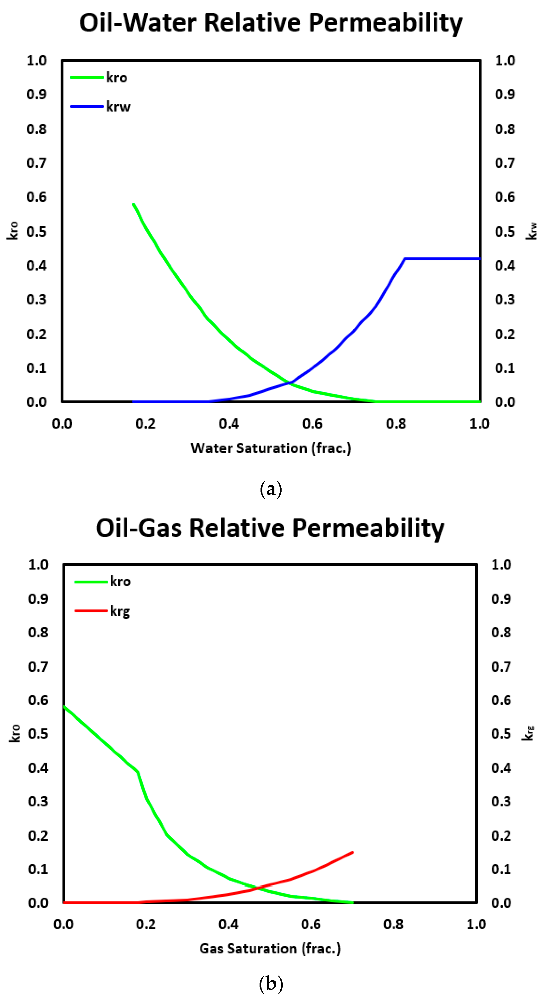
Figure 8.
Relative permeability (a) Oil-Water and (b) Oil-Gas.

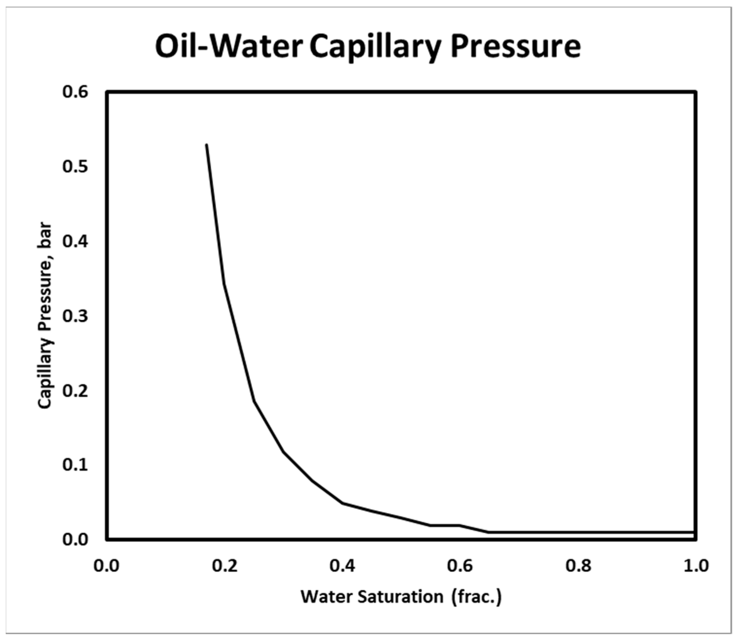
Figure 9.
Oil-water capillary pressure.

Figure 10.
Water-oil contact (WOC) definition: (a) Region definition (b) Distribution of initial fluid saturation.
Figure 10.
Water-oil contact (WOC) definition: (a) Region definition (b) Distribution of initial fluid saturation.

Figure 11.
Relationship between input parameters and output for the proxy models.

Figure 12.
Workflow of the proposed methodology.

Figure 13.
Boxplot of the Absolute Percentage Error of the training data points (global proxy modeling).
Figure 13.
Boxplot of the Absolute Percentage Error of the training data points (global proxy modeling).

Figure 14.
Boxplot of the Absolute Percentage Error of the testing data points (global proxy modeling).
Figure 14.
Boxplot of the Absolute Percentage Error of the testing data points (global proxy modeling).

Figure 15.
Boxplot of the Absolute Percentage Error of the training data points (local proxy modeling-GA).
Figure 15.
Boxplot of the Absolute Percentage Error of the training data points (local proxy modeling-GA).

Figure 16.
Boxplot of the Absolute Percentage Error of the testing data points (local proxy modeling-GA).
Figure 16.
Boxplot of the Absolute Percentage Error of the testing data points (local proxy modeling-GA).

Figure 17.
Boxplot of the Absolute Percentage Error of the training data points (local proxy modeling-PSO).
Figure 17.
Boxplot of the Absolute Percentage Error of the training data points (local proxy modeling-PSO).

Figure 18.
Boxplot of the Absolute Percentage Error of the testing data points (local proxy modeling-PSO).
Figure 18.
Boxplot of the Absolute Percentage Error of the testing data points (local proxy modeling-PSO).

Figure 19.
Cumulative Density Frequency plot of absolute percentage error between actual NPV and predicted NPV (global proxy modeling).
Figure 19.
Cumulative Density Frequency plot of absolute percentage error between actual NPV and predicted NPV (global proxy modeling).

Figure 20.
Cumulative Density Frequency plot of absolute percentage error between actual NPV and predicted NPV (local proxy modeling).
Figure 20.
Cumulative Density Frequency plot of absolute percentage error between actual NPV and predicted NPV (local proxy modeling).

Figure 21.
Cumulative Density Frequency plot of NPVs.

Figure 22.
Plots of GA-optimized rates: (a) FOPR, (b) FWPR, (c) FWIR, and (d) FGPR.


Figure 23.
Plots of PSO-optimized rates: (a) FOPR, (b) FWPR, (c) FWIR, and (d) FGPR.


Table 1.
Facies and Net to Gross rules.
| Facies | Net to Gross |
|---|---|
| 0 | 1.0 |
| 1 | 0.8 |
| 2 | 0.6 |
| 3 | 0.0 |
Table 2.
Water phase properties.
| Properties | Value |
|---|---|
| Reference pressure | 0.98067 bara |
| Water formation volume factor at reference pressure | 1.021 rm3/sm3 |
| Water compressibility | 4.8579 × 10⁻⁵ bar−1 |
| Water viscosity | 0.3 cP |
| Water viscosibility | 0 bar−1 |
Table 3.
Rock compressibility at reference pressure.
| Properties | Value |
|---|---|
| Rock compressibility | 5.4 × 10⁻⁵ bar−1 |
| Reference pressure | 315.77 bara |
Table 4.
Initial in-place volumes.
| Properties | Value |
|---|---|
| Initial Oil In Place | 130 MM Sm3 |
| Initial Dissolved Gas In Place | 14.7 B Sm3 |
Table 5.
Topology of the MLP.
| Type of Proxy Models | Number of Hidden Layers | Number of Hidden Nodes | Activation Functions (Hidden Layers) |
| FLPR | |||
| Global Proxy Model | 3 | 250 | ReLU |
| Local Proxy-GA | 3 | 250 | ReLU |
| Local Proxy-PSO | 3 | 200 | ReLU |
| Type of Proxy Models | Number of Hidden Layers | Number of Hidden Nodes | Activation Functions (Hidden Layers) |
| FWCT | |||
| Global Proxy Model | 3 | 150 | ReLU |
| Local Proxy-GA | 3 | 150 | ReLU |
| Local Proxy-PSO | 3 | 150 | ReLU |
| Type of Proxy Models | Number of Hidden Layers | Number of Hidden Nodes | Activation Functions (Hidden Layers) |
| FWIR | |||
| Global Proxy Model | 3 | 200 | ReLU |
| Local Proxy-GA | 3 | 200 | ReLU |
| Local Proxy-PSO | 3 | 200 | ReLU |
Table 6.
The training and testing results of global proxy modeling.
| Models (Training) | R2 | RMSE | AAPE |
| FLPR | 0.9510 | 150.06 | 3.357 |
| FWCT | 0.9933 | 0.0074 | 3.196 |
| FWIR | 0.9982 | 54.93 | 0.842 |
| Models (Training) | R2 | RMSE | AAPE |
| FLPR | 0.9516 | 153.01 | 3.440 |
| FWCT | 0.9920 | 0.0081 | 3.435 |
| FWIR | 0.9980 | 59.37 | 0.874 |
Table 7.
The blind validation results of global proxy modeling.
| Models (Blind Validation) | Mean R2 | Mean RMSE | Mean AAPE |
|---|---|---|---|
| FLPR | 0.9267 | 183.18 | 4.274 |
| FWCT | 0.9892 | 0.0092 | 4.075 |
| FWIR | 0.9974 | 64.03 | 1.169 |
Table 8.
The training and testing results of local proxy modeling (GA).
| Models (Training) | R2 | RMSE | AAPE |
| FLPR | 0.9660 | 108.69 | 1.959 |
| FWCT | 0.9961 | 0.0086 | 2.403 |
| FWIR | 0.9975 | 43.08 | 0.534 |
| Models (Testing) | R2 | RMSE | AAPE |
| FLPR | 0.9659 | 119.79 | 2.123 |
| FWCT | 0.9956 | 0.0094 | 2.774 |
| FWIR | 0.9978 | 46.51 | 0.588 |
Table 9.
The training and testing results of local proxy modeling (PSO).
| Models (Training) | R2 | RMSE | AAPE |
| FLPR | 0.9632 | 124.66 | 2.383 |
| FWCT | 0.9962 | 0.0076 | 2.276 |
| FWIR | 0.9974 | 52.09 | 0.620 |
| Models (Testing) | R2 | RMSE | AAPE |
| FLPR | 0.9630 | 128.53 | 2.442 |
| FWCT | 0.9953 | 0.0086 | 2.396 |
| FWIR | 0.9962 | 66.73 | 0.666 |
Table 10.
The blind validation results of local proxy modeling (PSO).
| Models (Blind Validation) | Mean R2 | Mean RMSE | Mean AAPE |
|---|---|---|---|
| FLPR | 0.9578 | 118.80 | 2.262 |
| FWCT | 0.9935 | 0.0105 | 3.037 |
| FWIR | 0.9975 | 42.46 | 0.581 |
Table 11.
The blind validation results of local proxy modeling (GA).
| Models (Blind Validation) | Mean R2 | Mean RMSE | Mean AAPE |
|---|---|---|---|
| FLPR | 0.9418 | 152.38 | 3.012 |
| FWCT | 0.9905 | 0.0112 | 3.155 |
| FWIR | 0.9971 | 51.76 | 0.681 |
Table 12.
Performance metrics of GA-optimized rates.
| Optimized Rate | R2 | RMSE | AAPE |
|---|---|---|---|
| FOPR | 0.9808 | 150.89 | 0.042 |
| FWPR | 0.9656 | 120.59 | 6.746 |
| FWIR | 0.9888 | 138.05 | 1.398 |
| FGPR | 0.9808 | 17,118.74 | 4.207 |
Table 13.
Performance metrics of PSO-optimized rates.
| Optimized Rate | R2 | RMSE | AAPE |
|---|---|---|---|
| FOPR | 0.9777 | 155.81 | 3.608 |
| FWPR | 0.9648 | 88.79 | 6.278 |
| FWIR | 0.9902 | 125.97 | 1.472 |
| FGPR | 0.9777 | 17,677.16 | 3.608 |
Disclaimer/Publisher’s Note: The statements, opinions and data contained in all publications are solely those of the individual author(s) and contributor(s) and not of MDPI and/or the editor(s). MDPI and/or the editor(s) disclaim responsibility for any injury to people or property resulting from any ideas, methods, instructions or products referred to in the content. |
© 2023 by the authors. Licensee MDPI, Basel, Switzerland. This article is an open access article distributed under the terms and conditions of the Creative Commons Attribution (CC BY) license (https://creativecommons.org/licenses/by/4.0/).
Share and Cite
MDPI and ACS Style
Ng, C.S.W.; Jahanbani Ghahfarokhi, A.; Wiranda, W. Fast Well Control Optimization with Two-Stage Proxy Modeling. Energies 2023, 16, 3269. https://0-doi-org.brum.beds.ac.uk/10.3390/en16073269
AMA Style
Ng CSW, Jahanbani Ghahfarokhi A, Wiranda W. Fast Well Control Optimization with Two-Stage Proxy Modeling. Energies. 2023; 16(7):3269. https://0-doi-org.brum.beds.ac.uk/10.3390/en16073269
Chicago/Turabian StyleNg, Cuthbert Shang Wui, Ashkan Jahanbani Ghahfarokhi, and Wilson Wiranda. 2023. "Fast Well Control Optimization with Two-Stage Proxy Modeling" Energies 16, no. 7: 3269. https://0-doi-org.brum.beds.ac.uk/10.3390/en16073269
Note that from the first issue of 2016, this journal uses article numbers instead of page numbers. See further details here.