A Novel Ensemble Model Based on an Advanced Optimization Algorithm for Wind Speed Forecasting

Abstract

Concerning the vision of achieving carbon neutral and peak carbon goals, wind energy is extremely important as a renewable and clean energy source. However, existing research ignores the implicit features of the data preprocessing technique and the role of the internal mechanism of the optimization algorithm, making it difficult to achieve high-accuracy prediction. To fill this gap, this study proposes a wind speed forecasting model that combines data denoising techniques, optimization algorithms, and machine learning algorithms. The model discusses the important parameters in the data decomposition technique, determines the best parameter values by comparing the model’s performance, and then decomposes and reconstructs the wind speed time series. In addition, a novel optimization algorithm is used to optimize the parameters of the machine learning algorithm using a waiting strategy and an aggressive strategy to improve the effectiveness of the model. Several control experiments were designed and implemented using 10-min wind speed data from three sites in Penglai, Shandong Province. Based on the numerical comparison results and the discussion of the proposed model, it is concluded that the developed model can obtain high accuracy and reliability of wind speed prediction in the short term relative to other comparative models and can have further applications in wind power plants.

1. Introduction

The use of fossil fuels on earth not only leads to an imbalance between energy supply and demand, but also increases the emission of harmful gases such as carbon dioxide and sulfur dioxide, causing environmental pollution problems [1]. Humans are actively exploring how to replace them with renewable and sustainable energy sources. Wind energy has become a highly publicized alternative to nonrenewable energy sources [2]. Furthermore, wind energy is receiving more and more attention because it is crucial for achieving carbon neutrality goals and transitioning to clean low-carbon energy [3]. However, the variability and intermittency of wind speed can lead to various issues, including damage and voltage problems in wind power generation systems [4]. Therefore, developing accurate wind speed prediction models is crucial for the energy sector. In past research, scholars have proposed various prediction models [5], which can be classified into physical models, standard statistical models, and artificial intelligence-based models.

The physical models are mainly based on numeric weather prediction (NWP) and usually consider physical properties such as temperature, pressure and density [6]. Pan et al. proposed a method for solving the probability prediction problem in the wind speed domain, which is a hybrid NWP combining current and future predicted numerical weather time series [7]. Zhao et al.’s optimized NWP data are used to forecast wind speed for the coming day [8]. Although the short-term prediction result of the NMP model is poor, it has strong long-term prediction ability [9].

The statistical model makes full use of historical and future data to obtain forecasting results [10], such as the autoregressive moving average (ARMA) [11], autoregressive integrated moving average (ARIMA) [12], and the Kalman filter (KF) [13]. Lydia et al. proposed two types of the AR model to solve the ten-minute and one-hour ahead wing speed forecasting shortcoming [14]. In North Dakota, a part of ARIMA was established to deal with one-day and two-day advance wind speed forecasting problems [15]. Liu et al. proposed a seasonal ARIMA model to apply to the offshore wind speed forecasting [16]. However, the wind speed time series has nonlinear characteristics, and statistical models are constrained by linear assumptions [17], making it difficult to capture suitable forecasting models.

Artificial intelligence methods have been used to capture nonlinear features to overcome the limitations of statistical models [18]. Many researchers have started to apply these methods for wind speed prediction. By using large amounts of historical data for training, AI methods can effectively adapt to the complex nonlinearity and uncertainty of wind speed time series [19]. Artificial intelligence (AI) methods have become the dominant and superior wind speed prediction models and are classified into three types: single models, hybrid models, and integrated models.

Common AI methods include artificial neural networks (ANN) [20], extreme learning machines (ELM) [21], and the support vector machine (SVM) [22]. With the development of neural networks, many neural networks with special structures have also been applied to wind speed prediction [23], such as the adaptive wavelet neural network [24], Emmanuel neural network (ENN) [21], and long and short term memory network (LSTM) [25]. Although a single model outperforms physical and statistical models, wind speed predictions from a single model are poor due to inherent drawbacks and the complex fluctuations in wind speed data, where linear and nonlinear features are always present in the data [26].

The hybrid model can repair the defects of the single model and further improve the forecasting model by combining the single model with an optimization algorithm [27]. Wang et al. proposed to tune the parameters in the support vector machine using the cuckoo search and genetic algorithm to improve the predictive performance of the model [28]. Research data preprocessing techniques such as integrated empirical mode decomposition (EEMD) [29], variational mode decomposition (VMD), and singular spectral analysis (SSA) [30] apply them to wind speed forecasting to improve the forecasting results of the model. In [31], an improved atomic search optimization algorithm (IASO) was used to search the extreme learning machine (ELM) to improve the wind speed prediction performance of the basic version. Fu et al. combined a Volterra series model with the VMD method to improve the beetle antenna search-based optimization algorithm and develop a new hybrid wind speed forecasting method [32].

Due to the high correlation between hybrid models and the performance of a single model, it is difficult for hybrid models to handle different time series, while ensemble models have advantages in time series forecasting [33]. Therefore, ensemble models have become the main method of wind speed forecasting. Wang et al. proposed an integration method consisting of an ANN, multi-objective bat algorithm (MOBA), and SSA to forecast wind speed [34]. Altan et al. proposed optimizing LSTM networks for wind speed prediction based on the GWO algorithm, and the results showed that optimizing LSTM using the GWO algorithm can be very competitive [35]. Wang et al. proposed an integrated model comprising CEEMD, ENN, and a multi-objective whale optimization algorithm (MOWOA) to predict short-term wind speeds [36]. Liu et al. proposed a wind speed forecasting ensemble system based on a data decomposition method, optimal subsequence predictor, and ensemble technology through multi-objective optimization [37]. Yang et al. adopted an integrated forecasting model based on decomposition technology and an optimization algorithm for integrating subsequence forecasting results, which has become an effective and promising method [38].

Based on the above analysis, a new ensemble forecast model is developed in this paper in order to achieve higher forecast accuracy. Firstly, the best model is determined by the comparison of single models. Secondly, the original wind speed series are decomposed and reconstructed by using data preprocessing techniques, and the single model is optimized by using the egret population optimization algorithm to set the parameters in the appropriate threshold range and continuously update and iterate to achieve a more accurate optimization effect and then make wind speed forecasts.

The main contributions of this paper are as follows: Firstly, the number of decomposition layers in the variational modal decomposition technique is discussed, and the optimal parameter values are determined by comparing the model performance, so that the original wind speed time series can be decomposed, denoised, and reconstructed, effectively improving the forecast accuracy of the model. Secondly, the definition domain of the parameters of the egret population optimization algorithm is discussed, and the best definition domain is determined by setting different definition domains for forecasting; then, the support vector machine is optimized, and the optimized support vector machine is further used to forecast the wind speed time series. The prediction accuracy is improved; in addition, the proposed innovative integrated model is trained and tested based on wind speed data from several sites of a large wind farm, and the results show that the model outperforms the traditional model. Therefore, the model can be applied to wind speed prediction in wind power plants.

The research content of this article is as follows: the second section introduces the methods used in the model; the third section mainly introduces the test criterion; the fourth section introduces data processing and analysis; the fifth section discusses the number of layers of VMD, the definition domain of the egret population optimization algorithm, and the DM test; and the sixth section is a summary.

2. Methodology

The methodology mainly contains an advanced data decomposition method, new optimization algorithm, and the mentioned ensemble model.

2.1. Variational Mode Decomposition (VMD) Technique

During decomposition, VMD requires a minimum sum of the estimated bandwidths for each modality. It is constrained by the fact that the sum of the decomposed modes is equal to the original signal. Then, the corresponding constraint variational problem is represented as

$$\left\{\begin{array}{c}\underset{\left\{v_k\right\},\left\{{\omega }_k\right\}}{min}\left\{{{\displaystyle \sum _{k=1}^k‖{\partial }_t\left[\left(\delta (t)+\frac{j}{\pi t}\right)\ast v_k(t)\right]\ast e^{-j{\omega }_{k}t}‖}}_2^2\right\}\\ s.t.{\displaystyle \sum _{k=1}^k{v}_k=f(t)}\end{array}\right.$$

(1)

where $f(t)$ represents the initial signal, $v_k$ is all the modals, k is the number of modal decomposition layers, t is the time, j is an imaginary number, ${\omega }_k$ is the center frequency of the kth component, and δ(t) is the Dirac distribution.

Lagrange multipliers are usually used to solve constrained problems. Therefore, in variational problems, the weights can be implemented using augmented Lagrange quantities to achieve better convergence and finiteness. Assuming no constrained problems, the VMD algorithm embeds quadratic penalties and Lagrange multipliers into the optimization process to ensure a constrained strictly conditional environment using the following extended expressions, which in turn transforms the optimization problem mentioned above into an unconstrained problem.

$$\begin{array}{l}L(\{v_k\},\{w_k\},\lambda )=\alpha {\displaystyle \sum _{k=1}^K{‖{\partial }_t\left[(\delta (t)+\frac{j}{\pi t})\ast v_k(t)\right]e^{-j{w}_{k}t}‖}_2^2}\\ +{‖f(t)-{\displaystyle \sum _k{v}_k(t)}‖}_2^2+〈\lambda (t),f(t)-{\displaystyle \sum _{k=1}^K{v}_k(t)}〉\\ \end{array}$$

(2)

where α represents the secondary penalty factor that reduces Gaussian noise interference, and λ is the Lagrange multiplier. The variational problem described above is solved using the alternating direction multiplier method (ADMM), and the optimization of the unconstrained problem can be expressed as

$${\widehat{v}}_k^{n+1}(\omega )=\frac{\widehat{f}(w)-{\displaystyle \sum _{j\ne k}{\widehat{v}}_j(\omega )+\frac{\widehat{\lambda }(\omega )}{2}}}{1+2\alpha {(\omega -{\omega }_k)}^2}$$

(3)

$${\omega }_k^{n+1}=\frac{{\displaystyle \int {}_0^{\infty }\omega {\left|{\widehat{v}}_k(\omega )\right|}^{2}d\omega }}{{\displaystyle \int {}_0^{\infty }{\left|{\widehat{v}}_k(\omega )\right|}^{2}d\omega }}$$

(4)

where ${\widehat{v}}_k^{n+1}(\omega )$ represents the Wiener filter of $\widehat{f}(w)-{\displaystyle \sum _{j\ne k}{\widehat{v}}_j(\omega )}$, and ${\omega }_k^{n+1}$ indicates the center of gravity of the power spectrum of the mode function.

2.2. Support Vector Machine

Support vector machines are usually used for data regression prediction. When dealing with nonlinear problems, kernel functions can be introduced. To simplify the processing of nonlinear problems, low-dimensional problems can be transformed into high-dimensional linear problems, which are applicable to complex signal problems. Gaussian radial basis function is a kernel function with strong localization ability, which can map samples to high-dimensional space, with wide application, better performance, and less parameters compared with other kernel functions.

$$K(x,y)=\exp (-\frac{{‖x-y‖}^2}{2{\sigma }^2})$$

(5)

where $\sigma$ is the width of kernel function. The optimization problem is transformed into the following equation:

$$\begin{gathered} \min {\displaystyle \sum _{i,j=1}^n({\beta }_i-{\beta }_i^{*})(}{\beta }_j-{\beta }_j^{*})K(x_i,x_j)+\epsilon {\displaystyle \sum _{i=1}^n({\beta }_i+{\beta }_i^{*})}-{\displaystyle \sum _{i=1}^n{y}_i({\beta }_i-{\beta }_i^{*})}s.t.{\displaystyle \sum _{i=1}^n({\beta }_i-{\beta }_i^{*})=0} \\ 0\le {\beta }_i,{\beta }_i^{*}\le D \end{gathered}$$

(6)

where D is penalty factor. The most optimal nonlinear regression function can be obtained.

$$f(x)={\displaystyle \sum _{i=1}^n({\beta }_i-{\beta }_i^{*})K(x_i}-x)+b$$

(7)

2.3. Egret Swarm Optimization Algorithm

The egret population optimization algorithm has development, exploration, comprehensive performance, stability, and convergence, in addition to the excellent performance and robustness of the ESOA algorithm in typical optimization applications [39]. ESOA consists of three main components: The sit-and-wait strategy, the aggressive strategy, and the discrimination condition. Each egret group is composed of n egret teams, with each team consisting of three egrets. Egret A uses the waiting strategy, while Egret B and Egret C use the random walk and surrounding mechanism of the aggressive strategy, respectively.

(1)

Sit and wait strategy:

The observation equation of the ${\hat{\mathrm{y}}}_{\mathrm{j}}=B(x_j)$, $y_j$ is the true fitness obtained at each iteration, the pseudo-gradient $g_j$ is the weight in the observation equation. The update location for egret A is as follows:

$$X_{a,j}=x_j+exp(-n/(0.1\ast n_{max}))\ast 0.1\ast hop\ast g_j$$

(8)

where n is the current iteration number; $n_{max}$ is the maximum number of iterations and hop is the range of feasible domains for arguments.

(2)

Aggressive strategies: Egret B is a random walk, and then updated as follows:

$$X_{b,j}=x_j+\frac{tan(r_{b,j})\ast hop}{1+n}$$

(9)

$r_{b,j}$ is the random number between $(-\frac{\pi }{2},\frac{\pi }{2})$.

Egret C is an encirclement strategy, and the updated location is as follows:

$$D_h=x_{jbest}-x_j$$

(10)

$$D_g=x_{gbest}-x_j$$

(11)

$$x_{c,j}=(1-r_j-r_h)\ast x_j+r_h\ast D_h+r_g\ast D_g$$

(12)

where $x_{jbest}$ and $x_{gbest}$ are the optimal values for egret teams and egret populations, respectively; $r_h$ and $r_g$ are random numbers between (0, 1).

(3)

Discrimination condition: After each egret in the egret squad calculates the updated position, it will jointly decide the update position of the egret squad, in the form below:

$$x_{s,j}=[x_{a,j},x_{b,j},x_{c,j}]$$

(13)

$$y_{s,j}=[y_{a,j},y_{b,j},y_{c,j}]$$

(14)

$$c_j=\arg \min (y_{s,j})$$

(15)

$$x_i=\left\{\begin{array}{l}{x}_{s,i/c_j} if y_{s,j}\left|{}_{c_j}<y_j or r<0.3\right.\\ x_j else\end{array}\right.$$

(16)

If $y_{s,j\left|c_j\right.}<y_j$, the egret squad chose to accept this option. Or if the random number r ∈ (0, 1) is less than 0.3, this means that there is a 30% chance of accepting a worse plan.

2.4. Data Feature Analysis Method

In most cases, developing a forecasting model involves computationally large complexity; so, in this article, we develop a suitable multiscale model to measure the complexity of the input data.

The Lempel–Ziv method measures the complexity characteristics of a time series. The smaller the Lempel–Ziv value of the sequence, the lower the complexity of the sequence, which means that the sequence contains more periodic components, stronger regularity, and less implicit frequency information. On the contrary, the larger the Lempel–Ziv value of the sequence, the higher the complexity, the worse the regularity of the feature, and the higher the frequency of the sequence. This article uses Lempel–Ziv algorithm to measure the complexity of the pattern, thereby improving the performance of the forecasting model.

To measure the complexity of Lempel–Ziv, it is necessary to convert the data series into a symbol sequence by comparing the data with a threshold, replacing a specific piece of data with 0 if the sequence is less than the threshold, otherwise replacing it with 1, and then analyzing the symbol sequence by identifying different quantities. When using the VMD method, applying the Lempel–Ziv method to identify the components, it is possible to select the optimal model for each component.

2.5. The Proposed Multiscale for Wind Power System

We propose a hybrid model framework, as shown in Figure 1, which is mainly composed of data decomposition technology, single model prediction, and an intelligent optimization algorithm.

Stage 1: The original wind speed time series is decomposed using variational model decomposition technology to remove noise and random fluctuations, thus decomposing into a set of IMF. To distinguish these components, the Lempel–Ziv algorithm is used to calculate the complexity of these components, and each component is predicted based on the identified data features.

Stage 2: Forecasting of single models. For single model prediction, ELM, ENN, naïve, and SVM with high accuracy are used as single models for prediction in this study to build the developed combined model. Therefore, the results of single model prediction are shown in Figure 1.

Stage 3: Determine the optimal weight coefficient for the forecasting model. Egret population optimization algorithm is used to continuously iteratively optimize the preprocessed data until the maximum number of iterations is reached, and the SVM of a single model is predicted according to the obtained model weight coefficient, so as to obtain the final prediction result.

Stage 4: Considering the complex seasonality of wind speed, this study selected four quarters of data to verify that the established model can solve the problem of wind speed prediction in different seasons. By comparing the data from four quarters with different models, the superiority of the developed model compared to the comparative model is demonstrated from different perspectives.

3. Test Criterion

3.1. The Performance Metric

In order to verify the superiority of the VMD-ESOA-SVM model more clearly and accurately, the average absolute and percentage error (MAPE), root mean square error (MAE), mean squared error (MSE), and average absolute scale error (MASE) were used to quantitatively determine the model’s performance. These performance metrics are calculated using the following equation:

$$\mathrm{MAPE}=\frac{1}{n}{\displaystyle \sum _{k=1}^n\left|\frac{y_k{}_{-}{\widehat{y}}_k}{y_k}\right|}\times 100\%$$

(17)

$$\mathrm{MAE}=\frac{1}{n}{\displaystyle \sum _{k=1}^n\left|{\widehat{y}}_k-y_k\right|}$$

(18)

$$\mathrm{MSE}=\frac{1}{\mathrm{n}}{\displaystyle \sum _{\mathrm{k}=1}^{\mathrm{n}}({\widehat{\mathrm{y}}}_{\mathrm{k}}-{\mathrm{y}}_{\mathrm{k}}}{)}^2$$

(19)

$$\mathrm{RMSE}=\sqrt{\left(\frac{1}{\mathrm{n}}{\displaystyle \sum _{\mathrm{k}=1}^{\mathrm{n}}({\widehat{\mathrm{y}}}_{\mathrm{k}}-{\mathrm{y}}_{\mathrm{k}}}{)}^2\right)}$$

(20)

where ${\widehat{y}}_k$ and $y_k$ are the predicted value and the actual value, respectively. ${\widehat{y}}_k-y_k$ represents the difference between the predicted value and actual value.

3.2. Diebold–Mariano Test

DM statistical tests can be used to compare the performance and effectiveness of two or more predictive models, measuring differences in the prediction accuracy of these models on new datasets based on DM statistics. The measurement process is as follows:

The actual value can be shown as

$$\left\{{\mathrm{y}}_{\mathrm{k}};k=1,\dots ,n+m\right\}$$

(21)

The values of different models can be expressed as

$$\left\{{\widehat{y}}_k^{(1)};k=1,\dots ,n+m\right\}\left\{{\widehat{y}}_k^2;k=1,\dots ,n+m\right\}$$

(22)

The forecast errors from different models can be expressed as

$${\epsilon }_{n+h}^{(1)}=y_{n+h}-{\widehat{y}}_{n+h}^{(1)},h=1,2,\dots ,m$$

(23)

$${\epsilon }_{n+h}^{(2)}=y_{n+h}-{\widehat{y}}_{n+h}^{(2)},h=1,2,\dots ,m$$

(24)

A loss function can measure each forecasting accuracy, expressed as $L({\epsilon }_{n+h}^{(i)})i=1,2$. There are two common loss functions, including absolute deviation error loss and square error loss.

The square error loss is shown as

$$L({\epsilon }_{n+h}^{(i)})={({\epsilon }_{n+h}^{(i)})}^2$$

(25)

Absolute deviation loss is shown as

$$L({\epsilon }_{n+\mathrm{h}}^{(i)})=\left|{\epsilon }_{n+h}^i\right|$$

(26)

DM statistical tests are used to evaluate forecasting performance according to arbitrary loss function $L_{(g)}$.

$$DM=\frac{{\displaystyle {\sum }_{h=1}^m(L({\epsilon }_{n+h}^{(1)}-L({\epsilon }_{n+h}^{(i)}))/m}}{\sqrt{S^2/m}}{s}^2$$

(27)

where $S^2$ is a variance estimator of $d_h=L\left({\epsilon }_{n+h}^{(1)}\right)-L({\epsilon }_{n+h}^{(2)})$. The original hypothesis is expressed as

$$H_0:E(d_h)=0\forall n$$

(28)

$$H_1:E(d_h)\ne 0$$

(29)

The original assumption is Equation (28), an indication that the two forecasting models have a certain degree of consistent forecasting accuracy. The alternative assumption is Equation (29), indicating that the two forecasting models have different degrees of forecasting accuracy. The DM statistical test is a normal distribution under the original assumption of asymptotic criteria. If the DM test statistic falls outside, the acceptance is rejection from $-z_{\alpha /2}$ to $z_{\alpha /2}$.

$$\left|\mathrm{DM}\right|>z_{\alpha /2}$$

(30)

where $z_{\alpha /2}$ is a two-sided critical value for the standard normal distribution.

4. Data Processing and Analysis

This section introduces an empirical study using the time series of wind speed at three sites. For further explanation and verification, the forecasting results, analysis, and comparison are also presented.

4.1. Data Collection and Variable Selection

The data used in this study were obtained from the power sector of Shandong Province, China. Penglai City, Shandong Province, located on the Shandong Peninsula, has good geological conditions and available offshore wind resources with obvious geographical advantages. Wind energy resources have a promising development prospect; therefore, accurate prediction of wind speed in the region is important to improve the power supply structure of the power grid and promote the development of the new energy industry. Wind speed is strongly influenced by seasonality. Therefore, this dataset is taken from the time series of wind speed for a representative month in each season. Figure 2 shows the geographical location of Penglai, as well as the summary of information data and wind speed characteristics for spring (1 May to 31 May), summer (1 July to 31 July), autumn (1 October to 31 October), and winter (1 January to 31 January), with less fluctuation in July and more fluctuation in October. By interpolating the anomalous and missing data, 10-min data from three observation sites in the region were used as sample data, and the total number of data points simulated for each month was 4464 figures, including 3570 training data points and 894 test point data.

Table 1. Descriptive statistics for wind speed data.

Site	Quarter	Observation	Mean (m/s)	Std (m/s)	Cvar (m/s)	Skewness	Kurtosis
Site 1	January	4464	7.5557	2.7479	0.3637	0.4212	2.5279
	May	4464	6.8263	3.5619	0.5218	0.7635	2.9790
	June	4464	5.1870	2.4356	0.4696	0.8082	3.7712
	October	4464	5.2607	2.8107	0.5343	1.2032	4.4673
Site 2	January	4464	8.7899	3.1945	0.3634	0.3980	2.5273
	May	4464	6.2400	3.3065	0.5299	0.9218	3.6664
	June	4464	4.7456	2.1140	0.4455	1.0970	3.0301
	October	4464	4.7992	2.6013	0.5420	1.2032	4.4673
Site 3	January	4464	7.4970	2.7793	0.3707	0.6175	2.8661
	May	4464	6.0770	3.2252	0.5307	0.8975	3.5141
	June	4464	4.7039	2.0739	0.4409	0.8169	3.8336
	October	4464	4.7463	2.5183	0.5306	1.4160	5.4144

shows the descriptive statistical analysis of the data, which shows the observations, mean, standard deviation, kurtosis, skewness, etc., for each quarter of the data for different sites. The mean value reflects the central tendency of the observed values. The standard deviation reflects the fluctuations of the wind speed time series. We added and corrected anomalies and missing data. The average wind speed in January is significantly higher than that in other months at the three sites, followed by a higher average partial wind speed in May than in July and October, indicating that Shandong Province is rich in wind resources in winter and spring. In terms of kurtosis, the data for Site 1, January, Site 2, and Site 3 are all less than 3, indicating that the data for these four months have fine tail characteristics, while the data for other months at each site show a fat tail.

4.2. Decomposition Process Analysis

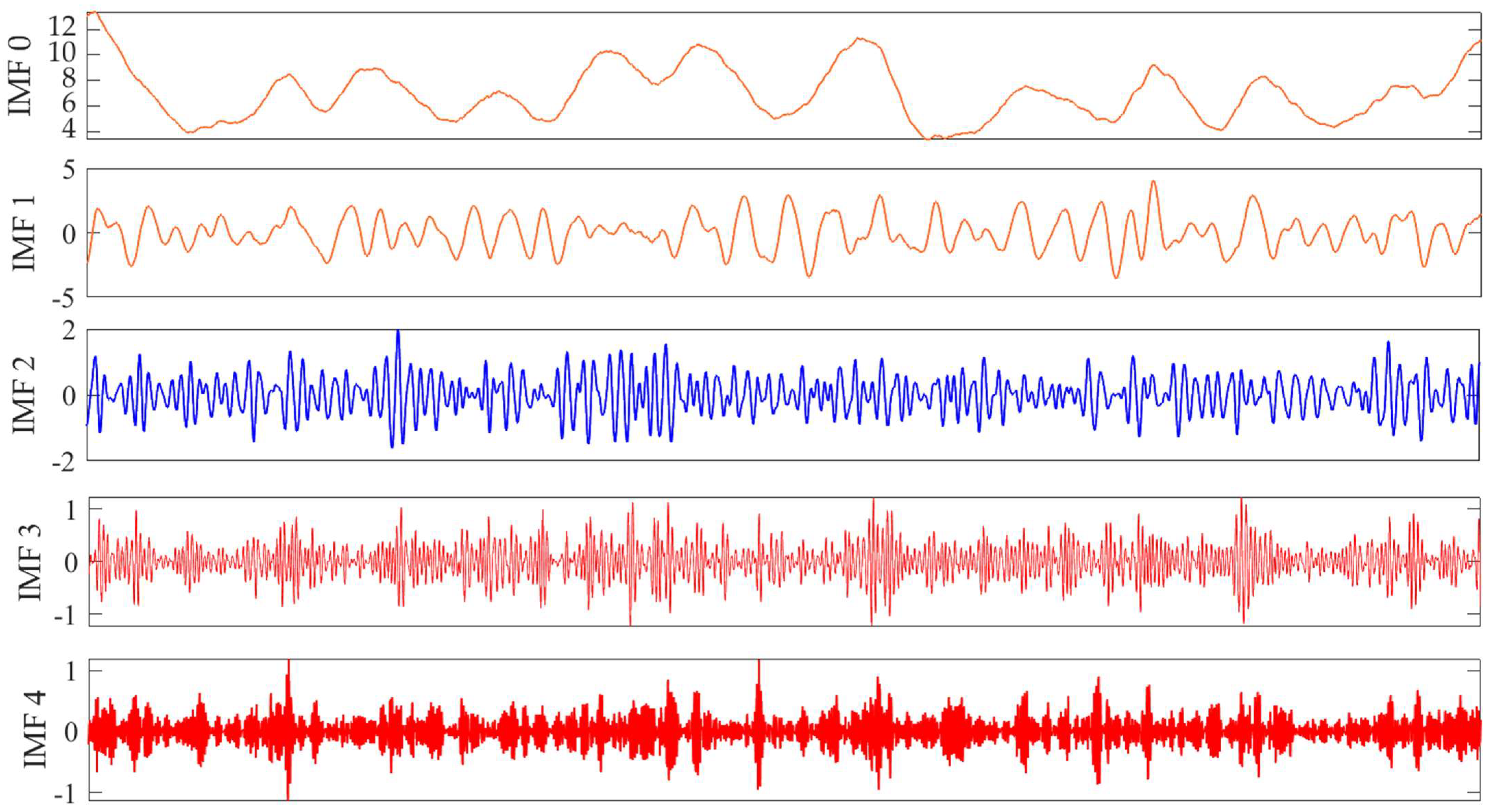
The decomposition time series method of VMD first needs to consider the number of decomposition layers. For different measurement methods, if the number of layers and time of K are different, this article sets K to 5. In other words, VMD decomposes the wind speed time series into five submodes, and Figure 3 shows the decomposition results. Submode 0 exhibits a significant long-term trend, with submodes from mode 1 to mode 4 being stationary or approximately stationary. However, whether the decomposition process can effectively improve wind speed prediction performance remains to be discussed.

In order to analyze the data characteristics, the complexity of modes was calculated, and different components were identified. The computational complexity uses the sample entropy. The larger the value, the more complex the time series is, but it cannot provide accurate values for small samples. Compared with the sample entropy, Lempel–Ziv is more robust and simple and can be identified using accurate forecasting models with low complexity in model construction. In the process of designing model matching, using the Lempel–Ziv method for component recognition has a high/low frequency and trend. The complexity patterns we calculated are shown in

Table 2. The Lempel–Ziv computational complexity index result.

Site	Quarter	VM0	VM1	VM2	VM3	VM4
Site 1	January	0.0380	0.1412	0.3341	0.4780	0.5867
	May	0.0353	0.1222	0.2879	0.4210	0.5079
	June	0.0353	0.1249	0.3151	0.4291	0.5422
	October	0.0353	0.1249	0.3205	0.4427	0.5459
Site 2	January	0.0435	0.1168	0.3422	0.4834	0.5867
	May	0.0380	0.1381	0.2906	0.4318	0.5405
	June	0.0598	0.2444	0.4536	0.5133	0.4753
	October	0.0380	0.1494	0.3531	0.4943	0.5595
Site 3	January	0.0489	0.1956	0.4047	0.5323	0.4889
	May	0.0435	0.1086	0.2770	0.4128	0.5350
	June	0.0407	0.1521	0.3096	0.4291	0.5215
	October	0.0380	0.1385	0.3232	0.4699	0.5378

. Taking January of Site 1 as an example, η 0.3657, VM0 to VM1 are low-trend components, VM2 is a trend component, and VM3 to VM4 are high-frequency components. Taking May of Site 2 as an example, η 0.325, VM0 to VM2 show a low-frequency trend, while VM4 shows a high-frequency trend.

Through the analysis of modal complexity and the identification of different components, the trend component and low-frequency component SVM model of 0–4 modes can be predicted; the corresponding high-component wind speed time series using the VMD-ESOA-SVM model and the respective predictions use different components, and the predicted results are generated by summarizing all the predictions.

4.3. Analysis Results

The section introduces the forecasting results of the seven models compared, including single mode (ELM, ENN, native, SVM), hybrid model (VMD-SVM, CEEMD-SVM), and ensemble model (VMD-ESOA-SVM).

4.3.1. Comparison of Single Model Forecasting Result

As a benchmark model, we considered the native, ELM, ENN, and SVM models. The native model is a special model of the moving average model. The ELM model is constructed by determining the number of hidden layer neutrons and the activation function of hidden layer neurons. The Elman neutral network has a multilayer structure similar to multilayer feedforward network. In addition, a single support vector machine was used in the proposed model, and the proposed model was verified.

Table 3. Evaluation results of Site 1 single model predicted wind speed data.

Quarter	Model	ELM	ENN	NAIVE	SVM
January	MAE (m/s)	0.4581	0.4745	0.5732	0.4358
	MAPE (%)	7.9795	8,3270	9.6524	7.3805
	MSE (m/s)	0.3847	0.4126	0.6120	0.3383
	RMSE (m/s)	0.6203	0.6424	0.7823	0.5816
May	MAE (m/s)	0.5214	0.7068	0.3542	0.5088
	MAPE (%)	11.1897	14.8360	12.5278	10.7653
	MSE (m/s)	0.5089	0.9853	0.2227	0.4951
	RMSE (m/s)	0.7134	0.9926	0.4719	0.7036
July	MAE (m/s)	0.5261	0.5918	0.7378	0.5830
	MAPE (%)	10.9802	11.2362	14.0424	10.5633
	MSE (m/s)	0.7041	0.6510	1.0532	0.7467
	RMSE (m/s)	0.8391	0.8061	1.0262	0.8641
October	MAE (m/s)	0.2597	0.2906	0.3542	0.2872
	MAPE (m/s)	9.1823	11.8149	12.5278	12.4397
	MSE (m/s)	0.1138	0.1379	0.2227	0.1380
	RMSE (m/s)	0.3373	0.3714	0.4719	0.3714

,

Table 4. Evaluation results of Site 2 single model predicted wind speed data.

Quarter	Model	ELM	ENN	NAIVE	SVM
January	MAE (m/s)	0.5559	0.8082	0.6412	0.4312
	MAPE (%)	8.4844	13.6201	9.6524	7.2888
	MSE (m/s)	0.5535	1.1685	0.7697	0.3342
	RMSE (m/s)	0.7440	1.0810	0.8773	0.5781
May	MAE (m/s)	0.5184	0.9452	0.7759	0.5163
	MAPE (%)	11.6065	25.3435	17.1347	11.4785
	MSE (m/s)	0.5090	1.4686	1.1671	0.5097
	RMSE (m/s)	0.7134	1.2119	1.0803	0.7140
July	MAE (m/s)	0.5929	0.6604	0.7701	0.5346
	MAPE (%)	12.8811	14.3133	15.6331	11.1130
	MSE (m/s)	0.6782	0.7924	1.1930	0.5435
	RMSE (m/s)	0.8235	0.8902	1.0922	0.7372
October	MAE (m/s)	0.2784	0.3252	0.3426	0.2825
	MAPE (m/s)	12.0581	15.7908	13.0775	12.7003
	MSE (m/s)	0.1298	0.1763	0.2058	0.1339
	RMSE (m/s)	0.3603	0.4199	0.4536	0.3660

and

Table 5. Evaluation results of Site 3 single model predicted wind speed data.

Quarter	Model	ELM	ENN	NAIVE	SVM
January	MAE (m/s)	0.5515	0.6098	0.6298	0.44271
	MAPE (%)	9.3581	10.4826	10.9273	8.2095
	MSE (m/s)	0.5618	0.6598	0.7298	0.3312
	RMSE (m/s)	0.7495	0.8123	0.8543	0.5755
May	MAE (m/s)	0.5102	0.7233	0.6971	0.5037
	MAPE (%)	11.6791	16.4352	15.9611	11.4336
	MSE (m/s)	0.4985	0.9726	0.9277	0.4780
	RMSE (m/s)	0.7060	0.9862	0.9632	0.6914
July	MAE (m/s)	0.4993	0.5182	0.6834	0.5146
	MAPE (%)	10.8072	10.8900	14.6324	10.6024
	MSE (m/s)	0.4901	0.5535	1.0139	0.5916
	RMSE (m/s)	0.7001	0.7440	1.0069	0.7292
October	MAE (m/s)	0.2503	0.2497	0.3364	0.2519
	MAPE (m/s)	9.5423	9.1076	12.4249	10.0926
	MSE (m/s)	0.1149	0.1155	0.2048	0.1163
	RMSE (m/s)	0.3390	0.3398	0.4526	0.3411

show the wind speed data calculation results of MAE, MAPE, MSE, and RMSE of a single model. In the comparison of these results, some useful information can be obtained. First, among these results, the native model is the worst. Second, due to the robustness and accuracy of the neural network model, the effect of the ENN model is average. Third, comparing the predicted performance indicators of the July wind speed data of Site 1, ELM performed to some extent better than SVM. However, SVM outperforms other models in wind speed data prediction at Sites 2 and 3, and the processing of wind speed data by variational mode decomposition technology improves the prediction performance of SVM. Therefore, the SVM model is generally superior to other models, and SVM is chosen as the benchmark model.

In Figure 4, it can be visually observed that in the histogram presented at Site 1, the height of the SVM is lower than the other models, indicating that the values of MAE, MAP E, MSE, and RMSE are low and thus the performance of its model is better, and the radar plot at Site 2 can directly show the relative advantages and disadvantages of different models, and the closer to the center of the radar plot, the better the performance of the model is, and at Site 3, the smaller the area occupied in the area plot indicates the better performance of the model, so the performance of the SVM in the single model comparison is the best. At the same time, we can also observe in that the values of MAE, MAPE, MSE, and RMSE in January and October are smaller than the values of the other two months, indicating that wind energy resources are abundant in January and October.

4.3.2. Comparison of Hybrid and Ensemble Models’ Forecasting Results

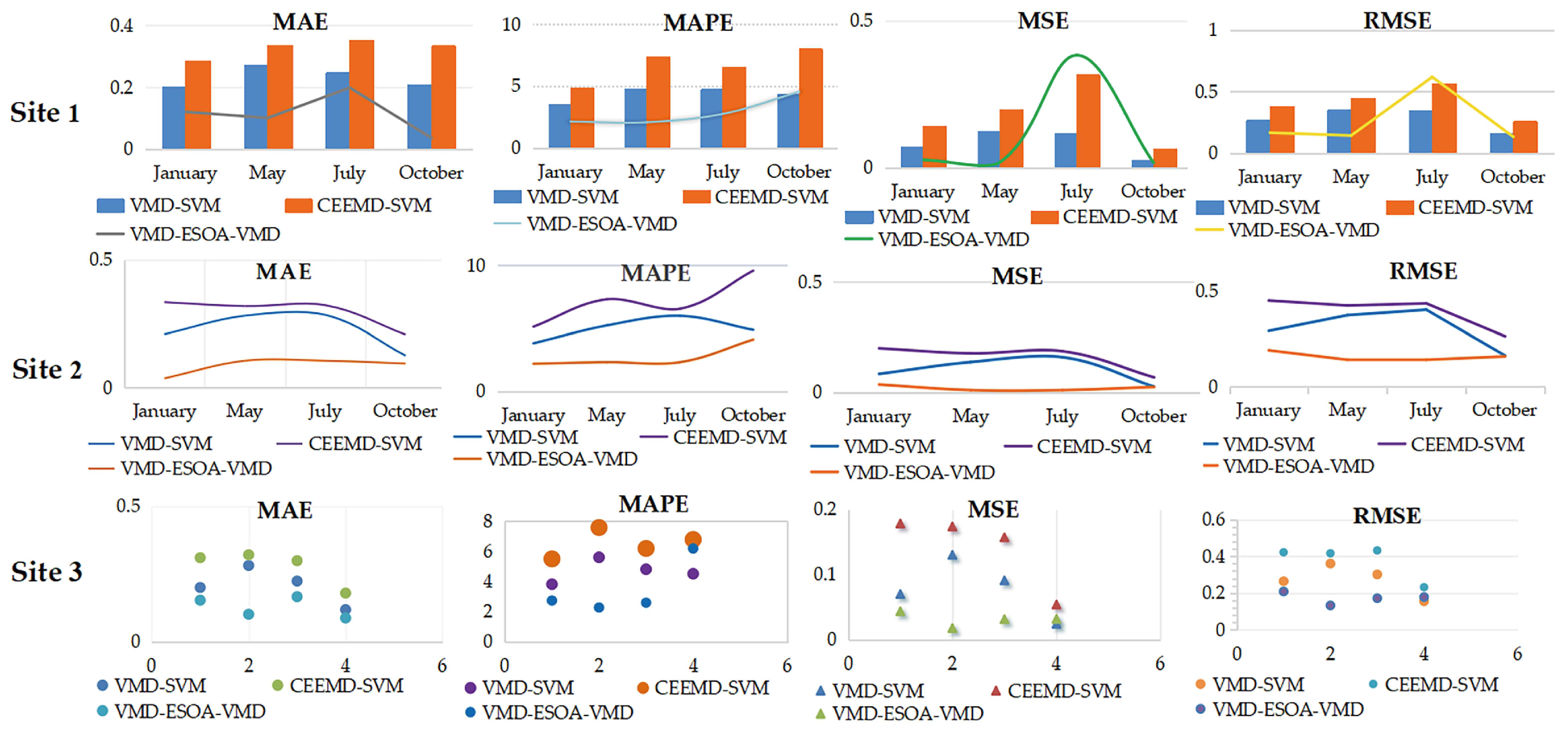
For the hybrid and ensemble models, firstly, the VMD method is more suitable for analyzing the wind speed time series decomposition process compared with the CEEMD method, as shown in

Table 6. Evaluation results of hybrid models for wind speed prediction at Site 1.

Quarter	Model	VMD-SVM	CEEMD-SVM	VMD-ESOA-VMD
January	MAE (m/s)	0.2017	0.2842	0.1204
	MAPE (%)	3.4757	4.8684	2.1164
	MSE (m/s)	0.0702	0.1409	0.0269
	RMSE (m/s)	0.2649	0.3754	0.1641
May	MAE (m/s)	0.2709	0.3362	0.1008
	MAPE (%)	4.7679	7.3896	2.0610
	MSE (m/s)	0.1233	0.1966	0.0200
	RMSE (m/s)	0.3511	0.4434	0.1413
July	MAE (m/s)	0.2476	0.3526	0.1989
	MAPE (%)	4.7489	6.5102	2.7455
	MSE (m/s)	0.1150	0.3149	0.3821
	RMSE (m/s)	0.3392	0.5612	0.6181
October	MAE (m/s)	0.1209	0.1994	0.0788
	MAPE (m/s)	4.3636	8.0397	4.5364
	MSE (m/s)	0.0243	0.0647	0.0171
	RMSE (m/s)	0.1559	0.2545	0.1308

,

Table 7. Evaluation results of hybrid models for wind speed prediction at Site 2.

Quarter	Model	VMD-SVM	CEEMD-SVM	VMD-ESOA-SVM
January	MAE (m/s)	0.2081	0.3330	0.0359
	MAPE (%)	3.8200	5.1387	2.1973
	MSE (m/s)	0.0839	0.1998	0.0356
	RMSE (m/s)	0.2897	0.4470	0.1886
May	MAE (m/s)	0.2802	0.3174	0.1049
	MAPE (%)	5.2315	7.3051	2.3198
	MSE (m/s)	0.1376	0.1772	0.0194
	RMSE (m/s)	0.3710	0.4210	0.1394
July	MAE (m/s)	0.2834	0.3211	0.2046
	MAPE (%)	5.9934	6.5565	3.8631
	MSE (m/s)	0.1595	0.1995	0.1149
	RMSE (m/s)	0.3993	0.4466	0.3390
October	MAE (m/s)	0.1245	0.2066	0.0941
	MAPE (m/s)	4.8853	9.5794	4.1096
	MSE (m/s)	0.0259	0.0683	0.0246
	RMSE (m/s)	0.1611	0.2613	0.1568

and

Table 8. Evaluation results of hybrid models for wind speed prediction at Site 3.

Quarter	Model	VMD-SVM	CEEMD-SVM	VMD-ESOA-SVM
January	MAE (m/s)	0.1992	0.3092	0.1523
	MAPE (%)	3.8186	5.5024	2.7347
	MSE (m/s)	0.0699	0.1780	0.0435
	RMSE (m/s)	0.2644	0.4219	0.2087
May	MAE (m/s)	0.2805	0.3199	0.1006
	MAPE (%)	5.6061	7.5843	2.2704
	MSE (m/s)	0.1299	0.1734	0.0177
	RMSE (m/s)	0.3605	0.4164	0.1330
July	MAE (m/s)	0.2230	0.2980	0.1654
	MAPE (%)	4.8147	6.1967	2.5930
	MSE (m/s)	0.0909	0.1867	0.0314
	RMSE (m/s)	0.3016	0.4321	0.1772
October	MAE (m/s)	0.1176	0.1786	0.0867
	MAPE (m/s)	4.5132	6.7879	6.1902
	MSE (m/s)	0.0242	0.0538	0.0318
	RMSE (m/s)	0.1557	0.2319	0.1784

. For four quarters of data from the three sites, the prediction evaluation results of the VMD-SVM model are better than those of the CEEMD-SVM model. For example, in the January evaluation results for Site 1, the MAE of CEEMD is 0.2842, MAPE is 4.8684, MSE is 0.1409, and RMSE is 0.3754, while the values of the MAE, MAPE, MSE, and RMSE of VMD-SVM are 0.2017, 3.4757, 0.0702, and 0.1649, respectively. This further indicates that VMD is superior to the CEEMD technique. It may also be due to the fact that the long-term prediction results of the CEEMD method are susceptible to unexploited factors, leading to its unpredictability. The decomposition process of the VMD method can effectively capture the internal patterns and better reconstruct multiple data for noise reduction decomposition. Secondly, it can be observed in Figure 5 that the proposed model outperforms the corresponding VMD-SVM-based multiscale hybrid model in terms of MAE, MAPE, MSE, and RMSE values for the VMD-ESOA-SVM model and the VMD-SVM model; the prediction performance of the former is better than the latter, indicating that the proposed multiscale model considers the prediction effect on different components.

5. Discussion

5.1. Data Decomposition Analysis

An important parameter in variational modal decomposition techniques is the number of decomposition layers, and the difference in the number of decomposition layers affects the performance of the predictive model, so a more accurate decomposition layer needs to be determined. As shown in

Table 9. Predictive performance of the proposed framework under different parameter optimization methods.

Site 1	MAE (m/s)	MAPE (m/s)	MSE (m/s)	RMSE (m/s)
k = 4	0.2413	4.8134	0.1393	0.3733
k = 5	0.2594	4.3320	0.1255	0.3543
k = 6	0.3680	6.2444	0.2511	0.5011
k = 7	0.3691	6.2285	0.2534	0.5034
k = 8	0.4049	7.0062	0.3141	0.5604

, when k takes different values, the results of the test model are also different, and the smaller the values of MAE, MAPE, MSE, and RMSE, the more accurate the number of decomposition layers. Although the value of k = 4 for MAE is slightly lower than the k = 5 value for MAE, it can be clearly observed in the table that when the number of decomposition layers’ k is set to 5, the values of MAPE, MSE, and RMSE are significantly lower than the other layers of k, so the number of decomposition layers is set to 5.

5.2. Analysis Parameter of Egret Population Optimization Algorithm

In the egret population optimization algorithm, lb is the lower bound of the definition domain and ub is the upper bound of the definition domain. We found that the difference in the upper and lower bounds of the definition domain affects the predictive performance of the proposed model, so we discussed the upper and lower values of the definition domain in order to choose a better definition domain. In Table 7, we can observe that when lb is set to 0.01 and ub is set to 2, the values of MAE, MAPE, MSE, and RMSE are significantly lower than other values of ub; further subdividing the value of lb, setting lb to 0.001 and 0.1 for comparison, through

Table 10. Different values of the definition domain of the egret population optimization algorithm.

Parameter	MAE (m/s)	MAPE (m/s)	MSE (m/s)	RMSE (m/s)
lb = 0.01 ub = 1	0.1539	2.8404	0.0456	0.2136
lb = 0.01 ub = 1.5	0. 1211	2.1468	0.0270	0.1644
lb = 0.01 ub = 2	0.1204	2.1170	0.0269	0.1642
lb = 0.01 ub = 2.5	0.1216	2.1322	0.0279	0.1670
Lb = 1 ub = 2	0.1204	2.1157	0.0269	0.1641
lb = 0. 1 ub = 2	0.1203	2.1157	0.0269	0.1641
lb = 0.001 ub = 2	0.1204	2.1164	0.0269	0.1641

we can observe that when the value of lb is 0.001, 0.01, 0.1, and 1, the values of MAE, MAPE, MSE, RMSE do not change significantly. The difference in the value of ub affects the performance of the model; therefore, we set the upper limit of the definition domain of the egret population optimization algorithm to 0.1 and the lower limit of the definition domain to 2.

5.3. DM Test

This study used the DM test to verify the effectiveness of the established model by comparing single models, mixed models, and VMD-ESOA-SVM integrated models. Based on the basic idea of the DM test, two hypotheses were proposed: the first hypothesis is that there is no significant difference in predictive performance between two models, while the second hypothesis is that there is a significant difference between two models.

Table 11. The values of DM tests of different models.

Site	Model	ELM	ENN	NAIVE	SVM	CEEMD-SVM	VMD-SVM
Site 1	January	14.3071 *	14.9625 *	14.8990 *	14.7210 *	2.9405 *	9.6457 *
	May	11.2756 *	12.9289 *	12.1116 *	12.1302 *	13.3440 *	10.1696 *
	June	2.0504 **	3.5568 *	5.7248 *	5.5924 *	2.4198 **	2.5458 *
	October	15.7204 *	16.2636 *	16.0923 *	19.4596 *	15.5613 *	4.4544 *
Site 2	January	14.8521 *	16.4252 *	14.1077 *	13.9161 *	12.1402 *	11.7077 *
	May	13.2756 *	12.4972	12.6159 *	12.7612 *	14.8045 *	13.3255 *
	June	12.1289 *	13.8208 *	13.6308 *	11.1556 *	3.2879 *	2.6548 *
	October	13.0896 *	160762 *	12.8064 *	14.7308 *	10.8990 *	1.4133 ***
Site 3	January	11.0441 *	14.1368 *	13.6279 *	11.8376 *	11.4672 *	9.2341 *
	May	13.7777 *	14.2897 *	13.5477 *	13.6060 *	15.7046 *	13.1152 *
	June	4.2221 *	7.3272 *	4.9505 *	9.87701 *	2.4563 **	2.3508 **
	October	9.9518 *	12.3137 *	10.1168 *	8.7520 *	2.1480 **	1.3556 ***

Note: * represents 1% significance level, ${\mathrm{z}}_{0.01/2}=2.58$; ** represents the 5% significance level, $z_{0.05/2}=1.96$; *** represents the 10% significance level, ${\mathrm{z}}_{0.10/2}=1.64$.

lists the DM test values of different models at three locations, and the results show that there is a significant difference of 1% between the proposed VMD-ESOA-SVM integrated model and other models, rejecting the original hypothesis, meanwhile leading to the conclusion that the proposed VMD-ESOA-SVM integrated model is significantly better than other models.

6. Conclusions

As an important part of green renewable energy, wind energy is widely used to cope with environmental pollution and climate change. Therefore, high-precision and high-efficiency wind speed forecasting methods are essential to improve the operational efficiency of wind power generation systems. In this study, we successfully developed a new ensemble model based on data denoising techniques, the egret optimization algorithm, and a support vector machine. We also used the VMD method to decompose wind speed time series into components with different features to improve prediction accuracy and reduce noise interference. We compared our results with the CEEMD ensemble model based on multiscale hybrid prediction and single models.

The relevant conclusions of the proposed ensemble model are as follows: Firstly, the number of decomposition layers in the data decomposition technique was discussed to determine the optimal parameter values by comparing the model performance such as MAE, MAPE, MSE, and RMSE to decompose, denoise, and reconstruct the original wind speed time series, which effectively improved the forecast accuracy of the model. Secondly, the definition domains of the parameters of the egret population optimization algorithm were discussed, and the optimal definition domain was determined by setting different definition domains for forecasting, the support vector machine was optimized, and the optimized support vector machine was further used to forecast the wind speed time series. The accuracy of the developed model was further demonstrated by comparing the developed model with other models and by DM testing. Based on the various analyses in this study, the developed ensemble model effectively improves the accuracy of wind speed prediction and provides a more effective and accurate method for wind speed forecasting.

In the future, it is recommended to consider and construct common multiscale hybrid models using other univariate forecasting methods. To determine the usefulness of multiscale models in time prediction, the accuracy of the proposed model parameters and the sensitivity of the procedure should be considered when using data for forecasting. By discovering more single and mixed models and conducting diversified comparisons, useful insights can be provided on how to improve the predictive performance of multiscale models and offer valuable recommendations.

References

- Zhao, W.G.; Wei, Y.M.; Su, Z.Y. One day ahead wind speed forecasting: A resampling-based approach. Appl. Energy 2016, 178, 886–901. [Google Scholar] [CrossRef]
- Yang, Y.; Zhou, H.; Gao, Y.C.; Wu, J.R.; Wang, Y.G.; Fu, L.Y. Robust penalized extreme learning machine regression with applications in wind speed forecasting. Neural Comput. Appl. 2022, 34, 391–407. [Google Scholar] [CrossRef]
- Jiang, Z.Y.; Che, J.X.; Wang, L.N. Ultra-short-term wind speed forecasting based on EMD-VAR model and spatial correlation. Energy Convers. Manag. 2021, 250, 114919. [Google Scholar] [CrossRef]
- Wang, X.W.; Li, P.B.; Yang, J.J. Short-term wind power forecasting based on two-stage attention mechanism. Inst. Eng. Technol. 2020, 14, 297–304. [Google Scholar]
- Santhosh, M.; Venkaiah, C.; Kumar, D.M.V. Ensemble empirical mode decomposition based adaptive wavelet neural network method for wind speed prediction. Energy Convers. Manag. 2018, 168, 482–493. [Google Scholar] [CrossRef]
- Tian, C.S.; Hao, Y.; Hu, J.M. A novel wind speed forecasting system based on hybrid data preprocessing and multi-objective optimization. Appl. Energy 2018, 231, 301–319. [Google Scholar] [CrossRef]
- Pan, K.K.; Qian, Z.; Chen, N.Y. Probabilistic short-term wind power forecasting using sparse Bayesian learning and NWP. Math. Probl. Eng. 2015, 2015, 785215. [Google Scholar] [CrossRef] [Green Version]
- Zhao, X.Y.; Liu, J.F.; Yu, D.R.; Chang, J.T. One-day-ahead probabilistic wind speed forecast based on optimized numerical weather prediction data. Energy Convers. Manag. 2018, 164, 560–569. [Google Scholar] [CrossRef]
- Song, J.J.; Wang, J.Z.; Liu, H.Y. A novel combined model based on advanced optimization algorithm for short-term wind speed forecasting. Appl. Energy 2018, 215, 643–658. [Google Scholar] [CrossRef]
- Xiao, L.Y.; Shao, W.; Jin, F.L.; Wu, Z.C. A self-adaptive kernel extreme learning machine for short-term wind speed forecasting. Appl. Soft Comput. 2021, 99, 106917. [Google Scholar] [CrossRef]
- Zhang, W.Y.; Zhang, L.F.; Wang, J.Z.; Niu, X.S. Hybrid system based on a multi- objective optimization and kernel approximation for multi-scale wind speed forecasting. Appl. Energy 2020, 277, 15561. [Google Scholar] [CrossRef]
- Singh, S.N.; Mohapatra, A. Repeated wavelet transform based ARIMA model for very short-term wind speed forecasting. Renew. Energy 2019, 136, 758–768. [Google Scholar]
- Shukur, O.B.; Lee, M.H. Daily wind speed forecasting through hybrid KF-ANN model based on ARIMA. Renew. Energy 2015, 76, 637–647. [Google Scholar] [CrossRef]
- Lydia, M.; Kumar, S.S.; Selvakumar, A.I.; Kumar, G.E.P. Linear and non-linear autoregressive models for short-term wind speed forecasting. Energy Convers. Manag. 2016, 112, 115–124. [Google Scholar] [CrossRef]
- Kavasseri, R.G.; Seetharaman, K. Day-ahead wind speed forecasting using ARIMA models. Renew. Energy 2009, 34, 1388–1393. [Google Scholar] [CrossRef]
- Liu, X.L.; Lin, Z.; Feng, Z.M. Short-term offshore wind speed forecast by seasonal ARIMA comparison against GRU and LSTM. Energy 2021, 227, 120492. [Google Scholar] [CrossRef]
- Cai, H.S.; Jia, X.D.; Feng, J.S.; Yang, Q.B.; Li, W.Z.; Li, F.; Lee, J. A unified Bayesian filtering framework for multi-horizon wind speed prediction with improved accuracy. Renew. Energy 2021, 178, 709–719. [Google Scholar] [CrossRef]
- Chen, Y.H.; He, Z.S.; Shang, Z.H.; Li, C.H.; Li, L.; Xu, M.L. A novel combined model based on echo state network for multi-step ahead wind speed forecasting: A case study of NREL. Energy Convers. Manag. 2019, 179, 13–29. [Google Scholar] [CrossRef]
- Wang, J.; Li, H.M.; Wang, Y.; Lu, H.Y. A hesitant fuzzy wind speed forecasting system with novel defuzzification method and multi-objective optimization algorithm. Expert Syst. Appl. 2021, 168, 114364. [Google Scholar] [CrossRef]
- Qu, Z.X.; Mao, W.Q.; Zhang, K.Q.; Zhang, W.Y.; Li, Z.P. Multi-step wind speed forecasting based on a hybrid decomposition technique and an improved back-propagation neural network. Renew. Energy 2019, 133, 919–929. [Google Scholar] [CrossRef]
- Guo, H.G.; Wang, J.Z.; Li, Z.W.; Jin, Y. A novel hybrid system based on multi-objective optimization for wind speed forecasting. Energy 2020, 146, 149–165. [Google Scholar]
- Jiang, P.; Yang, H.F.; Heng, J.N. A hybrid forecasting system based on fuzzy time series and multi-objective optimization for wind speed forecasting. Appl. Energy 2019, 235, 786–801. [Google Scholar] [CrossRef]
- Lopez, G.; Arboleya, P. Short-term wind speed forecasting over complex terrain using linear regression models and multivariable LSTM and NARX networks in the Andes Mountains, Ecuador. Renew. Energy 2022, 183, 351–368. [Google Scholar] [CrossRef]
- Chandra, D.R.; Kumari, M.S.; Sydulu, M.; Grimaccia, F.; Mussetta, M. Adaptive wavelet neural network based wind speed forecasting studies. J. Electr. Eng. Technol. 2014, 9, 1812–1821. [Google Scholar] [CrossRef] [Green Version]
- Liu, M.D.; Ding, L.; Bai, Y.L. Application of hybrid model based on empirical mode decomposition, novel recurrent neural networks and the ARIMA to wind speed prediction. Energy Convers. Manag. 2021, 233, 113917. [Google Scholar] [CrossRef]
- Jiang, P.; Liu, Z.K.; Niu, X.S.; Zhang, L.F. A combined forecasting system based on statistical method, artificial neural networks, and deep learning methods for short- term wind speed forecasting. Energy 2021, 217, 119361. [Google Scholar] [CrossRef]
- Jiang, P.; Wang, Y.; Wang, J.Z. Short-term wind speed forecasting using a hybrid model. Energy 2017, 119, 561–577. [Google Scholar] [CrossRef]
- Liu, D.; Niu, D.X.; Wang, H.; Fan, L.L. Short-term wind speed forecasting using wavelet transform and support vector machines optimized by genetic algorithm. Renew. Energy 2014, 62, 592–597. [Google Scholar] [CrossRef]
- Liu, H.; Mi, X.; Li, Y. Smart multi-step deep learning model for wind speed forecasting based on variational mode decomposition, singular spectrum analysis, LSTM network and ELM. Energy Convers. Manag. 2018, 159, 54–64. [Google Scholar] [CrossRef]
- Li, H.; Wang, J.; Lu, H.; Guo, Z. Research and application of a combined model based on variable weight for short term wind speed forecasting. Renew. Energy 2018, 116, 669–684. [Google Scholar] [CrossRef]
- Fu, W.L.; Fang, P.; Wang, K.; Li, Z.X.; Xiong, D.Z.; Zhang, K. Multi-step ahead short-term wind speed forecasting approach coupling variational mode decomposition, improved beetle antennae search algorithm-based synchronous optimization and Volterra series model. Renew. Energy 2021, 179, 1122–1139. [Google Scholar] [CrossRef]
- Chen, M.R.; Zeng, G.Q.; Liu, K.D.; Weng, J. A two-layer nonlinear combination method for short-term wind speed prediction based on ELM, ENN, and LSTM. IEEE Internet Things J. 2019, 6, 6997–7010. [Google Scholar] [CrossRef]
- Zhang, L.F.; Wang, J.Z.; Niu, X.S.; Liu, Z.K. Ensemble wind speed forecasting with multi-objective Archimedes optimization algorithm and sub-model selection. Appl. Energy 2021, 301, 117449. [Google Scholar] [CrossRef]
- Wang, J.Z.; Heng, J.N.; Xiao, L.Y.; Wang, C. Research and application of a combined model based on multi-objective optimization for multi-step ahead wind speed forecasting. Energy 2017, 125, 591–613. [Google Scholar] [CrossRef]
- Altan, A.; Karasu, S.; Zio, E. A new hybrid model for wind speed forecasting combining long short-term memory neural network, decomposition methods and grey wolf optimizer. Appl. Soft Comput. 2021, 100, 106996. [Google Scholar] [CrossRef]
- Wang, J.Z.; Du, P.; Niu, T.; Yang, W.D. A novel hybrid system based on a new proposed Algorithm-Multi-Objective Whale Optimization Algorithm for wind speed forecasting. Appl. Energy 2017, 208, 344–360. [Google Scholar] [CrossRef]
- Liu, Z.; Jiang, P.; Wang, J.Z.; Zhang, L.F. Ensemble forecasting system for short-term wind speed forecasting based on optimal sub-model selection and multi-objective version of mayfly optimization algorithm. Expert Syst. Appl. 2021, 177, 114974. [Google Scholar] [CrossRef]
- Liu, H.; Yang, R.; Duan, Z. Wind speed forecasting using a new multi-factor fusion and multi-resolution ensemble model with real-time decomposition and adaptive error correction. Energy Convers. Manag. 2020, 217, 112995. [Google Scholar] [CrossRef]
- Chen, Z.; Francis, A.; Li, S.; Liao, B.; Xiao, D.; Ha, T.T.; Li, J.; Ding, L.; Cao, X. Egret Swarm Optimization Algorithm: An Evolutionary Computation Approach for Model Free Optimization. Biomimetics 2022, 7, 144. [Google Scholar] [CrossRef]
Figure 1.
The proposed predictive modeling framework.
Figure 2.
Description of original wind speed data.
Figure 3.
VMD analysis of the daily ten-minute wind speed data decomposition process.
Figure 4.
Comparison of MAE, MAPE, MSE, and RMSE for single models at three sites.
Figure 5.
Comparison of MAE, MAPE, MSE, and RMSE for hybrid models at three sites.