
Dynamic Performance Analysis and Control Parameter Adjustment Algorithm for Flywheel Batteries Considering Vehicle Direct Action
School of Electrical and Information Engineering, Jiangsu University, Xuefu Road 301, Zhenjiang 212013, China
*
Author to whom correspondence should be addressed.
Energies 2023, 16(16), 5882; https://0-doi-org.brum.beds.ac.uk/10.3390/en16165882
Submission received: 2 July 2023
/
Revised: 27 July 2023
/
Accepted: 7 August 2023
/
Published: 9 August 2023
(This article belongs to the Special Issue Design and Control of Flywheel Energy Storage Systems)
Abstract
:Traditional methods often ignore the direct influences of vehicle vibration on the flywheel battery system, which leads to an inaccurate analysis of the dynamic performance of the flywheel battery system and its control effect. Therefore, to make up for the deficiencies of existing studies, a more accurate dynamic performance analysis method and efficient control parameter adjustment algorithm for flywheel batteries based on automotive direct action are proposed in this study. First, the influence of road conditions and vehicle driving conditions on the stability of a vehicle is analyzed primarily. Then, the vibration signal generated by the vehicle is transmitted to the vehicle’s magnetic flywheel battery system for analysis, and the accuracy of the analysis process is realized. Then, according to the stability analysis results for the direct action of the vehicle and the actual PID controller, the control parameter adjustment algorithm is summarized using the curve-fitting method. Finally, a performance test is carried out on the mobile experimental platform. Good experimental results show that the flywheel can quickly return to its equilibrium position and effectively reduce the influence of interference from road conditions and different working conditions and improve the robustness. Therefore, the correctness of the theoretical analysis and parameter adjustment method proposed in this paper was effectively verified.
1. Introduction
The flywheel battery system has advantages such as low environmental pollution, high energy conversion efficiency, and a long life cycle [1,2,3]. To achieve better energy conversion efficiency, a new numerical model method is developed for the thermal performance evaluation and wind resistance loss prediction of high-speed flywheel storage systems operating in atmospheric and partial vacuum conditions [4]. To improve the energy storage density, a mathematical model for the flywheel was established using the objective function and particle swarm optimization (PSO) algorithm, and a specific CFRP/Al hybrid co-curing flywheel was proposed [5]. The application of magnetic suspension flywheel battery technology to improve the energy efficiency of electric vehicles has attracted much attention in recent years. It is worth noting that an electric vehicle will produce vibration during the driving process due to its own driving condition and road conditions [6,7]. Therefore, the disturbances from driving and road conditions first act directly on the vehicle and are then transmitted to the flywheel battery system through the vehicle, where they affect the stability of the flywheel battery system [8,9,10]. However, the traditional method often regards the influence of these two aspects (the vehicle driving conditions and the road conditions) on the flywheel battery as direct effects and ignores the direct influence of the vibration of the vehicle itself on the flywheel battery system.
On the one hand, research on the flywheel battery system under the influence of vehicle driving conditions is as follows: To reveal how vehicle driving conditions influence the dynamic characteristics of a vehicular flywheel battery, a simplified experimental setup is proposed, and a series of computer-controlled sine and random vibration signals with different frequencies are applied [11]. To improve the control accuracy of a flywheel battery considering the influence of vehicle driving conditions, a dynamic correction model considering the influence of foundation motions is proposed, which has several submodules to cover as many driving conditions as possible [12]. To improve the stability of a vehicular flywheel battery, a novel stability control method based on the golden frequency section point is proposed for the gyroscopic effect and synchronous vibration caused by rotor mass imbalance [13]. However, it is worth noting that the existing perturbations to the flywheel battery system under vehicle driving conditions ignore the intermediate medium of the “vehicle itself”, i.e., existing studies approximate the perturbation signal of simulated vehicle driving conditions to be loaded directly to the flywheel battery system in the stability analysis process. In fact, the perturbation signal of vehicle driving conditions should be transmitted to the vehicle itself first, which affects the longitudinal and vertical stability of the vehicle and then affects the flywheel battery system mounted on the vehicle. Therefore, the existing research analyzes the disturbance signal of vehicle driving in an approximately equivalent way, which lacks analysis and control accuracy.
On the other hand, research on the flywheel battery system under the influence of road conditions is as follows: To prove the effectiveness of the proposed controller, the dynamic behavior of the flywheel under the action of road surface type and conditions is analyzed [14]. To explore the influence of irregular road conditions on the stability of a vehicle-mounted flywheel battery, different vibration tests on the active magnetic bearings supporting flywheel batteries have been performed [15]. To attenuate the disturbance response of the rotor system affected by vehicle motion, a technique for optimizing the acceleration feedforward compensator is proposed [16]. To deal with unmeasurable air gap velocity and generalized external disturbance effectively, a semi-supervised controller based on the DBN algorithm and output constraint controller is proposed [17]. To effectively suppress the time delay and uncertain dynamics of air gap vibration and thus significantly improve the performance of suspension control, an adaptive neural network controller with input delay compensation is proposed [18]. However, although there is much research on the influence of complex road conditions, most studies are limited to the analysis of its influence on the dynamic performance of magnetic suspension flywheel systems, and none of them use the “automobile” influenced by road conditions as the direct interference source of the flywheel battery system. Therefore, existing research methods are not accurate enough to analyze the influence of road conditions on vehicle flywheel battery systems. Furthermore, there is a lack of corresponding control criteria for summarizing and analyzing the affected laws.
Therefore, to make up for the deficiencies of existing studies, an accurate dynamic performance analysis method and high stability control strategy for flywheel batteries based on automotive direct action are necessary. Because the proportional–integral–derivative (PID) controller is a very practical controller, it has been widely used in many types of engineering applications, especially in the flywheel battery system. However, the dynamic model of the flywheel battery changes under different working conditions, so the control parameters of the PID controller need to be adjusted in real time. Therefore, this study uses a vehicle-mounted flywheel battery with a virtual inertia spindle based on a PID controller as an example to analyze and explore the control parameter adjustment algorithm. Firstly, a vehicle–road coupling model is established to study the influence of stability on the body by the vehicle itself driving and road conditions. Then, the vibration signal generated by the vehicle is transmitted to this vehicle-mounted magnetic suspension flywheel battery system, and then an accurate analysis is carried out. Then, based on the results from the stability analysis of the direct action of the vehicle, a control parameter adjustment algorithm is proposed. Finally, a performance test is carried out to verify the correctness of the theoretical analysis in this study.
2. Dynamic Performance Analysis of Flywheel Batteries Considering the Direct Vibration Effect of a Vehicle
2.1. Dynamic Performance Analysis Process and Setup
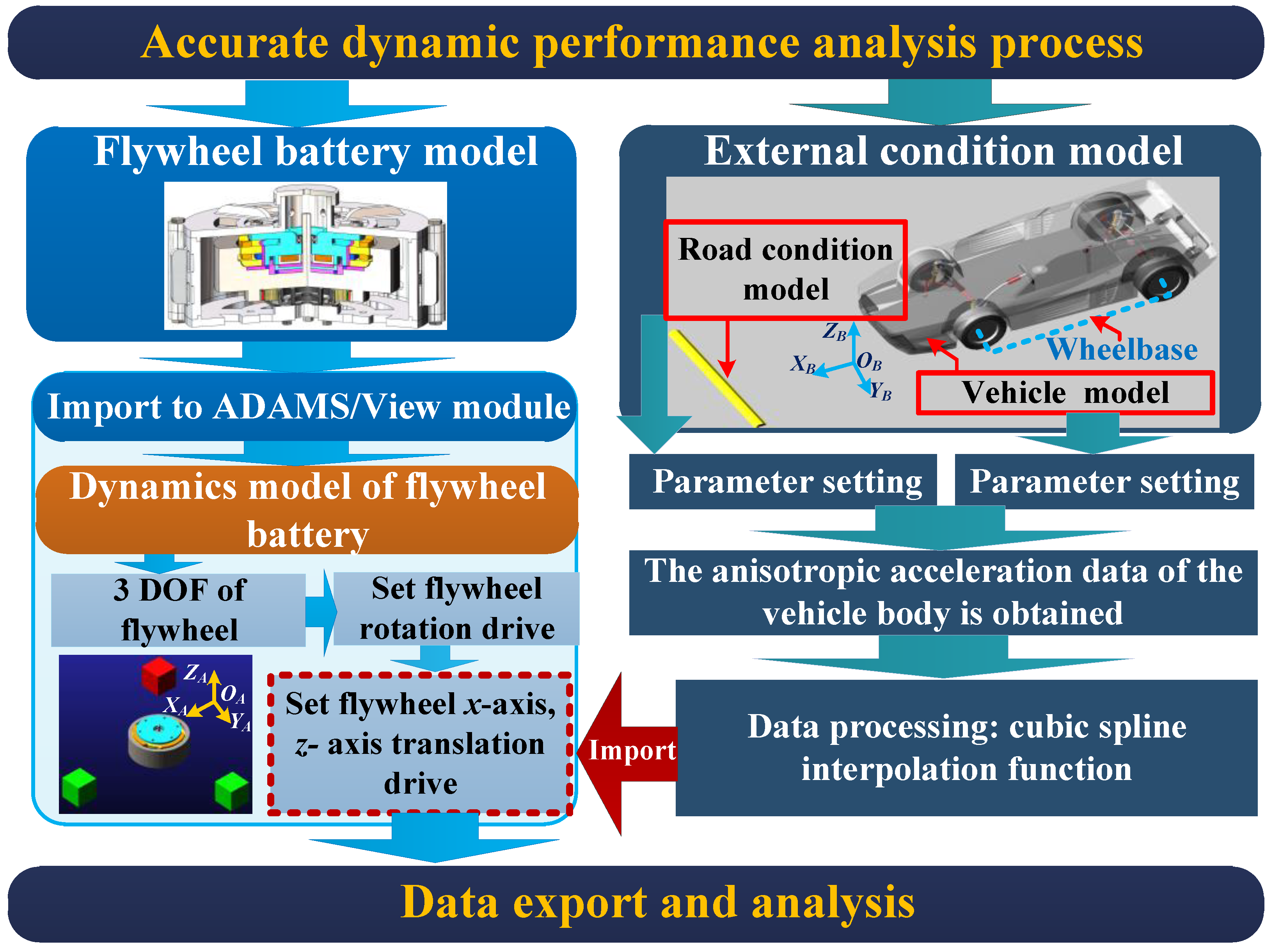
In this study, the influence of two key factors on the stability of a vehicle is primarily analyzed. In terms of road conditions, speed bump conditions are very common, especially in urban road conditions. This kind of operating condition interference can be regarded as extreme interference in the axial direction of a vehicle flywheel battery. In terms of vehicle driving conditions, the driving conditions of vehicles with different speeds can be regarded as the most typical interference in the radial direction of a vehicle flywheel battery, which is also worthy of attention and research. Therefore, the dynamic performance of the vehicular flywheel battery system under the influence of speed bumps and vehicle speeds is mainly analyzed in our study. The specific analysis process is shown in Figure 1. First, a vehicle model is created using the ADAMS/Car module, and then acceleration data for the external conditions under which the vehicle generates vibrations are obtained after setting the vehicle’s driving state and adding a road condition model. Finally, the vibration data are used as an external disturbance driver for the flywheel rotor using a cubic interpolation function in order to eliminate odd signals during vehicle travel and to accurately analyze the dynamic performance of the flywheel battery system.
As shown in Figure 1, the model of the vehicle-mounted flywheel battery with a virtual inertia spindle is first built using SolidWorks software. The key technical parameters are shown in Table 1. Additional details of the structure parameters, magnetic circuit, and working principle can be found in [19]. It is worth noting that this flywheel battery is a new concept battery that is more practical and conducive to large-scale popularization because of its high stability and superior energy storage characteristics. In addition, it can be mixed with other power systems used in vehicular systems to protect the original power battery or provide energy recovery during regenerative braking to improve energy efficiency. For example, it can be used as an energy buffer. The braking energy of the designed flywheel battery is 5.78 Wh, and the power density is 1214 W/kg. Furthermore, although the individual capacity of the flywheel battery is small, its capacity can be expanded using multiple cascades or by increasing the size and weight of the flywheel to adapt to various conditions. Of course, large-capacity flywheel batteries can be realized using cascading energy storage units. Furthermore, it can be realized using various inverters such as modular multilevel converters, cascaded H-bridge inverters, and so on.
Then, the equivalent flywheel rotor dynamics module is imported into the ADAMS/View module of ADAMS software, and each component of the model is constrained to assemble, an electromagnetic force is applied to the rotor, and the drive required in operation is simulated. Among them, the most critical step is to simulate the electromagnetic force. In the ADAMS/View module, three equivalent blocks are used to simulate the electromagnetic force constraints between the x, y, and z directions and the flywheel rotor, and the electromagnetic force formula in the corresponding direction is substituted when the force is set. In this way, the role of the magnetic bearings can be realized. At the same time, the drive flywheel unit is set to rotate around the z-axis, and the x- and y-axis translation drivers are also set. It is worth noting that in order to better illustrate the problem, two coordinate systems are defined in this paper: the coordinate system of the flywheel battery system is defined as OFXFYFZF, and the coordinate system of the vehicle is defined as OCXCYCZC. The external conditions model consists mainly of a vehicle model and a road conditions model. The vehicle model consists mainly of the front suspension system, rear suspension system, body, tire system, flywheel battery system, and other subsystems. Among them, the suspension, body, and tire systems are the template subsystems called using the ADAMS/Car module. As for the suspension requirements, this study takes into account the situation of ordinary vehicles and only needs to modify the spring stiffness in the subsystem to achieve the desired target virtual prototype. The vehicle parameters are shown in Table 2. (These parameters are taken from common vehicles currently on the market, where the front suspension deflection frequency is designed to be 1.44 and the rear suspension deflection frequency is 1.58).
For the completed external condition working model, the relevant parameters are set to obtain the relevant experimental vehicle acceleration data under simulated conditions. Then, the longitudinal and axial acceleration data on the body passing the speed bump are imported into the radial XF axis and axial ZF axis drivers of the corresponding flywheel dynamics model using a spline cubic interpolation function. The purpose of this method is to correct the singular signals in the vehicle driving data and simulate the running state of the vehicle system more truly. The driving state of the real vehicle is approximated to the maximum. Therefore, the dynamic performance of the flywheel rotor that can be directly acted on by the vehicle is realized.
2.2. Dynamic Performance Analysis of the Vehicle
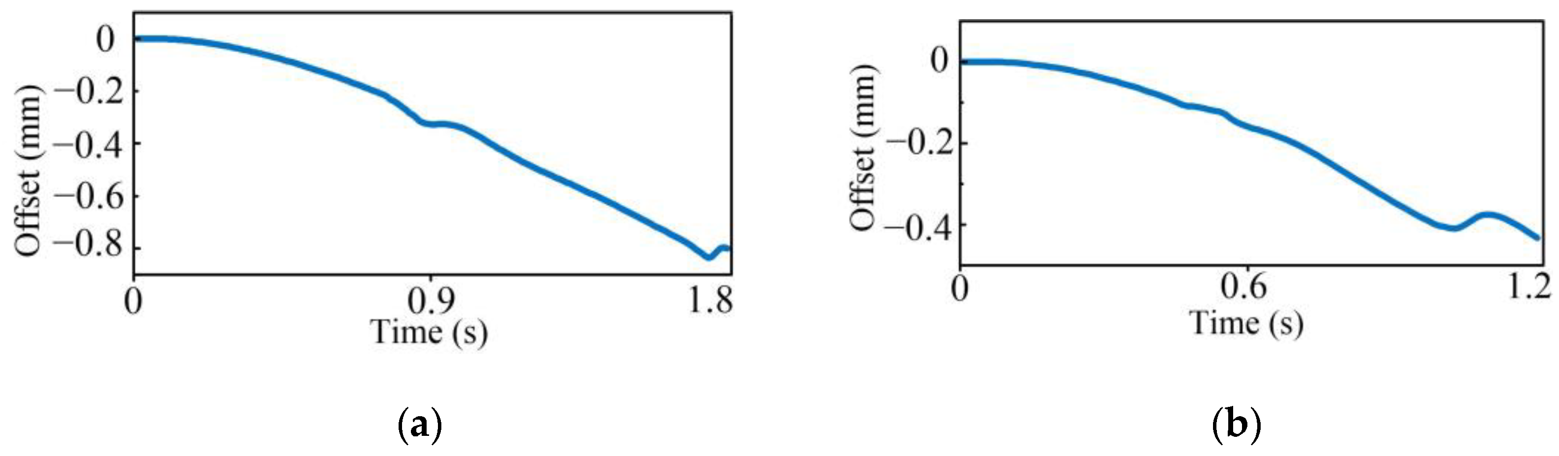
Based on the previous analysis, this section discusses the effect of driving conditions and road conditions on the vibration of the vehicle itself. The road condition model in the ADAMS/Car module refers to the speed bump on the actual road, and it is set up according to the most common speed bump height of 4 cm, length of 34 cm, and slope angle of 15 degrees. The driving state (speed) selection is made according to the normal road speed of vehicles in a city, i.e., 30 km/h to 60 km/h, but for speed bumps, the speed should be slowed down accordingly, generally to below 30 km/h. It is worth noting that, according to the above parameter settings, we find that the lateral displacement produced by the vehicle when driving at speeds slower than 30 km/h is within a small range, as shown in Figure 2. From Figure 2, it can be seen that the maximum lateral displacement of the body at both speeds is within 1 mm. This is because when a vehicle moves over a speed bump in a straight line (assuming that there is no unbalanced load and no lateral force collision or accident), the lateral force effect on the vehicle is much smaller than in the other two directions, so it is negligible. Therefore, this paper focuses on the dynamic response of a vehicle to a speed bump by observing the longitudinal and vertical acceleration of the body. Note that the lateral direction of the vehicle is defined as the YC direction, the longitudinal direction as the XC direction, and the vertical direction as the ZC direction.
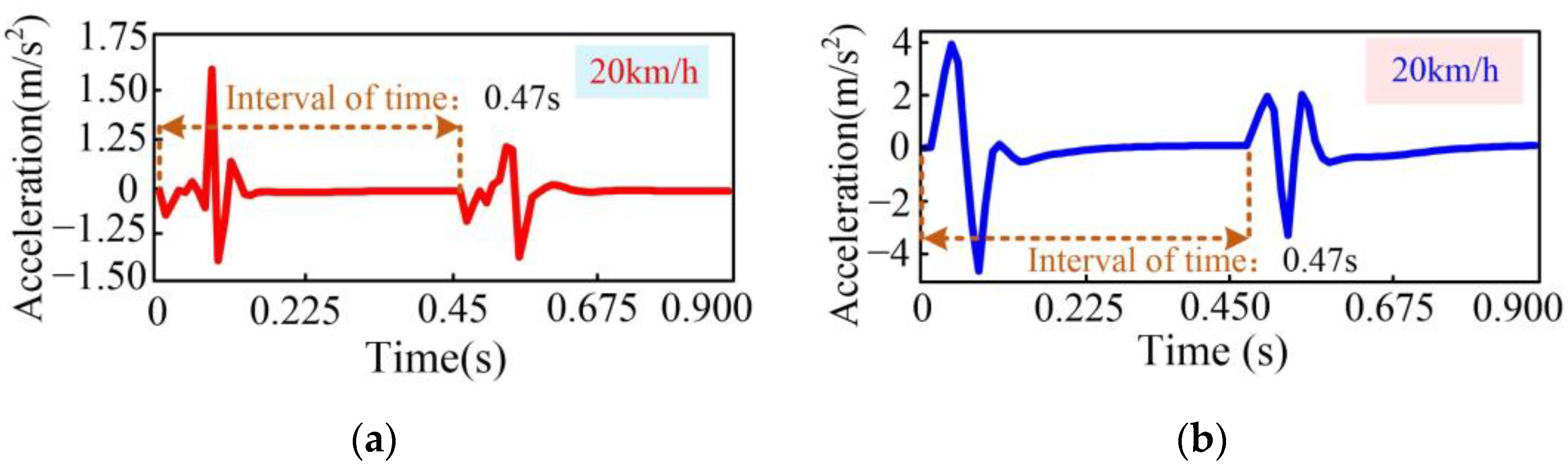
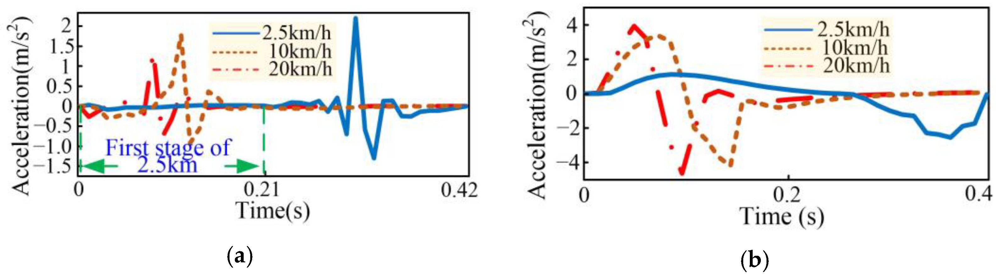
The body of the vehicle will be affected by the impact of the speed bump and vibration, resulting in instantaneous impact acceleration, when the vehicle passes over the speed bump at a certain speed. Figure 3 shows the impact acceleration along the XC and ZC directions after the body is disturbed when the vehicle passes over the speed bump at a speed of 20 km/h. As can be seen from Figure 3, two acceleration shocks are generated in two directions, respectively, and the time between two sequences of shocks is 0.47 s when the front wheel and the rear wheel pass over the speed bump, respectively. Further, Figure 4 continues to explore the change in acceleration when vehicles pass the same speed bump under the influence of different vehicle speeds. As can be seen from Figure 4a, the amplitude of impact acceleration caused by vibration in the body in the longitudinal direction (XC direction) is larger, and the time of occurrence is delayed when a vehicle passes over the same speed bump at a slower speed. However, on the contrary, the amplitude of the impact acceleration in the vertical direction (ZC direction) increases with an increase in vehicle speed.
Furthermore, from Figure 3 and Figure 4, it can be seen that when the vehicle passes over the speed bump at a certain speed, the curve of the impact acceleration produced will have a positive upward and a negative downward trend. That is because the vehicle goes through two stages of impact when passing over a speed bump.
Further, the details of the curve in Figure 4 are described as follows. The first stage is the impact between the wheel and the speed bump and thus the compression of the shock absorber, which is the process of the wheel rolling up the slope of the speed bump. From the law of conservation of momentum, it is known that the greater the speed, the greater the impact force. Therefore, the positive amplitude in Figure 4b increases with velocity. The second stage is the speed bump, which is the process of the wheel rolling down the ramp. However, as the speed increases, it is easy to jump, and the free fall motion is caused by the direct impact of the wheel on the ground. As can also be seen in Figure 4b, as the speed increases, the ground impact force (negative amplitude) suffered by the vehicle when it passes over the speed bump downhill also increases.
The acceleration of the body in the XC direction also varies according to these two phases. The difference is that in the first stage, the impact on the slope has little effect on the XC direction, so it can be seen from Figure 4a that the amplitude in this stage is small when the speed is low. Then, the shock absorber bounces back to form a vibration, producing a positive amplitude when it reaches the peak of the speed bump. As shown in Figure 4a, vibration effects are different at different speeds. The amplitude decreases with increasing velocity, which is related to the body’s frequency response. The higher the speed, the harder it is to create resonance when the shock absorber bounces before the body has a chance to bounce. The same is true for negative amplitudes.
2.3. Dynamic Performance of the Flywheel Battery Based on the Vehicle Direct Action
Based on the above analysis results, the dynamic performance of the flywheel battery under the direct action of the vehicle is analyzed. Combined with the definition of the two coordinate systems shown in Figure 1 (the flywheel rotation axis of the flywheel battery is perpendicular to the vehicle chassis horizontal plane) and the analysis process shown in the figure, the corresponding dynamic performance of different speeds over the speed bump is obtained. Meanwhile, the running speed of the flywheel is set to 1800 r/min. It is worth noting that in order to highlight the influence of the speed bump road conditions on the stability of the flywheel battery system, the influence of the gyroscopic effect generated by the high-speed flywheel is excluded.
Since the PID controller is very practical and has been tested in the magnetic suspension control system, the classical and practical PID controller is given priority in the magnetic control system. The classical PID control strategy is used to adjust the stable suspension of the rotor, and its transfer function is as follows:
where kp, ki, and kd are proportionality, integral, and differential coefficients, respectively, and Td is the differential time constant.
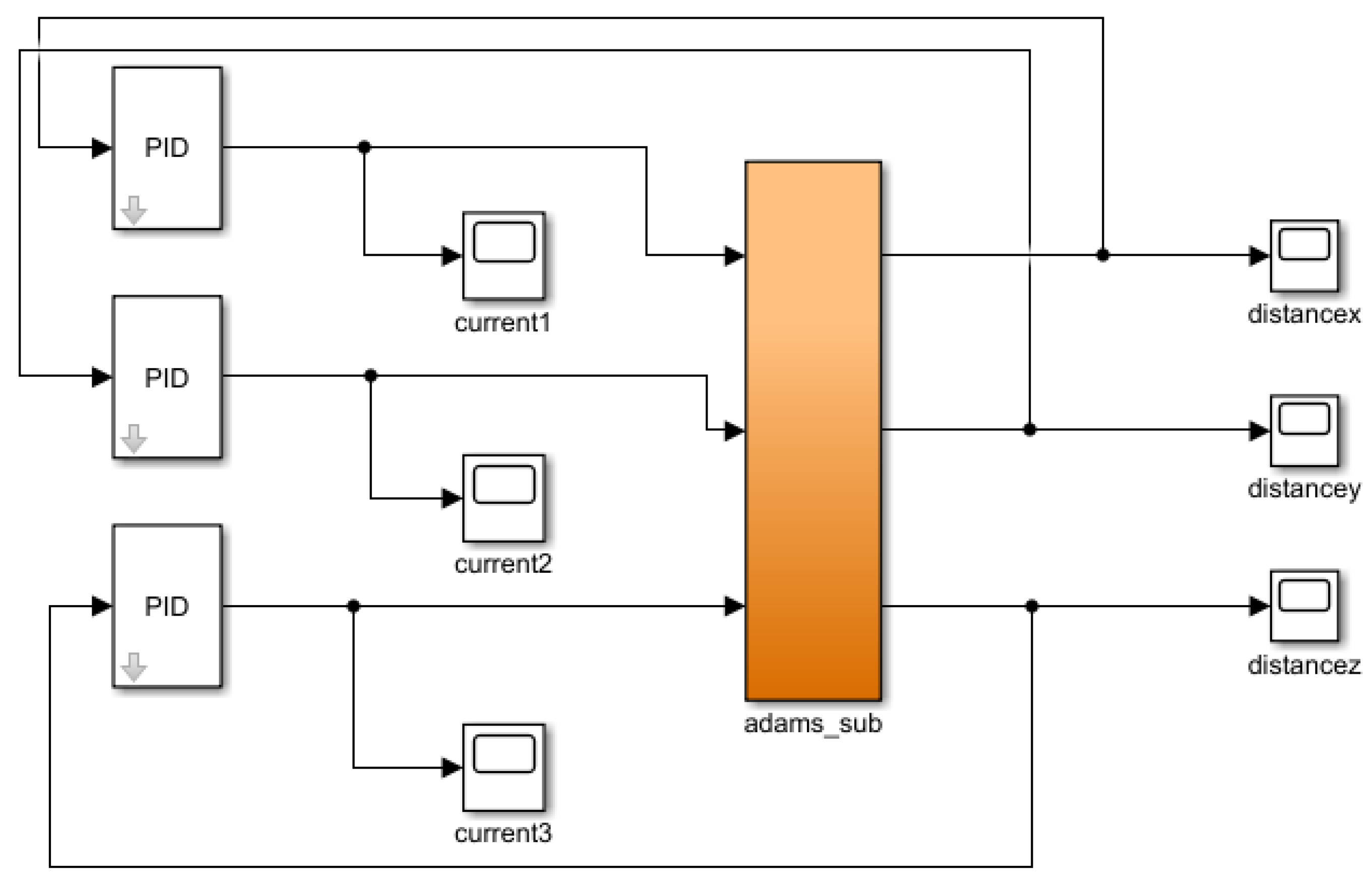
Figure 5 shows the control block diagram using the classical PID controller and ADAMS co-simulation. The dynamic behavior of the suspension rotor based on the suspension control system can be obtained using the control block diagram shown in Figure 5.
Note that the criterion for defining the control parameters of the optimal PID controller is whether the overshoot of the control result is the minimum, and the adjustment time is the shortest under the control of the parameter.
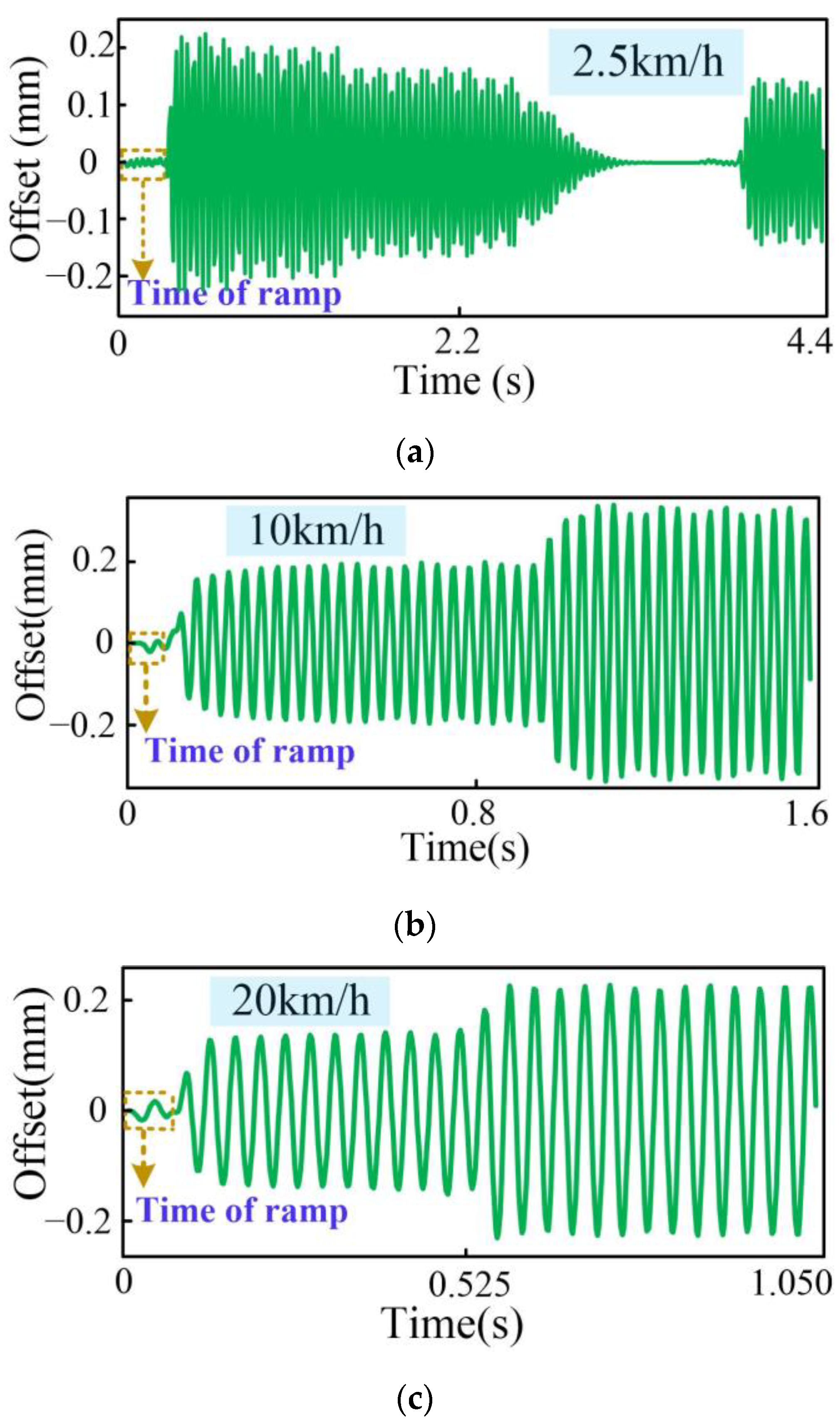
Figure 6 shows the dynamic performance of the flywheel in the XF direction when the magnetic suspension control system is applied when the vehicle passes over the 4 cm speed bump at different speeds. However, Figure 7 shows the dynamic performance of the flywheel without a magnetic suspension control system in the XF direction under the same motion conditions. As can be seen from Figure 6, the flywheel vibrates very strongly because it is not controlled by the magnetic suspension control system. In addition, it can be found that the flywheel offset is small at the beginning and that the flywheel offset tends to decline in the radial XF direction when the vehicle crosses the same speed bump at a higher speed. These are consistent with the acceleration effects caused by the two phases analyzed in Figure 4.
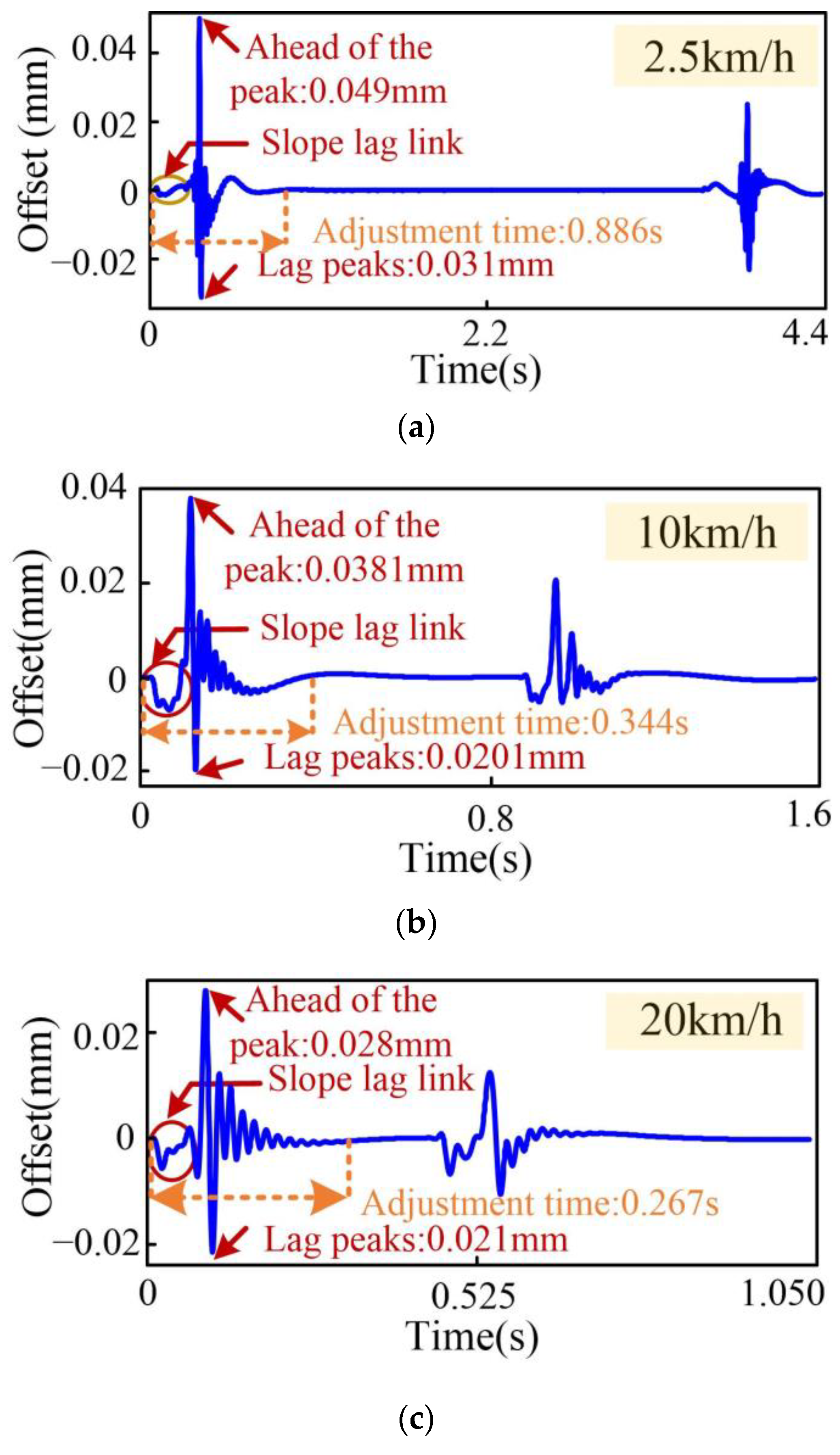
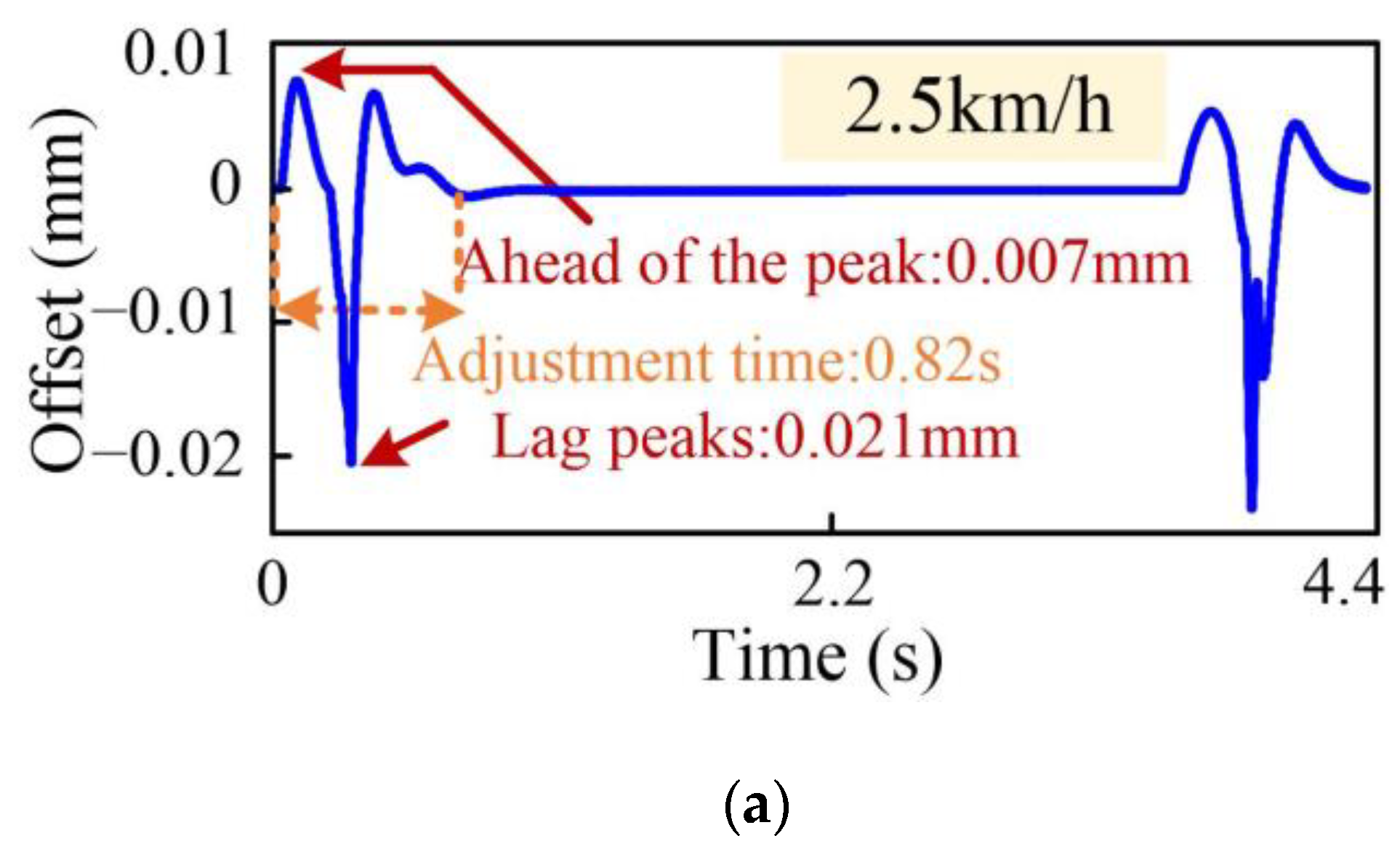
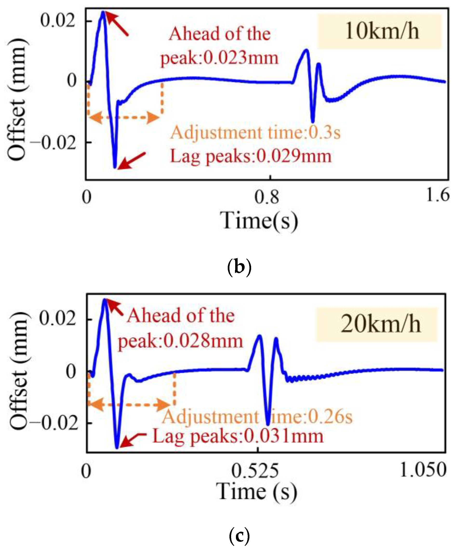
From Figure 7, it can be seen that the vibration in the flywheel is significantly improved under the action of the magnetic control system. As shown in Figure 7a, it can be seen that when the front and rear wheels pass over the speed bump at the speed of 2.5 km/h, the flywheel will return to the stably suspended state in a short time. In addition, it can be seen from Figure 7b,c that when the vehicle runs to the speed bump at a faster speed, the flywheel becomes more tortuous in the process of achieving smooth suspension due to the violent impact but stable suspension can be achieved in the end. Note that the classic PID controller is used in the control system. And in Figure 7, each group of experiments achieved stable suspension under optimal PID control parameters.
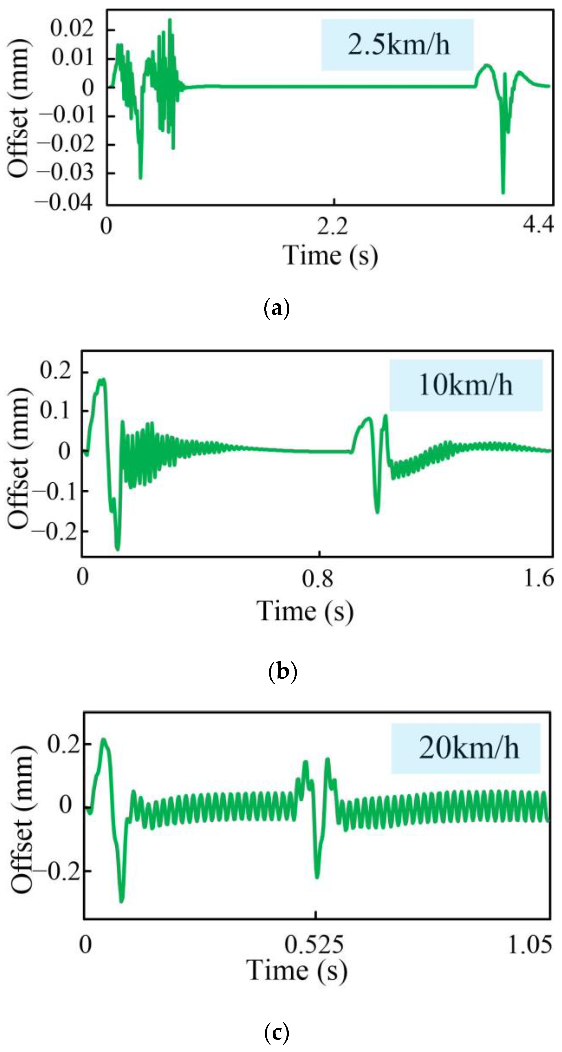
Figure 8 shows the dynamic performance of the flywheel in the ZF direction when the magnetic suspension control system is applied when the vehicle passes over the 4 cm speed bump at different speeds. In contrast, Figure 9 shows the dynamic performance of the flywheel without a magnetic suspension control system in the ZF direction under the same motion conditions. The front and rear wheels of the vehicle will have two instantaneous impacts when they pass over the speed bump, as shown in Figure 8. As the speed of the vehicle increases, the impact force also increases. Therefore, the displacement amplitude in the ZF direction increases significantly when the flywheel is not controlled, which also leads to a longer and more amplified vibration process in that direction. As shown in Figure 9, similar to the radial control result, when the vehicle runs to the speed bump at a faster speed, the flywheel becomes more tortuous in the process of achieving smooth suspension due to the violent impact, but a stable suspension can be achieved in the end.
3. Parameter Adjustment Algorithm Based on Accurate Dynamic Performance Analysis
As the classical PID controller can be used to achieve a relatively stable suspension of the flywheel, as shown in Figure 7 and Figure 9, methods to further improve the efficiency of parameter adjustment and control accuracy according to the summarized dynamic performance of the flywheel are worth studying. Because the proportional control parameters and derivative control parameters are the most difficult to adjust, the focus of the next sections is on the regulation of these two parameters.
3.1. Dynamic Performance of the Flywheel Battery Based on Vehicle Direct Action
Taking the PID control parameters adjusting the flywheel in Figure 7 as an example, the connection between the parameter setting and the dynamic performance of the flywheel is illustrated. As shown in Figure 7, the first stage’s impact force at 2.5 km/h has a long time span of 0.21 s and a small intensity, and the flywheel is affected by it with a relatively small amplitude. Therefore, the corresponding scaling parameters are small and can be controlled at the optimum amplitude. For 10 km/h and 20 km/h, the scale parameter should increase with speed as the impact force increases, while the time spectrum also increases with the speed (more high-frequency components) in order to speed up the response process and suppress high frequencies. For the later vibration process, at 2.5 km/h, although the amplitude is maximum, the process is decaying, while at the remaining two speeds, the form increases. Also, the differential parameter has an increasing trend with increasing stability due to the presence of an increasing high-frequency component. This is because the differential parameter acts as a suppression of bias in any direction in the response process. These parameter adjustments also apply to the rear wheel, as its amplitude changes are the same as those in the front wheel.
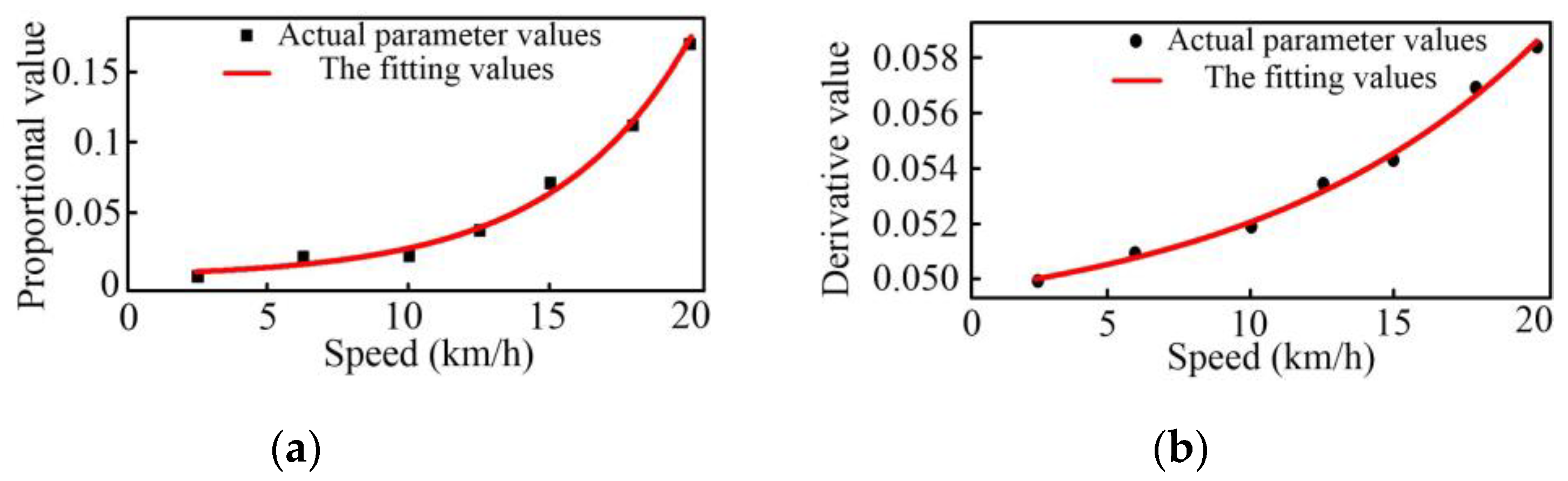
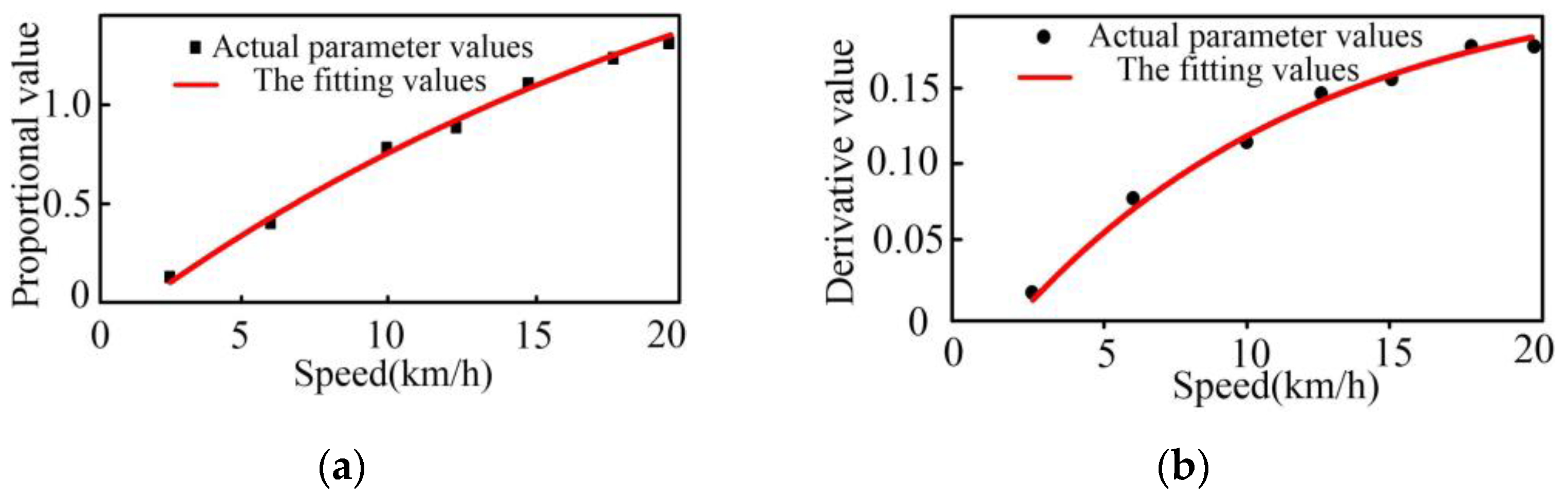
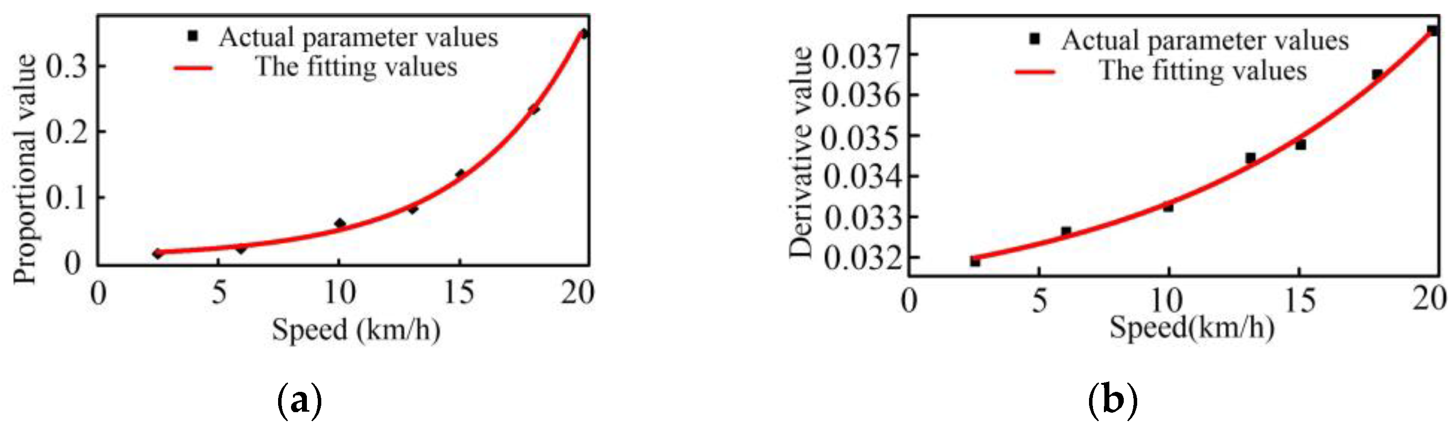
Further, according to the analysis results above, the adjustment rule for the radial control parameters is analyzed using seven sampling speeds passing over a 4 cm speed bump as an example. The fitting results for the proportional coefficients versus speed (Figure 10a) and the fitting results for the derivative coefficients versus speed (Figure 10b) can be obtained according to the seven sets of data. The relationships between the main parameters of radial control are obtained as follows:
where kp1 and kd1 are the proportional and derivative parameters for the radial PID controller when the vehicle passes over the 4 cm speed bump, respectively, and vx is the vehicle speed.
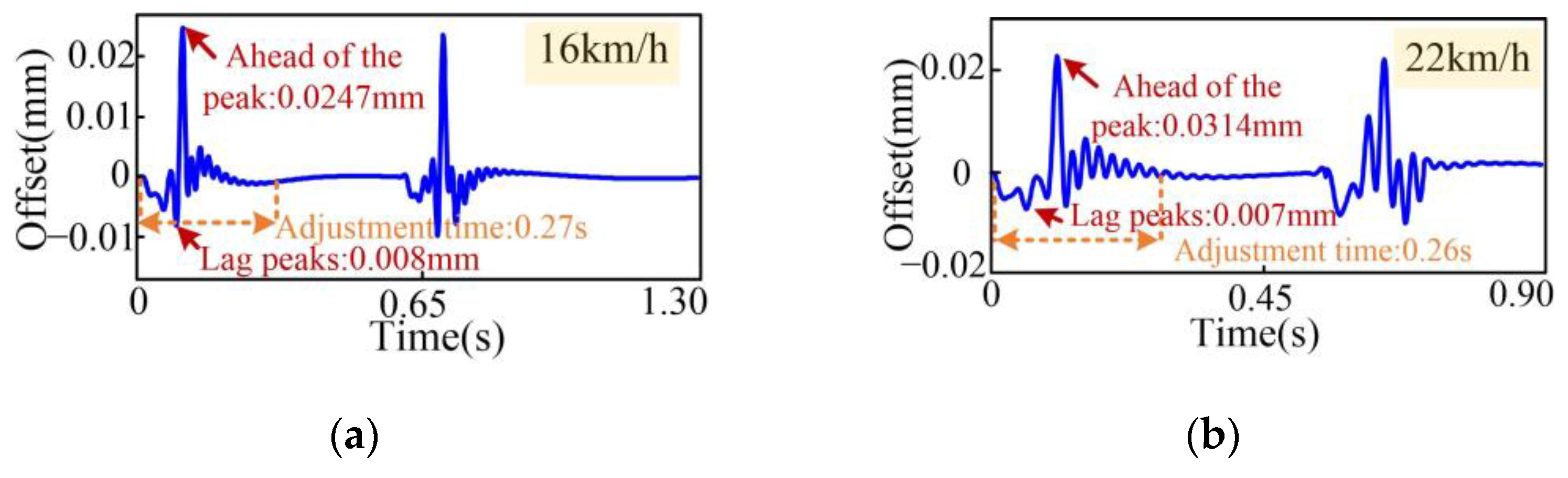
Further, to verify the correctness of the fitted curve equations for the radial control parameters, two speeds of 16 km/h and 22 km/h are randomly selected (not one of the seven data sampling points) in the speed range of 30 km/h to verify whether the corresponding parameters are valid. Using Equations (2) and (3), the corresponding proportional and derivative values can be calculated. According to the calculation, when the vehicle speed is 16 km/h, the proportional parameter is 0.078 and the derivative parameter is 0.055, while when the speed is 22 km/h, the proportional parameter is 0.264 and the derivative parameter is 0.061. Based on the control parameters, the dynamic performance diagram of the flywheel is obtained. From Figure 11, it can be seen that under the control of the control parameters calculated using Equations (2) and (3), the flywheel is disturbed to a certain degree when the front and rear wheels cross over the speed bump for two times successively, but it can recover to the stable suspension at the equilibrium position after a very short time adjustment.
3.2. The Axial Control Parameter Adjustment Law Based on Accurate Dynamic Performance Analysis
Similarly, taking the PID control parameters adjusting the flywheel in Figure 9 as an example, the connection between parameter setting and the dynamic performance of the flywheel is illustrated. As shown in Figure 8, with an increase in vehicle speed, the impact response of the flywheel is greater. Therefore, proportional parameters and differential parameters in this direction should be increased. As can be seen from the control effect shown in Figure 9, the amplitude can be reduced to a large extent, and the vibration can be suppressed using this parameter adjustment approach.
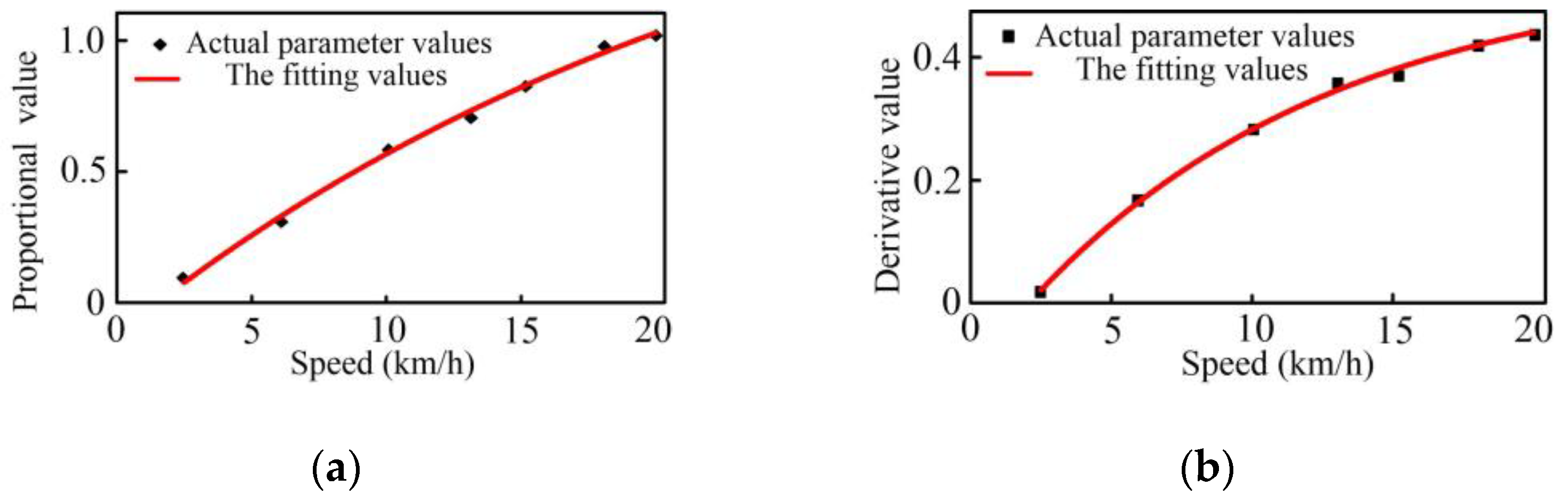
Further, according to the analysis results above, the adjustment rule for the axial control parameters is analyzed using seven sampling speeds passing over a 4 cm speed bump as an example. The fitting curves are shown in Figure 12. According to the fitting results for axial control, the following relationships can be obtained:
where kp2 and kd2 are the proportional and derivative parameters, respectively, for the axial PID controller when the vehicle passes over the 4 cm speed bump.
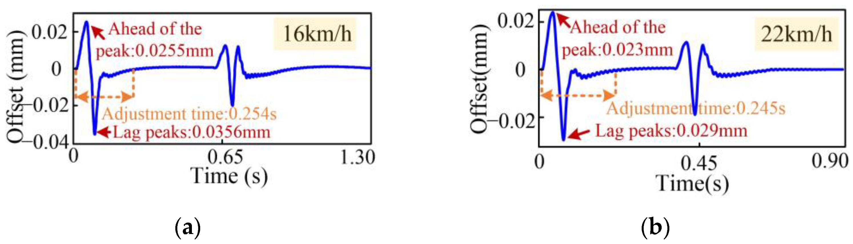
According to Equations (4) and (5), the corresponding proportional and derivative values can be calculated. Based on the control parameters, the dynamic performance diagram of the flywheel is obtained. According to the calculation, when the vehicle speed is 16 km/h, the proportional parameter is 1.14 and the derivative parameter is 0.164, while when the speed is 22 km/h, the proportional parameter is 1.45 and the derivative parameter is 0.191. As can be seen from Figure 13a, the flywheel battery system effectively reduces the disturbance caused by the front wheel excitation, with a maximum forward movement of 0.0255 mm and a maximum lag of 0.0356 mm, which can quickly realize the position balance, and the adjustment time is 0.254 s. Similarly, the disturbance caused by the rear wheel when it crosses over the speed bump is also effectively controlled. Furthermore, as shown in Figure 13b, the maximum advance offset and hysteresis offset of the disturbance are suppressed at 0.023 mm and 0.029 mm, respectively. In addition, there is also a significant control effect on the subsequent continuous disturbance with an adjustment time to the equilibrium position of 0.245 s. Therefore, according to the effective controller parameters obtained, although the flywheel is disturbed to a certain extent when the front and rear wheels pass over the speed bump twice in a row, the flywheel will quickly return to the equilibrium position after a very short time adjustment.
3.3. General Parameter Adjustment Algorithm Based on Accurate Dynamic Performance Analysis
If the height of a speed bump is greater or less than 4 cm, the precise analysis method shown in Figure 1 is also applicable. Therefore, a speed bump with a height of 7 cm is taken as an example for another calculation.
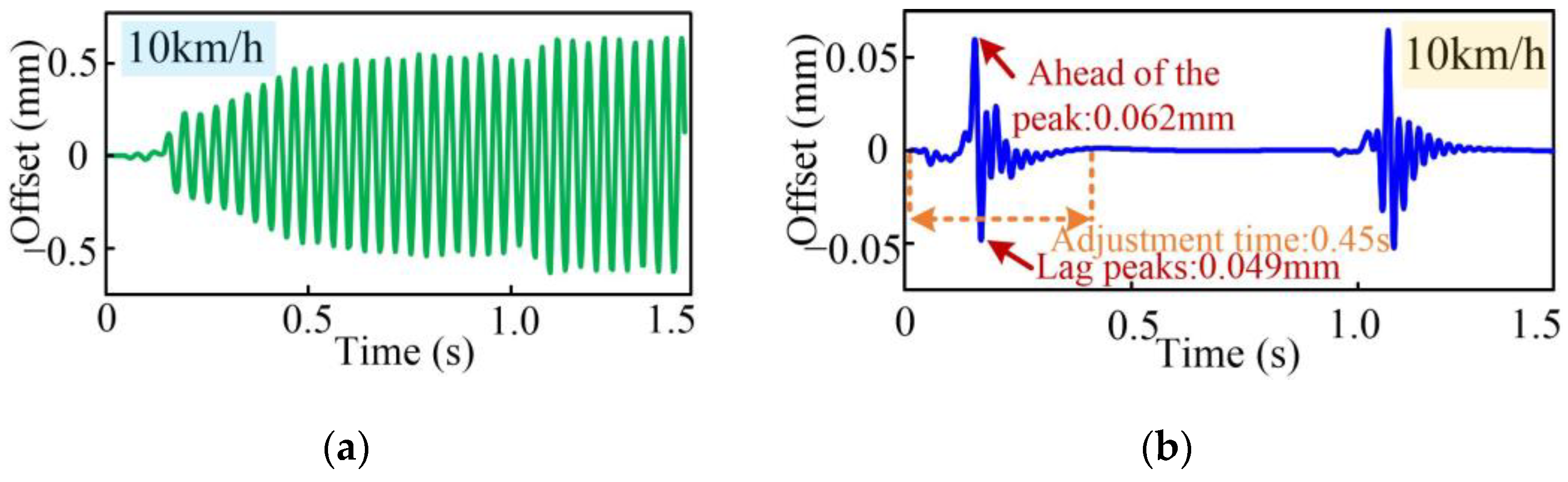
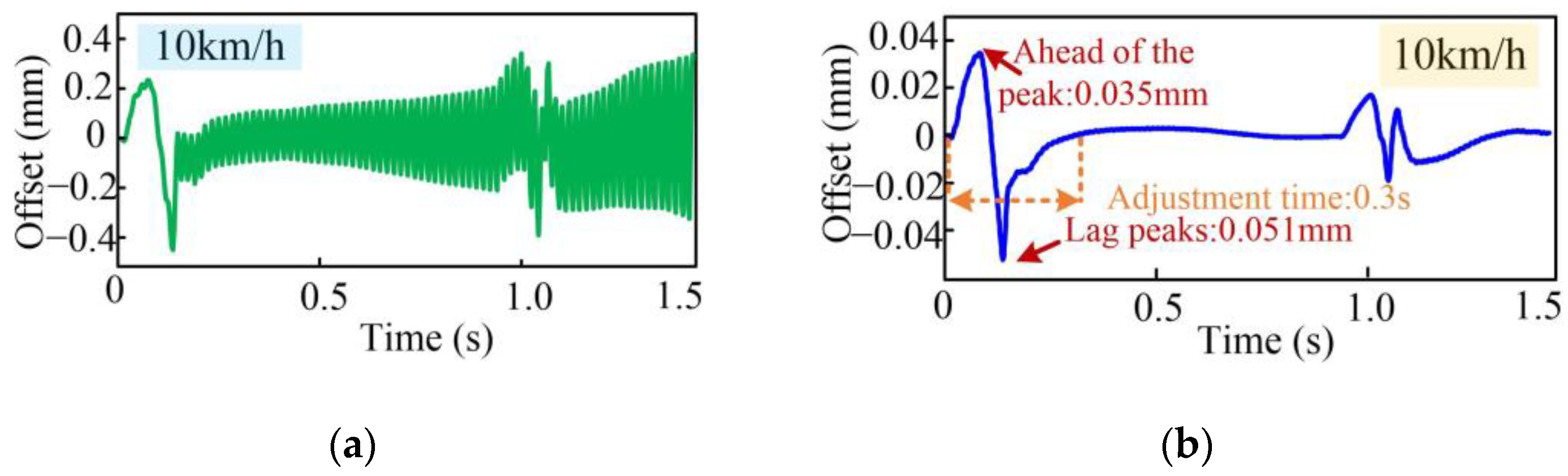
Figure 14 and Figure 15 show the dynamic performance diagrams of the flywheel in uncontrolled and controlled mode when the vehicle speed is 10 km/h passing over the 7 cm speed bump. As can be seen from the figures, the dynamic response results for the flywheel in the radial and axial directions are the same when the vehicle passes over the 7 cm speed bump and when the vehicle passes the 4 cm speed bump. The difference between them is only in magnitude.
Therefore, the remaining speeds are also analyzed for the 7 cm speed bump to observe the optimum parameters under their respective control and to summarize the laws. Figure 16 shows the fitting for radial control parameters when the vehicle passes over the 7 cm speed bump, and the formulas are as follows:
where kp3 and kd3 are the proportional and derivative parameters, respectively, for the axial PID controller when the vehicle passes over the 7 cm speed bump.
Figure 17 shows the results for the fitting of the parameters in the ZF direction, respectively. As a result, the following relationship can be obtained:
where kp4 and kd4 are the proportional and derivative parameters, respectively, for the axial PID controller when the vehicle passes over the 7 cm speed bump.
According to the above analysis, considering the most typical speed bump and vehicle speed, the general parameter adjustment algorithm for the PID controller of a flywheel battery under the influence of the two key factors, i.e., the road conditions and vehicle driving factors, can be obtained:
where Rp and Rd are the proportional and derivative parameters, respectively, for the radial PID controller and h is the height of the speed bump.
where Ap and Ad are the proportional and derivative parameters, respectively, for the axial PID controller.
Note that in urban road conditions, the commonly used speed bump is greater than or equal to 4 cm, so the 4 cm speed bump is used as a benchmark to deduce its general formula. Therefore, Equations (12) and (13) are general formulas for speed bumps with heights greater than or equal to 4 cm. If there are special circumstances, such as the occurrence of a speed reducer height less than 4 cm, it is completely possible to list the general formulas for PID controller parameter adjustment for a speed bump height less than 4 cm according to the derivation formula and curve fitting methods.
4. Experimental Results and Analysis
4.1. Experiment Platform and Control System
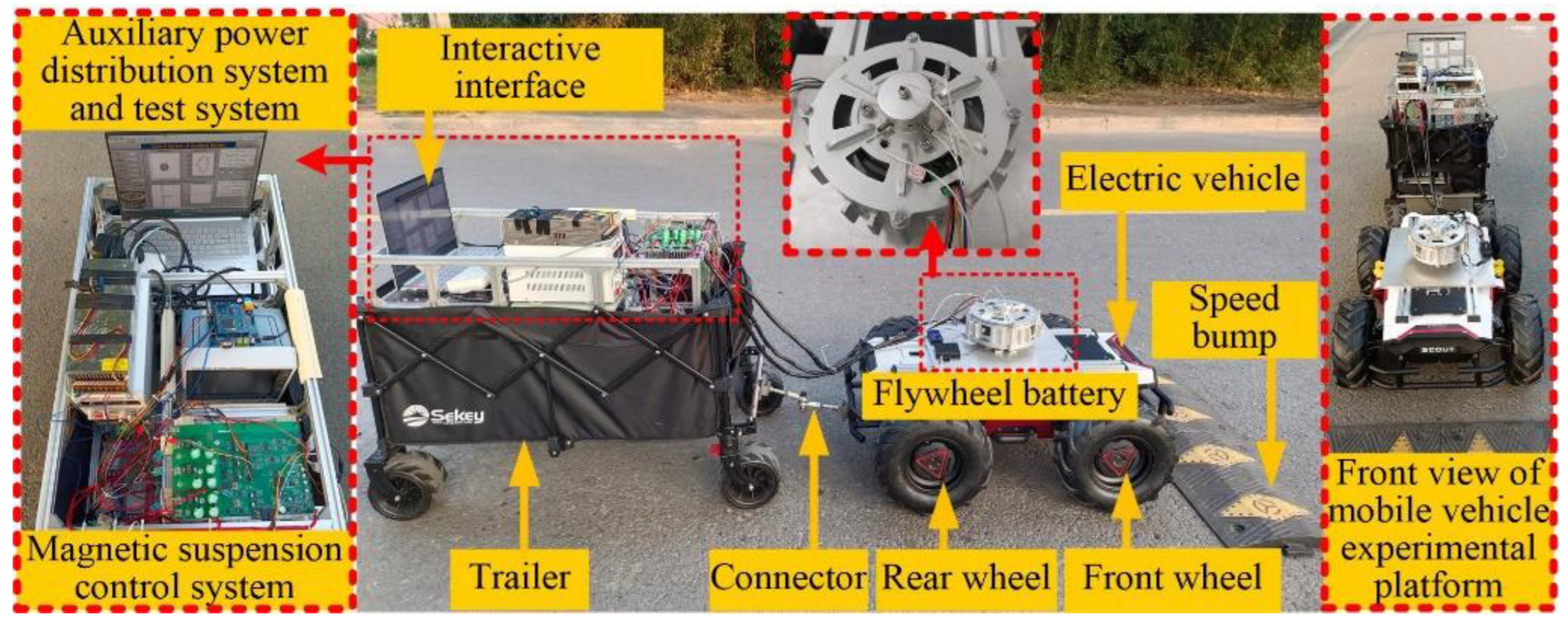
The overall mobile vehicle experimental platform is shown in Figure 18. The experimental platform is mainly composed of an electric vehicle, a flywheel battery system, a magnetic suspension control system, an auxiliary power distribution system, and a test system. The flywheel battery system is vertically installed on the electric vehicle to simulate the working situation of the vehicle-mounted flywheel battery system so as to better verify the proposed theoretical analysis. The vehicle is connected to a trailer carrying magnetic suspension control system, auxiliary power distribution system, and test system using a specially made connector. The connector not only enables 360-degree rotation but also enables the electric vehicle in front of a sudden brake; thus, the rear trailer will not have an inertial impact on the electric vehicle in front. The real-time displacement data of the flywheel battery is transmitted to the rear control system using the line for processing. It can be seen that the real-time interactive interface based on LABVIEW software can reflect the implementation and running state of the flywheel battery at any time and can also change the parameters of the PID controller with the interface at any time. In addition, the classical PID controller based on the proposed parameter control adjustment algorithm is used in the magnetic suspension control system to improve the control efficiency and accuracy.
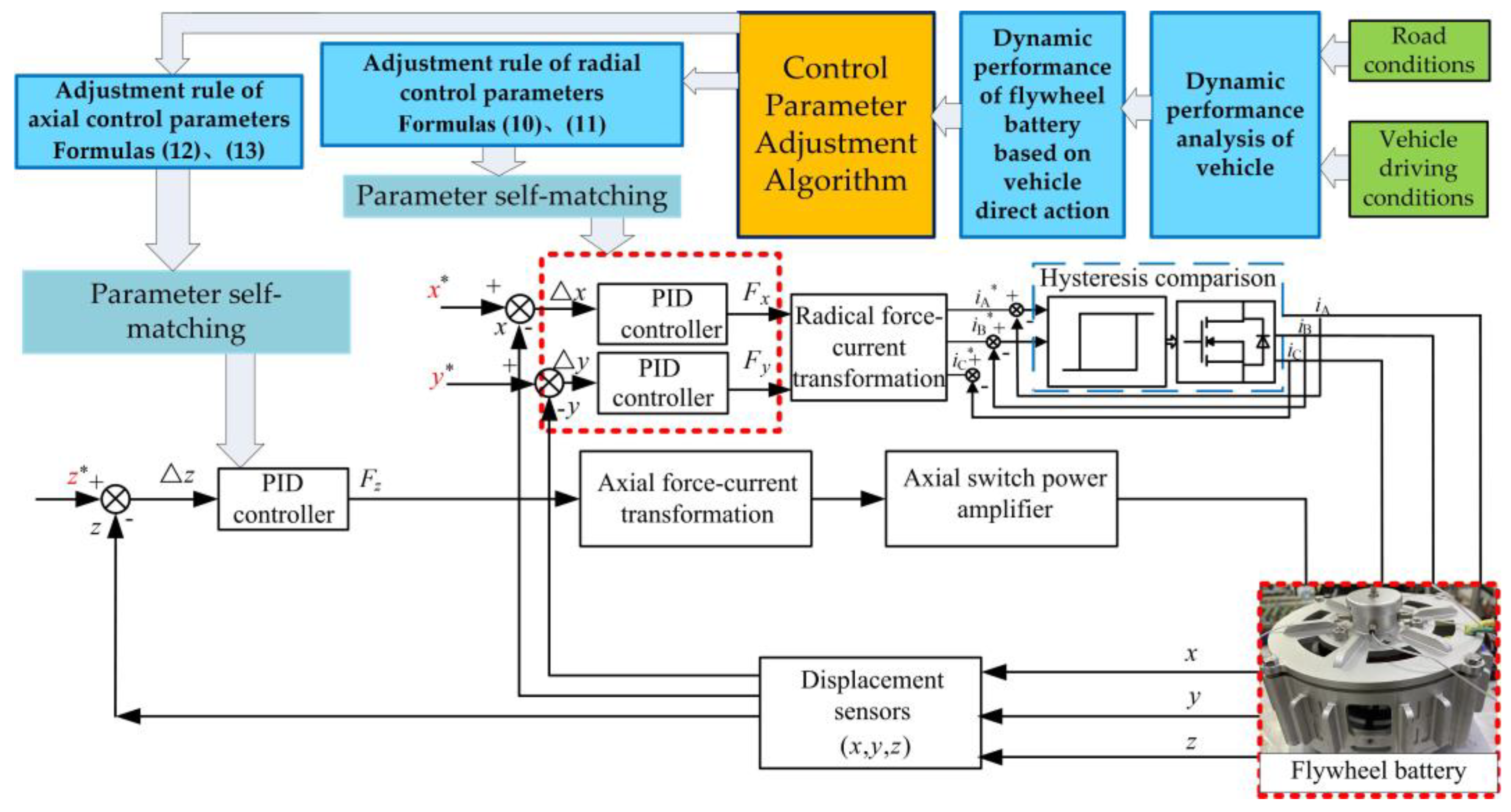
The overall control block diagram based on the dynamic performance analysis results and parameter adjustment algorithm proposed in this study is shown in Figure 19. The magnetic suspension control system includes dynamic performance analysis modules under the influence of typical road conditions and vehicle driving conditions and the control parameter adjustment algorithm module, PID controller setting module, force–current conversion module, current hysteresis comparison module, and displacement measurement module. According to the dynamic performance analysis law of different vehicle speeds over speed bumps, the corresponding control parameter adjustment algorithm can be obtained by summarizing the law. Then, the controller parameter adjustment method is written into the program for the magnetic control system as “expert experience” to guide the real-time self-matching of the PID controller parameters.
The specific steps are described by the accurate dynamic performance analysis used in this study, that is, the model is first modeled according to the steps shown in Figure 1. The model includes a flywheel battery body model and external condition model. Then, the dynamic performance analysis of the vehicle under road conditions and vehicle driving conditions can be carried out in combination with the process in Figure 1. Further, the dynamic performance of the flywheel battery under the direct action of the vehicle are analyzed. Then, based on the above analysis methods and results, the curve fitting method is used to find the dynamic performance response of the flywheel under different PID control parameters. Finally, according to the rules of PID controller parameter adjustment under the influence of specific vehicle driving conditions and road conditions, the algorithm is applied to the magnetic suspension control system program so that the PID controller parameter self-matching can be realized and the high stability of the vehicle flywheel battery can be realized.
4.2. Performance Tests
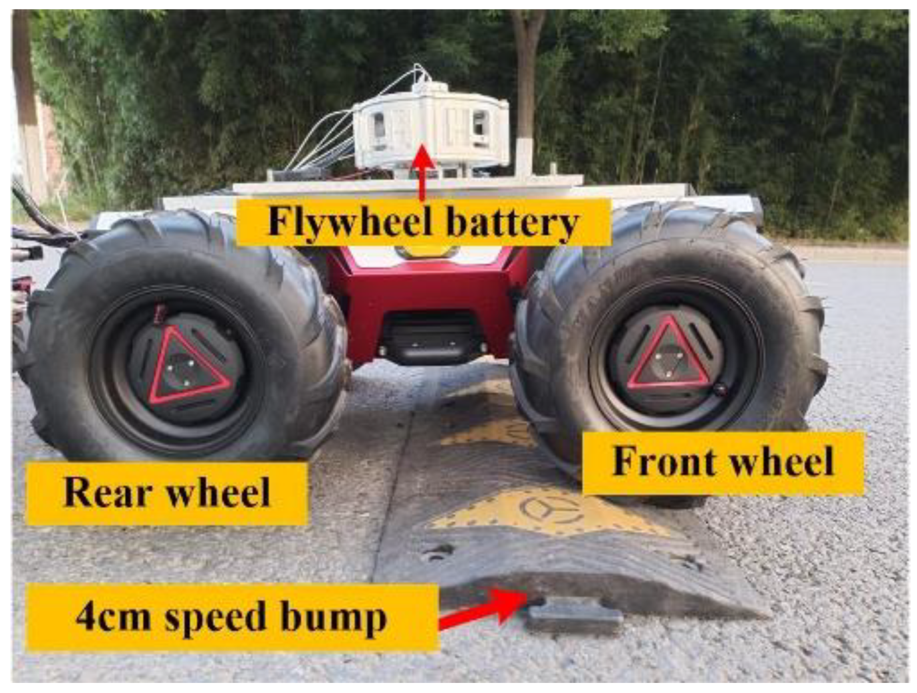
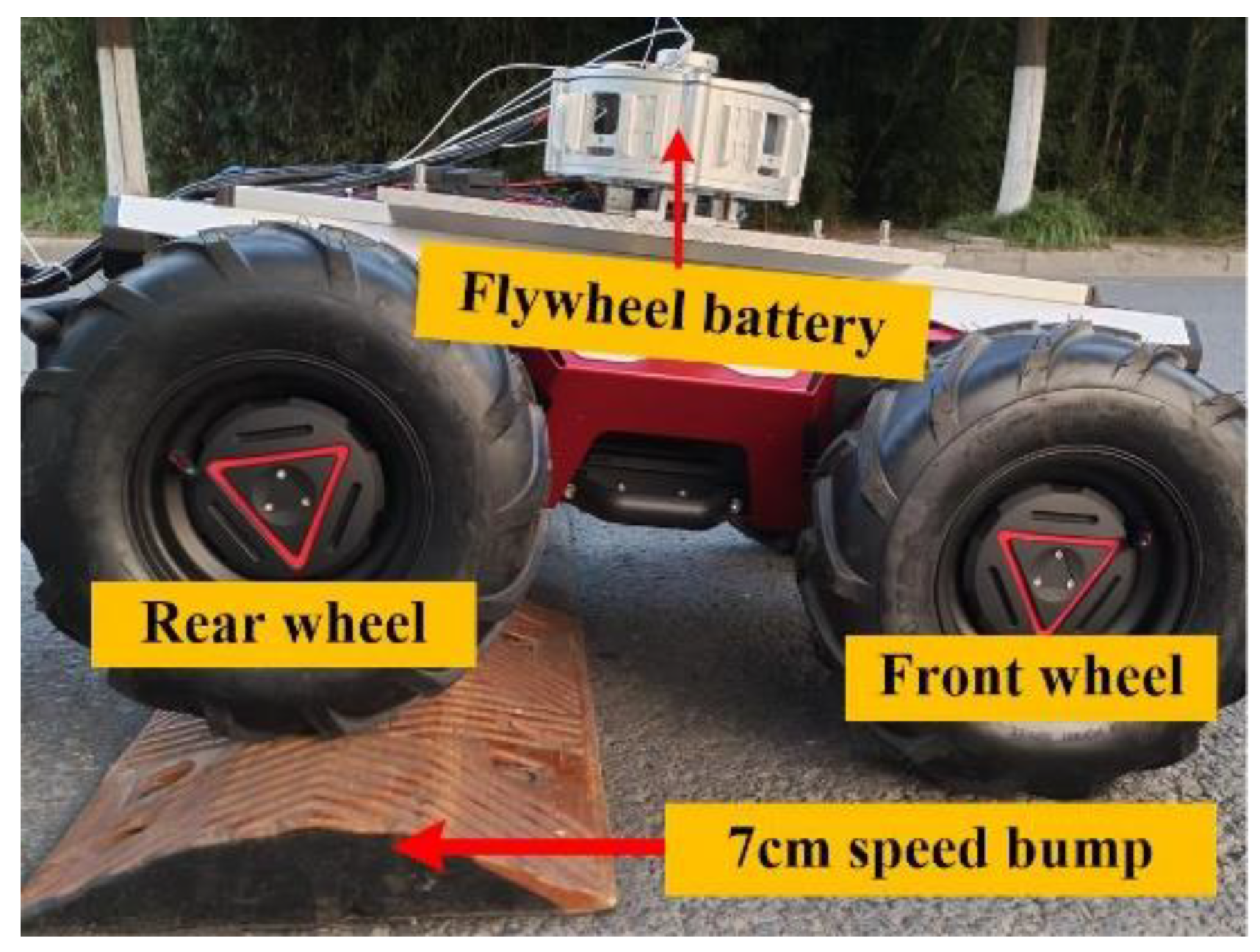
To verify the correctness of the above theoretical analysis results, experiments are performed using vehicles crossing over speed bumps at different speeds. The vehicle speeds are set at 0.7 m/s (2.5 km/h), 0.8 m/s, and 1 m/s. Figure 20 and Figure 21 show the process of the electric vehicle passing over 4 cm and 7 cm speed bumps. The specific parameters of the speed bumps are shown in Table 3, and the wheelbase of the vehicle is 50 cm.
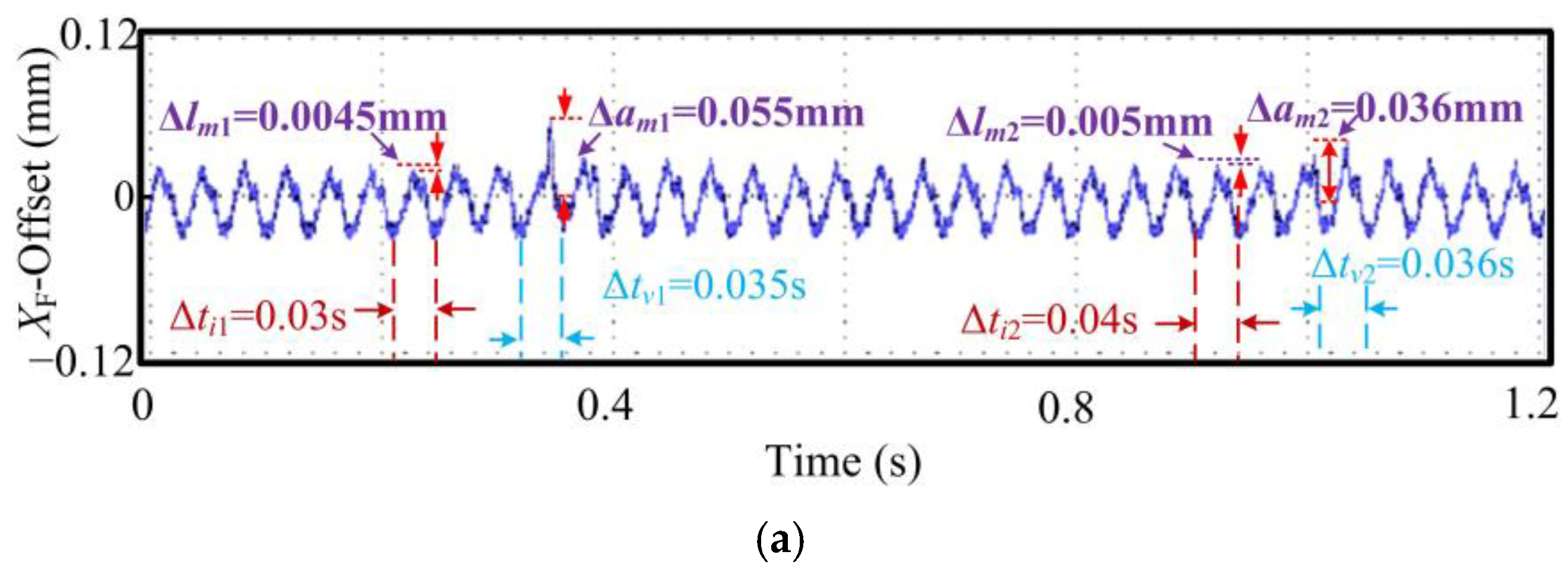
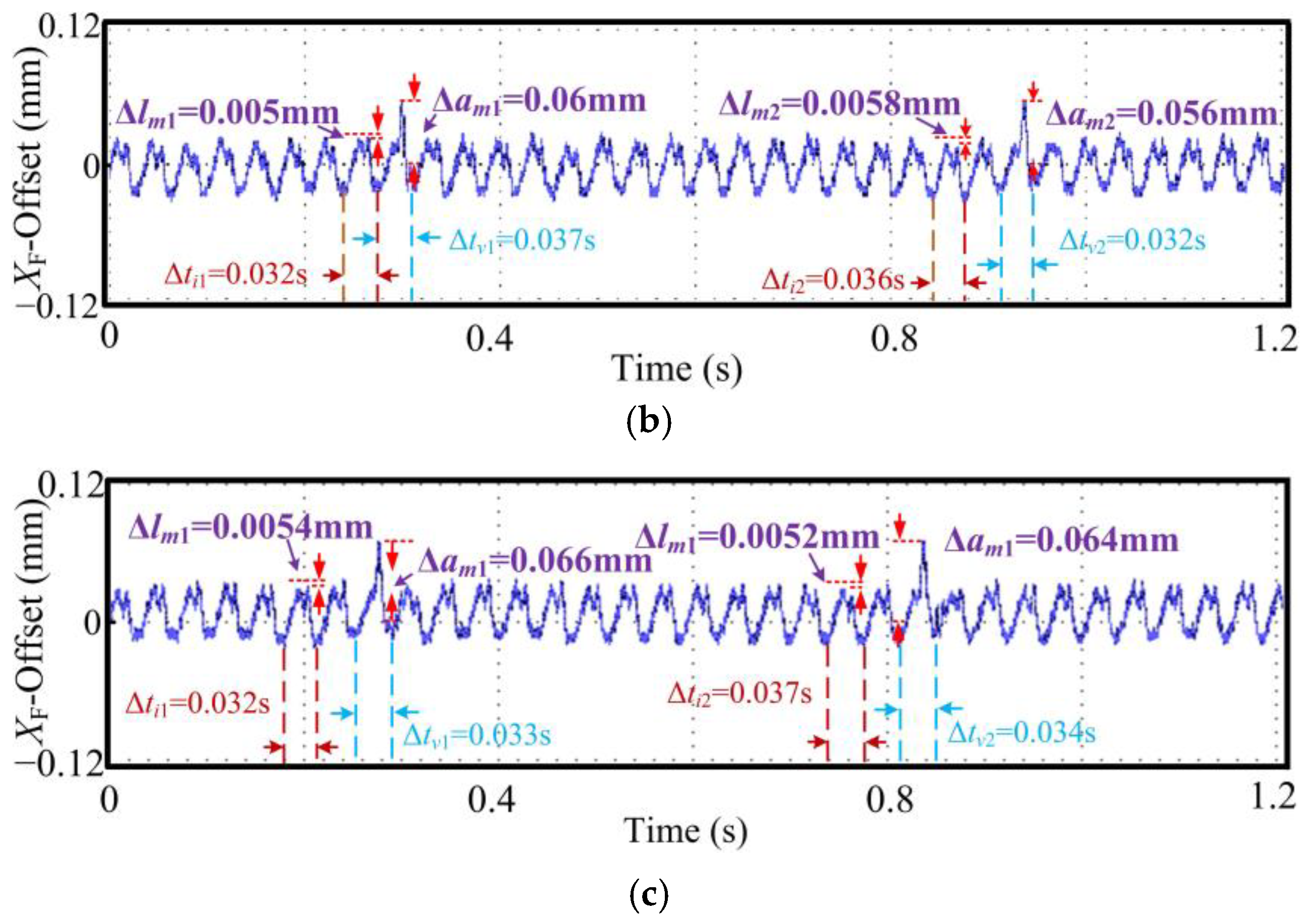
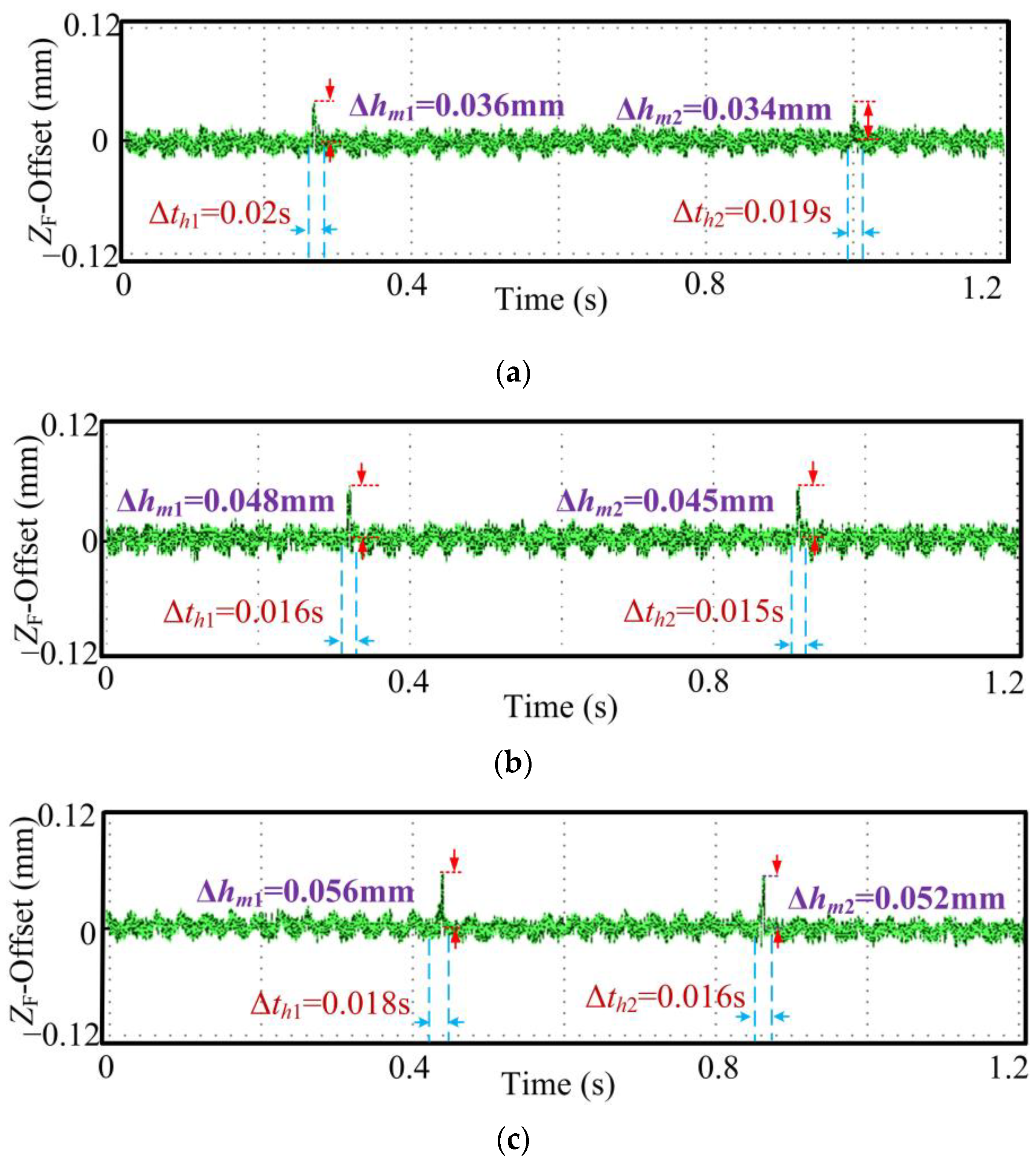
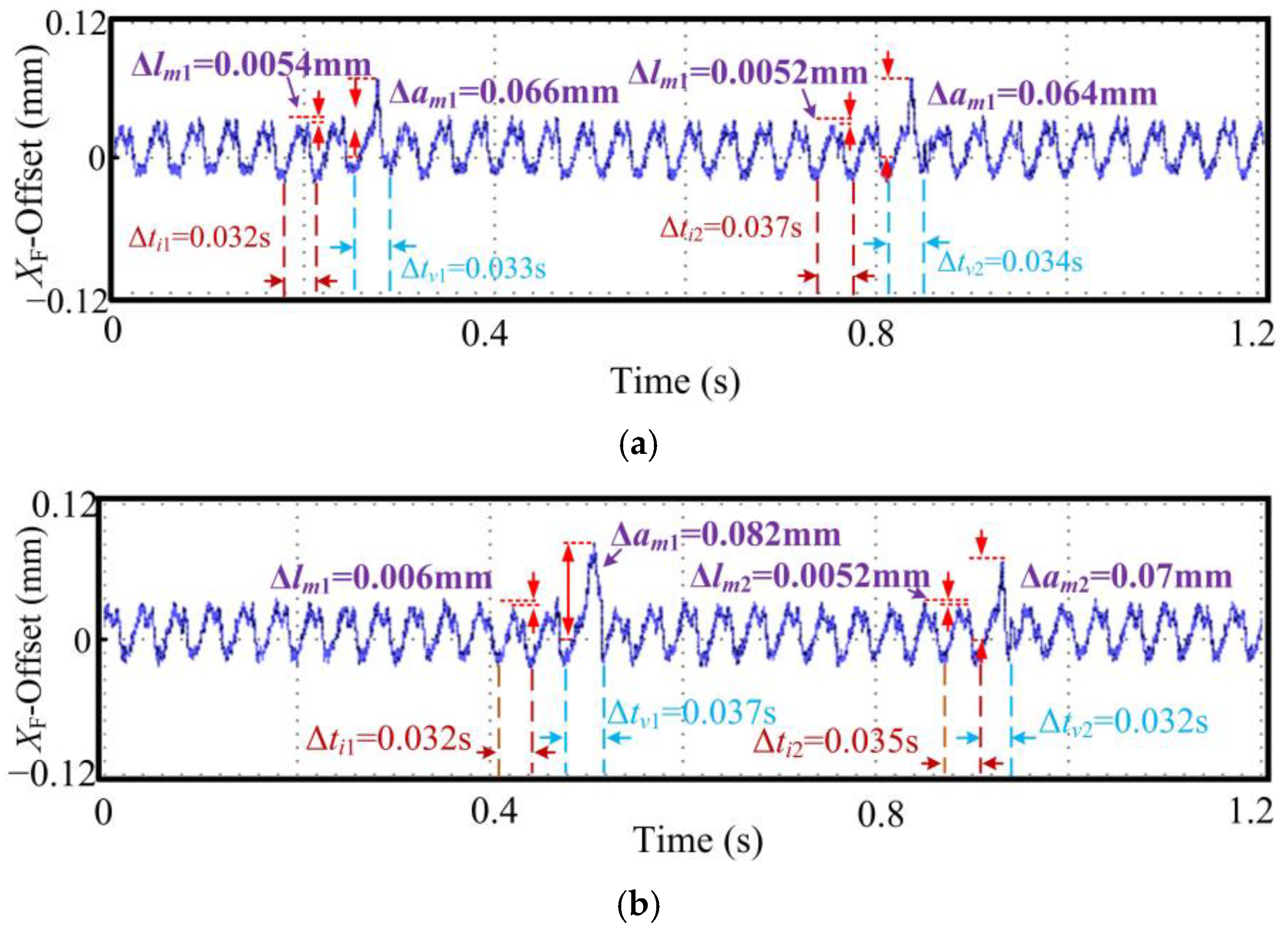
Regarding the experiment with a 4 cm speed bump, the dynamic performance results for the flywheel when the vehicle passes over the speed bump at different speeds are shown in Figure 22 and Figure 23. These results are based on the radial and axial parameter adjustment laws proposed in Equations (10)–(13).
In order to better observe the dynamic performance details of the flywheel when the front wheel and the rear wheel, respectively, pass over the speed bump, the waveform is analyzed in detail in this paper, so some key variables are named as follows: ① the maximum lag variation in the flywheel impacted by the front and rear wheels in the radial direction (focusing on the XF direction of the flywheel battery, as an example) is Δlm1 and Δlm2, respectively, and the adjustment time is Δti1 and Δti2, respectively. ② The maximum upward variation in the flywheel caused by the subsequent two shocks is Δam1 and Δam2, respectively, and the adjustment time is Δtv1 and Δtv2, respectively. ③ In the axial ZF direction of the flywheel battery, the flywheel is subjected to impact and vibration lead changes in the front and rear wheels by Δhm1 and Δhm2, respectively, and the adjustment time is Δth1 and Δth2, respectively.
The control process for the control parameters corresponding to the above three speeds is consistent with the simulation trend in Figure 7 and Figure 9 when going up the slope and when reaching the highest point of the speed bump. However, since the suspension and mass parameters of the experimental vehicle differ from those of the simulated vehicle by orders of magnitude, the hysteresis perturbation is not obvious when the vehicle rushes down from the speed bump and is pulled back to the equilibrium position under the action of the control system. Thus, the experimental results show that the flywheel can quickly return to the equilibrium position under the regulation of the control parameters proposed in this paper. Therefore, it is proved that the proposed method can ensure that the flywheel can run stably under the influence of speed and the speed bumps.
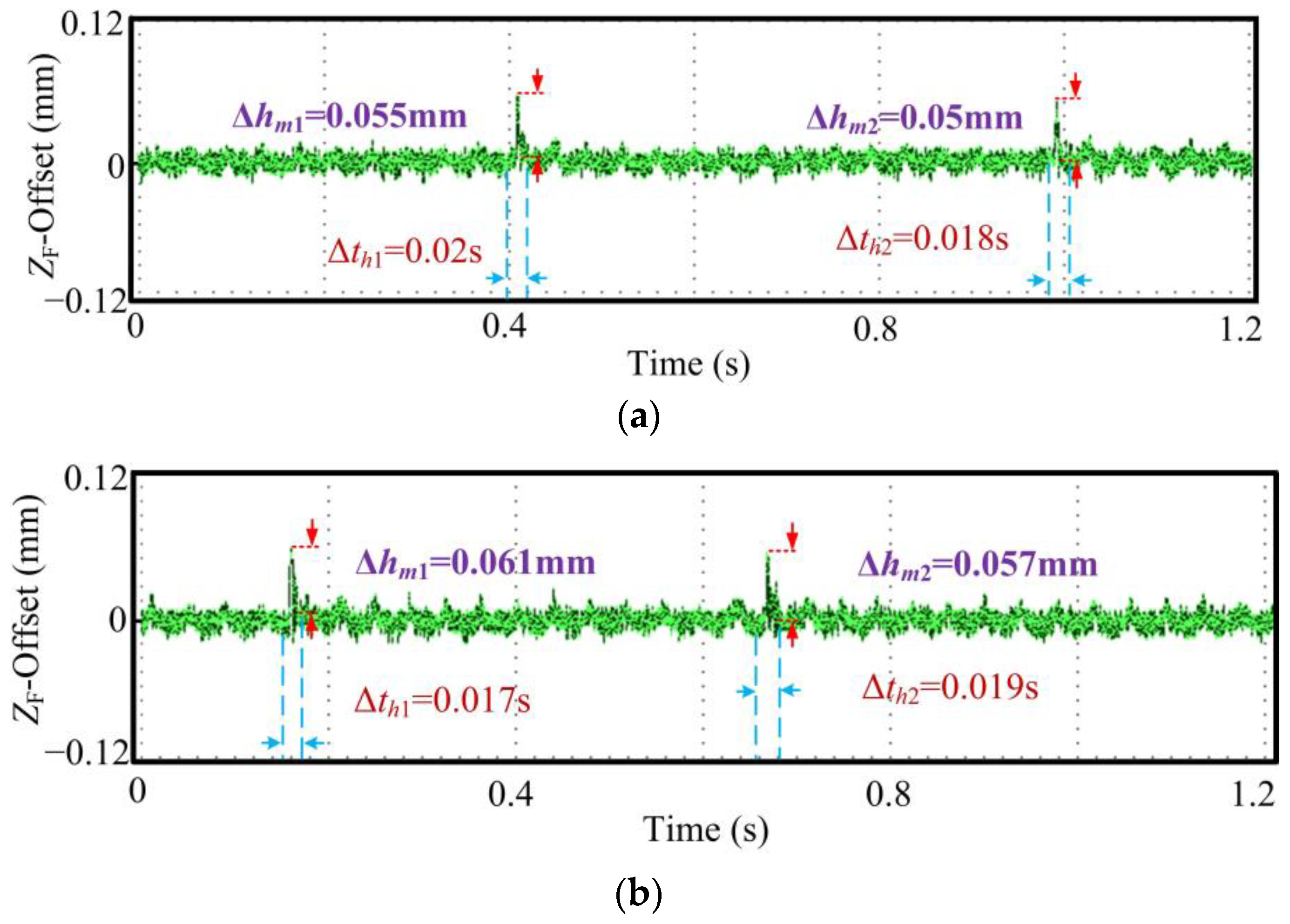
In addition, for the experiments with a 7 cm speed bump, vehicle speeds of 0.8 m/s and 1 m/s are chosen. The results for the dynamic performance of the flywheel with the adjustment algorithm in the respective directions are shown in Figure 24 and Figure 25. It is particularly noted that as the height of the speed bump increases, the corresponding shock and vibration processes also increase. Again, good experimental results show that the flywheel is able to quickly return to its equilibrium position while also effectively reducing the effects of disturbances. Thus, it is demonstrated that the proposed method is able to ensure the stable operation of the flywheel despite the effects of higher bumps at vehicle speed and height.
5. Conclusions
Traditional methods often overlook the direct impact of vehicle vibration on the flywheel battery system, resulting in an inaccurate analysis of the dynamic performance and control effectiveness of the flywheel battery system. Therefore, in order to make up for the shortcomings of existing research, this study proposes a more accurate dynamic performance analysis method and an efficient control parameter adjustment algorithm for flywheel batteries based on the direct action of vehicles. When considering the dynamic performance of a vehicle-mounted flywheel battery under the influence of road and vehicle driving conditions, this study first analyzes the impact of road conditions and vehicle driving conditions on vehicle stability. Then, the vibration signals generated by the vehicle are transmitted to the magnetic flywheel battery system for precise analysis to ensure the accuracy of the analysis. Then, according to the stability analysis results of the direct action of the vehicle, based on the classical practical PID controller, the control parameter adjustment algorithm is summarized using the curve fitting method. The proposed algorithm can respond quickly and accurately and restrain external excitation more effectively, which improves the engineering practicability of the control parameter adjustment algorithm. Finally, a performance test is carried out on the designed mobile vehicle experimental platform. Good experimental results verify the correctness of the proposed theory and algorithm.
In addition, it is worth noting that the method proposed in this paper is universal. This paper takes into account the actual working conditions of the most common urban speed bump of 4 cm or more when deriving the formula. If there are special circumstances, such as a speed bump less than 4 cm, then it is completely possible to write the general formula of the PID controller parameters for the speed bump less than 4 cm in height according to the derivation formula and curve fitting method proposed in this paper.
Moreover, it is worth noting that only very common and extreme representatives of road conditions and vehicle driving conditions are selected for analysis in this paper. Therefore, according to the analysis ideas in this paper, more comprehensive conditions can be analyzed in the future, and a more comprehensive control parameter adjustment algorithm can be summarized.
Author Contributions
Project administration, W.Z.; Writing—original draft, J.C.; Conceptualization, W.Z.; methodology, J.C.; software, J.C.; validation, J.C. and W.Z. All authors have read and agreed to the published version of the manuscript.
Funding
This work was supported in part by the National Natural Science Foundation of China under Grant 52077099, and in part by the China Postdoctoral Science Foundation under Grant 2019M651737.
Data Availability Statement
Not applicable.
Conflicts of Interest
The authors declare no conflict of interest.
References
- Bianchini, C.; Torreggiani, A.; David, D.; Bellini, A. Design of motor/generator for flywheel batteries. IEEE Trans. Ind. Electron. 2021, 68, 9675–9684. [Google Scholar] [CrossRef]
- Li, X.J.; Palazzolo, A.; Wang, Z.Y. A combination 5-DOF active magnetic bearing for energy storage flywheels. IEEE Trans. Transp. Electrif. 2021, 7, 2344–2355. [Google Scholar] [CrossRef]
- Zhang, W.Y.; Wang, Z. Dual mode coordinated control of magnetic suspension flywheel battery based on vehicle driving conditions characteristics. IEEE Trans. Ind. Electron. 2023. Early Access. [Google Scholar] [CrossRef]
- Motaman, S.; Eltaweel, M.; Herfatmanesh, M.R.; Knichel, T.; Deakin, A. Numerical analysis of a flywheel energy storage system for low carbon powertrain applications. J. Energy Storage 2023, 61, 106808. [Google Scholar] [CrossRef]
- Zhong, B.F.; Li, J.L.; Cai, X.J.; Chen, T.; An, Q.L.; Chen, M. Structural design optimization of CFRP/Al hybrid co-cured high-speed flywheel with the particle swarm optimization algorithm. Polym. Compos. 2023, 44, 2161–2172. [Google Scholar] [CrossRef]
- Deng, Y.; Zhao, Y.; Pi, W.; Li, Y.; Feng, S.; Du, Y. The influence of nonlinear stiffness of novel flexible road wheel on ride comfort of tracked vehicle traversing random uneven road. IEEE Access 2019, 7, 165293–165302. [Google Scholar] [CrossRef]
- Sun, M.L.; Zheng, S.Q.; Wang, K.; Zheng, S.Q.; Wang, K.; Le, Y. Filter cross-feedback control for nutation mode of asymmetric rotors with gyroscopic effects. IEEE/ASME Trans. Mechatron. 2020, 25, 248–258. [Google Scholar] [CrossRef]
- Zheng, S.Q.; Yang, J.Y.; Song, X.D.; Ma, C. Tracking compensation control for nutation mode of high-speed rotors with strong gyroscopic effects. IEEE Trans. Ind. Electron. 2018, 65, 4156–4165. [Google Scholar] [CrossRef]
- Han, B.C.; Chen, Y.L.; Zheng, S.Q.; Li, M.X.; Xie, J.J. Whirl mode suppression for AMB-rotor systems in control moment gyros considering significant gyroscopic effects. IEEE Trans. Ind. Electron. 2021, 68, 4249–4258. [Google Scholar] [CrossRef]
- Zhang, L.J.; Du, B.; Feng, J. Control for the magnetically suspended flat rotor tilting by axial forces in a small-scale control moment gyro. IEEE Trans. Ind. Electron. 2018, 65, 2449–2457. [Google Scholar] [CrossRef]
- Ding, G.P.; Zhou, Z.D.; Hu, Y.F. Test of base vibration influence on dynamics of a magnetic suspended disk. In Proceedings of the 2008 IEEE/ASME International Conference Advanced Intelligent Mechatronics, Xi’an, China, 2–5 July 2008; pp. 308–313. [Google Scholar]
- Zhang, W.Y.; Zhang, L.D.; Li, K.; Zhu, H.Q. Dynamic correction model considering influence of foundation motions for a centripetal force type-magnetic bearing. IEEE Trans. Ind. Electron. 2021, 68, 9811–9821. [Google Scholar] [CrossRef]
- Zhang, W.Y.; Zhu, P.F.; Wang, J.P.; Zhu, H.Q. Stability control for a centripetal force type-magnetic bearing-rotor system based on golden frequency section point. IEEE Trans. Ind. Electron. 2021, 68, 12482–12492. [Google Scholar] [CrossRef]
- Itani, K.; De Bernardinis, A.; Khatir, Z.; Jammal, A. Integration of different modules of an electric vehicle powered by a battery-flywheel storage system during traction operation. In Proceedings of the 2016 IEEE International Multidisciplinary Conference on Engineering Technology, Beirut, Lebanon, 4 February 2016; pp. 126–131. [Google Scholar]
- Soni, T.; Sodhi, R. Impact of harmonic road disturbances on active magnetic bearing supported flywheel energy storage system in electric vehicles. In Proceedings of the 2019 IEEE Transportation Electrification Conference (ITEC-India), Bengaluru, India, 17–19 December 2019; pp. 1–4. [Google Scholar]
- Kasarda, M.E.; Clements, J.; Wicks, A.L.; Hall, C.D.; Kirk, R.G. Effect of sinusoidal base motion on a magnetic bearing. In Proceedings of the 2000 IEEE International Conference on Control Applications, Anchorage, AK, USA, 27 September 2000; pp. 144–149. [Google Scholar]
- Sun, Y.G.; Xu, J.Q.; Wu, H.; Lin, G.B.; Shahid, M. Deep learning based semi-supervised control for vertical security of maglev vehicle with guaranteed bounded airgap. IEEE Trans. Intell. Transp. Syst. 2021, 22, 4431–4442. [Google Scholar] [CrossRef]
- Sun, Y.G.; Xu, J.Q.; Chen, C.; Hu, W. Reinforcement learning-based optimal tracking control for levitation system of maglev vehicle with input time delay. IEEE Trans. Instrum. Meas. 2022, 71, 7500813. [Google Scholar] [CrossRef]
- Zhang, W.Y.; Wang, J.P.; Zhu, P.F.; Yu, J.X. A novel vehicle-mounted magnetic suspension flywheel battery with a virtual inertia spindle. IEEE Trans. Ind. Electron. 2022, 69, 5973–5983. [Google Scholar] [CrossRef]
Figure 1.
Flow chart showing the dynamic performance analysis.

Figure 2.
Lateral displacement of a vehicle’s body as it passes over a speed bump. (a) Vehicle speed of 10 km/h. (b) Vehicle speed of 20 km/h.
Figure 2.
Lateral displacement of a vehicle’s body as it passes over a speed bump. (a) Vehicle speed of 10 km/h. (b) Vehicle speed of 20 km/h.

Figure 3.
Impact acceleration of a vehicle when the vehicle speed is 20 km/h. (a) In the XC direction. (b) In the ZC direction.
Figure 3.
Impact acceleration of a vehicle when the vehicle speed is 20 km/h. (a) In the XC direction. (b) In the ZC direction.

Figure 4.
Comparison of body acceleration under front wheel excitation at different speeds. (a) In the XC direction. (b) In the ZC direction.
Figure 4.
Comparison of body acceleration under front wheel excitation at different speeds. (a) In the XC direction. (b) In the ZC direction.

Figure 5.
Control block diagram using the classical PID controller and ADAMS co-simulation.

Figure 6.
Dynamic performance of a flywheel in the XF direction without a magnetic suspension control system. (a) The vehicle speed is 2.5 km/h. (b) The vehicle speed is 10 km/h. (c) The vehicle speed is 20 km/h.
Figure 6.
Dynamic performance of a flywheel in the XF direction without a magnetic suspension control system. (a) The vehicle speed is 2.5 km/h. (b) The vehicle speed is 10 km/h. (c) The vehicle speed is 20 km/h.

Figure 7.
Dynamic performance of a flywheel in the XF direction with a magnetic suspension control system. (a) The vehicle speed is 2.5 km/h. (b) The vehicle speed is 10 km/h. (c) The vehicle speed is 20 km/h.
Figure 7.
Dynamic performance of a flywheel in the XF direction with a magnetic suspension control system. (a) The vehicle speed is 2.5 km/h. (b) The vehicle speed is 10 km/h. (c) The vehicle speed is 20 km/h.

Figure 8.
Dynamic performance of a flywheel in the ZF direction without a magnetic suspension control system. (a) The vehicle speed is 2.5 km/h. (b) The vehicle speed is 10 km/h. (c) The vehicle speed is 20 km/h.
Figure 8.
Dynamic performance of a flywheel in the ZF direction without a magnetic suspension control system. (a) The vehicle speed is 2.5 km/h. (b) The vehicle speed is 10 km/h. (c) The vehicle speed is 20 km/h.

Figure 9.
Dynamic performance of a flywheel in the ZF direction with a magnetic suspension control system. (a) The vehicle speed is 2.5 km/h. (b) The vehicle speed is 10 km/h. (c) The vehicle speed is 20 km/h.
Figure 9.
Dynamic performance of a flywheel in the ZF direction with a magnetic suspension control system. (a) The vehicle speed is 2.5 km/h. (b) The vehicle speed is 10 km/h. (c) The vehicle speed is 20 km/h.


Figure 10.
Fitting results for the radial control parameters and vehicle speeds when the vehicle passes over a 4 cm speed bump. (a) Proportional parameters and vehicle speeds. (b) Derivative parameters and vehicle speeds.
Figure 10.
Fitting results for the radial control parameters and vehicle speeds when the vehicle passes over a 4 cm speed bump. (a) Proportional parameters and vehicle speeds. (b) Derivative parameters and vehicle speeds.

Figure 11.
Radial dynamic performance of the flywheel with a control parameter adjustment algorithm. (a) Vehicle speed of 16 km/h. (b) Vehicle speed of 22 km/h.
Figure 11.
Radial dynamic performance of the flywheel with a control parameter adjustment algorithm. (a) Vehicle speed of 16 km/h. (b) Vehicle speed of 22 km/h.

Figure 12.
Fitting results for the axial control parameters and vehicle speeds when the vehicle passes over a 4 cm speed bump. (a) Proportional parameters and vehicle speeds. (b) Derivative parameters and vehicle speeds.
Figure 12.
Fitting results for the axial control parameters and vehicle speeds when the vehicle passes over a 4 cm speed bump. (a) Proportional parameters and vehicle speeds. (b) Derivative parameters and vehicle speeds.

Figure 13.
Axial dynamic performance of the flywheel with a control parameter adjustment algorithm. (a) Vehicle speed of 16 km/h. (b) Vehicle speed of 22 km/h.
Figure 13.
Axial dynamic performance of the flywheel with a control parameter adjustment algorithm. (a) Vehicle speed of 16 km/h. (b) Vehicle speed of 22 km/h.

Figure 14.
Radial dynamic performance of the flywheel at a vehicle speed of 10 km/h in the case when the vehicle passes over a 7 cm speed bump. (a) Without the controller. (b) With the controller.
Figure 14.
Radial dynamic performance of the flywheel at a vehicle speed of 10 km/h in the case when the vehicle passes over a 7 cm speed bump. (a) Without the controller. (b) With the controller.

Figure 15.
Axial dynamic performance of the flywheel at a vehicle speed of 10 km/h in the case when the vehicle passes over a 7 cm speed bump. (a) Without the controller. (b) With the controller.
Figure 15.
Axial dynamic performance of the flywheel at a vehicle speed of 10 km/h in the case when the vehicle passes over a 7 cm speed bump. (a) Without the controller. (b) With the controller.

Figure 16.
Fitting results for the radial control parameters and vehicle speeds when a vehicle passes over the 7 cm speed bump. (a) Proportional parameters and vehicle speeds. (b) Derivative parameters and vehicle speeds.
Figure 16.
Fitting results for the radial control parameters and vehicle speeds when a vehicle passes over the 7 cm speed bump. (a) Proportional parameters and vehicle speeds. (b) Derivative parameters and vehicle speeds.

Figure 17.
Fitting results for the axial control parameters and vehicle speeds when a vehicle passes over the 7 cm speed bump. (a) Proportional parameters and vehicle speeds. (b) Derivative parameters and vehicle speeds.
Figure 17.
Fitting results for the axial control parameters and vehicle speeds when a vehicle passes over the 7 cm speed bump. (a) Proportional parameters and vehicle speeds. (b) Derivative parameters and vehicle speeds.

Figure 18.
The mobile experimental platform.

Figure 19.
Overall control block diagram.

Figure 20.
The vehicle passes over a 4 cm speed bump.

Figure 21.
The vehicle passes over a 7 cm speed bump.

Figure 22.
Radial dynamic performance of the flywheel at different vehicle speeds when the vehicle passes over a 4 cm speed bump. (a) Vehicle speed of 0.7 m/s. (b) Vehicle speed of 0.8 m/s. (c) Vehicle speed of 1 m/s.
Figure 22.
Radial dynamic performance of the flywheel at different vehicle speeds when the vehicle passes over a 4 cm speed bump. (a) Vehicle speed of 0.7 m/s. (b) Vehicle speed of 0.8 m/s. (c) Vehicle speed of 1 m/s.


Figure 23.
Axial dynamic performance of the flywheel at different vehicle speeds when the vehicle passes over a 4 cm speed bump. (a) Vehicle speed of 0.7 m/s. (b) Vehicle speed of 0.8 m/s. (c) Vehicle speed of 1 m/s.
Figure 23.
Axial dynamic performance of the flywheel at different vehicle speeds when the vehicle passes over a 4 cm speed bump. (a) Vehicle speed of 0.7 m/s. (b) Vehicle speed of 0.8 m/s. (c) Vehicle speed of 1 m/s.

Figure 24.
Radial dynamic performance of the flywheel at different vehicle speeds when the vehicle passes over a 7 cm speed bump. (a) Vehicle speed of 0.8 m/s. (b) Vehicle speed of 1 m/s.
Figure 24.
Radial dynamic performance of the flywheel at different vehicle speeds when the vehicle passes over a 7 cm speed bump. (a) Vehicle speed of 0.8 m/s. (b) Vehicle speed of 1 m/s.

Figure 25.
Axial dynamic performance of the flywheel at different vehicle speeds when the vehicle passes over a 7 cm speed bump. (a) Vehicle speed of 0.8 m/s. (b) Vehicle speed of 1 m/s.
Figure 25.
Axial dynamic performance of the flywheel at different vehicle speeds when the vehicle passes over a 7 cm speed bump. (a) Vehicle speed of 0.8 m/s. (b) Vehicle speed of 1 m/s.


Table 1.
Key technical parameters of the flywheel battery.
| Specification | Value |
|---|---|
| Maximum mass energy density | 6.4 Wh/kg |
| Energy storage | 6.5 Wh |
| Maximum speed of the flywheel | 15,000 r/min |
| Diameter of the flywheel | 37 mm |
| Mass of the flywheel | 2.8 kg |
Table 2.
Key parameters of the vehicle.
| Parameter | Value |
|---|---|
| Mass | 1527 kg |
| Front suspension spring stiffness | 31 N/mm |
| Rear suspension spring stiffness | 37 N/mm |
| Front wheelbase | 1500 mm |
| Rear wheelbase | 1520 mm |
| Wheelbase | 2560 mm |
Table 3.
Specific structural parameters of the speed bumps.
| Height | Length | Width | Slope Length |
|---|---|---|---|
| 4 cm | 33.5 cm | 98 cm | 17.5 cm |
| 7 cm | 34 cm | 98 cm | 18.5 cm |
Disclaimer/Publisher’s Note: The statements, opinions and data contained in all publications are solely those of the individual author(s) and contributor(s) and not of MDPI and/or the editor(s). MDPI and/or the editor(s) disclaim responsibility for any injury to people or property resulting from any ideas, methods, instructions or products referred to in the content. |
© 2023 by the authors. Licensee MDPI, Basel, Switzerland. This article is an open access article distributed under the terms and conditions of the Creative Commons Attribution (CC BY) license (https://creativecommons.org/licenses/by/4.0/).
Share and Cite
MDPI and ACS Style
Zhang, W.; Cui, J. Dynamic Performance Analysis and Control Parameter Adjustment Algorithm for Flywheel Batteries Considering Vehicle Direct Action. Energies 2023, 16, 5882. https://0-doi-org.brum.beds.ac.uk/10.3390/en16165882
AMA Style
Zhang W, Cui J. Dynamic Performance Analysis and Control Parameter Adjustment Algorithm for Flywheel Batteries Considering Vehicle Direct Action. Energies. 2023; 16(16):5882. https://0-doi-org.brum.beds.ac.uk/10.3390/en16165882
Chicago/Turabian StyleZhang, Weiyu, and Junjie Cui. 2023. "Dynamic Performance Analysis and Control Parameter Adjustment Algorithm for Flywheel Batteries Considering Vehicle Direct Action" Energies 16, no. 16: 5882. https://0-doi-org.brum.beds.ac.uk/10.3390/en16165882
Note that from the first issue of 2016, this journal uses article numbers instead of page numbers. See further details here.