An Automatic Apparatus for Simultaneous Measurement of Seebeck Coefficient and Electrical Resistivity

Abstract

A fully automated experimental system was designed for simultaneous measurement of the Seebeck coefficient and electrical resistivity of thermoelectric materials in bulk form. The system incorporates a straightforward and easily fabricated sample holder along with commercially available electronic instrument components. The sample holder showcases a compact design that utilizes two Peltier module heaters to induce sample heating and generate the required temperature gradient. System automation and control are achieved through the implementation of a LabView program. The Seebeck voltage and resistance of the sample (under specified temperature conditions) are determined using I–V measurements. The Seebeck voltage and resistance of the sample correspond to the intercept and slope of the I–V characteristic diagram in the four-point probe method, respectively. To verify the accuracy and reliability of the developed apparatus, a variety of experiments were performed on N-type and P-type bismuth telluride samples. The measurement results closely matched those obtained from commercial systems, with an overall data difference of less than 10% for both the Seebeck coefficient and resistivity measurements.

1. Introduction

The thermoelectric effect refers to the direct conversion of temperature differences into electrical voltage, and vice versa. This phenomenon arises from the movement of charge carriers within the thermoelectric material [1]. The Seebeck coefficient (S) is a key parameter to evaluate this heat-to-electricity conversion in thermoelectric materials. It quantifies the relationship between the generated voltage (ΔV) and a given temperature difference (ΔT) as $S=-\Delta V/\Delta T$. It is dependent on the concentration, mobility, and conduction mechanism of charge carriers [2]. In thermoelectric devices, the performance of thermoelectric materials is characterized by a dimensionless figure of merit ZT, as $ZT=\frac{S^2}{\rho \kappa }T$ [3], in which $\rho$, $\kappa$, and T represent the resistivity, thermal conductivity, and absolute temperature, respectively. The Seebeck coefficient and resistivity not only describe the fundamental transport properties of electrons but also serve as key performance indicators for thermoelectric materials. Therefore, facile and precise measurement of S and $\rho$ is essential for practical applications of thermoelectric materials.

The measurement process for the Seebeck coefficient (S) and resistivity ($\rho$) can be discussed in terms of four key aspects: measurement principle, implementation method, operating parameters, and data acquisition method. The measurement principle involves techniques for measuring the Seebeck voltage (SV) and resistance (R). Various methods have been employed for SV measurement, broadly categorized into two groups: integral methods [4,5] and differential methods [6,7,8]. Differential methods can be further classified based on thermal conditions: steady-state [6], quasi-steady-state [9], and transient [10]. The integral method is suitable for large temperature differences and relatively long, large samples. It involves maintaining one end of the sample at temperature This integration of components is crucial T₁ while heating the other end (possible to use a variety of methods) to generate a temperature difference ΔT across the sample. On the other hand, the differential method is primarily used for small temperature differences and small sample sizes, typically at the laboratory scale [11]. In this method, a small ΔT is applied to the target temperature T, with T_h = T + ΔT/2 and T_c = T − ΔT/2, where T_h and T_c represent the temperature of the hot and cold ends of the sample, respectively. Common resistance measurement methods include the two-probe method [10], four-probe method [6,12], van der Pauw method [13,14], and bridge method [15]. The two-probe method is a simple technique for measuring resistance but is susceptible to issues such as contact resistance between the probes and the sample, as well as the internal resistance of the instrument. In contrast, the four-probe method employs four probes instead of two and separates the roles of current injection and voltage measurement. Two of the probes are specifically employed to apply current to the sample, while the other two are used to measure the voltage across the sample, effectively eliminating the problems encountered in the two-probe method. The van der Pauw method is a more complex technique suitable for samples with irregular shapes or non-uniform conductivity. However, it requires repositioning the probes during the testing process. The bridge method is the most precise and accurate method for measuring resistance, but it requires specialized equipment.

Various implementation methods have been utilized for managing the measurement system, including Python controlling instruments [16], LabVIEW controlling instruments [17], Visual Basics controlling instruments [18], LabVIEW controlling existing instruments and electronic loads [19], and electronic load/circuit [20]. Python is a powerful open-source programming language known for its flexibility and extensive library support, making it suitable for instrument control and integration with data analysis tools. LabVIEW, on the other hand, is a graphical programming language that offers a user-friendly interface for instrument control and can be customized to meet specific experimental requirements. It is particularly useful for real-time data acquisition and control. Visual Basic, developed by Microsoft, is another commonly used programming language for instrument control and data acquisition. It can be seamlessly integrated with other Microsoft products, such as Excel and Access, and it provides advanced data analysis and visualization capabilities. The LabVIEW implementation method for controlling commercial instruments and electronic loads allows for the integration of existing equipment, providing a flexible and customizable interface using LabVIEW, and reducing experimental costs. Lastly, the use of electronic loads or circuits for measuring the Seebeck coefficient and resistivity is suitable for high-precision measurements or experiments involving unique or custom-built electronic circuits.

In all these cases, there are electrical/thermal contacts between the sample and thermocouples, classifiable into three categories: two-point, off-axis four-point, and uniaxial four-point setups [21,22]. The four-point probe method is widely employed for resistivity measurements [23], and maintaining good contact between the sample and thermocouples is crucial. Researchers have explored various techniques to achieve optimal thermal contact, such as drilling small holes in the sample and using highly conductive materials to glue the thermocouples into the holes [4], directly adhering the thermocouples onto the sample surface using silver paste [24], flattening the thermocouple junctions into small disks to increase the contact area [25,26], using beadless thermocouples [13], and applying spring preload to ensure proper contact [27,28,29].

In the next step, accurate and efficient data acquisition is crucial in a reliable measurement system. This process involves collecting, sampling, and processing relevant data from various sensors and instruments. There are different means for temperature acquisition, including thermocouples [30], infrared microscopes [31], resistive sensors [32], and digital temperature sensors [33]. The temperature difference can be then obtained using a differential thermocouple method [34], or by comparing the readings from the two thermocouples [35] or two digital sensors [33]. To measure the Seebeck coefficient and electrical resistance, different techniques have been utilized. For instance, resistance is typically obtained through slope fitting of I–V measurements [36], and to calculate the Seebeck coefficient, the intersection of the fitted line should be recorded [37,38]. To acquire the Seebeck voltage, one can either gather two electrical signals from thermocouples [8] measuring the temperature difference across the sample, or directly measure the electrical leads [18] or connection probes [33] connected to the sample.

After discussing the various methods for measuring the Seebeck coefficient (S) and resistance (R) in thermoelectric materials, it is worth exploring the commercially available solutions. Among them, the ZEM-3 [39], LSR-3 [40], SeebSys [41], and PPMS [42] systems are prominent options for measuring the thermoelectric properties of materials. While they share some similarities in their specifications, there are also differences in the measurement details. In terms of measurement principles, all these systems use the differential method and four-probe method for measuring S and R, respectively [43]. However, the PPMS system offers additional measurement methods such as the van der Pauw method, AC resistance bridge, and two-probe method for resistance measurements [44]. Regarding implementation methods, ZEM-3, LSR-3, and SeebSys systems utilize program software to control the commercial instruments [45,46,47]. LSR-3 has its own in-house developed software, while SeebSys and ZEM-3 use Omega and LabVIEW, respectively. On the other hand, the PPMS system uses MultiVu software and can also be controlled from external software like NI LabVIEW or Visual Basic programs, providing flexibility in instrument control [44]. In terms of operational aspects, ZEM-3, LSR-3, and SeebSys can measure properties at high temperatures (>1000 K), and the PPMS system can achieve measurements at temperatures as low as a few K. Moreover, all these systems are capable of measuring both bulk and film samples, but with limitations on the length or diameter of the samples (i.e., not smaller than 5–6 mm, and not larger than a few cm). In terms of thermal contact, ZEM-3, LSR-3, and SeebSys systems use springs to apply preloading force on the thermocouples to ensure good contact with the sample. On the other hand, in the PPMS system, the thermocouples and the sample do not directly contact each other [48]. Regarding electrical contact, ZEM-3, LSR-3, and SeebSys have current electrodes at the top and bottom of the sample holder, while PPMS uses metallic wires connected to the sample with a conductive adhesive [44]. Finally, a notable feature of the LSR-3 system is the direct ZT measurement using the Harman method, enabling the user to calculate the thermal conductivity of a sample indirectly. The PPMS system on the other hand has the capability to measure thermal conductivity directly [49].

In light of the above discussion, it is evident that commercial systems offer advantages in terms of high integration and ease of use. However, they come with challenges such as high costs, limited customizability, and inherent complexity. On the other hand, homemade systems offer significant advantages in terms of cost-effectiveness and customizability, but they require technical expertise in electronics, programming, and instrument design. Additionally, developing a homemade system can be time-consuming, especially when troubleshooting and debugging issues arise along the way. Despite these challenges, homemade systems can be a viable and cost-effective option for laboratory-scale experiments. In this research, a specifically engineered apparatus for simultaneous measurement of the Seebeck coefficient and resistivity of bulk samples is designed, fabricated, and evaluated. The apparatus features an easy-to-fabricate sample holder and commercially available electronic instrument components. System automation and control are achieved through a LabView graphic program. By analyzing the I–V characteristics, both the Seebeck voltage and resistance of a sample are obtained simultaneously. The Seebeck coefficient is determined using differential techniques in a steady-state condition, while resistivity measurement is conducted using the off-axis geometry of the four-point probe method. The fabrication and implementation details of the system are described comprehensively, and experiments were performed on N-type and P-type bismuth telluride (Bi-Te) samples.

2. Experiment

2.1. Overview of System Design

Figure 1 provides a schematic diagram of the apparatus designed for the simultaneous measurement of the Seebeck coefficient and resistivity in bulk samples. The experimental system is divided into three main sections: the sample holder, data acquisition and processing units, and a computer interface controlled by LabVIEW. The sample holder serves multiple functions, including supporting the heaters and the sample, adjusting the position of thermocouples in a three-dimensional space, and providing electrical connections to enable resistivity measurements. The data acquisition and processing units consist of NI modules, power supplies, and the LabVIEW program that governs their operation. The NI modules used include the NI 9215 voltage input module, NI 9211 temperature input module, and NI 9263 voltage output module. These modules are responsible for measuring the Seebeck voltage and resistance through I–V characteristics and controlling the sample’s temperature. The power supplies are utilized to regulate the temperature of the heaters using a proportional-integral-derivative (PID) feedback control loop. The computer interface, along with the LabVIEW program, acts as the central control system for the testing apparatus. It allows users to preconfigure essential measurement parameters such as data file names, temperature gradient and accuracy, heaters PID, sampling rate, thermocouple details, and geometric parameters of the sample. The developed graphical user interface (GUI) provides a user-friendly environment for controlling and monitoring the experiment.

2.2. Sample Holder

Figure 2 illustrates the schematics and photographs of the sample holder used in this study for measuring the Seebeck coefficient and electrical resistivity. The sample holder consists of three layers of mica sheets, poly tetra fluoroethylene (PTFE) sheets, heaters (Peltier module), and an acrylic board for mounting and adjusting the positions of thermocouples, as depicted in Figure 2a. The components are assembled using standoffs and stainless-steel fasteners such as screws, nuts, and plain washers. The heaters (Peltier modules) are fixed to the PTFE sheets, and the distance between the two PTFE sheets can be adjusted by modifying the top layer of mica sheets and PTFE. The PTFE sheets provide electrical insulation and thermal isolation for the heaters. Specifically, PTFE exhibits superior dielectric properties, characterized by a high dielectric strength, low dielectric constant, and volumetric resistivity exceeding 1 × 10¹⁸ Ω·cm, indicating near-zero electrical conductivity. Moreover, its thermal conductivity is approximately 0.25 W/m·K, rendering it an inefficient heat conductor and thereby suitable for thermal isolation purposes. Notably, these intrinsic properties remain stable even at temperatures up to 260 °C. During the measurement process, as shown in Figure 2b, a bulk sample is placed between the two heaters, creating a temperature gradient along the axial direction of the sample. The direction of the temperature gradient can be adjusted through the initial settings in the LabVIEW program. Two DC voltage sources (EA-PS 2042-10 B) control the heaters, regulating the temperature gradient.

To establish an electrical connection between the sample and the external circuit, a thin copper sheet is placed between the heater and the sample. Two K-type thermocouples with a diameter of 0.5 mm are used to measure the temperatures at the hot and cold ends of the sample. The thermocouples are connected to a digital multimeter (Keithley DMM6500), which measures the voltage difference between the two thermocouples’ positive terminals. To ensure electrical insulation, ceramic sheaths are employed at the front ends of the thermocouples, preventing electrical contact with the sample holder. The ceramic sheaths also act as thermal insulators, isolating heat transfer between the heaters and thermocouple legs, thus ensuring accurate temperature and voltage difference measurements. The thermocouples are mounted in an adjustable mechanism, allowing for vertical movement along a screw to adjust the thermocouple contact height. The first-stage acrylic crossbeam can also move horizontally to achieve optimal contact with the sample. This flexible fixing method simplifies the installation of the sample and thermocouples while maintaining good electrical and thermal contact. In the present design, the Peltier heaters can raise the temperature up to 120 °C, which is adequate for the material of interest in this case study (Bi-Te alloys are typically used around room temperature). However, by replacing the Peltier heaters with ceramic heaters (or other types), the apparatus can operate at higher temperatures, reaching several hundred degrees Celsius. Figure 2c,d display the fabricated sample holder and the experimental setup, respectively.

2.3. Measurement Principles

Figure 3a is a schematic diagram illustrating the measurement principle of Seebeck voltage and electrical resistance. Within the framework of the measurement protocol, a comprehensive test circuit is established, featuring a resistor boasting a predetermined resistance value (designated as R_Series), the specimen itself, and a source of AC voltage (referred to as V_Source). This integration of components is crucial for ensuring the smooth execution of the experimental procedure. In a more specific delineation of the methodology, a bulk sample is placed between two distinct heaters. This sample is connected to the external circuit using thin copper sheets and wires. Two thermocouples, TC1 and TC2, are strategically positioned at the cold and hot ends of the sample, respectively. These thermocouples serve a dual role, precisely quantifying both the voltage and the corresponding temperature differential inherent within the experimental setup. The equivalent circuit is shown in Figure 3b. When a temperature difference is established across the sample, it generates a Seebeck voltage (V_AB) and delivers the thermoelectric potential to the connected external load. At this point, the sample can be conceptualized as a voltage source with an inherent internal resistance. Maintaining a constant temperature difference, the voltage measurement module determines the voltage of the resistor (V_Series) and computes the circuit current using Ohm’s law. The current flowing through the circuit and the voltage across the sample ends are determined as $I=\frac{V_{Series}}{R_{Seires}}$ and $V_{AB}=\Delta V_1-\Delta V_2$, in which R_Series is the resistance of the external load, V_Series is the voltage value across the resistance, and V₁ and V₂ represent the voltages at the hot and cold ends of the sample, respectively.

Figure 3c depicts the relationship between the voltage across the sample ends and the corresponding current flow. Under stable temperature difference conditions, the sample’s internal resistance remains almost unchanged, and the relationship between the voltage and current across the sample is approximately linear. This linearity is demonstrated by the bold black straight line observed in the I–V plot shown in Figure 3c. The displayed line represents the I–V curve of the thermoelectric sample under a constant temperature difference. To obtain the curve, an alternating current source is employed as the applied circuit power source, enabling the acquisition of a complete set of results within one cycle, as illustrated by the complete I–V curve depicted in Figure 3c. By fitting the curve, the slope and y-axis intercept of the I–V characteristics correspond to the sample’s internal resistance (R_AB) and the Seebeck voltage (V_AB), respectively.

In direct current conditions, the flow of current through thermoelectric materials leads to Joule heating, increasing the sample’s temperature. However, the employed alternating current four-probe technique effectively mitigates this issue. Due to the cyclical alternation of positive and negative currents in an alternating current, the generated Joule heat is effectively balanced out, thereby preventing additional heating of the sample and the generation of a thermoelectric potential. Consequently, this technique eliminates the influence of Joule heat-induced thermoelectric potential on the SV and R measurements. Moreover, this approach helps maintain the stability of the sample temperature, thereby significantly enhancing the accuracy of the measurements.

2.4. LabVIEW Programming

2.4.1. Hardware System and Measurement Process/Protocol

The system automation and control in the experiment utilize the LabView graphic program, which is responsible for various tasks such as collecting, displaying, processing, and storing experimental data during the sample’s characterization process. Serving as an intermediary between the computer and the hardware components, its main objective is to autonomously control and measure the temperatures at the cold and hot ends of the sample, while conducting SV and R measurements. The block diagram presented in Figure 4 illustrates the temperature control and measurement procedure, representing the measurement protocol responsible for controlling all instruments and implementing methods within the measurement system. The NI 9211 module receives signals from the thermocouples and transmits them to the PID control system. The PID control system utilizes DC voltage sources to control the heaters, effectively regulating the temperature gradient of the sample. Simultaneously, the NI 9263 module applies an AC voltage to the circuit, while the NI 9215 module measures voltage signals across the series resistance and calculates the circuit current using Ohm’s law. Additionally, the Keithley DMM6500 digital multimeter acquires voltage signals from the thermocouples, accurately representing the thermoelectric voltage at both ends of the sample. By acquiring I–V characteristics around the target temperature, the system enables the simultaneous determination of R, $\rho$, SV, and S.

2.4.2. Software System and Main Interface Design

The software system interface is depicted in Figures S1–S4, Supporting Information, consisting of four panels: the main panel, parameter setting panel, voltage chart panel, and end-of-experiment temperature panel; each serving specific functions to facilitate the experimental process. The parameter setting panel allows users to pre-configure important parameters, including data file naming, specifying the temperature gradient and accuracy, setting up the heaters’ PID control, selecting the I/O port for peripheral devices’ physical input channels, determining the sampling rate, providing thermocouple details, specifying the geometric parameters of the sample, setting the stable time (t_Stable) required for temperature accuracy, and the record time (t_Record) for data calculation. The voltage chart panel displays the sinusoidal voltage applied by the circuit, the calculated current, and the voltage data obtained from the series resistance and the sample. These data are collected by the data acquisition (DAQ) system and the Keithley instrument. The panel is divided into real-time signals and full-cycle signals, allowing users to monitor the voltage variations and current measurements during the experiment. The main panel is where various data are displayed, including the temporal temperature profile, I–V profile across the sample, resistance, resistivity, Seebeck voltage, and Seebeck coefficient vs. temperature, as well as real-time measurement results. This panel provides a comprehensive view of the experimental data and enables the analysis of key parameters. Lastly, the end-of-experiment temperature panel monitors the sample’s surface temperature until it cools down to room temperature. This panel ensures that the experiment is completed and allows users to track the temperature recovery process of the sample.

2.4.3. Measurement Operation Process and Method

Figure 5 illustrates the flowchart of the program used in this study. The experimental procedure is based on the four-point probe testing method, utilizing I–V measurements to obtain the Seebeck coefficient and resistance of the sample. The program begins by setting various parameters, including the desired hot end temperature (T₁^Goal), desired cold end temperature (T₂^Goal), accuracy of hot end temperature (±δT₁), accuracy of cold end temperature (±δT₂), sample length (l_Sample), sample width (w_Sample), distance between two thermocouple probes in the sample’s height direction (h_Sample), proportional gain, integral time, derivative time (PID gains), AC voltage (V_Apply), stable time (t_Stable), and record time (t_Record). Then, during the testing process, the program continuously reads the hot end temperature (T₁), cold end temperature (T₂), series voltage (V_Series), circuit current (I_Circuit), and sample voltage (V_Sample). Based on these collected data, the I–V characteristic of the sample is obtained, allowing for the determination of resistance, resistivity, Seebeck voltage, and Seebeck coefficient.

During the data acquisition phase, there are two key steps: the duration for stabilization (t_Stable) and the duration for data recording (t_Record) duration (more details available in Figure S5, Supplementary Information). The t_Stable designates the process of detecting temperature stability, ensuring that both the hot and cold ends of the sample consistently maintain temperatures within the defined range and accuracy. On the other hand, t_Record designates the timeframe during which the system continuously collects and stores data following temperature stabilization, effectively determining the extent of the data collection period. At each stage of temperature measurement, the sample attains the status of meeting the temperature stability prerequisites only when the real-time temperature sustains stability within the stipulated accuracy range and aligns with the predetermined t_Stable value. This prompts the system to transition to the data recording phase. The data recording procedure rigorously adheres to the temperature range and precision previously established, ensuring that the collected data reside within these parameters. It is important to note that if the dynamic temperature data exceed the set accuracy at any point during measurement, the system reinitiates the primary assessment process and clears the gathered data. Once the data collection is complete within the specified timeframes, the system outputs the final results based on the data collected during the data recording phase.

3. Results

To assess the accuracy and reliability of the measurement system, an evaluation of the Seebeck coefficient and resistivity was carried out on P-type and N-type Bi-Te samples. These materials were chosen due to their well-established thermoelectric properties. The measurement procedures and software described earlier were employed to perform all the measurements. Commercial ingots of P-type bismuth antimony telluride (Bi, Sb)₂Te₃ and N-type bismuth telluride selenide Bi₂ (Te, Se)₃ were procured from Thermonamic Electronics (Jiangxi Corp., Ltd., Nanchang, China), having densities of 6.8 g/cm³ and 7.8 g/cm³, respectively. The ingot manufacturer does not provide precise stoichiometric details. However, this lack of information is immaterial to our research objectives. This study focuses on comparing the electrical properties measured by our developed system with those obtained from a commercial system, rather than correlating them with specific stoichiometries reported in literature. The paper prioritizes the relative accuracy and precision of the measured data over their absolute values.

Figure 6 presents a series of experimental results conducted on P-type Bi-Te samples over a temperature range from room temperature (RT) to 70 °C. These average temperatures, depicted in Figure 6, are the mean value of the cold-end and hot-end temperatures. Figure 6a,b display two temporal profiles implemented to create temperature gradients between the hot and cold ends of the sample. The corresponding SV generated under these temperature profiles and gradients is shown in Figure 6c,d. The trends in SV changes align with the trends in temperature gradient changes, indicating a proportional relationship between them. The clear linearity observed in Figure 6e,f not only suggests ohmic contact between the probe and the sample but also indicates the successful operation of the constructed apparatus. Figure 6g,h compare the measured Seebeck coefficient and electrical conductivity values of the P-type Bi-Te sample obtained using our testing system with the reference values (measured by a ZEM-3 commercial system) provided by the ingot manufacturing company [50]. The intention behind comparing the measurements obtained from this measurement system with those from the ZEM-3 commercial system was to demonstrate the relative accuracy and reliability of the apparatus. This paper emphasizes that the comparison is intended to demonstrate general agreement rather than absolute equivalency. The maximum difference in S and σ observed is estimated to be within 9.9% and 9.6%, respectively, over the entire temperature range of the measurements.

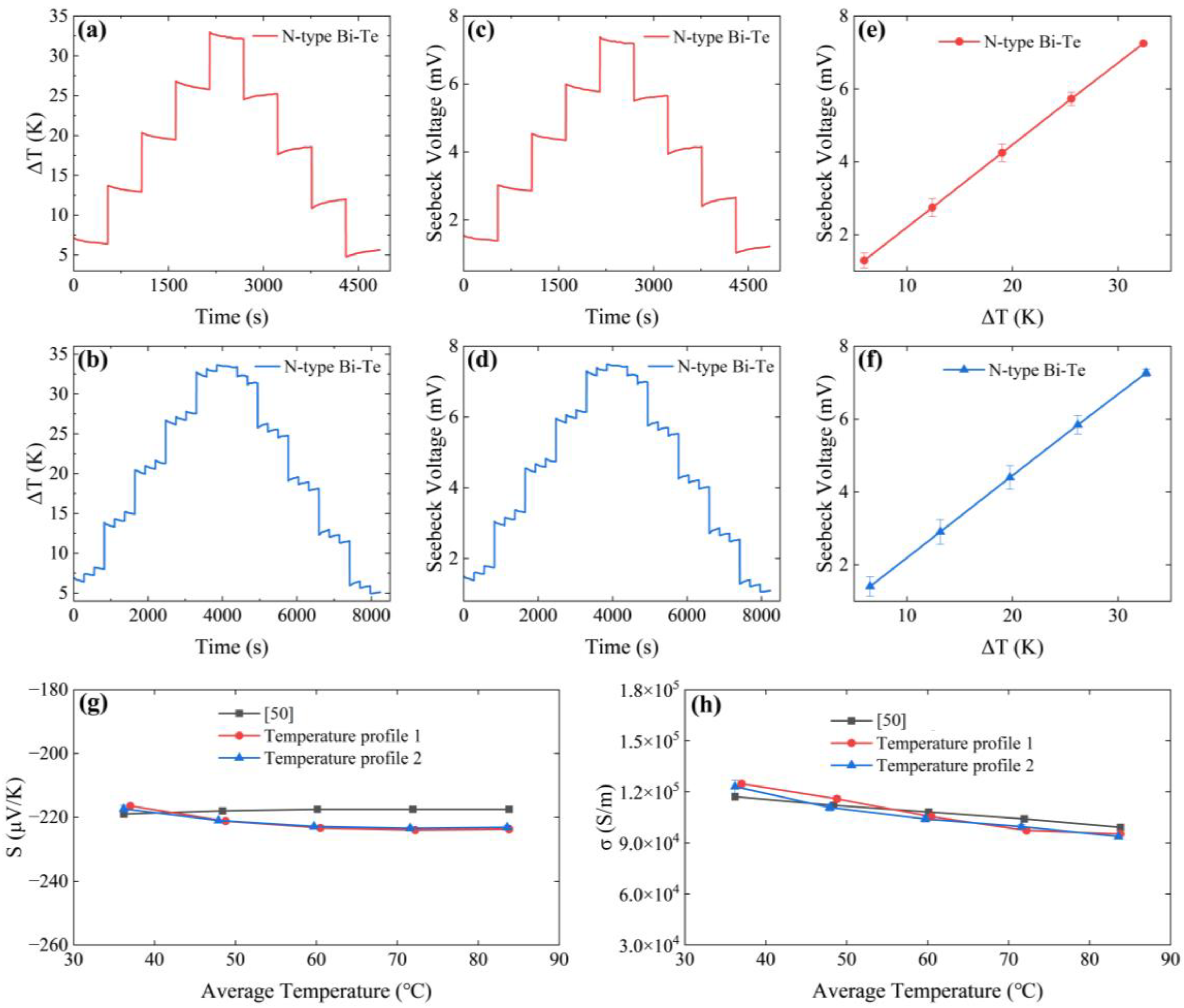
Figure 7 displays a set of experimental results conducted on N-type Bi-Te over a temperature range from room temperature to 100 °C. The average temperatures depicted in Figure 7 are the mean value of the cold-end and hot-end temperatures. The larger size of the N-type sample (12 mm × 12 mm × 20 mm) allowed for applying larger temperature gradients and obtaining higher Seebeck voltages. It is because in a longer specimen, heat flux faces a larger thermal resistance as it needs to flow through an extended path. When one end of the specimen is heated, the heat takes longer to diffuse across the entire length, enabling a larger temperature differential (∆T) across the length of the sample. The maximum average temperature difference of 32.4 K in Figure 7a,b corresponds to the maximum average Seebeck voltage of 7.9 mV in Figure 7c,d. The nearly identical SVs in Figure 7c,d generated by different temperature profiles in Figure 7a,b indicate the reproducibility of the experimental measurements, highlighting the accuracy and reliability of the constructed apparatus. Figure 7g,h demonstrate good agreement between the measured S and σ values of the samples obtained using the devised testing system and the reference values provided by the ingot manufacturing company. The difference in the S and σ values of the samples is estimated to be within 3% and 6.6%, respectively, further validating the accuracy of the measurement system.

4. Conclusions

This article presents the design, fabrication, and evaluation of a specialized apparatus developed for the simultaneous measurement of the Seebeck coefficient and electrical resistivity. The study provides an in-depth exploration of the apparatus’s architectural design and the data processing approach adopted. The integration of LabVIEW seamlessly manages commercially available electronic instruments, enhancing the measurement process. The apparatus excels in accurately controlling the temperature gradient between the cold and hot ends of the sample, covering temperatures from room temperature to 100 °C, with an excellent precision of ±0.05 °C. The LabVIEW programming efficiently manages multiple tasks, including data acquisition, presentation, processing, and storage. These tasks involve resistance, resistivity, Seebeck voltage, and Seebeck coefficient measurements during the sample characterization at various temperature stages. Furthermore, the developed Graphical User Interfaces present real-time temperature profiles, circuit voltage, and current signals, as well as the analysis results. These interfaces serve to exhibit real-time voltage and current signals as well. By analyzing current-voltage (I–V) characteristics, the method enables simultaneous determination of the Seebeck voltage and resistance of the sample. This systematic approach involves evaluating the material’s response across different current or voltage settings. Employing mathematical models and curve-fitting techniques, the method accurately extracts Seebeck voltage and internal resistance from the resulting I–V curves, effectively mitigating errors stemming from contact resistance. Furthermore, the adoption of an AC four-point probe methodology serves to minimize the potential impact of Joule heating-induced thermoelectric potential during resistance measurements. This versatile apparatus is particularly suited for assessing the electrical properties of conventional thermoelectric materials, such as degenerate semiconductors featuring low resistance and high Seebeck coefficients. Experimental findings indicate the robustness of the measurements, displaying a data consistency of less than 10% when compared to results obtained using commercial systems.

References

- Bell, L.E. Cooling, Heating, Generating Power, and Recovering Waste Heat with Thermoelectric Systems. Science 2008, 321, 1457–1461. [Google Scholar] [CrossRef]
- Shi, X.; Zou, J.; Chen, Z. Advanced Thermoelectric Design: From Materials and Structures to Devices. Chem. Rev. 2020, 120, 7399–7515. [Google Scholar] [CrossRef]
- Wei, J.; Yang, L.; Ma, Z.; Song, P.; Zhang, M.; Ma, J.; Yang, F.; Wang, X. Review of current high-ZT thermoelectric materials. J. Mater. Sci. 2020, 55, 12642–12704. [Google Scholar] [CrossRef]
- Zhou, Z.; Uher, C. Apparatus for Seebeck coefficient and electrical resistivity measurements of bulk thermoelectric materials at high temperature. Rev. Sci. Instrum. 2005, 76, 023901. [Google Scholar] [CrossRef]
- Wood, C.; Chmielewski, A.; Zoltan, D. Measurement of Seebeck coefficient using a large thermal gradient. Rev. Sci. Instrum. 1988, 59, 951–954. [Google Scholar] [CrossRef]
- Martin, J. Apparatus for the high temperature measurement of the Seebeck coefficient in thermoelectric materials. Rev. Sci. Instrum. 2012, 83, 065101. [Google Scholar] [CrossRef]
- Martin, J.; Wong-Ng, W.; Green, M.L. Seebeck Coefficient Metrology: Do Contemporary Protocols Measure Up? J. Electron. Mater. 2015, 44, 1998–2006. [Google Scholar] [CrossRef]
- Wang, C.; Chen, F.; Sun, K.; Chen, R.; Li, M.; Zhou, X.; Sun, Y.; Chen, D.; Wang, G. Contributed Review: Instruments for measuring Seebeck coefficient of thin film thermoelectric materials: A mini-review. Rev. Sci. Instrum. 2018, 89, 101501. [Google Scholar] [CrossRef]
- Sharma, S.; Yadav, C.S. Experimental setup for the Seebeck and Nernst coefficient measurements. Rev. Sci. Instrum. 2020, 91, 123907. [Google Scholar] [CrossRef]
- Ferreira-Teixeira, S.; Carpinteiro, F.; Araújo, J.P.; Sousa, J.B.; Pereira, A.M. Versatile Seebeck and electrical resistivity measurement setup for thin films. Rev. Sci. Instrum. 2021, 92, 043904. [Google Scholar] [CrossRef]
- Ponnambalam, V.; Lindsey, S.; Hickman, N.S.; Tritt, T.M. Sample probe to measure resistivity and thermopower in the temperature range of 300–1000K. Rev. Sci. Instrum. 2006, 77, 073904. [Google Scholar] [CrossRef]
- Martin, J.; Nolas, G.S. Apparatus for the measurement of electrical resistivity, Seebeck coefficient, and thermal conductivity of thermoelectric materials between 300 K and 12 K. Rev. Sci. Instrum. 2016, 87, 015105. [Google Scholar] [CrossRef]
- Haupt, S.; Edler, F.; Bartel, M.; Pernau, H.F. Van der Pauw device used to investigate the thermoelectric power factor. Rev. Sci. Instrum. 2020, 91, 115102. [Google Scholar] [CrossRef]
- Dörling, B.; Zapata-Arteaga, O.; Campoy-Quiles, M. A setup to measure the Seebeck coefficient and electrical conductivity of anisotropic thin-films on a single sample. Rev. Sci. Instrum. 2020, 91, 105111. [Google Scholar] [CrossRef] [PubMed]
- Yang, X.; Wang, C.; Lu, R.; Shen, Y.; Zhao, H.; Li, J.; Li, R.; Zhang, L.; Chen, H.; Zhang, T.; et al. Progress in measurement of thermoelectric properties of micro/nano thermoelectric materials: A critical review. Nano Energy 2022, 101, 107553. [Google Scholar] [CrossRef]
- Patel, A.; Pandey, S.K. Automated instrumentation for the determination of the high-temperature thermoelectric figure-of-merit. Instrum. Sci. Technol. 2018, 46, 600–613. [Google Scholar] [CrossRef]
- Patel, A.; Pandey, S.K. Automated instrumentation for high-temperature Seebeck coefficient measurements. Instrum. Sci. Technol. 2017, 45, 366–381. [Google Scholar] [CrossRef]
- Yadam, S.; Dev, A.; Das, R.; Rao Hari, S.; Ramachandra Rao, M.S.; Sankaranarayanan, V.; Sethupathi, K. Design and fabrication of thermopower and electrical resistivity setup for bulk and thin film systems. Cryogenics 2022, 127, 103550. [Google Scholar] [CrossRef]
- Wang, H.; Yang, F.; Guo, Y.; Peng, K.; Wang, D.; Chu, W.; Zheng, S. Determination of the thermopower of microscale samples with an AC method. Measurement 2019, 131, 204–210. [Google Scholar] [CrossRef]
- Masoumi, S.; Noori, A.; Shokrani, M.; Hossein-Babaei, F. Apparatus for Seebeck Coefficient Measurements on High-Resistance Bulk and Thin-film Samples. IEEE Trans. Instrum. Meas. 2020, 69, 3070–3077. [Google Scholar] [CrossRef]
- Iwanaga, S.; Toberer, E.S.; LaLonde, A.; Snyder, G.J. A high temperature apparatus for measurement of the Seebeck coefficient. Rev. Sci. Instrum. 2011, 82, 063905. [Google Scholar] [CrossRef]
- Martin, J.; Tritt, T.; Uher, C. High temperature Seebeck coefficient metrology. J. Appl. Phys. 2010, 108, 121101. [Google Scholar] [CrossRef]
- Mackey, J.; Dynys, F.; Sehirlioglu, A. Uncertainty analysis for common Seebeck and electrical resistivity measurement systems. Rev. Sci. Instrum. 2014, 85, 085119. [Google Scholar] [CrossRef]
- Guan, A.; Wang, H.; Jin, H.; Chu, W.; Guo, Y.; Lu, G. An experimental apparatus for simultaneously measuring Seebeck coefficient and electrical resistivity from 100 K to 600 K. Rev. Sci. Instrum. 2013, 84, 043903. [Google Scholar] [CrossRef]
- Rouleau, O.; Alleno, E. Measurement system of the Seebeck coefficient or of the electrical resistivity at high temperature. Rev. Sci. Instrum. 2013, 84, 105103. [Google Scholar] [CrossRef]
- Fu, Q.; Xiong, Y.; Zhang, W.; Xu, D. A setup for measuring the Seebeck coefficient and the electrical resistivity of bulk thermoelectric materials. Rev. Sci. Instrum. 2017, 88, 095111. [Google Scholar] [CrossRef]
- Böttger, P.H.M.; Flage-Larsen, E.; Karlsen, O.B.; Finstad, T.G. High temperature Seebeck coefficient and resistance measurement system for thermoelectric materials in the thin disk geometry. Rev. Sci. Instrum. 2012, 83, 025101. [Google Scholar] [CrossRef]
- He, X.; Yang, J.; Jiang, Q.; Luo, Y.; Zhang, D.; Zhou, Z.; Ren, Y.; Li, X.; Xin, J.; Hou, J. A new method for simultaneous measurement of Seebeck coefficient and resistivity. Rev. Sci. Instrum. 2016, 87, 124901. [Google Scholar] [CrossRef]
- Beretta, D.; Bruno, P.; Lanzani, G.; Caironi, M. Reliable measurement of the Seebeck coefficient of organic and inorganic materials between 260 K and 460 K. Rev. Sci. Instrum. 2015, 86, 075104. [Google Scholar] [CrossRef]
- Mulla, R.; Glover, K.; Dunnill, C.W. An Easily Constructed and Inexpensive Tool to Evaluate the Seebeck Coefficient. IEEE Trans. Instrum. Meas. 2021, 70, 3021512. [Google Scholar] [CrossRef]
- Jaafar, W.M.N.W.; Snyder, J.E.; Min, G. Apparatus for measuring Seebeck coefficient and electrical resistivity of small dimension samples using infrared microscope as temperature sensor. Rev. Sci. Instrum. 2013, 84, 054903. [Google Scholar] [CrossRef] [PubMed]
- Sharma, P.K.; Sharma, V.K.; Senguttuvan, T.D.; Chaudhary, S. Design, fabrication and calibration of low cost thermopower measurement set up in low- to mid-temperature range. Measurement 2020, 150, 107054. [Google Scholar] [CrossRef]
- Cervantes, A.d.J.R.; Gonzalez, E.R.; Alvarez, J.C. Development and Automation of a Thermoelectric Characterization System. In Proceedings of the 2018 International Conference on Mechatronics, Electronics and Automotive Engineering (ICMEAE), Cuernavaca, Mexico, 26–29 November 2018; pp. 98–101. [Google Scholar]
- Tripathi, T.S.; Karppinen, M. Experimental setup for anisotropic thermoelectric transport measurements using MPMS. Meas. Sci. Technol. 2019, 30, 025602. [Google Scholar] [CrossRef]
- Ider, J.; Oliveira, A.; Rubinger, R.M. A Robust System for Thermoelectric Device Characterization. IEEE Trans. Instrum. Meas. 2021, 70, 3115213. [Google Scholar] [CrossRef]
- Yoshino, T.; Wang, R.; Gomi, H.; Mori, Y. Measurement of the Seebeck coefficient under high pressure by dual heating. Rev. Sci. Instrum. 2020, 91, 035115. [Google Scholar] [CrossRef]
- Min, G. Principle of determining thermoelectric properties based on I–V curves. Meas. Sci. Technol. 2014, 25, 085009. [Google Scholar] [CrossRef]
- Borup, K.A.; De Boor, J.; Wang, H.; Drymiotis, F.; Gascoin, F.; Shi, X.; Chen, L.; Fedorov, M.I.; Müller, E.; Iversen, B.B. Measuring thermoelectric transport properties of materials. Energy Environ. Sci. 2015, 8, 423–435. [Google Scholar] [CrossRef]
- Seebeck Coefficient/Electric Resistance Measurement System ZEM-3 Series. Available online: https://advance-riko.com/en/products/zem-3/ (accessed on 4 July 2023).
- LSR-3 Seebeck-Coefficient/Resistivity System. Available online: https://www.linseis.com/en/products/thermoelektric/lsr-3/ (accessed on 4 July 2023).
- Seebsys—Combined Seebeck Coefficient and Resistance Measurement System Description. Available online: https://www.norecs.com/index.php?page=Home (accessed on 4 July 2023).
- Physical Property Measurement System (PPMS). Available online: https://qd-europe.com/be/en/product/physical-property-measurement-system-ppms/ (accessed on 4 July 2023).
- Wei, T.R.; Guan, M.; Yu, J.; Zhu, T.; Chen, L.; Shi, X. How to Measure Thermoelectric Properties Reliably. Joule 2018, 2, 2183–2188. [Google Scholar] [CrossRef]
- Lowhorn, N.D.; Wong-Ng, W.; Lu, Z.Q.; Martin, J.; Green, M.L.; Bonevich, J.E.; Thomas, E.L.; Dilley, N.R.; Sharp, J. Development of a Seebeck coefficient Standard Reference Material™. J. Mater. Res. 2011, 26, 1983–1992. [Google Scholar] [CrossRef]
- Mackey, J.; Sehirlioglu, A.; Dynys, F. Detailed Uncertainty Analysis of the ZEM-3 Measurement System. In Proceedings of the International Conference on Thermoelectrics, Nashville, TN, USA, 6–10 July 2014. [Google Scholar]
- Mackey, J.; Sehirlioglu, A.; Dynys, F. Uncertainty analysis of Seebeck coefficient and electrical resistivity characterization. In Proceedings of the Electronic Materials and Applications, Orlando, FL, USA, 22–24 January 2014. [Google Scholar]
- Liu, Y.; Fu, C.; Xie, H.; Zhao, X.; Zhu, T. Reliable measurements of the Seebeck coefficient on a commercial system. J. Mater. Res. 2015, 30, 2670–2677. [Google Scholar] [CrossRef]
- Lowhorn, N.D.; Wong-Ng, W.; Lu, Z.Q.; Thomas, E.; Otani, M.; Green, M.; Dilley, N.; Sharp, J.; Tran, T.N. Development of a Seebeck coefficient Standard Reference Material. Appl. Phys. A Mater. 2009, 96, 511–514. [Google Scholar] [CrossRef]
- Sebek, J.; Santava, E. Influence of the sample mounting on thermal conductance measurements using PPMS TTO option. J. Phys. Conf. Ser. 2009, 150, 012044. [Google Scholar] [CrossRef]
- Commercial Bi2Te3-Based Thermoelectric Ingot. Available online: http://www.thermonamic.com.cn/pro_view.asp?id=795 (accessed on 4 July 2023).
Figure 1.
Block diagram of the apparatus used for measuring the Seebeck coefficient and resistivity.
Figure 2.
Schematics and photograph of the measurement system. (a) Three-dimensional overview of the sample holder. (b) Close-up view of the sample. (c) Photo of the sample holder. (d) Photograph of the measurement apparatus.
Figure 3.
(a) Schematic diagram showing the principle of resistance and Seebeck voltage measurements. (b) Equivalent circuit, consisting of a thermoelectric potential and an internal resistance. (c) I–V curves of a thermoelectric sample under a constant ΔT.
Figure 4.
Schematic block diagram of the measurement system.
Figure 5.
LabVIEW algorithm for measurement in the devised apparatus.
Figure 6.
(a,b) Temporal temperature profiles 1 and 2 of the applied temperature difference (ΔT) between the cold and hot ends of a P-type Bi-Te sample. (c,d) The corresponding generated Seebeck voltage (SV) of temperature profiles 1 and 2. (e,f) Plot of SV versus ΔT for temperature profiles 1 and 2. (g,h) Comparison of the measured Seebeck coefficient (S) and electrical conductivity (σ) over a temperature range.
Figure 7.
(a,b) Temporal temperature profiles 1 and 2 of the applied temperature difference (ΔT) between the cold and hot ends of an N-type Bi-Te sample. (c,d) The corresponding generated Seebeck voltage (SV) of temperature profiles 1 and 2. (e,f) Plot of SV versus ΔT for temperature profiles 1 and 2. (g,h) Comparison of the measured Seebeck coefficient (S) and electrical conductivity (σ) over a temperature range.
Disclaimer/Publisher’s Note: The statements, opinions and data contained in all publications are solely those of the individual author(s) and contributor(s) and not of MDPI and/or the editor(s). MDPI and/or the editor(s) disclaim responsibility for any injury to people or property resulting from any ideas, methods, instructions or products referred to in the content. |
© 2023 by the authors. Licensee MDPI, Basel, Switzerland. This article is an open access article distributed under the terms and conditions of the Creative Commons Attribution (CC BY) license (https://creativecommons.org/licenses/by/4.0/).
Share and Cite
MDPI and ACS Style
Xiong, R.; Masoumi, S.; Pakdel, A. An Automatic Apparatus for Simultaneous Measurement of Seebeck Coefficient and Electrical Resistivity. Energies 2023, 16, 6319. https://0-doi-org.brum.beds.ac.uk/10.3390/en16176319
AMA Style
Xiong R, Masoumi S, Pakdel A. An Automatic Apparatus for Simultaneous Measurement of Seebeck Coefficient and Electrical Resistivity. Energies. 2023; 16(17):6319. https://0-doi-org.brum.beds.ac.uk/10.3390/en16176319
Chicago/Turabian StyleXiong, Ruifeng, Saeed Masoumi, and Amir Pakdel. 2023. "An Automatic Apparatus for Simultaneous Measurement of Seebeck Coefficient and Electrical Resistivity" Energies 16, no. 17: 6319. https://0-doi-org.brum.beds.ac.uk/10.3390/en16176319
Note that from the first issue of 2016, this journal uses article numbers instead of page numbers. See further details here.