
Numerical Investigation of Hydrogen Jet Dispersion Below and Around a Car in a Tunnel

Environmental Research Laboratory, INRASTES, National Centre for Scientific Research Demokritos, Patriarchou Grigoriou E & 27 Neapoleos Str., 15341 Agia Paraskevi, Greece
*
Author to whom correspondence should be addressed.
Energies 2023, 16(18), 6483; https://0-doi-org.brum.beds.ac.uk/10.3390/en16186483
Submission received: 28 June 2023
/
Revised: 7 August 2023
/
Accepted: 31 August 2023
/
Published: 8 September 2023
(This article belongs to the Special Issue Computational Fluid Dynamics Applied to Hydrogen Safety)
Abstract
:Accidental release from a hydrogen car tank in a confined space like a tunnel poses safety concerns. This Computational Fluid Dynamics (CFD) study focuses on the first seconds of such a release, which are the most critical. Hydrogen leaks through a Thermal Pressure Relief Device (TPRD), forms a high-speed jet that impinges on the street, spreads horizontally, recirculates under the chassis and fills the area below it in about one second. The “fresh-air entrainment effect” at the back of the car changes the concentrations under the chassis and results in the creation of two “tongues” of hydrogen at the rear corners of the car. Two other tongues are formed near the front sides of the vehicle. In general, after a few seconds, hydrogen starts moving upwards around the car mainly in the form of buoyant blister-like structures. The average hydrogen volume concentrations below the car have a maximum of 71%, which occurs at 2 s. The largest “equivalent stoichiometric flammable gas cloud size Q9” is 20.2 m3 at 2.7 s. Smaller TPRDs result in smaller hydrogen flow rates and smaller buoyant structures that are closer to the car. The investigation of the hydrogen dispersion during the initial stages of the leak and the identification of the physical phenomena that occur can be useful for the design of experiments, for the determination of the TPRD characteristics, for potential safety measures and for understanding the further distribution of the hydrogen cloud in the tunnel.
1. Introduction
Hydrogen is expected to play a major role in the energy sector in the near future. The reasons for this, as well as some perspectives of the hydrogen economy, are summarized in [1]. Information regarding the use of hydrogen as a fuel and energy carrier and the role of hydrogen in the energy transition can be found in [2,3,4,5,6]. The potential extensive use of hydrogen poses safety concerns though, due to its wide flammability limits (volume concentrations of 4–75%) and the fact that it burns very fast, especially at concentrations close to its stoichiometric 29.5 vol%. Fundamental information regarding safety issues relevant to this study are given in “Fundamentals of Hydrogen Safety Engineering” [7,8].
The use of hydrogen in transportation is attractive due to zero emissions, high autonomy and fast refuelling. Even though hydrogen can be burnt directly into internal combustion engines, almost all modern hydrogen vehicles of the last two decades use fuel-cell technology [9], which is more efficient. Key components of fuel-cell (hydrogen) road vehicles and their infrastructure are summarized in [10]. In 2021, there were about 51,600 hydrogen vehicles in the world, compared to over 16.5 million electric cars with batteries [11]. The main reason for the limited deployment of fuel-cell cars is the absence of hydrogen distribution networks. As of November 2022, there were only 810 hydrogen fuelling stations for road vehicles worldwide [12]. However, with the increasing demand for hydrogen use, the relevant infrastructure will probably be developed soon. Innovative hydrogen storage and production techniques [13] could also accelerate hydrogen use in the near future.
In addition to the infrastructure, more regulations and standards should be developed in order to provide the legal framework for extensive hydrogen use. The buoyant nature of hydrogen distinguishes it from traditional fossil fuels. The buoyancy provides a safety advantage in open spaces, but it is a serious concern in confined or semi-confined spaces like road tunnels. In cases in which a substantial amount of hydrogen is released and dispersed in a tunnel, a fire and even an explosion might occur. The European research project HyTunnel-CS dealt with the “Pre-normative research for safety of hydrogen driven vehicles and transport through tunnels and similar confined spaces” in order to provide the basis for the development of relevant regulations. In the current work—which was partly conducted within the HyTunnel project—we focus on the downwards accidental blowdown release and dispersion of hydrogen around a car during the initial stage of the release, which has a more general interest regardless of tunnels. In the case of an accident, the first seconds of hydrogen dispersion close to the vehicle are considered to be the most critical ones because—as will be presented in Section 3—the most dangerous hydrogen cloud appears during the first seconds and the very low ignition energy of hydrogen makes its ignition more probable shortly after the start of the release. The initial dispersion is important even in non-ignition cases because it affects the subsequent cloud propagation.
Numerous computational studies that include hydrogen dispersion around a vehicle exist in the literature. Twenty years ago, Venetsanos et al. [14], using the Computational Fluid Dynamics (CFD) methodology, studied an accident that happened in Stockholm in 1983 after the release of approximately 13.5 kg of hydrogen from pressure vessels on a delivery truck. The simulations predicted a substantial amount of an about 600 m3 hydrogen flammable cloud inside the street canyon at the estimated time of ignition, about 10 s after the start of the release. Later studies that included hydrogen dispersion inside a tunnel [15], in a refuelling station [16], inside a garage [17] and in an underpass [18] revealed the high potential of CFD regarding hydrogen safety studies in confined or semi-confined spaces.
Middha and Hansen [19], using CFD, investigated various scenarios, including car and bus hydrogen accidents in horseshoe tunnels for several longitudinal ventilation speeds. This work contributed to understanding the risk posed by hydrogen vehicles in road tunnels. One of the car cases involved the downwards release of 5 kg of hydrogen from a 4 mm orifice of a 700-bar tank, with a duration of 84 s. For that case, the maximum flammable gas cloud size was 268 m3 and the maximum “equivalent stoichiometric flammable gas cloud size Q9” was 17.75 m3. Other early studies providing the dispersion of hydrogen from cars in tunnels were presented at conferences [20,21]. Houf et al. [22] used CFD to examine the release of a total of 5 kg of hydrogen from three 700-bar tanks in a transversely ventilated tunnel. They provided the flammable cloud isosurface at 2 s after the start of the release, which surrounded the car from almost all sides and expanded a few metres around it. Other relevant CFD studies include the dispersion of a small leak from below a car in a garage [23], the use of portable blowers to reduce the hydrogen concentrations around a car [24,25] and dispersion in subsea tunnels [26].
More recently, Li and Luo [27]—along with the previous work of Li et al. [28]—examined the dispersion around a car in the open atmosphere due to a downwards hydrogen leakage from a Thermally Activated Pressure Relief Device (TPRD) of 4.2 mm. Tank pressures of both 350 and 700 bars were examined, and the geometry of a real car was reproduced. The blowdown process was analysed, and the diminishing mass flow rate of hydrogen with time was calculated, resulting in a total blowdown time of less than 75 s for the 700-bar tank. They pointed out the problem of the “preferential” diffusion directions of the calculations due to the high velocity gradients following the strong jet impingement of hydrogen against the street. They stated that the “delayed” ignition of hydrogen is more dangerous and concluded that the most hazardous timeframe occurs within ten seconds of the initiation of the release. In all cases of dispersion and fire and in any direction, a separation distance of 12 m for the general public is reported to be adequately safe.
Hussein et al. [29] examined various hydrogen release scenarios from cars in a naturally ventilated car park. They considered a 700-bar tank, TPRD sizes between 0.5 mm and 3.34 mm and downward release angles of 0, 30 and 45 degrees. For all spatial discretisations, they used second-order upwind numerical schemes. In the results, they provided concentration isosurfaces around the car of a simplified geometry, from which it can be observed that, in the case of downward release with an angle of 0 degrees, hydrogen surrounds the car at specific points, namely, from the back and from its sides. Isosurfaces were provided for later stages also, showing the dispersion of hydrogen along the ceiling. In all cases, the maximum flammable cloud was formed before the time of 20 s, and it decreased with the decreasing TPRD size. Finally, the oblique release directions were considered favourable because, in those cases, hydrogen did not surround the car. An independent but similar study was performed by Shentsov et al. [30]. They examined releases from TPRDs of 0.5–2 mm and various ventilation strengths and release directions. They concluded that smaller TPRDs result in smaller flammable clouds, and that a downwards release direction of 45 degrees is preferable, as long as it is not directed towards obstacles like walls. The main contribution of these two studies is that smaller TPRDs and oblique release directions should, in general, be considered safer.
Li et al. [31] investigated the dispersion and combustion of an upwards hydrogen release in a horseshoe-shaped tunnel with many vehicles, using the CFD code GASFLOW-MPI. A typical blowdown was considered, with an initial mass flow rate of 0.5 kg/s. Regarding the dispersion, the study concluded that hydrogen accumulates beneath the ceiling, forming a thin layer with strong concentration gradients. The highest volume concentration of the topmost layer was about 40%.
Huang et al. [32] used Large-Eddy Simulation (LES) to study the dispersion around a car in a garage with various ventilation scenarios. They considered a downwards release of 0.003 kg/s and presented the irregular escaping of hydrogen from the back and the sides of the car. Hansen et al. [33] studied upwards and downwards TPRD releases from hydrogen heavy-duty vehicles (HDVs) in tunnels for various tanks and TPRD diameters. They concluded that upwards releases are safer for HDVs.
Lv et al. [34] and Shen et al. [35] examined the hydrogen dispersion in an open garage for various parking scenarios and upwards and downwards releases from a 700-bar tank through TPRDs of diameters between 2 mm and 4 mm. They argued that analysing free unignited hydrogen release is fundamental for studying the possible disastrous consequences of hydrogen leakage, and they provided both the flammable and the equivalent stoichiometric gas Q9 cloud volumes for each TPRD case. They showed that larger TPRD diameters resulted not only in a larger envelope of the flammable gas cloud, but also in a faster dissipation.
In the current work, the dispersion of hydrogen escaping from a downwards-pointing TPRD of a car inside a tunnel is considered. The study focuses on the area around the vehicle, especially at the initial stages of the release, and more specifically on the physical effects that take place during the first seconds. The numerical parameters that may affect the flow and dispersion field are discussed, and many relevant sensitivity tests were performed in order to identify their effect on the reliability and accuracy of the results. The main aim of the study is to attempt to identify and understand the underlying physical phenomena of the hydrogen dispersion below and around the car and assess how they affect the further propagation of the cloud inside the tunnel. In order to better understand the effect of the physical parameters, several tests were performed examining parameters like the source mass flow rate, the distance of the car from the street, the under-chassis geometry (with and without wheels) and even the existence of the car itself. This work is of general interest and most of its conclusions can be exploited regardless of the existence of a tunnel.
The rest of this paper is structured as follows: Section 2 introduces the problem examined and the solution methodology, including the treatment of the source. The main part of Section 3 is its first subsection, namely Section 3.1, which presents in detail the hydrogen jet dispersion below and around the car and includes the description of the main physical phenomena observed, which are the focus of this paper. The other two subsections of Section 3 are supplementary and mainly investigate how general the phenomena discussed in Section 3.1 are. More specifically, in Section 3.2, different but similar physical problems are examined, as, for example, the case of the greater distance of the car from the street. In Section 3.3, the effect of different key numerical choices is studied—including the discretisation scheme—and some relevant guidelines are provided. In Section 4, the first paragraph presents the main conclusions of the study and relates to Section 3.1. The second and third paragraphs summarise Section 3.2 and Section 3.3 and include best-practice guidelines. The final paragraph of the conclusions provides future perspectives.
2. Methodology
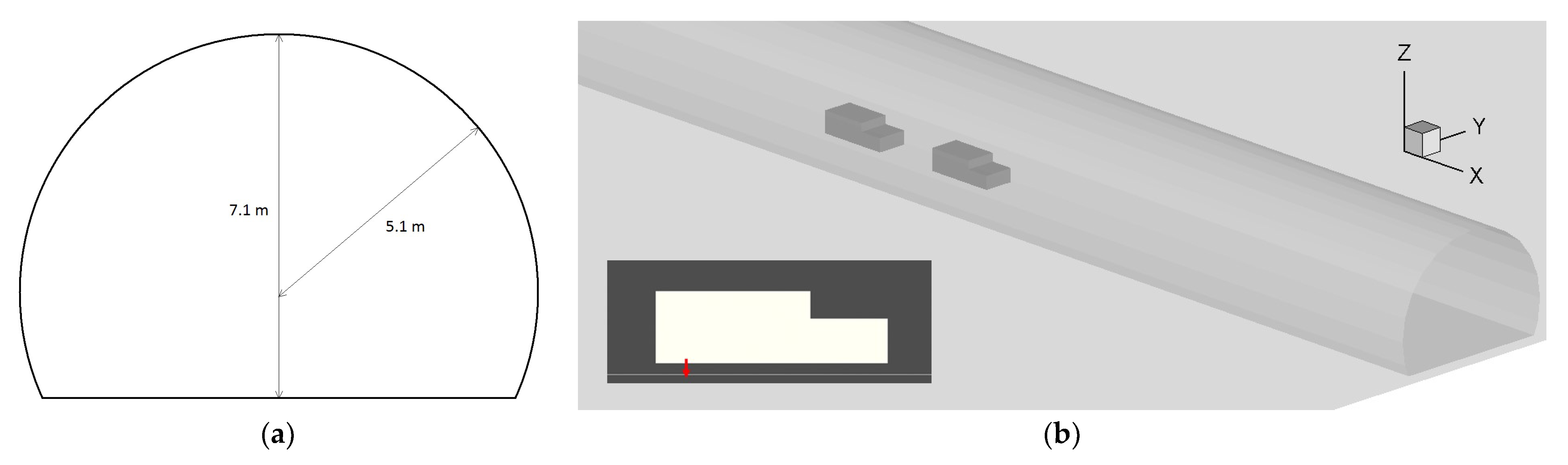
The physical problem considered involves an accidental release of hydrogen from a fuel-cell car in a non-ventilated tunnel. Six kilograms of hydrogen leak through a TPRD from a 700-bar tank. A typical horseshoe-shaped tunnel is assumed with a cross section of 60.72 m2 and a total height of 7.1 m (Figure 1). In the “base case”, an 80 m long part of the tunnel is examined with two simple cars with dimensions of 4.2 m × 1.8 m × 1.3 m placed at the tunnel centreline. Concerning the coordinate system used, the zero point of the Z axis is at the centre of the tunnel circle, and the street is at the Z = −2 m level. The release is downwards and is located at distances of 0.5 m from the back of the first car and 0.2 m from the ground (inset of Figure 1b). The release point is at the middle of the tunnel and its coordinates are (0, 0, −1.8).
The simulations were performed using the ADREA-HF CFD code, which has been extensively validated in the past for hydrogen dispersion applications, including cases of confined and semi-confined geometries [36,37,38,39,40]. The Unsteady Reynolds-Averaged Navier–Stokes (URANS) methodology was used with the finite-volume method on a staggered Cartesian grid. Complex geometries are handled with the use of porosities [41]. The basic governing equations are presented below, while more information about the code and its mathematical formulation can be found in [36,42,43].
The Favre-averaged Navier–Stokes equations with the Boussinesq assumption for the Reynolds stresses are solved, along with the equation for the hydrogen mass fraction (Einstein summation notation is used):
where ρ is the density; t is the time; ui are the velocity components (i = 1, 2, 3); xi are the spatial coordinates; p is the pressure; μ is the dynamic viscosity; μt is the turbulent viscosity; gi are the gravitational acceleration components; q is the hydrogen mass fraction; D is the molecular diffusivity of hydrogen to air; Sct is the turbulent Schmidt number, taken as equal to 0.72. The bar represents the time-averaged values, while the tilde denotes the density-weighted time-averaged values. The standard k-ε model [44] is used to estimate the turbulent viscosity:
where k is the turbulent kinetic energy, and ε the dissipation of the turbulent kinetic energy. P and G represent the generation of turbulent kinetic energy due to the velocity gradient and buoyancy, respectively, while Prt is the turbulent Prandl number, taken as equal to 0.72. The following constant values are used: Cμ = 0.09; Cε1 = 1.44; Cε2 = 1.92; σk = 1; σε = 1.3; and Cε3 = 0 if G ≤ 0 or Cε3 = 1 if G > 0.
For the current study, only the dispersion was studied, and no fire was assumed. The flow was considered to be isothermal (20 °C), and thus no energy equation was solved. This is compatible with the Birch notional nozzle approach [45] that was used for the source. The standard k-ε turbulence model was chosen for the base case, as it is the one used in the RANS validation studies of ADREA-HF that have to do with hydrogen dispersion and is the most widely spread [46], something that allows for comparisons with other studies. The initial value of k was 0.0025 m2/s2 in the whole computational domain, while the initial values of ε varied from approximately 0.0004 m2/s3 near walls to 0.00001 m2/s3 along the centreline. Standard rough-type wall functions were considered for all solid objects, with a roughness length of 0.001 m.
In the base case, only an 80 m long part of the tunnel was modelled, and the domain dimensions were 80 × 10.2 × 7.1 m3. At the longitudinal ends of the domain, the zero-gradient boundary condition was used for the v and w velocity components, while constant pressure was used for the u velocity. For the mass fraction of hydrogen, a more complex boundary condition was used: a zero gradient for the case of outflow and a given value (i.e., zero) with no diffusion in the case of inflow. An “extended-domain base case” was also examined. In this case, the whole 200 m tunnel length was considered, and the domain was extended outside of the tunnel in all directions, reaching 260 × 40 × 42 m3. In the small domain, the simulations were usually stopped at 30 s, which is roughly the time that hydrogen reached the small-domain boundaries, while the simulations of the extended domain were stopped at 3000 s, after all the hydrogen escaped from the tunnel. For both domains till the time of 30 s, the results are practically the same. Thus, for the purposes of this work, which focused on the area around the car, the small domain was considered adequate, and most of the sensitivity and parametric studies were performed with this domain.
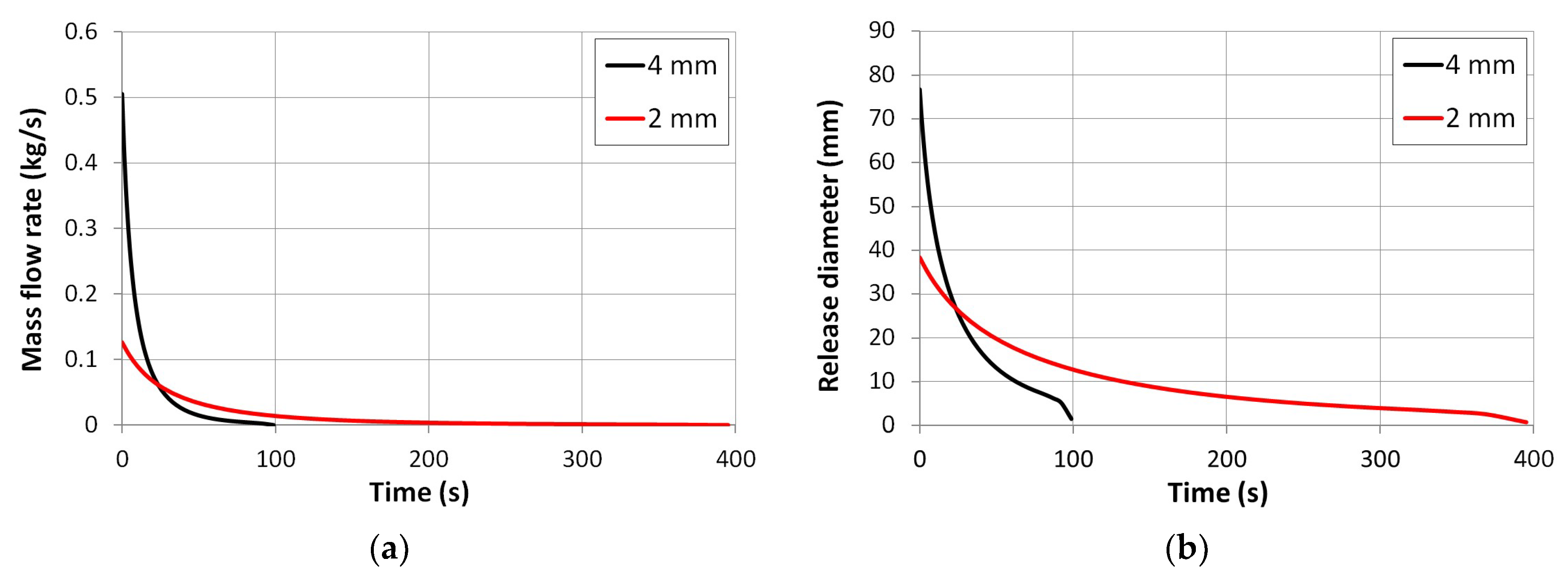
Concerning the source, in the base case, hydrogen is supposed to escape from a TPRD of 4 mm. A TPRD of 2 mm was also tested. The notional nozzle approach was used following the best-practise guidelines [47] in order to avoid the demanding simulation of the complex shock structure near the release point due to the underexpanded jet that is formed. The Birch approach [45] combined with the NIST (National Institute of Standards and Technology) equation of state was used. The source mass flow rate with time was calculated with the use of the “DISCHA” tool developed from the Environmental Research Laboratory, which is also available in [48]. The initial velocity of the hydrogen jet was sonic, and in the simulations, it virtually decreased with time in order to account for the blowdown. In Figure 2, the mass flow rate and the notional nozzle diameter are presented for the two TPRD cases as a function of time. The total release durations were approximately 100 s and 400 s for the 4 mm and 2 mm cases, respectively. The Reynolds number based on the notional nozzle diameter and the sonic hydrogen speed was about 844,000 at the beginning of the release for the 4 mm TPRD case. It is clarified that, in the base case, the mass flow rate practically dropped with time by applying a reduction in the jet speed. The values of Figure 2b were actually used only for the simulations reported in Section 3.3.3, for which the “emitting” surface reduction method was used (see also Section 3.3.3). In all cases examined in this work, the mass flow rate dropped with time in order to accurately account for the blowdown (Figure 2a), even if the actual grid did not change with time.
The source was modelled as a surface at the bottom of the chassis with the appropriate inlet transient boundary conditions in order to release the actual hydrogen mass with time. Due to the small size of the notional diameter, the computational grid (Figure 3) is finer in that region. The source was discretised with four cells to provide a good balance between the accuracy and the computation time. The grid is composed of several sections in order to be aligned with the source and the vehicles. It is uniform in all axes around the source and then expands with ratios between 1.04 and 1.06 in the horizontal directions. In the vertical direction, there are six equidistant cells beneath the car, and the expansion ratios used at the other sections range between 1.06 and 1.1. The total number of cells for the base case is 171 × 84 × 50. Several grid sensitivity tests were performed and are discussed in Section 3.3.2.
The boundary conditions of the source area are “given value and no diffusion” for all variables except k and ε. The velocity components u and v are zero, the initial w equals −1303.5 m/s and the hydrogen mass fraction is one. The total hydrogen mass that enters the domain reduces with time in order to have a flow rate according to Figure 2a. Based on previous experience [49], a zero-gradient boundary condition was chosen for k and ε so as not to suppress the turbulence that should be produced at the boundaries of the source area. In Section 3.3, many of the simulation parameters described here are changed in order to assess their effect.
The choice of the numerical scheme for the convection terms of the discretised equations in the case of an impinging jet plays a critical role, especially in Cartesian grids, like in this work. Tolias and Venetsanos [50] investigated this issue in a previous study and showed that among 15 different convective schemes, the best performance was exhibited by the Fromm [51] and MUSCL [52,53,54] schemes that delivered almost circular horizontal hydrogen propagation.
For the current study, the MUSCL scheme was chosen for the convection terms of all equations. The preference of the MUSCL over the Fromm scheme lays in the fact that the latter is an unbounded scheme, so there were concerns about how physical its results would be away from the impinging area, especially in the presence of obstacles. The use of the Fromm scheme would also result in using a different scheme for the velocities than for the concentrations and the k and ε equations, as, for the latter—which cannot have negative values—we are forced to use the “bounded Fromm” scheme, which is different (and in fact is practically equivalent to the MUSCL scheme). In Section 3.3, more information about the performance of the MUSCL compared with the Fromm scheme is given.
Concerning the convergence criterion, in each iteration, the absolute error (the value in the current iteration minus the value in the previous iteration) is estimated in all cells for each variable. Convergence is achieved when the maximum error is smaller than 0.001 times the maximum value of the variable. For the discretisation of the temporal terms, an implicit scheme is used with first-order backwards differences. The implicit scheme provides the capability of using Courant–Friedrichs–Lewy (CFL) values greater than 1 without having numerical instabilities. In most of the simulations of this work, the maximum CFL number of the whole domain was limited to four. This results in very low time steps, due to the high speeds at the source and the small grid size. The initial time step of around 10−4 s increases slowly due to the blowdown, till it reaches about a ten-times-higher value before the end of the simulation at 30 s. The time-step independency of the results was assured. The total wall-clock simulation time of the base case is about seven days on a modern 4-core personal computer, using the Open-MP (Open multi-processing) parallelisation of the code. Computations were also performed on the “ARIS” Greek supercomputer, using the MPI (Message Passing Interface) parallelisation of the code. ARIS consists of 426 nodes, with two Intel Xeon E5-2680 v2 processors (10 real cores per processor) and 64 GB of RAM per node. The base case needs about three days in 10 cores of one node of ARIS.
3. Results and Discussion
This section is divided into three subsections. In the first one, the results of the base case are presented and discussed. The aim is to understand key features of the flow and concentration fields and try to identify the physical phenomena that take place. In the second subsection, modified cases in terms of problem conditions are presented, such as cases with smaller TPRDs, a different position of the TPRD or a higher distance of the car from the ground, in order to investigate whether our conclusions are valid when the physical parameters of the problem are modified. The third subsection presents sensitivity studies on computational parameters like the choice of the turbulence model, grid or numerical scheme and will help us determine the relevant importance of them.
3.1. Results of the Base Case
3.1.1. First Second of the Release
In Figure 4, the hydrogen concentration contours on the sides of the car (Figure 4, left) and from the top (Figure 4, right) are shown, till the time of 0.05 s after the start of the release.
Figure 4a presents the jet at 0.005 s at the back of the car (grey colour). At the beginning of the release, hydrogen reaches the street at less than 1 ms and starts spreading horizontally. At the same time, the very fast downwards-oriented flow below the source creates a pressure drop. This generates horizontal velocity components just below the chassis towards the source (i.e., in the opposite direction of that of the impingement (street) plane). This, in turn, results in a recirculating flow in the area between the car and the street, as Figure 4a shows. The formation of a recirculation at confined impinging jets is also reported in [58].
In Figure 4b, the plane above the street is presented, at 0.005 s. The contours have an almost circular shape, as in reality, due to the appropriate high-order convective numerical scheme used in the simulations. It is noted that our initially rectangular jet practically behaves as a round jet of the same area. This behaviour is known in the literature [59,60] and, in our case, it is strengthened from the fact that the turbulent kinetic energy of the jet is very high (of the order of 100,000 m2/s2 in the base case).
As the time passes (left column of Figure 4), the horizontal spreading of the impinging hydrogen increases and so does the recirculation size (purple oval in Figure 4a,c,e). The centre of the relevant vortex (purple cross in Figure 4a,c,e) is constantly transferred at higher distances from the jet axis. By the time of 0.02 s (Figure 4e), it has reached the back of the car. Till that time, the hydrogen recirculates between the car and the street and increases the concentrations in this area. After the time of 0.02 s, this behaviour changes at the area of the back of the car, as part of the hydrogen escapes out of the confined space between the car and the street.
At the time of 0.05 s, we can clearly notice that fresh air enters from the back of the car (Figure 4g, red circle) and travels below the chassis towards the source due to the pressure drop mentioned earlier. The entrained air dilutes the hydrogen that is just below the car at the area left of the jet (Figure 4g). Then, it follows the downwards flow of the high-speed jet. This “fresh-air entrainment effect” at the back of the car (Figure 4g, red circle) is a strong physical phenomenon that plays a critical role in the subsequent hydrogen dispersion below the car, for dozens of seconds.
The strong “fresh-air entrainment effect” at the back of the car substantially changes the concentration field below the vehicle. The most obvious and important change (Figure 4g) is the reduction in the concentrations just below the chassis in the area between the jet and the back of the car (cyan in Figure 4g), compared to the rest of the sub-chassis areas (green in Figure 4g).
Figure 4.
The evolution of the impinging jet between 0.005 s and 0.05 s: (a,c,e,g) hydrogen volume fraction (XV_H2) contours at central XZ plane along with the tangential velocity vectors; (b,d,f,h) hydrogen concentration contours at the bottom XY plane of the domain. The contour levels are the same for all the sub-figures.

The “fresh-air entrainment effect” is strong when the recirculation vortex centre of the below-car hydrogen recirculation zone is transferred out of the chassis limits (grey dashed line in Figure 4e), as described above. In our base case, this happens only at the rear part of the car. It is noted that the back of the car is closer to the source, having a distance of 0.5 m from the jet, while the sides of the car have a distance of 0.9 m from the jet. At later times, somewhat similar effects happen at the sides of the car, but their strength is much smaller, and the entrainments are very thin (so we talk about a “weak fresh-air entrainment effect”) because, in this case, the centres of the recirculation vortices remain at the confined area between the street and the car.
In the right column of Figure 4, we see that the circular shape of the hydrogen concentrations is retained for some time. Till 0.02 s (Figure 4f), the symmetry of the impinging jet is practically not influenced by the body of the car. With a closer look though, we can observe—especially in Figure 4h—that the hydrogen spreading is not completely circular. There is a slight tendency of selective propagation in both a “cross” shape and in an “X” shape. This behaviour of the MUSCL numerical scheme at the hydrogen impinging jets can also be observed in [50]. This asymmetric behaviour has a cumulative effect that slightly enhances the hydrogen dispersion in the “X” directions, especially in coarse grids, and this should be taken into account when examining the results.
At later times—after 0.05 s—the presence of the car and the fresh-air entrainment effect have a serious impact on the symmetry of the hydrogen dispersion. In Figure 5, the concentration contours close to the street between 0.1 s and 1 s are presented.
In the left column (Figure 5a,c,e,g), the fresh-air entrainment effect can be clearly identified: on the right of the jet, the concentrations constantly increase below the car and reach above 0.8 after the time of 0.5 s, while on the left—close to the back of the car—they stay at low levels (below 0.1 just under the chassis), due to the entrainment of fresh air.
The jet continues to provide hydrogen that impinges on the street and spreads horizontally. Towards the –X direction, this results in the increase in the hydrogen volume at the propagation front (black circles at Figure 5), where a torus is formed. This is clearer in the case with no car that will be presented in Section 3.2. As the time goes by, the propagation speed decreases—as the spreading fluid has to cover a wider area—and the hydrogen front starts having an upwards-velocity component due to buoyancy.
The horizontal spreading of hydrogen at the other side—towards the front of the emitting car—results in an increase in the concentrations at the street level and finally in the whole area below the car, due to the recirculation vortex of that side. The size of this vortex though does not increase much after the time of 0.2 s, reaching a length of about 1.6 m at the time of 1 s. At the end of the recirculation, there is a hydrogen impingement at the bottom of the car (the point of the particular impingement is marked with a small orange circle in Figure 5a,c,e,g), which results in the further spreading of hydrogen along the chassis towards the front of the car. By the time of 1 s, the hydrogen has almost reached the front end of the car.
The top view of the contours reveals that at t = 0.1 s (Figure 5b) and 0.2 s (Figure 5d), some asymmetries start to form, especially at the back end of the car. These ear-like asymmetries are connected to the fresh-air entrainment effect: as the clean air enters the area below the chassis from the back of the car, it washes away any hydrogen. This phenomenon results in the two “ears” seen, for example, in Figure 5d (red circle). These “ears” or “tongues” are created at the back corners of the car, at the limits of the area of the domination of the fresh-air entrainment. This will be made clearer with the examination of the isosurfaces later on, where we will see that the “ears” in Figure 5 correspond to blister-like structures that are created due to the accumulation of hydrogen there.
In Figure 5f,h, we can see that the red high-concentration area at the right of the jet increases due to the accumulation of hydrogen below the chassis, as described earlier. Part of the hydrogen that is accumulated will escape from the sides of the chassis shortly afterwards. The point at the right of the jet from where a substantial amount of hydrogen first escapes from the area below the car is important because this will affect its subsequent dispersion around the car and ultimately in the tunnel. Where this point will be depends on many parameters, but the fresh-air entrainment effect plays an important role regarding this issue too.
Figure 5.
The evolution of the impinging jet between 0.1 s and 1 s: (a,c,e,g) hydrogen volume fraction (XV_H2) contours at Y = 0 plane (X = 0 plane in the insets) along with the tangential velocity vectors; (b,d,f,h) hydrogen concentration contours at the bottom XY plane of the domain. The contour levels are the same for all the sub-figures and the same as Figure 4.

By the time of 0.1 s (Figure 5b), the below-car recirculations have reached the end of the sides of the chassis. Thus, at the sides, some of the hydrogen is not recirculated below the car and is transferred outside of the confined area between the car and the street (inset of Figure 5c). In such cases, it is possible that small amounts of fresh air (small red circle in the inset of Figure 5c) enter above the recirculation (small purple oval at the inset of Figure 5c) towards the underpressure area of the jet. The small yellow area close to the source that is between the higher-concentration red areas (yellow circle in Figure 5e) is partly due to the small air entrainment from the sides of the vehicle. We can notice from the front and side views of the car in Figure 5c,e,g, that the side air entrainment is much weaker than the air entrainment from the back of the car.
The strong fresh-air entrainment from the back of the car with the aid of the weak fresh-air entrainment from its sides plays an important role in the triangular shape of the high-concentration hydrogen below the car (red areas of Figure 5f,h). As a result of these physical mechanisms, the earlier-mentioned point at which hydrogen first escapes from below the car settles towards the front sides of the vehicle, where two more “ears” are formed (brown circle in Figure 5f; see also streamline “st2” of Figure 6 in the next subsection). We can see that, at the same point, the red area of high concentration becomes wider and behaves as a hydrogen provider. It is noted that, till this time, there is no effect of the existence of the tunnel. The flow-field development and the phenomena mentioned may appear in any hydrogen car with a downwards release of a similar flow rate.
3.1.2. First Thirty Seconds of the Release
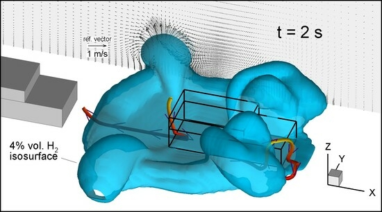
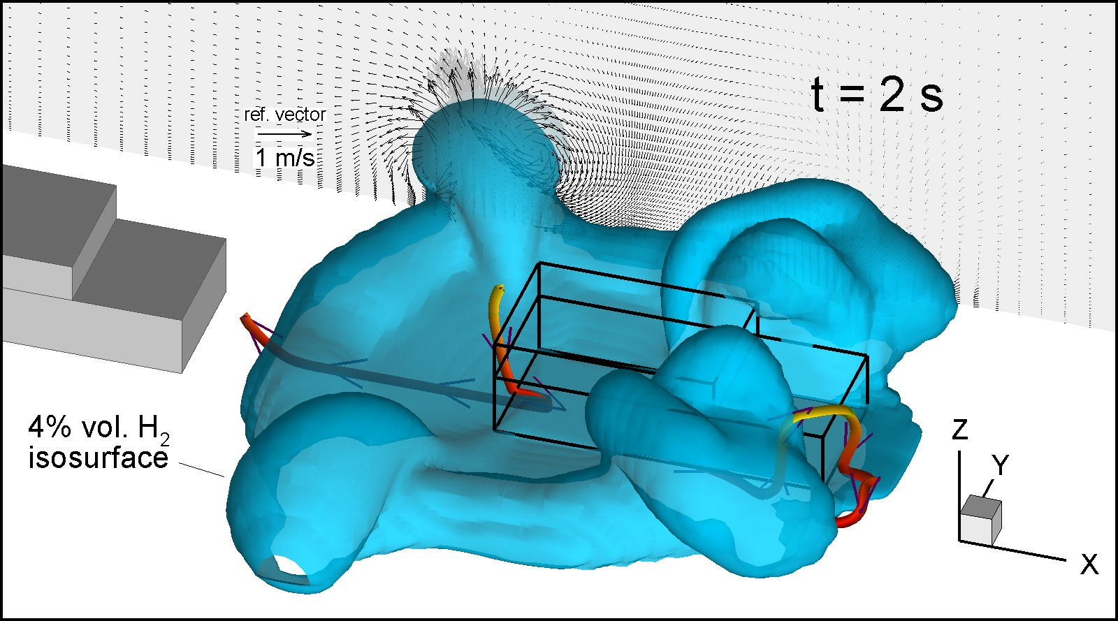
The evolution of the flow field at the time of 2 s (Figure 6a) is directly related to that at the time of 1 s (Figure 5g). The contour levels of Figure 6 are different than those of Figure 5. At the time of 2 s, the street-level hydrogen at the back of the car has propagated further and the torus is bigger, mainly regarding its height. At the other side of the jet, high-concentration hydrogen has reached the front of the car and escapes horizontally from there, due to its momentum. Close to the front edge of the car, the hydrogen starts gathering at the top of the car–street gap, due to its buoyancy (inset of Figure 6a).
In Figure 6b, the 0.2 (green) and the 0.04 (blue, at the inset) volume concentration isosurfaces can be seen. The main and important comment here is the presence of four buoyant blister-like structures that are directly related to the “ears” or “tongues” identified with the red and brown circles in Figure 5. As described in Section 3.1.1, the back blisters are created due to the strong fresh-air entrainment effect from the back of the car that sweeps hydrogen towards them, while the front blisters at the sides of the car are created where hydrogen first escapes from under the chassis.
An important feature of the blister-like structures in Figure 6b is that once they are created, they have the tendency to increase in size. There are two reasons for this. The first one is that because the mechanism of the creation of the blisters is still active, it provides them with more hydrogen. The second reason is that due to the accumulated hydrogen, the buoyancy gives the blisters an upwards-velocity component that drives any underneath hydrogen inside them, which makes them bigger and so on. Thus, these structures—whatever form they take later on—are the main mechanisms that transfer hydrogen upwards, towards the ceiling (crown) of the tunnel. Similar blister-like structures can be noticed in many studies [22,27,28,29,30,34]. The accurate shape and position of these structures depend on many physical and simulation parameters, and the particular shapes should be considered as indicative.
In Figure 6b, between the source and the back blisters, we can see that the isosurfaces form a big-angle “V” shape (faint dashed line in Figure 6b). This “V” is characteristic of the existence of the strong air entrainment effect and marks its dominant area below the car. The “V” is actually a “step” between the low-concentration area that is influenced by the fresh-air entrainment effect (left side of the jet in Figure 6b, close to the back of the car) and the high-concentration area where the jet recirculations dominate below the car and there is no fresh air.
The back blisters start forming their identities after the time of 0.1 s and are initially formed at the corners of the car (Figure 5d) before being transferred (as can be seen from the green isosurface in Figure 6b) from the strong street-level hydrogen flow that is created from the impingement. In the inset of Figure 6b, we can see that the four blister-like structures are connected with a torus—this torus would be the only structure if the car was absent. The interaction of the torus with the front blisters that happens at about t = 1 s (not shown here) creates the complex shape of the front blisters that can be seen in Figure 6b.
Figure 6.
The evolution of the dispersion between 2 s and 20 s: (a,c,e,g) Hydrogen volume fraction (XV_H2) contours at central XZ plane along with the tangential velocity vectors; (b,d,f,h) Hydrogen volume fraction isosurfaces of 0.2 (green) and 0.04 (blue—at the inset).
Figure 6.
The evolution of the dispersion between 2 s and 20 s: (a,c,e,g) Hydrogen volume fraction (XV_H2) contours at central XZ plane along with the tangential velocity vectors; (b,d,f,h) Hydrogen volume fraction isosurfaces of 0.2 (green) and 0.04 (blue—at the inset).

At 5 s, the hydrogen that escapes from the front of the car is immediately transferred upwards, forming a small hydrogen cloud (Figure 6c). Below the chassis there, hydrogen has accumulated towards the top of the car–street gap, leaving space below for fresh air to enter. The velocity vectors near the street at the front of the car point towards the source, forming a small street-level backflow.
Above the front part of the whole car, we can see a big cloudy structure, like a patch. In order to explain its existence, we have to look at the inset of Figure 6d. The front blisters have been transformed to multi-blisters of high complexity, are transferred upwards and have merged where the patch of Figure 6c exists. The back blisters change in shape, increase in size and are transferred upwards, reaching the sides of the tunnel. We see that hydrogen moves towards the ceiling (crown) of the tunnel through the sides of the car at the front and through the sides of the tunnel at the back. The front structures are higher, as most of the hydrogen transferred below the chassis move towards the front sides of the car.
By the time of 5 s, hydrogen has spread at wide areas around and above the car. This spreading has increased the flammable volume from about 45 m3 at 2 s to over 170 m3 at 5 s. The high-concentration volumes have decreased though, not only due to the dispersion of hydrogen in wider areas, but also due to the decreased source strength. For example, the clouds with volume concentrations above 0.2 are 21.9 m3 at 2 s and 13.6 m3 at 5 s. At the front of the car (Figure 6d), we can see two twisted green surfaces of a complex shape. This particular formation is partly due to the street-level backflow that takes place in front of the car and was described earlier. This backflow collides with the radial outflow of the side “ears”, resulting in a vertical-axis vortex, around which these isosurfaces are wrapped.
At the time of 10 s (Figure 6e), the strength of the source has dropped further and the hydrogen spreading due to the impingement is reduced. Below the front of the car, the street-level backflow has expanded and is stronger. The previously released hydrogen has reached the ceiling of the tunnel and is spreading there also. From the inset of Figure 6f, it is clear that hydrogen is transferred towards the ceiling through four columns that exist around the car. These four columns correspond to the “blisters” and the “ears” of the previous stages. It is thus clear that hydrogen propagation inside the tunnel is influenced by what happens below the car during the first second of the release. From Figure 6, we can also notice that, at the ceiling, the hydrogen has propagated mainly towards the positive X-axis part of the tunnel. The reason is that the two front columns are stronger, and they reach the ceiling first.
In Figure 6g, we can see that the “street-level backflow” at the front of the car now covers more than a half-car length and collides with the hydrogen recirculation that is originated from the source, creating a disturbance and the modification of the flow regime below the car. In fact, the flow at the street level at the half front area of the car is more complicated, due to the additional small recirculations between the hydrogen cloud that is close to the chassis and the lower-concentration layers underneath. Also, there is a tendency of the fluid that is close to the street to move towards the sides of the car. Due to the street-level backflow at the front of the car—which includes the phenomena described above—the source recirculation now has a decreased length of about 1.3 m. This, along with the general reduction in the hydrogen supply, results in the gradual repositioning of the side hydrogen columns, which move towards the back of the car. The four columns of Figure 6f have now lost their identities and are merged in one thick column above the car (inset of Figure 6h). Due to the buoyancy, this unified column reaches upwards speeds of over 3 m/s and impinges at the ceiling of the tunnel, creating a hydrogen “gap” there (i.e., a thin area of hydrogen around the column at the ceiling, surrounded with cloud that is several times thicker, Figure 6).
From the inset of Figure 6h, we can see that the hydrogen propagation front along the ceiling of the tunnel has the shape of an arrow and is thicker than the area before it with the semi-settled hydrogen. This arrow is formed from the recirculation vortex of the hydrogen front combined with the circular shape of the ceiling. At 20 s, the total length of the flammable cloud at the ceiling of the tunnel is about 44.8 m. Hydrogen of high concentrations is limited at the sides and the back of the car, as can be seen from the green isosurface of a 0.2 volume fraction in Figure 6h. It is noted that the fresh-air entrainment effect from the back of the car is still active by this time and stops completely shortly after 30 s.
Figure 6 includes some three-dimensional streamlines for a better understanding of the flow structure. The streamlines are coloured with the height, the red corresponding to the street level and the blue to the tunnel ceiling. Streamline “st1” (Figure 6b) starts from the car roof level just behind the vehicle, moves down towards the street and enters the area just below the car, going straight towards the source. This visualises the strong “fresh-air entrainment effect” from the back of the car. The streamline then “follows” the source jet impingement and the horizontal spreading of hydrogen at the street level, until it is “captured” from the above-mentioned torus, at the end of the horizontal spreading. The streamline finally escapes towards the back-left blister through the core of the torus. From there it is transferred upwards, as the whole blister moves upwards due to hydrogen buoyancy.
Streamline “st2” (Figure 6b) visualises the weak fresh-air entrainment from the sides of the car. We can see that, after arriving close to the source, the streamline deviates towards the front part of the vehicle. It escapes from the front-right blister, recirculates close to it and re-enters at another sub-structure of the same blister. It is noted that where blisters (or more generally hydrogen clouds) move in one direction—for example, upwards—the fluid around them locally moves in the other direction (downwards). Streamlines “st3” and “st4” are presented in both Figure 6f and its inset, from another point of view. They visualise the upwards-moving cloud through two of the four “columns” of hydrogen that were commented on earlier. Additionally, “st3” is influenced by the fresh-air entrainment effect at its beginning and then from the hydrogen torus. Streamline “st4” travels along the ceiling till the end of hydrogen propagation and recirculates several times below the ceiling cloud. Streamline “st5” (Figure 6h) visualises the street-level backflow at the front of the car. The streamline then escapes from the sides of the car towards the ceiling and follows the hydrogen longitudinal propagation. From the inset of Figure 6h, we can see some local recirculations of “st5” below the ceiling cloud and a full-height recirculation along the tunnel.
3.1.3. Sensors and Cloud Volume Time Series
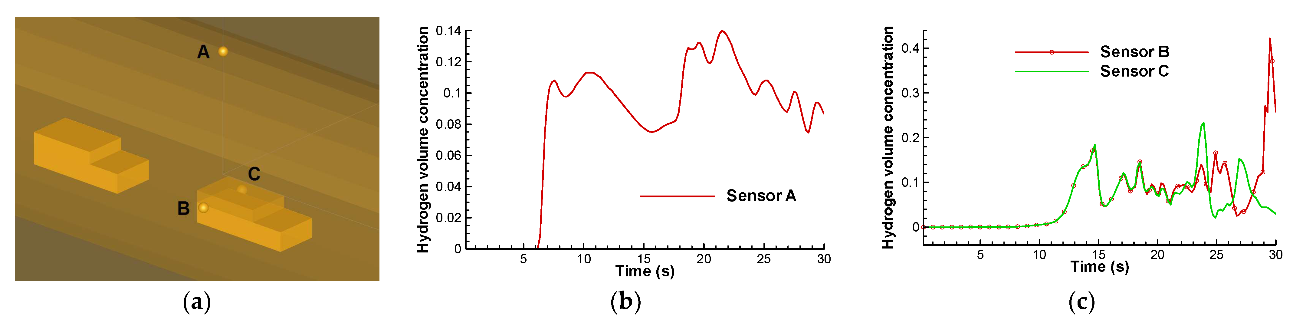
During the simulations, several “sensors” of field variables were placed at chosen positions. In Figure 7, the concentration time series of three sensors are presented. Sensor A is placed at 0.1 m from the top of the tunnel. Its coordinates are (0, 0, 5). Sensors B and C are at symmetrical positions at 0.2 m from the sides of the car, at 1 m from the street, with the coordinates (0, −1.1, −1) and (0, 1.1, −1), respectively (Figure 7a).
From Figure 7b, we can notice that there are two different periods of high concentrations: one around 10 s and another one at about 20 s. Even if this sensor is above the back of the car, the first cloud that it detects is in fact hydrogen that originates from the front of the car. Hydrogen first reaches the ceiling at about X = 3.3 m through the two front columns seen in Figure 6g and starts spreading along the crown of the tunnel towards both directions. The part of this cloud that is directed towards sensor A (left direction) is responsible for the first local peak value of around 11% vol. at 10.5 s. While the propagation front of this cloud moves away towards the left, the concentrations at sensor A drop. In the meantime, the cloud from the two back columns of hydrogen (Figure 6g) arrives at sensor A, and at about 21.5 s, we have the maximum concentration of 14% vol. due to the combined influence of the unified four columns of hydrogen.
The plane XZ at Y = 0 is a symmetry plane of the problem and sensors B and C are symmetric. We notice that their calculated concentration values are identical till the time of 17 s (Figure 7c), but after the time of 20 s, their values are completely different. This reminds us of the chaotic nature of the Navier–Stokes equations and is due to the fact that the flow of our problem is very unsteady, as it involves both very high velocities and buoyant effects. The unsteady nature of such problems can be very easily noticed at the instantaneous concentration isosurfaces in the figures of Huang et al. [32], who performed an LES study. The URANS methodology we have used can also capture some large scales of unsteady phenomena [46,61], as in our case.
Figure 7.
Results from three sensors: (a) positions of the sensors A, B and C; (b) hydrogen volume concentration time series for sensor A; (c) hydrogen volume concentration time series for sensors B and C.
Figure 7.
Results from three sensors: (a) positions of the sensors A, B and C; (b) hydrogen volume concentration time series for sensor A; (c) hydrogen volume concentration time series for sensors B and C.

Figure 7c reveals the stochastic nature of the flow that demands caution about how we should use and interpret the results of the simulations. In order to obtain safer conclusions from such simulations, a good practice is to first look at the general flow features and try to understand what are the possible physical phenomena that can occur and not what are the exact values of the variables at specific points. It is better to look at the results first qualitatively and then quantitatively. Any comparison with the experimental sensors’ values, for example, could be performed only after a detailed examination of the flow field and possible determination of the prevailing phenomena that may influence the measurements. The values of sensors in areas with high gradients of the variables might vary between two different realisations of the same experiment or between two different simulations that have (slightly) modified parameters. This should be taken into account when positioning the experimental sensors.
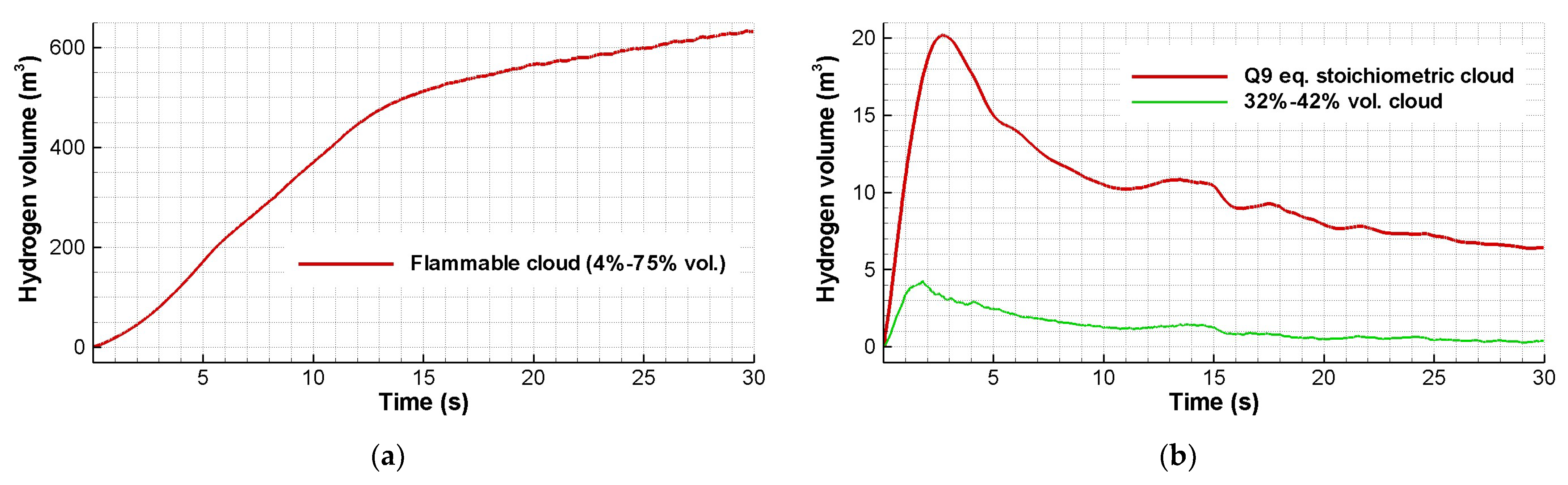
The total volume of the flammable cloud and the total equivalent stoichiometric cloud size Q9 inside the whole tunnel are more “global” values to characterise the results of the simulation. The Q9 cloud is defined in [19] and can be considered as “a scaling of the non-homogeneous gas cloud to a smaller stoichiometric gas cloud that is expected to give similar explosion loads as the original cloud (provided conservative shape and position of cloud, and conservative ignition point)”. These values also have a practical meaning, as they represent a level of hazard.
The flammable cloud volume (Figure 8a) increases almost linearly till about 13 s, when it reaches the value of 470 m3; then, its increase rate declines. The maximum flammable volume in the tunnel of 200 m is 663 m3 and is attained 41 s after the start of the release. As we can see from Figure 6, most of the flammable cloud is gathered along the area of the ceiling, with total lengths there of about 20.6, 33.8 and 44.8 m at 10, 15 and 20 s, respectively. After the time that hydrogen reaches the ceiling, the average concentration there till the time of 30 s is of the order of a 9% vol. for sensors along the central area of the tunnel (see also Figure 7b).
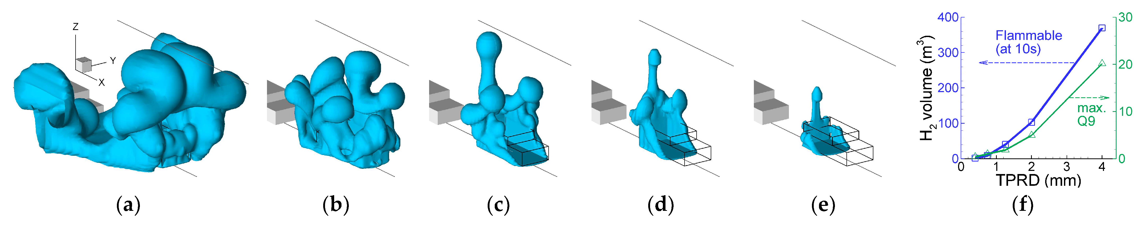
Concerning the potential hazards, the examination of the equivalent stoichiometric cloud volume Q9 (Figure 9b) is considered more appropriate than that of the flammable cloud [19], as higher Q9 values mean more damage in cases of ignition. From Figure 8b, we see that the maximum Q9 is 20.2 m3 and occurs at 2.7 s, when almost all the hydrogen is still around the car. In Figure 8b, there is also a thinner green line that represents the evolution of the 32–42% vol. hydrogen cloud, which, in general, follows the trends of the Q9 line, but with much lower values. The maximum in this case is 4.3 m3, occurring at 1.8 s. The concentration range of 32–42% vol. is considered a very dangerous one, almost as dangerous as the 25–35% vol., which is around the stoichiometry.
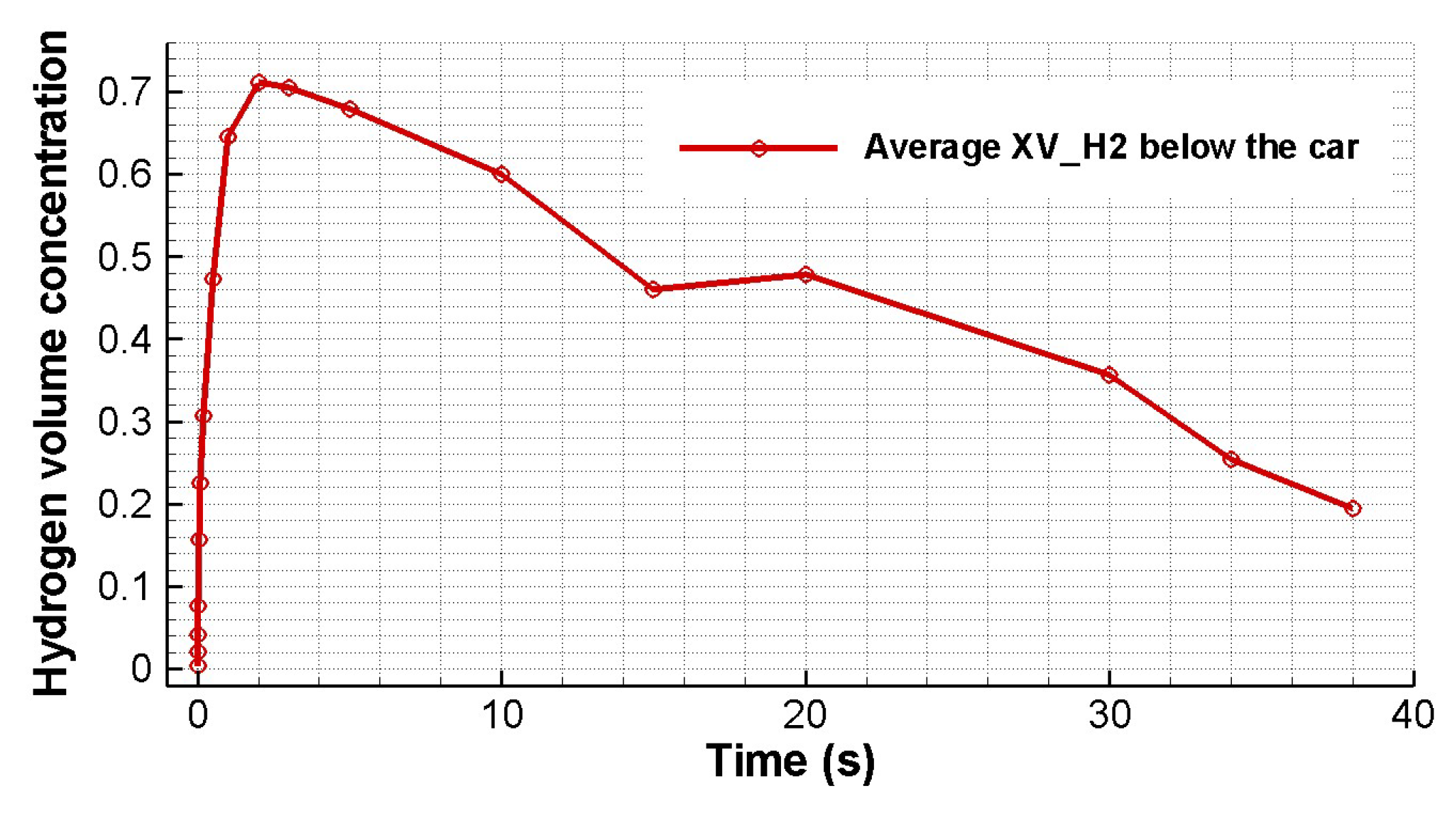
In Figure 9, the average hydrogen volume concentration below the car (i.e., from X = −0.5 till X = 3.7 m, from Y = −0.9 m till Y = 0.9 m and from Z = 0 m till Z = 0.2 m) is presented. According to the results of the simulations, it increases rapidly until a value of 71% vol. is achieved, 2 s after the start of the release. Then, it drops more-or-less linearly, having a value of about 19% vol. at 38 s. We see that the average concentration below the car remains high, due to the hydrogen supply. The irregularity around 15 s is due to the street-level backflow effect at the front of the car.
Figure 8.
Evolution of the total hydrogen cloud volumes inside the tunnel: (a) flammable cloud; (b) equivalent stoichiometric cloud volume Q9 (red) and 32–42% vol. cloud volume (green).
Figure 8.
Evolution of the total hydrogen cloud volumes inside the tunnel: (a) flammable cloud; (b) equivalent stoichiometric cloud volume Q9 (red) and 32–42% vol. cloud volume (green).

Figure 9.
Time evolution of the average hydrogen volume concentration in the area below the car.

In the following subsections of Section 3, the influence of various physical and numerical parameters on the results will be discussed. One of the outcomes of these additional simulations will be the determination of how “global” the physical mechanisms described in this section are. We will focus mainly on the “fresh-air entrainment effect” at the back of the car, the creation of the hydrogen tongues/blisters at the sides of the car and the street-level backflow at the front of the car. These three phenomena are very easily identifiable, as follows:
- I.
- The fresh-air entrainment effect:
- (a)
- With the characteristic “V” shape of chosen isosurfaces below the back of the car (Figure 6b,d);
- (b)
- With the velocity vectors below the car that show an air entrainment (red circle in Figure 4g);
- (c)
- With the centre of the below-car recirculation vortex being transferred out of the limits of the chassis, as in Figure 4e (in case this does not happen, we talk about a “weak fresh-air entrainment”);
- (d)
- With chosen streamlines that show fresh air from the back (or sides) of the car entraining just below the chassis towards the jet (Figure 6b);
- (e)
- With the high difference in hydrogen concentration values just below the car between the side of the entrainment (i.e., back of the car) and the opposite side. For example, in Figure 5e,g, the concentrations at the side of the entrainment (left of the jet) are about 10 times lower than those on the other side (right of the jet);
- II.
- The blisters:
- III.
- The street-level backflow at the front of the car:
- (a)
- With the examination of the velocity vectors below the front of the car that show an air entrainment at the street level at chosen times (insets of Figure 6c,e) and a flow towards the back of the car;
- (b)
- With the examination of streamlines, which shows a street-level flow from outside the limits of the car moving below the vehicle (Figure 6h);
- (c)
- With the high difference in concentration values at the front of the car between the area just below the chassis and the street-level area (inset of Figure 6e,g): concentrations can be over 10 times lower at the street level.
3.2. Sensitivity Tests on Physical Parameters
In this subsection, we will examine slightly modified physical problems from those of the base case in order to see what the main effect will be on the results and on the conclusions reached in Section 3.1.
3.2.1. TPRD Diameter of 2 mm or Smaller
In the case of a TPRD of 2 mm, the initial Reynolds number is about 420,000 and the initial mass flow rate of hydrogen is about four times smaller compared to the case with the TPRD of 4 mm (Figure 2a). Thus, during the first seconds of the release, which are the most critical, the hazard is smaller. However, the release lasts for about 400 s instead of 100 s (Figure 2).
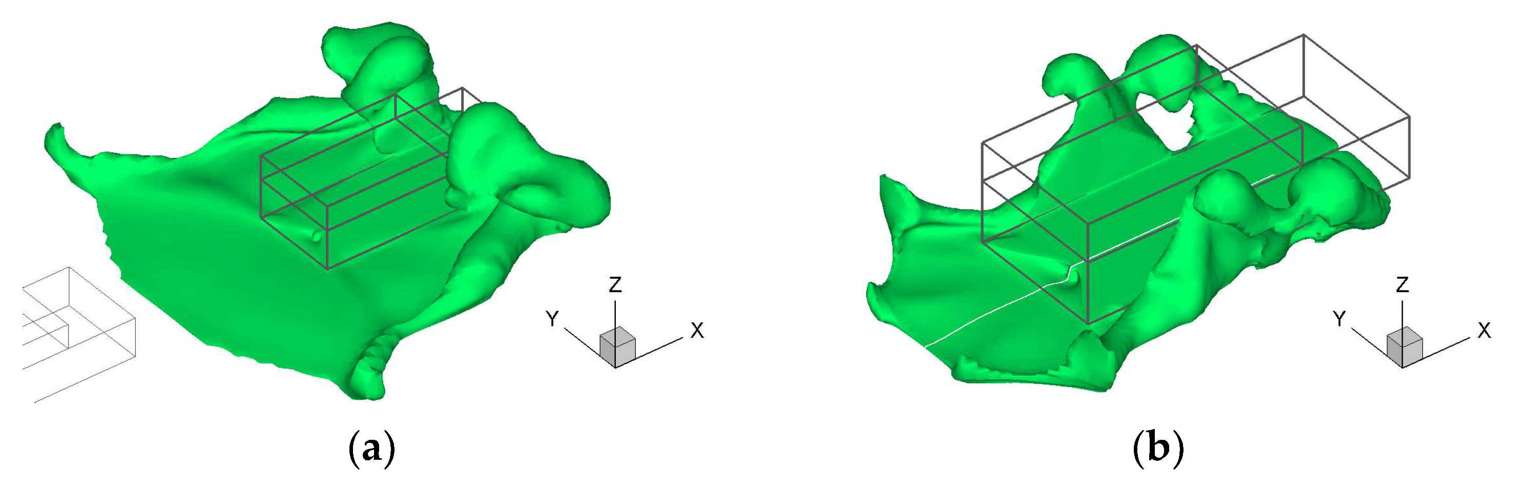
The simulations in this case are performed for the full length of the tunnel (200 m) with the use of symmetry boundary conditions at the Y = 0 plane, and thus half of the domain is modelled. With the use of symmetry boundary conditions, we may lose some of the physics that have to do with the unsteadiness of the flow, but we reduce the computational time by half. The maximum equivalent stoichiometric cloud volume Q9 of the whole tunnel occurs at 3.9 s and is about 5 m3 (i.e., four times smaller than that of the case with the TPRD of 4 mm). For this reason, the TPRD of 2 mm is considered to be generally safer than that of 4 mm. The total flammable cloud is not that smaller though; its maximum is 424 m3 and it appears at a time of 76 s. At the time of 10 s, its value is 103 m3 with a total length at the ceiling of 12.4 m, compared to 369 m3 and 20.6 m, respectively, in the 4 mm TPRD case. The average hydrogen volume concentrations below the car have a maximum of 60%, which occurs at 10 s (i.e., much later than in the 4 mm TPRD case). The 25% vol. hydrogen isosurface at the time of 2 s is presented in Figure 10b.
The “fresh-air entrainment effect” appears again at the back of the car, as can be seen from the characteristic “V” shape formed from the isosurface in Figure 10b below the car. At the two tips of the “V”, two hydrogen tongues appear, like in the 4 mm TPRD case. At the front and at the sides of the car now, four smaller blisters are formed instead of the two large ones that were formed in the 4 mm TPRD case. If we compare Figure 10b with Figure 10a, we see that, in the 4 mm TPRD case, the hydrogen has a wider horizontal spread due to its higher mass flow rate. Also, in Figure 10b, we see that the tongues/blisters that transfer hydrogen upwards are much closer to the car.
The street-level backflow at the front of the car that was commended in Figure 6 of the base case is present in the 2 mm TPRD case also (not shown here). In this case, the backflow starts a few seconds later, is weaker, propagates slower and lasts longer. It plays an important role in the structure of the flow field below the car and, after the time of 40 s, it delimits the recirculation that is created from the source jet.
We see that all the main physical phenomena that are present in the case with the TPRD of 4 mm are also present in the case with the TPRD of 2 mm, but less pronounced, due to the smaller initial flow rate. This is the most important reason that we chose the 4 mm TPRD case as our base case. Another reason is that the 4 mm TPRD case requires a smaller number of cells and decreased computational time, and thus more parametric studies can be performed.
Cases with smaller TPRDs were also tested, namely, with diameters of 1.26 mm, 0.75 mm and 0.4 mm, corresponding to initial mass flow rates of 10%, 3.55% and 1% of those of the base case and covering initial Reynolds numbers between 80,000 and 270,000. These simulations were performed till the time of 10 s, at the 80 m long part of the tunnel. Even if the grid of these additional cases is not very detailed, the discretisation of each of the sources is again four cells. The flammable cloud at 10 s drops to about 40 m3, 9 m3 and 2 m3 and the maximum Q9 cloud is about 1.8 m3, 1 m3 and 0.4 m3 in the 1.26 mm, 0.75 mm and 0.4 mm cases, respectively (Figure 11f).
In Figure 11a–e, the flammable isosurfaces five seconds after the start of the release are shown for each TPRD case. The smaller flow rates result in reduced horizontal spreading above the street, and thus the blister-like structures that transfer hydrogen upwards are much closer to the car. For very small source flow rates, hydrogen sheets are formed at the sides and back of the car and blisters are developed above the sheets (Figure 11c–e). Also, hydrogen recirculations below the car may be too small to reach the end of the chassis and thus the “fresh-air entrainment effect” is weaker. In the simulations mentioned here, it could marginally be noticed in the 1.26 mm case, while it was absent in the smaller TPRD cases. Finally, the street-level backflow at the front of the car could be identified only in the 1.26 mm case. These results should be confirmed in future studies with finer grids.
3.2.2. No-Car Case
In this case, instead of the front car, there is only one very small obstacle that contains the source area, and the second car does not exist. The removal of the cars changes the flow field significantly. In this case, the hydrogen propagation above the street is circular, forming a torus that reaches the sides of the tunnel 2 s after the start of the release. The torus is slightly thicker at four points—at directions diagonal to the grid—due to numerical inaccuracies. Hydrogen is transferred towards the ceiling mainly through the sides of the tunnel. At 10 s, the flammable cloud is 427 m3—slightly bigger than in the base case—with a total length at the ceiling of 19 m. The maximum Q9 cloud occurs at 30 s and is 7.28 m3, with a tendency to increase.
3.2.3. Wheels Added to the Car
The main effect of the presence of wheels is that hydrogen does not propagate horizontally at the place where the wheels are (Figure 12). Hydrogen that does not escape from there is transferred towards the front sides of the car and reinforces the two front blisters.
The fresh-air entrainment effect at the back of the car and, later, the street-level backflow at the front are clearly present in this case too. Side air entrainments below the car are not noticed, due to the back wheels. At 10 s, the flammable cloud is 375 m3, with a total length at the ceiling of 22.1 m. The maximum Q9 cloud occurs at 2.9 s and is 16 m3.
3.2.4. Greater Distance of the Car from the Street
In this case, the car is 0.4 m above the street instead of the 0.2 m in the base case. The flow field looks like a blending of the flow fields of the base case with that of the no-car case. The street-level propagation of the hydrogen cloud is bigger than in the base case and it reaches the second car and the sides of the tunnel. The “fresh-air entrainment effect” is present again, but the back blisters that are formed are weaker compared to those of the base case. The front blisters are transferred towards the front of the car, from where a substantial amount of hydrogen escapes towards the ceiling. The fresh-air entrainment from the sides of the car is more pronounced. At the back of the car, hydrogen reaches the ceiling through the sides of the tunnel. The street-level backflow at the front of the car also appears, but after the time of 15 s. At 10 s, the flammable cloud is 375 m3. The maximum Q9 cloud occurs at 3.1 s and is 13.3 m3. The average hydrogen volume concentrations below the car have an absolute maximum of 31%, which occurs at 15 s, and a local maximum of 28%, which occurs at 1 s.
3.2.5. Other Positions of TPRD
Two additional TPRD distances from the back of the car were tested, namely, 1 m and 1.5 m, instead of 0.5 m that was used in the base case. In the 1 m case, three fresh-air entrainments are present: two from the sides of the car—which are at a distance of 0.9 m from the source—and one, slightly weaker, from the back. In the 1.5 m case, only the side entrainments are present. In both cases, four blisters are formed at the limits of the air entrainments’ dominance, as in the base case. The street-level backflow at the front of the car is again present. The average concentrations below the car have maximums of 64% and 71% for the 1 m and 1.5 m cases, respectively, at 2 s for both cases (i.e., at the same time as in the base case). For both the 1 m and 1.5 m cases though, the average concentrations below the car after the time of 15 s are from 20% to 45% higher, compared to those of the base case. At 10 s, the flammable cloud is 363 m3 and 360 m3 for the 1 m and 1.5 m cases, respectively, with total lengths at the ceiling of 23.4 and 23.7 m, respectively. The maximum Q9 cloud occurs at about 2.75 s and is about 22.28 m3 for both cases.
3.2.6. Different Widths of the Car
In case the width of the car is 1.2 m instead of 1.8 m, except for the fresh-air entrainment effect from the back of the car, the side air entrainments are also strong. As a result, the two back blisters are transferred at higher distances from the source, while the two front blisters are pushed forward and are closer to the vehicle’s sides. This results in the delayed start of the street-level backflow at the front of the car. At 10 s, the flammable cloud is 377 m3, with a total length at the ceiling of 22.1 m. The maximum Q9 cloud occurs at 2.45 s and is 16.5 m3. The average hydrogen volume concentrations below the car have a maximum of 76%, which occurs at 2 s.
A case with an extreme car width of 2.8 m was also tested. Even in this case, the fresh-air entrainment effect is once more dominant at the back of the car, until its corners, where the back hydrogen blisters are formed. The front blisters and the street-level backflow are also present.
3.2.7. Other Roughness of the Solid Objects
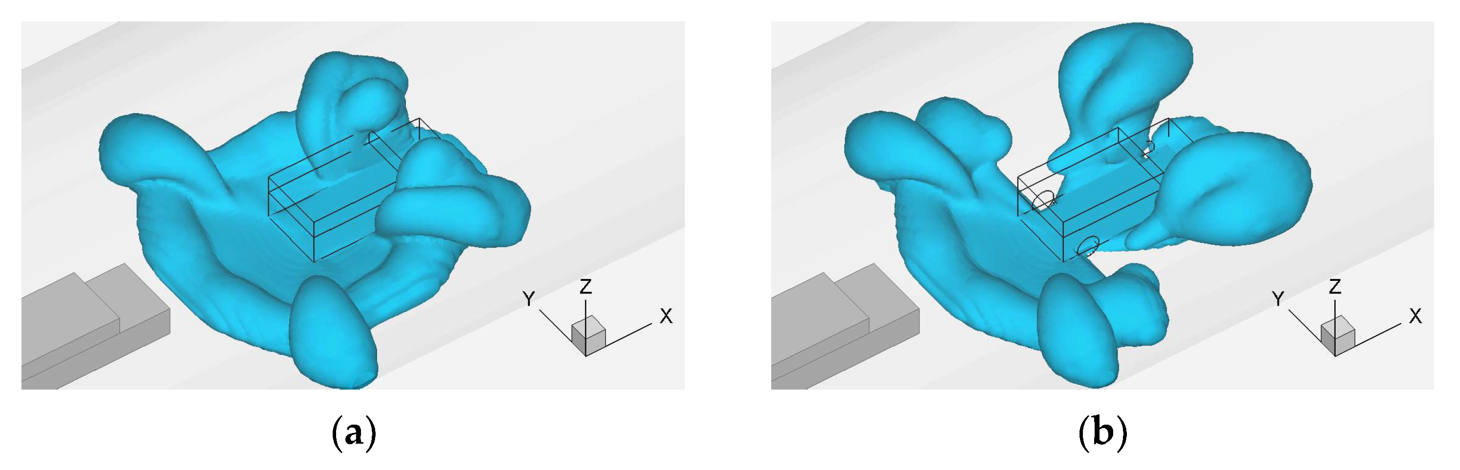
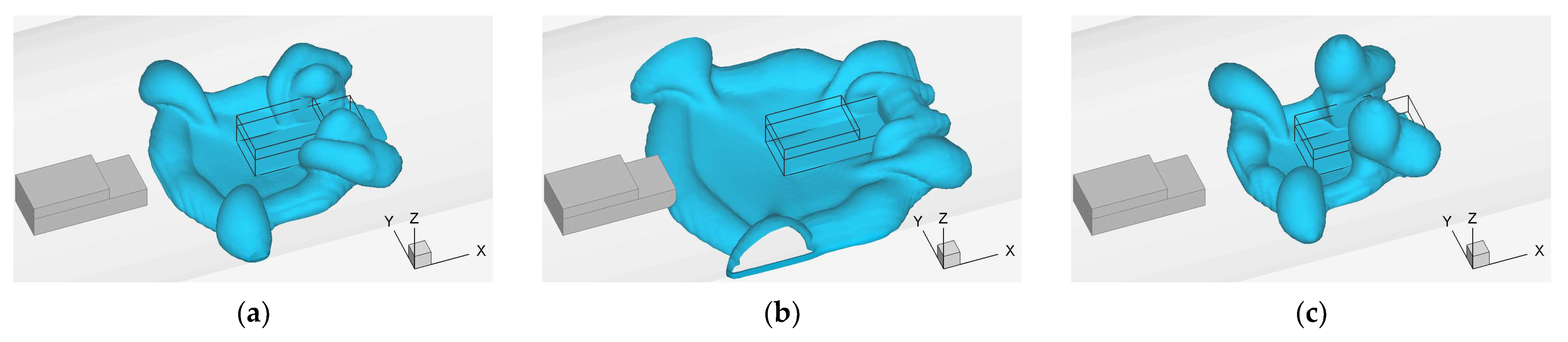
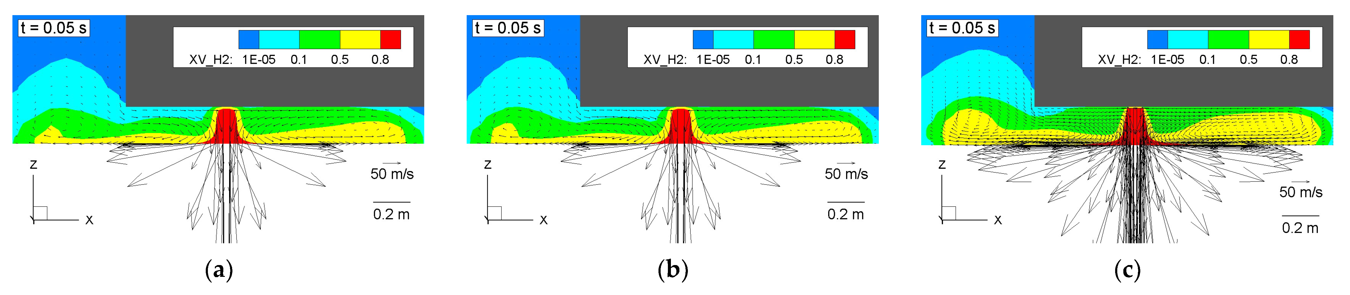
In the base case, a typical roughness of z0 = 0.001 m is considered. Here, two additional roughness values were tested: a ten-times-lower one (0.0001 m) and a two-times-higher one (0.002 m). In each case, the same roughness was applied to all solid surfaces. As seen in Figure 13, the simulation results noticeably depend on the roughness.
All the important physical phenomena that were mentioned at Section 3.1, like the fresh-air entrainment at the back of the car, the creation of the two blisters behind the back corners of the vehicle, the weak side air entrainments, the two complex blisters at the sides of the car and the street-level backflow from the front of the car, are present in all cases. There are some differences though. For example, in the case of smooth solids, a lot of hydrogen escapes from the front of the car (Figure 13b) and that part of the cloud is the first to reach the ceiling, in contrast to the other cases. Due to this, the street-level front backflow is delayed for several seconds. In the same case, we can see that the cloud reached the second car and also spread below it. At 10 s, the wide spreading results in hydrogen being transferred towards the ceiling through the sides of the tunnel. In contrast, in the case of high roughness, at 10 s, the cloud is wrapped around the car, forming a thick hydrogen column up to the ceiling. The flammable volumes at 10 s is 353 m3 and 341 m3 for the z0 = 0.0001 m and z0 = 0.002 m cases, respectively, with total lengths at the ceiling of 22.1 m and 22.5 m, respectively. The maximum Q9 clouds are 16.1 m3 at 3.6 s for the z0 = 0.0001 m case and 20.8 m3 at 2.7 s for the z0 = 0.002 m case. The average hydrogen volume concentrations below the car have maximums of 60% at 1s and 69% at 2 s for the z0 = 0.0001 m and z0 = 0.002 m cases, respectively.
The high speed of the flow above the street makes the roughness of the street play a critical role in the dispersion of hydrogen. Also, the roughness below the car is important, because, for example, a high roughness there blocks the propagation of the cloud towards the front of the car, as can be seen in Figure 13c. Finally, at later stages, the roughness of the ceiling also plays a role in the dispersion of hydrogen and the formation of the flow field there. In simulations of real cases, these three roughness lengths (and especially that of the street) should be estimated with accuracy, something that is not always easy and might be a source of uncertainty.
We can notice that most of the physical mechanisms described in Section 3.1 (like the “fresh-air entrainment effect”, the blisters and the street-level backflow at the front of the car) are, in general, present, even if we modify the physical problem examined. It should be added here that, in the simulations of another study by the authors [62] that focused on hydrogen dispersion in tunnels of various longitudinal slopes and ventilation speeds, the above-mentioned physical mechanisms were, in general, also present.
3.3. Numerical Sensitivity Studies
In this subsection, the effect of several numerical parameters on the results will be discussed.
3.3.1. Convective Numerical Scheme
In Section 2, the reasons for choosing the MUSCL numerical scheme for the discretisation of the convection terms were briefly discussed. Here, we will see how the results change if we use the Fromm scheme instead, which also presents very good behaviour in impinging jets. An additional simulation was performed with the use of the Fromm scheme for the equations of the velocity components, while for the equations of k, ε and the concentrations, the bounded version of the Fromm scheme was applied.
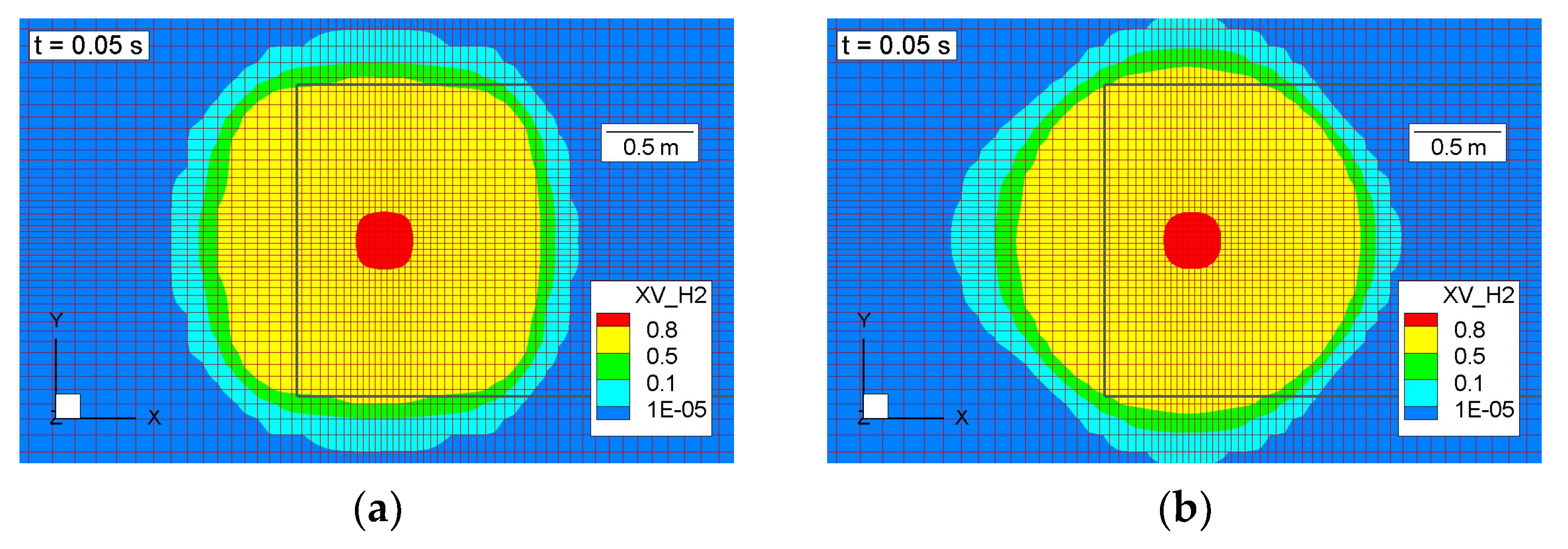
In Figure 14, the results at the early stages of the impingement are presented and compared with those of the base case.
The first remark regarding Figure 14 is that the results of the MUSCL and Fromm schemes are very similar. We can notice though that the high-concentration contours in Figure 14b are more circular. On the other hand, they present a slight tendency towards propagation in a “cross” shape (i.e., aligned to the grid directions). These results are in line with those of Tolias and Venetsanos [50].
From Figure 14, we can see that the low-concentration contours are slightly stretched along the directions of the grid expansion mainly in the case of the Fromm numerical scheme. It should also be noted that the MUSCL simulation presents smoother convergence (not shown here), even if, in some tests, higher errors in the k and ε equations might be noticed when using the MUSCL scheme.
Figure 14.
Hydrogen concentration contours at the street level at 0.05 s: (a) with MUSCL numerical scheme (base case); (b) with Fromm numerical scheme.
Figure 14.
Hydrogen concentration contours at the street level at 0.05 s: (a) with MUSCL numerical scheme (base case); (b) with Fromm numerical scheme.

The physical phenomena that are commented on in the base case are also present in the simulation with the Fromm scheme. The strong fresh-air entrainment effect from the back of the car results in the creation of the back blisters at the corners of the car and, along with the weak side air entrainments, helps in the creation of the two front blisters, which are slightly closer to the car compared to the base case. The differences between the Fromm and the MUSCL cases have mainly to do with the slight tendency of the Fromm scheme to propagate along a “cross” shape in contrast to the slight tendency of the MUSCL to have higher concentrations along the “X” shape. Thus, more hydrogen escapes from the front of the car in the Fromm case, and the street-level backflow there starts a few seconds later than in the base case. The maximum Q9 cloud in the Fromm case is 21.7 m3 compared to the 20.2 m3 in the base case. The average hydrogen volume concentrations below the car have a maximum of 70%, which occurs at 1 s. At later times, the cloud propagation along the ceiling is more or less the same. At 10 s, the flammable cloud is 369 m3 for both cases. It should finally be noted that test simulations with finer grids and a 16-cell discretisation of the source revealed that, as the grids become denser, the differences between the Fromm and MUSCL schemes vanish.
Regarding the false effects of the numerical scheme on the results, several tests performed during this work revealed that these effects are stronger in confined impinging jets (compared to unconfined ones), in coarser grids and at higher mass flow rates (bigger TPRD diameters). It should be noted that the existence and the approximate size of the four blisters seen in Figure 6b are not influenced by the choice of the numerical scheme. A final note is that, in case the Cartesian grid is not aligned with the car (or any other solid that confines the impingement) direction, the use of the Fromm scheme is suggested, as a simulation performed with the use of the MUSCL scheme in an oblique car case (i.e., same TPRD position but with the axis of the car forming a 30-degree angle with the symmetry plane of the tunnel) resulted in the creation of two additional false blisters.
3.3.2. Grid
Several grids were tested. In Figure 15, the results of three of them are presented. The first one is that of the base case and has a resolution of four cells at the source and a total resolution of 171 × 84 × 50 cells in the X, Y, Z directions, respectively. The second one (Figure 15b) is much more uniform, especially at the area around the first car, and has a resolution of 209 × 112 × 50 cells. The third one has an increased resolution of 16 cells at the source and 193 × 110 × 58 total cells, from which half are resolved, due to the use of the symmetry boundary condition in the Y direction. The three grids are named as “base”, “uniform” and “fine”, respectively. A fourth grid with 16 cells at the source and 271 × 210 × 66 total cells (“fine-uniform”) was also tested, but its results are almost the same as those presented for the “fine” grid (Figure 15c) and thus are not included here. Further refinement of the grid is not believed to affect the results and has no meaning if the notional nozzle approach is followed.
As can be seen from Figure 15a,b, the effect of the uniformity of the grid is minor. The contours are almost the same, and the hydrogen blisters that are formed in the case of the uniform grid are at the same place and with the same size as in the base case. A closer look at Figure 15a,b though reveals some small differences in the shape of the recirculation/torus behind the car that are generally strengthened as the time passes. Such small differences finally mildly affect the hydrogen dispersion at the ceiling. For example, at sensor A (Figure 7a), the first two local maximums (Figure 7b, around 10 s) are unified to one in the case of the uniform grid, with a peak value close to 0.14 instead of around 0.12 in the base case. Such differences are to be expected at such unsteady flows. In the uniform grid case, the flammable cloud at 10 s is 373 m3, the maximum Q9 is 20.4 m3 at 2.5 s and the average concentrations below the car have a maximum of 71%, which occurs at 2 s, values which are almost the same with those of the base case.
The resolution of the source has a more severe effect on the results. In Figure 15c, we see that the hydrogen concentrations within the recirculation vortices are generally higher than those of the base case (Figure 15a). This is partly due to the fact that the horizontal velocities close to the impingement point are higher (Figure 15c) due to the finer resolution of the grid at the Z axis. Thus, more hydrogen is transferred horizontally. The bigger difference between the base and the fine grid though is the fact that in the fine-grid case, the recirculations have at their outer limits a stronger upwards-velocity component and thus are slightly “detached” from the ground there. At later times, this behaviour results in worth-mentioning differences in the flow field. For example, behind the car, more hydrogen is transferred upwards, and an additional blister is formed there. It is believed that the differences between the fine and base grids are mainly due to the fact that in the fine-grid case, the recirculations are better resolved.
Concerning the strong fresh-air entrainment effect at the back of the car, it is also present in the case of the fine grid and affects the flow field below the car. The flow around the car in this case is more detailed and one additional blister at each side of the car can be identified, between the back and the front blisters of the base case. The street-level backflow at the front of the car is present, as in the base case, even if it starts a few seconds later due to the different flow fields. The hydrogen cloud is generally closer to the car than in the base case. At 10 s, the columns that transfer hydrogen upwards (commented on in Figure 6f) have already been unified to one thick column that surrounds the whole car. Concerning the flammable volume, the values of the base- and fine-grid cases are the same till 7.5 s, and then they start deviating. At 10 s, the flammable cloud of the fine-grid case is 328 m3, while the maximum Q9 cloud occurs at 2.6 s and is 21.5 m3. The average hydrogen volume concentrations below the car have an absolute maximum of 82%, which occurs at 7 s, and a local maximum of 78% at 1 s.
Several tests were performed with coarser grids also, with only a one-cell resolution of the source. In all these cases, and regardless of the density of the grid, the cloud below the car propagates at preferred directions and not circularly. In the case of the MUSCL scheme, an “X” shaped, butterfly-like cloud is formed, while in the case of the Fromm scheme, a cross-shaped cloud is formed. Thus, the one-cell source resolution is inadequate and does not provide the correct flow below and around the car, even if effects like the fresh-air entrainment from the back may still be present. It is interesting that if we remove the car (like in Section 3.2.2), then the cloud propagation is more circular (forming a square with rounded corners in the MUSCL case and a rhombus with rounded corners in the Fromm case). This means that the confined impinging jets are more demanding than the unconfined ones concerning the accuracy of the numerical scheme. Despite the fact that the flow field is not solved correctly close to the source, the cloud propagation inside the tunnel away from the car is similar to that of the base case, as the same amount of hydrogen enters the flow domain. At 10 s, the flammable cloud in the case of the uniform coarse grid with the MUSCL scheme is 355 m3, while the maximum Q9 cloud occurs at 2.6 s and is 17.9 m3.
A fine grid with a 16-cell source resolution was also tested in the case of a TPRD of 2 mm. The recirculation vortices below the car again had a slightly different, “detached” shape compared to those of the case with the four-cell source resolution. The different recirculations affected mainly the flow behind the car. The increased hydrogen accumulation there resulted in a cloud much closer to the car than in the four-cell-resolution case. This severely degraded the fresh-air entrainment effect at the back of the car, both regarding its intensity and duration. The street-level backflow at the front is present in both grids. The fine grid of the 2 mm case results in a flammable cloud at 10 s of 125 m3 (compared to 103 m3 of the normal grid), and a maximum Q9 cloud of 5.1 m3 at 15.9 s (compared to 5.0 m3 at 3.9 s). Both grids result in a maximum 25–35% vol. cloud of about 1.6 m3 at about 2 s. One more grid was tested, having a four-cell resolution of the source in the X and Y directions, but a fine grid in the Z direction below the car (the same as that of the fine-grid case). The recirculations and more generally the flow in this case are much closer to those of the fine grid than to those of the normal grid. This means that if the resolution of the source area is adequate (i.e., at least four cells) and there are limited computational resources, then a denser grid close to the source in the Z direction is preferred instead of in the X and Y directions. As a rule of thumb, at least a dozen cells below the car are needed if we want to adequately solve the recirculations in cases similar to those examined in this work.
3.3.3. Source Mass Flow Reduction Method
In the simulations mentioned so far, the blowdown of emitted hydrogen was practically achieved with a method equivalent to reducing the source boundary velocity component (w). In reality though, the emission velocity does not drop and remains sonic until almost all of the hydrogen is emitted. In order to assess the effect of this, an alternative way of simulating the decreasing mass flow rate was tested by reducing the “emitting” surface with time and having constant velocity. Thus, the momentum of the jet was equal to the actual one.
In this case, the results show that the hydrogen cloud propagation is practically the same as that of the base case till the time of 1 s, and all the physical phenomena reported in Section 3.1 are present. Then, the jet and impingement velocities are higher than those of the base case and they slowly start affecting the dispersion. The maximum Q9 cloud occurs at 2.8 s and is 19.7 m3, and the average hydrogen volume concentrations below the car have a maximum of 68% at 2 s, values that are very close to those of the base case. After the time of 5 s (when the source mass flow rate has already dropped by 46.5%), the differences regarding the hydrogen dispersion start to become worth mentioning. In general, the horizontal spreading above the street is stronger, the low-concentration areas bigger and the high-concentration areas smaller.
At the time of 10 s, the four hydrogen columns that correspond to those of the inset of Figure 6f are closer to the tunnel sides and have about double distances among them compared to the base case. The flammable cloud at this time is 388 m3 and its length at the ceiling is 18.9 m. At the time of 20 s, these four columns are still close to the sides of the tunnel and have not merged, in contrast to what happens in the base case (Figure 6h). Thus, there is also a flammable cloud at the sides of the tunnel. At 20 s, its total volume is 607 m3 and its length at the ceiling is 40.9 m (compared to 566 m3 and 44.8 m in the base case, respectively).
A case with a fine uniform grid with a reducing emitting surface was also tested, with a resolution of 16 cells in the source. In this case, the changes compared to the results of the fine grid with reducing velocity are not as big as in the cases with the base grid. These changes have mainly to do with the slightly wider cloud around the car after the time of 5 s. Even wider, the cloud in this case does not extend along the sides of the tunnel. In this case, the flammable cloud at 10 s is 354 m3 and the maximum Q9 cloud is 20.1 m3 at 2.8 s, and these values are believed to be more correct than those of the base case due to the finer grid and the more accurate representation of the blowdown.
Finally, tests with a reducing emitting surface were also performed for the cases of 2 mm TPRDs, both for normal and fine grids, and the differences are not as big as in the 4 mm cases, due to the reduced mass flow rate of hydrogen at the source.
3.3.4. Values of k and ε at the Source
The choice of the boundary condition regarding the turbulent kinetic energy and its dissipation at the source surface is not straightforward. The “zero gradient” choice of the base case has the advantage of letting the turbulence develop freely from the flow field and it also does not suppress it at the boundaries of the source area. This choice produces relatively high turbulence values. Another choice would be to put given zero values of k and ε at the source (named “zero values” from now on), as the flow at the Mach disk of the notional nozzle is considered to have no turbulence. This case results in much lower turbulence of the jet. A third choice would be to put high given values of k and ε at the source (named “high given values” from now on), in order not to suspend the turbulence of the jet very close to the source (as happens with the “zero values” choice). The values of 10,000 m2/s2 for k and 2500 m2/s3 for ε are chosen, mainly based on the values of k and ε of the “zero values” case a few cells away from the source. Additional simulations for the “zero values” and “high given values” cases were performed.
The results show that this parameter is not very critical. Of course, the turbulent kinetic energy values of the jet close to the source differ, but that does not have a severe effect on the hydrogen propagation. More specifically, in the “zero gradient” and “high given values” cases, the k contours have similar shapes but different values, with maximums inside the core of the jet of about 200,000 m2/s2 for the “zero gradient” case and 70,000 m2/s2 for the “high given values” case (excluding the cells adjacent to the source). In the “zero values” case, the core of the jet has lower turbulence and the high-turbulence regions are formed at its circumference, with typical maximums there of about 30,000 m2/s2.
Regarding the hydrogen propagation, the differences during the first seconds have mainly to do with the higher turbulent kinetic energy values of the “zero gradient” case, which produce, for example, smoother hydrogen isosurfaces than the “zero values” and “high given values” cases. At 10 s, the flammable clouds are 369 m3, 379 m3 and 372 m3 with total lengths at the ceiling of 20.6 m, 20.1 m and 20.1 m for the “zero gradient”, “zero values” and “high given values” cases, respectively, while the maximum Q9 clouds are 20.2 m3, 20.7 m3 and 20.7 m3 at 2.7 s, 2.8 s and 2.9 s, respectively. The average hydrogen volume concentrations below the car have maximums of 71% at 2 s, 70% at 2 s and 71% at 2 s (i.e., values that are practically the same for all three cases).
Each one of the three choices presents advantages and drawbacks, but they all provide more-or-less similar results regarding hydrogen propagation, given the unsteady nature of the particular flow. In case the area very close to the source is of interest, further investigation is needed; otherwise, any of the choices is acceptable. The notional nozzle approach itself imposes more severe assumptions than the choice of the boundary condition of k and ε at the source area.
3.3.5. Turbulence Model
The high-speed recirculations of the flow below the car are very demanding regarding the turbulence model. Thus, a different model was also tested, and more specifically the RNG k-ε. The specific model is derived from the renormalization-group mathematical theory, and it is known for having good behaviour in recirculating flows [63]. The results show that the influence of the turbulence model is not that critical, given the unsteady nature of the flow and the other uncertainties of the simulation. In the case of the RNG k-ε, the horizontal velocities in the impingement region are slightly higher than those of the base case, and the horizontal cloud propagation is slightly wider. The flammable cloud at 10 s is 383 m3 with a length of 19.3 m at the ceiling, while the maximum Q9 cloud is 19.7 m3 at 2.8 s. The average hydrogen volume concentrations below the car have a maximum of 67%, which occurs at 2 s.
4. Conclusions
During the hydrogen release through a TPRD below a car, the main physical phenomenon observed is the “fresh-air entrainment effect”. A few tenths of the second after the start of the release, hydrogen has filled part of the area below the car and starts spreading out of its limits. From the first point that this happens, which, in our case, is the back of the car, fresh air entrains just below the chassis towards the source. This is stronger for higher source mass flow rates and affects the subsequent flow field. Another observed phenomenon is the creation and reinforcement of blister-like structures around the car that constitute the main mechanism of upwards hydrogen convection. Finally, the street-level backflow at the front of the car is a phenomenon that is also observed, a few seconds later. These phenomena are independent of the presence of the tunnel and can be generalised for many confined jets of similar configurations. Their identification may be useful for the design of experiments, for choosing the TPRD characteristics, for potential safety measures and for understanding the further hydrogen cloud propagation.
Concerning the physical parameters that affect the hydrogen dispersion, the most important is the initial mass flow rate, which depends on the diameter of the TPRD. Smaller TPRDs result in smaller hydrogen clouds for longer periods of time. The geometry between the car and the street and the roughness also have relatively big influences on the results and should be modelled in detail.
Regarding the numerical parameters that influence the results, the convective numerical scheme is very critical for Cartesian grids like those used in this study. High-order schemes like “Fromm” or “MUSCL” are needed, combined with at least a four-cell resolution of the source. Even though the Fromm scheme behaves better in the impingement region, the MUSCL scheme was mainly used in this work, as it has the theoretical advantage of being a bounded scheme and thus it is supposed to provide more physical results. The grid is also critical, especially concerning the resolution of the source and the number of cells between the car and the street. In case the computational resources do not allow a high resolution at the source, its discretisation with four cells should be considered as acceptable, especially for studies of hydrogen propagation at the tunnel and not around the car. Regarding the source mass flow reduction method, it is better to have a method that retains the same momentum as the actual source, as this affects the hydrogen propagation after the first seconds of the release, especially for high-mass-flow-rate cases. The boundary conditions of k and ε at the source and the turbulence model used are of secondary importance, especially given the high unsteadiness of the flow and the other physical and CFD uncertainties.
The flow examined in this work is stochastic and thus there is an inherent difficulty regarding its simulation with RANS CFD. Methodologies like LES will not only provide more accurate results but also a deeper and more detailed insight into the physical phenomena that occur in such unsteady and complex flows, and this is interesting for future research. Regarding the flow below the car during the first seconds of the release, it would also be interesting for future studies to compare with experimental results in order to cross-check the physical phenomena observed. It is stressed that measurements from confined jets are needed, because they have different physics than unconfined jets and are more difficult to model. Investigation of the further propagation of hydrogen along the tunnel ceiling for various slopes, both with and without ventilation, is also work that would expand the current study. Finally, it would be useful to compare such CFD results with those of relevant experiments in tunnels.
Author Contributions
Conceptualisation, S.G.G., A.G.V. and N.K.; methodology, A.G.V. and I.C.T.; software, A.G.V., I.C.T. and N.K.; validation, N.K., A.G.V. and I.C.T.; formal analysis, N.K. and I.C.T.; investigation, N.K.; resources, N.K. and I.C.T.; data curation, N.K. and I.C.T.; writing—original draft preparation, N.K.; writing—review and editing, S.G.G.; visualisation, N.K.; supervision, A.G.V. and S.G.G.; project administration, A.G.V. and S.G.G.; funding acquisition, A.G.V. All authors have read and agreed to the published version of the manuscript.
Funding
Part of this research was funded from the Clean Hydrogen Joint Undertaking through grant agreement No 826193 (project HyTunnel-CS). The Joint Undertaking receives support from the European Union’s Horizon 2020 research and innovation programme.
Data Availability Statement
Not applicable.
Acknowledgments
This work was supported by computational time granted from the National Infrastructures for Research and Technology S.A. (GRNET) in the National HPC facility—ARIS—under project ID pr014025 (H2TUN).
Conflicts of Interest
The authors declare no conflict of interest.
References
- Abánades, A. Perspectives on Hydrogen. Energies 2022, 16, 437. [Google Scholar] [CrossRef]
- Mazloomi, K.; Gomes, C. Hydrogen as an Energy Carrier: Prospects and Challenges. Renew. Sustain. Energy Rev. 2012, 16, 3024–3033. [Google Scholar] [CrossRef]
- Abe, J.O.; Popoola, A.P.I.; Ajenifuja, E.; Popoola, O.M. Hydrogen Energy, Economy and Storage: Review and Recommendation. Int. J. Hydrogen Energy 2019, 44, 15072–15086. [Google Scholar] [CrossRef]
- Abdin, Z.; Zafaranloo, A.; Rafiee, A.; Mérida, W.; Lipiński, W.; Khalilpour, K.R. Hydrogen as an Energy Vector. Renew. Sustain. Energy Rev. 2020, 120, 109620. [Google Scholar] [CrossRef]
- Kovač, A.; Paranos, M.; Marciuš, D. Hydrogen in Energy Transition: A Review. Int. J. Hydrogen Energy 2021, 46, 10016–10035. [Google Scholar] [CrossRef]
- Bairrão, D.; Soares, J.; Almeida, J.; Franco, J.F.; Vale, Z. Green Hydrogen and Energy Transition: Current State and Prospects in Portugal. Energies 2023, 16, 551. [Google Scholar] [CrossRef]
- Molkov, V. Fundamentals of Hydrogen Safety Engineering, Part I; bookboon.com (Ventus Publishing ApS): Copenhagen, Denmark, 2012; ISBN 978-87-403-0226-4. Available online: https://bookboon.com/en/fundamentals-of-hydrogen-safety-engineering-i-ebook (accessed on 30 August 2023).
- Molkov, V. Fundamentals of Hydrogen Safety Engineering, Part II; bookboon.com (Ventus Publishing ApS): Copenhagen, Denmark, 2012; Available online: https://bookboon.com/en/fundamentals-of-hydrogen-safety-engineering-ii-ebook (accessed on 30 August 2023).
- Felseghi, R.-A.; Carcadea, E.; Raboaca, M.S.; Trufin, C.N.; Filote, C. Hydrogen Fuel Cell Technology for the Sustainable Future of Stationary Applications. Energies 2019, 12, 4593. [Google Scholar] [CrossRef]
- Bethoux, O. Hydrogen Fuel Cell Road Vehicles and Their Infrastructure: An Option towards an Environmentally Friendly Energy Transition. Energies 2020, 13, 6132. [Google Scholar] [CrossRef]
- Global EV Outlook 2022. Available online: https://www.iea.org/reports/global-ev-outlook-2022 (accessed on 26 June 2023).
- Global Hydrogen Fuel Stations by Country 2022. Available online: https://0-www-statista-com.brum.beds.ac.uk/statistics/1026719/number-of-hydrogen-fuel-stations-by-country (accessed on 7 January 2023).
- Pawelczyk, E.; Łukasik, N.; Wysocka, I.; Rogala, A.; Gębicki, J. Recent Progress on Hydrogen Storage and Production Using Chemical Hydrogen Carriers. Energies 2022, 15, 4964. [Google Scholar] [CrossRef]
- Venetsanos, A.G.; Huld, T.; Adams, P.; Bartzis, J.G. Source, Dispersion and Combustion Modelling of an Accidental Release of Hydrogen in an Urban Environment. J. Hazard. Mater. 2003, 105, 1–25. [Google Scholar] [CrossRef]
- Venetsanos, A.G.; Baraldi, D.; Adams, P.; Heggem, P.S.; Wilkening, H. CFD Modelling of Hydrogen Release, Dispersion and Combustion for Automotive Scenarios. J. Loss Prev. Process Ind. 2008, 21, 162–184. [Google Scholar] [CrossRef]
- Baraldi, D.; Venetsanos, A.G.; Papanikolaou, E.; Heitsch, M.; Dallas, V. Numerical Analysis of Release, Dispersion and Combustion of Liquid Hydrogen in a Mock-up Hydrogen Refuelling Station. J. Loss Prev. Process Ind. 2009, 22, 303–315. [Google Scholar] [CrossRef]
- Papanikolaou, E.A.; Venetsanos, A.G.; Heitsch, M.; Baraldi, D.; Huser, A.; Pujol, J.; Garcia, J.; Markatos, N. HySafe SBEP-V20: Numerical Studies of Release Experiments inside a Naturally Ventilated Residential Garage. Int. J. Hydrogen Energy 2010, 35, 4747–4757. [Google Scholar] [CrossRef]
- Venetsanos, A.G.; Papanikolaou, E.; Hansen, O.R.; Middha, P.; Garcia, J.; Heitsch, M.; Baraldi, D.; Adams, P. HySafe Standard Benchmark Problem SBEP-V11: Predictions of Hydrogen Release and Dispersion from a CGH2 Bus in an Underpass. Int. J. Hydrogen Energy 2010, 35, 3857–3867. [Google Scholar] [CrossRef]
- Middha, P.; Hansen, O.R. CFD Simulation Study to Investigate the Risk from Hydrogen Vehicles in Tunnels. Int. J. Hydrogen Energy 2009, 34, 5875–5886. [Google Scholar] [CrossRef]
- Breitung, W.; Bielert, U.; Necker, G.; Veser, A.; Wetzel, F.J.; Pehr, K. Numerical Simulation and Safety Evaluation of Tunnel Accidents with a Hydrogen Powered Vehicle. In Proceedings of the 13th World Hydrogen Energy Confernce, Beijing, China, 12–15 June 2000. [Google Scholar]
- Mukai, S.; Suzuki, J.; Mitsuishi, H.; Oyakawa, K.; Watanabe, S. CFD Simulation of Diffusion of Hydrogen Leakage Caused by Fuel Cell Vehicle Accident in Tunnel, Underground Parking Lot and Multi-Story Parking Garage. In Proceedings of the 19th International Technical Conference on the Enhanced Safety of Vehicles (ESV), Washington, DC, USA, 6–9 June 2005. [Google Scholar]
- Houf, W.G.; Evans, G.H.; Merilo, E.; Groethe, M.; James, S.C. Releases from Hydrogen Fuel-Cell Vehicles in Tunnels. Int. J. Hydrogen Energy 2012, 37, 715–719. [Google Scholar] [CrossRef]
- Choi, J.; Hur, N.; Kang, S.; Lee, E.D.; Lee, K.-B. A CFD Simulation of Hydrogen Dispersion for the Hydrogen Leakage from a Fuel Cell Vehicle in an Underground Parking Garage. Int. J. Hydrogen Energy 2013, 38, 8084–8091. [Google Scholar] [CrossRef]
- Xie, H.; Li, X.; Christopher, D.M. Emergency Blower Ventilation to Disperse Hydrogen Leaking from a Hydrogen-Fueled Vehicle. Int. J. Hydrogen Energy 2015, 40, 8230–8238. [Google Scholar] [CrossRef]
- Liu, W.; Christopher, D.M. Dispersion of Hydrogen Leaking from a Hydrogen Fuel Cell Vehicle. Int. J. Hydrogen Energy 2015, 40, 16673–16682. [Google Scholar] [CrossRef]
- Bie, H.Y.; Hao, Z.R. Simulation Analysis on the Risk of Hydrogen Releases and Combustion in Subsea Tunnels. Int. J. Hydrogen Energy 2017, 42, 7617–7624. [Google Scholar] [CrossRef]
- Li, Z.; Luo, Y. Comparisons of Hazard Distances and Accident Durations between Hydrogen Vehicles and CNG Vehicles. Int. J. Hydrogen Energy 2019, 44, 8954–8959. [Google Scholar] [CrossRef]
- Li, Z.; Makarov, D.; Keenan, J.; Molkov, V. CFD Study of the Unignited and Ignited Hydrogen Releases from TPRD under a Fuel Cell Car. In Proceedings of the 6th International Conference on Hydrogen Safety, Yokohama, Japan, 19–21 October 2015. [Google Scholar]
- Hussein, H.; Brennan, S.; Molkov, V. Dispersion of Hydrogen Release in a Naturally Ventilated Covered Car Park. Int. J. Hydrogen Energy 2020, 45, 23882–23897. [Google Scholar] [CrossRef]
- Shentsov, V.; Makarov, D.; Molkov, V. Effect of TPRD Diameter and Direction of Release on Hydrogen Dispersion in Underground Parking. In Proceedings of the 9th International Conference on Hydrogen Safety (ICHS2021), Edinburgh, UK, 21–23 September 2021. [Google Scholar]
- Li, Y.; Xiao, J.; Zhang, H.; Breitung, W.; Travis, J.; Kuznetsov, M.; Jordan, T. Numerical Analysis of Hydrogen Release, Dispersion and Combustion in a Tunnel with Fuel Cell Vehicles using All-Speed CFD Code GASFLOW-MPI. Int. J. Hydrogen Energy 2021, 46, 12474–12486. [Google Scholar] [CrossRef]
- Huang, T.; Zhao, M.; Ba, Q.; Christopher, D.M.; Li, X. Modeling of Hydrogen Dispersion from Hydrogen Fuel Cell Vehicles in an Underground Parking Garage. Int. J. Hydrogen Energy 2022, 47, 686–696. [Google Scholar] [CrossRef]
- Hansen, O.R.; Hansen, E.S.; Kjellander, M.T.; Martini, R. CFD Study to Assess Safety Aspects of TPRD Releases from Heavy-Duty Hydrogen Vehicles and Trains in Tunnels. Chem. Eng. Trans. 2022, 90, 91–96. [Google Scholar] [CrossRef]
- Lv, H.; Shen, Y.; Zheng, T.; Zhou, W.; Ming, P.; Zhang, C. Numerical Study of Hydrogen Leakage, Diffusion, and Combustion in an Outdoor Parking Space under Different Parking Configurations. Renew. Sustain. Energy Rev. 2023, 173, 113093. [Google Scholar] [CrossRef]
- Shen, Y.; Zheng, T.; Lv, H.; Zhou, W.; Zhang, C. Numerical Simulation of Hydrogen Leakage from Fuel Cell Vehicle in an Outdoor Parking Garage. World Electr. Veh. J. 2021, 12, 118. [Google Scholar] [CrossRef]
- Venetsanos, A.G.; Papanikolaou, E.A.; Bartzis, J.G. The ADREA-HF CFD Code for Consequence Assessment of Hydrogen Applications. Int. J. Hydrogen Energy 2010, 35, 3908–3918. [Google Scholar] [CrossRef]
- Koutsourakis, N.; Tolias, I.C.; Venetsanos, A.G.; Bartzis, J.G. Evaluation of an LES Code against a Hydrogen Dispersion Experiment. CFD Lett. 2012, 4, 225–236. [Google Scholar]
- Koutsourakis, N.; Venetsanos, A.G.; Bartzis, J.G. LES Modelling of Hydrogen Release and Accumulation within a Non-Ventilated Ambient Pressure Garage Using the ADREA-HF CFD Code. Int. J. Hydrogen Energy 2012, 37, 17426–17435. [Google Scholar] [CrossRef]
- Giannissi, S.G.; Hoyes, J.R.; Chernyavskiy, B.; Hooker, P.; Hall, J.; Venetsanos, A.G.; Molkov, V. CFD Benchmark on Hydrogen Release and Dispersion in a Ventilated Enclosure: Passive Ventilation and the Role of an External Wind. Int. J. Hydrogen Energy 2015, 40, 6465–6477. [Google Scholar] [CrossRef]
- Giannissi, S.G.; Tolias, I.C.; Melideo, D.; Baraldi, D.; Shentsov, V.; Makarov, D.; Molkov, V.; Venetsanos, A.G. On the CFD Modelling of Hydrogen Dispersion at Low-Reynolds Number Release in Closed Facility. Int. J. Hydrogen Energy 2021, 46, 29745–29761. [Google Scholar] [CrossRef]
- Bartzis, J. ADREA-HF: A Three-Dimensional Finite Volume Code for Vapour Cloud Dispersion in Complex Terrain. Commission of the European Communities, 1991; Report EUR 13580 EN. Available online: https://op.europa.eu/en/publication-detail/-/publication/32303175-8a49-43bd-acb0-28e9a13d9c54 (accessed on 30 August 2023).
- Bartzis, J.G.; Venetsanos, A.G.; Varvayanni, M.; Catsaros, N.; Megaritou, A. ADREA-I: A Three-Dimensional Transient Transport Code for Complex Terrain and Other Applications. Nucl. Technol. 1991, 94, 135–148. [Google Scholar] [CrossRef]
- Kovalets, I.V.; Andronopoulos, S.; Venetsanos, A.G.; Bartzis, J.G. Optimization of the Numerical Algorithms of the ADREA-I Mesoscale Prognostic Meteorological Model for Real-Time Applications. Environ. Model. Softw. 2008, 23, 96–108. [Google Scholar] [CrossRef]
- Launder, B.E.; Spalding, D.B. The Numerical Computation of Turbulent Flows. Comput. Methods Appl. Mech. Eng. 1974, 3, 269–289. [Google Scholar] [CrossRef]
- Birch, A.D.; Brown, D.R.; Dodson, M.G.; Swaffield, F. The Structure and Concentration Decay of High Pressure Jets of Natural Gas. Combust. Sci. Technol. 1984, 36, 249–261. [Google Scholar] [CrossRef]
- Argyropoulos, C.D.; Markatos, N.C. Recent Advances on the Numerical Modelling of Turbulent Flows. Appl. Math. Model. 2015, 39, 693–732. [Google Scholar] [CrossRef]
- Tolias, I.C.; Giannissi, S.G.; Venetsanos, A.G.; Keenan, J.; Shentsov, V.; Makarov, D.; Coldrick, S.; Kotchourko, A.; Ren, K.; Jedicke, O.; et al. Best Practice Guidelines in Numerical Simulations and CFD Benchmarking for Hydrogen Safety Applications. Int. J. Hydrogen Energy 2019, 44, 9050–9062. [Google Scholar] [CrossRef]
- FCH2 Education—E-Laboratory. Available online: https://fch2edu.eu/home/e-laboratory/ (accessed on 9 January 2023).
- Koutsourakis, N.; Bartzis, J.G.; Efthimiou, G.C.; Sakellaris, I. CFD Studies of Pollutant Spatial Distribution in a Large Office. Int. J. Environ. Pollut. 2019, 65, 125–148. [Google Scholar] [CrossRef]
- Tolias, I.C.; Venetsanos, A.G. Comparison of Convective Schemes in Hydrogen Impinging Jet CFD Simulation. In Proceedings of the 6th International Conference on Hydrogen Safety, Yokohama, Japan, 19–21 October 2015. [Google Scholar]
- Fromm, J.E. A Method for Reducing Dispersion in Convective Difference Schemes. J. Comput. Phys. 1968, 3, 176–189. [Google Scholar] [CrossRef]
- van Leer, B. Towards the Ultimate Conservative Difference Scheme. II. Monotonicity and Conservation Combined in a Second-Order Scheme. J. Comput. Phys. 1974, 14, 361–370. [Google Scholar] [CrossRef]
- Van Leer, B. Towards the Ultimate Conservative Difference Scheme. IV. A New Approach to Numerical Convection. J. Comput. Phys. 1977, 23, 276–299. [Google Scholar] [CrossRef]
- Waterson, N.P.; Deconinck, H. Design Principles for Bounded Higher-Order Convection Schemes—A Unified Approach. J. Comput. Phys. 2007, 224, 182–207. [Google Scholar] [CrossRef]
- Koutsourakis, N.; Giannissi, S.G.; Tolias, I.C.; Venetsanos, A.G.; Forero, D.; Studer, E. Simulations of Hydrogen Dispersion from Fuel Cell Vehicles’ Leakages Inside Full-Scale Tunnel. In Proceedings of the 10th International Conference on Hydrogen Safety (ICHS2023), Québec, QC, Canada, 19–21 September 2023. [Google Scholar]
- Giannissi, S.G.; Venetsanos, A.G.; Rattigan, W.; Lyons, K. CFD Dispersion Simulations of Compressed Hydrogen Releases Through TPRD Inside Scaled Tunnel. In Proceedings of the 10th International Conference on Hydrogen Safety (ICHS2023), Québec, QC, Canada, 19–21 September 2023. [Google Scholar]
- Tolias, I.C.; Rattigan, W.; Lyons, K.; Koumroglou, V.C.; Venetsanos, A.G. CFD Analysis of Delayed Ignition Hydrogen Releases from a Train Inside a Tunnel. In Proceedings of the 10th International Conference on Hydrogen Safety (ICHS2023), Québec, QC, Canada, 19–21 September 2023. [Google Scholar]
- Behnia, M.; Parneix, S.; Shabany, Y.; Durbin, P.A. Numerical Study of Turbulent Heat Transfer in Confined and Unconfined Impinging Jets. Int. J. Heat Fluid Flow 1999, 20, 1–9. [Google Scholar] [CrossRef]
- Sfeir, A.A. The Velocity and Temperature Fields of Rectangular Jets. Int. J. Heat Mass Transf. 1976, 19, 1289–1297. [Google Scholar] [CrossRef]
- Bejan, A.; Ziaei, S.; Lorente, S. Evolution: Why All Plumes and Jets Evolve to Round Cross Sections. Sci. Rep. 2014, 4, 4730. [Google Scholar] [CrossRef]
- Spalart, P.R. Strategies for Turbulence Modelling and Simulations. Int. J. Heat Fluid Flow 2000, 21, 252–263. [Google Scholar] [CrossRef]
- Koutsourakis, N.; Tolias, I.C.; Giannissi, S.G.; Venetsanos, A.G. Numerical Study of the Effects of Tunnel Inclination and Ventilation on the Dispersion of Hydrogen Released from a Car. In Proceedings of the 9th International Conference on Hydrogen Safety (ICHS2021), Edinburgh, UK, 21–23 September 2021. [Google Scholar]
- Koutsourakis, N.; Bartzis, J.G.; Markatos, N.C. Evaluation of Reynolds Stress, k-ε and RNG k-ε Turbulence Models in Street Canyon Flows Using Various Experimental Datasets. Environ. Fluid Mech. 2012, 12, 379–403. [Google Scholar] [CrossRef]
Figure 1.
Geometry details: (a) tunnel cross section; (b) part of the tunnel with the cars and the release position and direction (inset).
Figure 1.
Geometry details: (a) tunnel cross section; (b) part of the tunnel with the cars and the release position and direction (inset).

Figure 2.
Blowdown details for TPRDs of 4 mm and 2 mm: (a) mass flow rate evolution with time; (b) notional nozzle diameter with time.
Figure 2.
Blowdown details for TPRDs of 4 mm and 2 mm: (a) mass flow rate evolution with time; (b) notional nozzle diameter with time.

Figure 3.
Computational grid for the base case: (a) front view; (b) side view; (c) details of the grid around the release (red) area. Each cell there is 0.034 m × 0.034 m.
Figure 3.
Computational grid for the base case: (a) front view; (b) side view; (c) details of the grid around the release (red) area. Each cell there is 0.034 m × 0.034 m.

Figure 10.
Hydrogen volume concentration isosurface of XV = 0.25 at t = 2 s: (a) base case (TPRD diameter of 4 mm); (b) case with TPRD of 2 mm.
Figure 10.
Hydrogen volume concentration isosurface of XV = 0.25 at t = 2 s: (a) base case (TPRD diameter of 4 mm); (b) case with TPRD of 2 mm.

Figure 11.
Effect of the size of the TPRD diameter: (a) TPRD of 4 mm: XV = 0.04 isosurface at 5 s; (b) TPRD of 2 mm; (c) TPRD of 1.26 mm; (d) TPRD of 0.75 mm; (e) TPRD of 0.4 mm; (f) flammable volume at 10 s and max Q9 values for all TPRDs.
Figure 11.
Effect of the size of the TPRD diameter: (a) TPRD of 4 mm: XV = 0.04 isosurface at 5 s; (b) TPRD of 2 mm; (c) TPRD of 1.26 mm; (d) TPRD of 0.75 mm; (e) TPRD of 0.4 mm; (f) flammable volume at 10 s and max Q9 values for all TPRDs.

Figure 12.
Hydrogen volume concentration isosurface of XV = 0.04 at t = 2 s: (a) base case; (b) base case with wheels added to the car.
Figure 12.
Hydrogen volume concentration isosurface of XV = 0.04 at t = 2 s: (a) base case; (b) base case with wheels added to the car.

Figure 13.
Hydrogen volume concentration isosurface of XV = 0.04 at t = 2 s: (a) base case with roughness of z0 = 0.001 m; (b) case with smooth solid surfaces of z0 = 0.0001 m; (c) case with rough surfaces of z0 = 0.002 m.
Figure 13.
Hydrogen volume concentration isosurface of XV = 0.04 at t = 2 s: (a) base case with roughness of z0 = 0.001 m; (b) case with smooth solid surfaces of z0 = 0.0001 m; (c) case with rough surfaces of z0 = 0.002 m.

Figure 15.
Hydrogen volume concentration contours below the car at 0.05 s: (a) base case with 4-cell source resolution; (b) more uniform grid (finer grid in X and Y directions—same source resolution of 4 cells); (c) fine grid (16-cell source resolution).
Figure 15.
Hydrogen volume concentration contours below the car at 0.05 s: (a) base case with 4-cell source resolution; (b) more uniform grid (finer grid in X and Y directions—same source resolution of 4 cells); (c) fine grid (16-cell source resolution).

Disclaimer/Publisher’s Note: The statements, opinions and data contained in all publications are solely those of the individual author(s) and contributor(s) and not of MDPI and/or the editor(s). MDPI and/or the editor(s) disclaim responsibility for any injury to people or property resulting from any ideas, methods, instructions or products referred to in the content. |
© 2023 by the authors. Licensee MDPI, Basel, Switzerland. This article is an open access article distributed under the terms and conditions of the Creative Commons Attribution (CC BY) license (https://creativecommons.org/licenses/by/4.0/).
Share and Cite
MDPI and ACS Style
Koutsourakis, N.; Tolias, I.C.; Giannissi, S.G.; Venetsanos, A.G. Numerical Investigation of Hydrogen Jet Dispersion Below and Around a Car in a Tunnel. Energies 2023, 16, 6483. https://0-doi-org.brum.beds.ac.uk/10.3390/en16186483
AMA Style
Koutsourakis N, Tolias IC, Giannissi SG, Venetsanos AG. Numerical Investigation of Hydrogen Jet Dispersion Below and Around a Car in a Tunnel. Energies. 2023; 16(18):6483. https://0-doi-org.brum.beds.ac.uk/10.3390/en16186483
Chicago/Turabian StyleKoutsourakis, Nektarios, Ilias C. Tolias, Stella G. Giannissi, and Alexandros G. Venetsanos. 2023. "Numerical Investigation of Hydrogen Jet Dispersion Below and Around a Car in a Tunnel" Energies 16, no. 18: 6483. https://0-doi-org.brum.beds.ac.uk/10.3390/en16186483
Note that from the first issue of 2016, this journal uses article numbers instead of page numbers. See further details here.