
A Polynomial Synthesis Approach to Design and Control an LCL-Filter-Based PWM Rectifier with Extended Functions Validated by SIL Simulations

Abstract
:1. Introduction
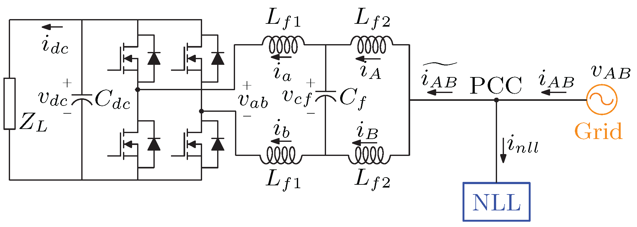
2. LCL-Filter-Based PWM Rectifier
2.1. Parameters and Capabilities
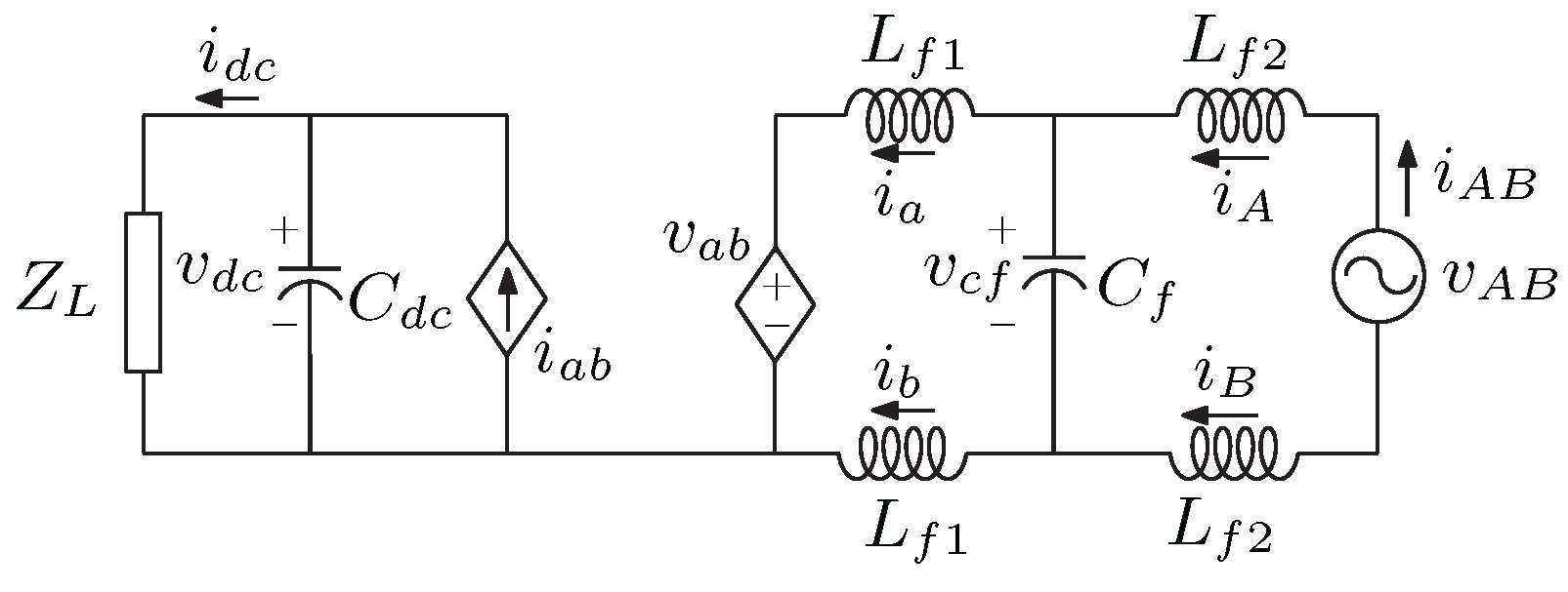
2.2. Modeling
- The PWM rectifier is modeled in the time domain considering the average model. This modeling is justified because the switching frequency is high enough with respect to the grid’s fundamental frequency.
- The components are considered ideal. This consideration is justified because the effect of an integrator that will be introduced into the closed-loop controller has the capability of robustness against constant parameter variations, such as parasitic parameters.
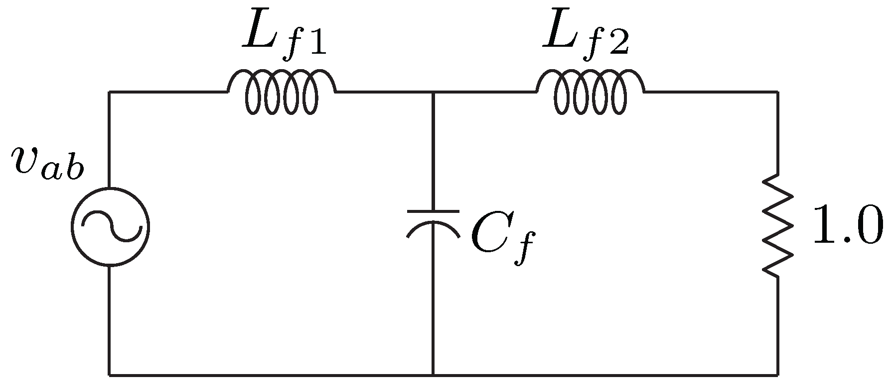
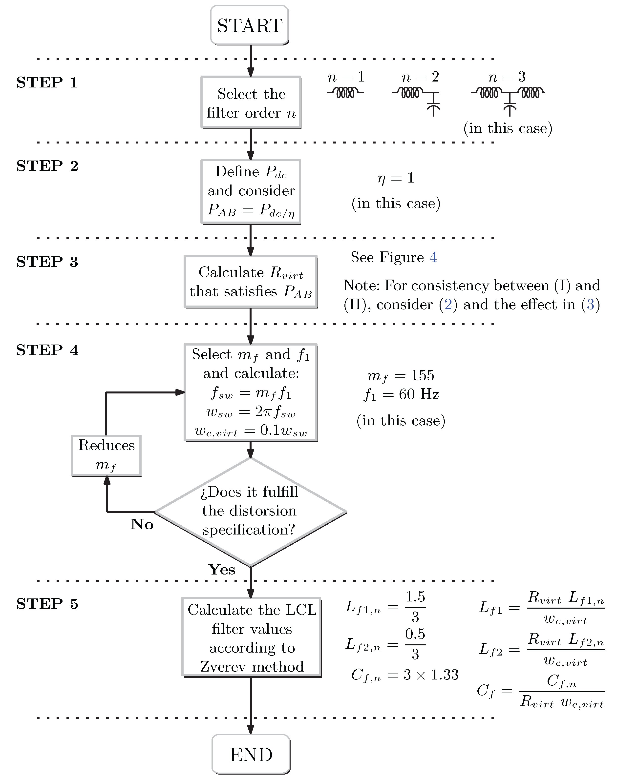
2.3. LCL Filter Design
- 1.
- Select the filter order n. In this case, .
- 2.
- From the power specification of the PWM rectifier on the DC side, consider that the AC power is the same, i.e., . For practical design, can be selected as lower than one.
- 3.
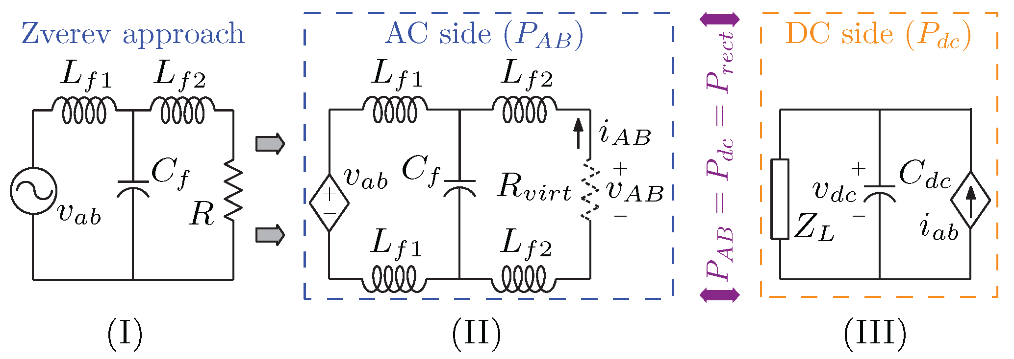
- Calculate a “virtual” resistance , whose value shall represent the AC power needed to cover the DC power requirements, as shown in Figure 4.
- 4.
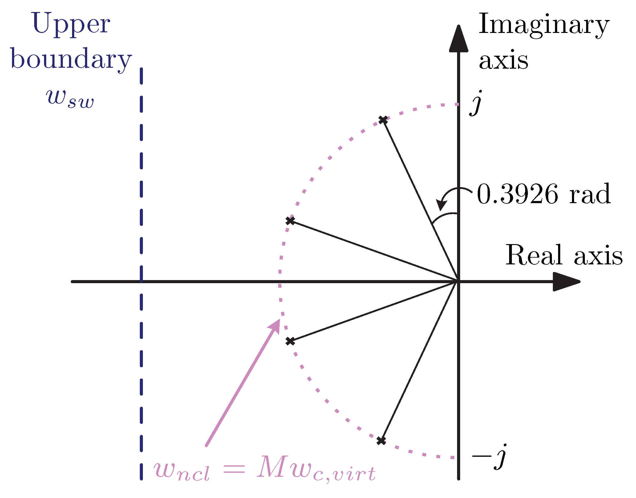
- Select the switching frequency and the cut frequency , where , with the frequency modulation index , the fundamental frequency Hz, and is selected one decade lower than ; thus, . Note that can be obtained for a desired attenuation of the most relevant harmonics of according to the needed specification.
- 5.
- Calculate the values of the LCL filter according to Zverev method [21]: (i) For a third order filter, the normalized values are(ii) Then, denormalizing

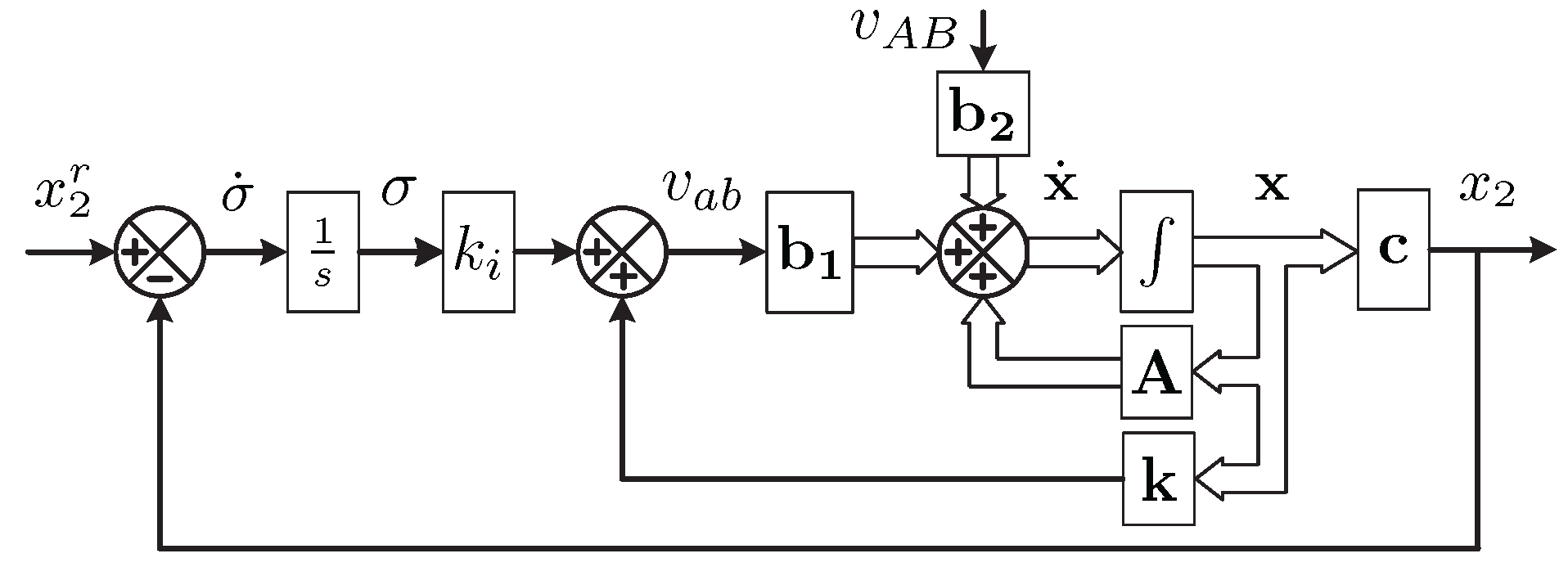
3. Control System Design
- As the LCL filter was designed to cope with the DC power requirements, a linear controller is proposed just for controlling the power flux through the LCL filter.
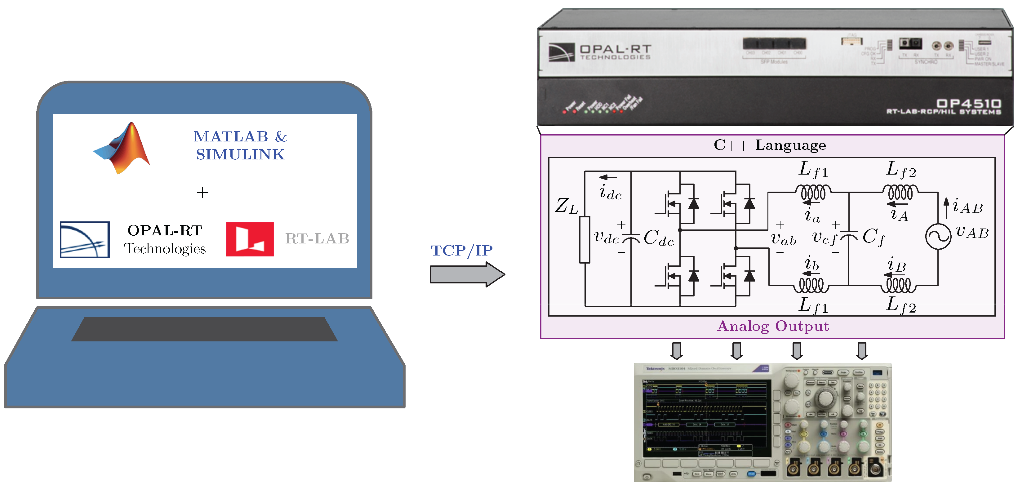
4. Software-in-the-Loop Simulation Results of the PWM Rectifier
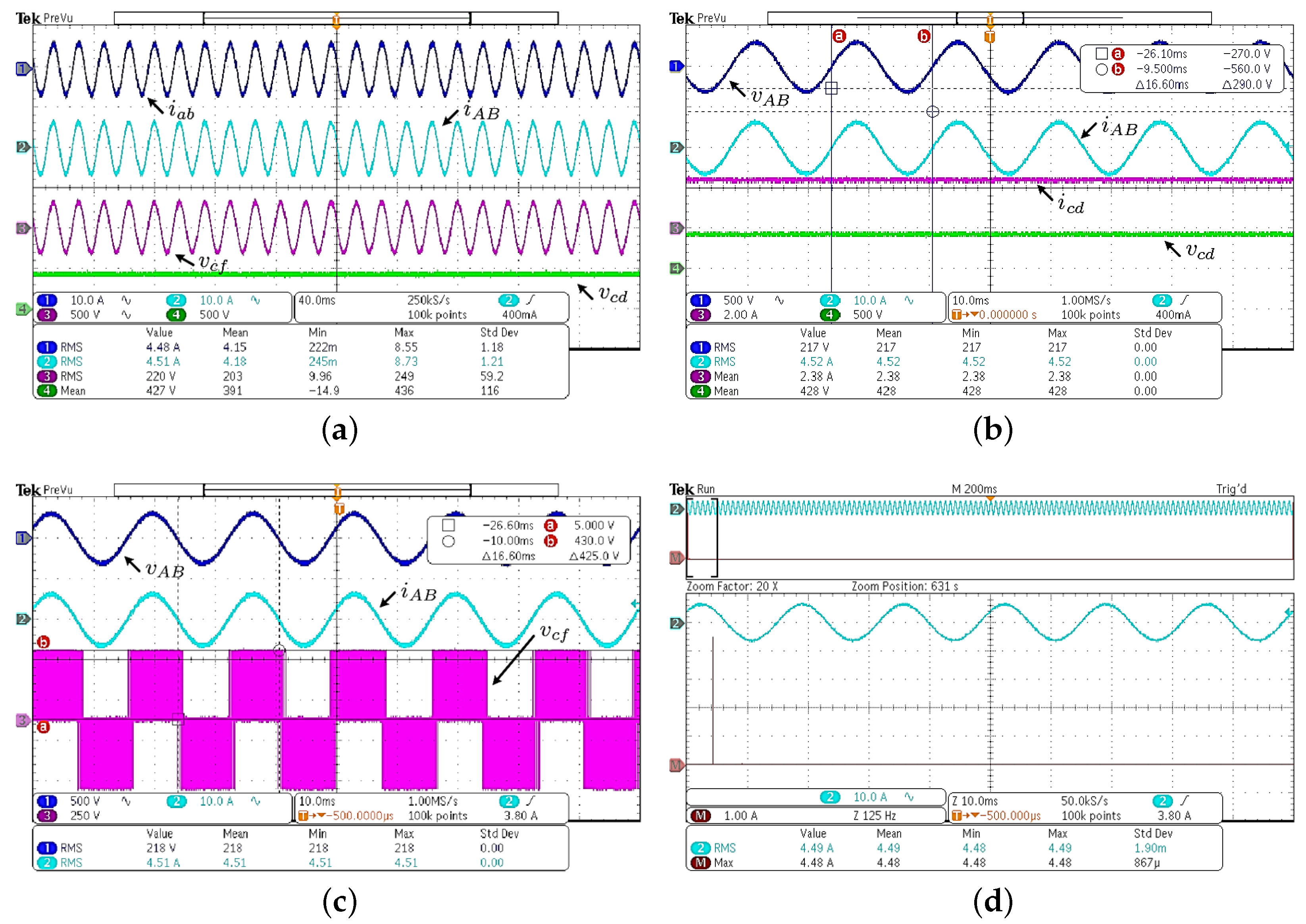
4.1. Steady-State Performance
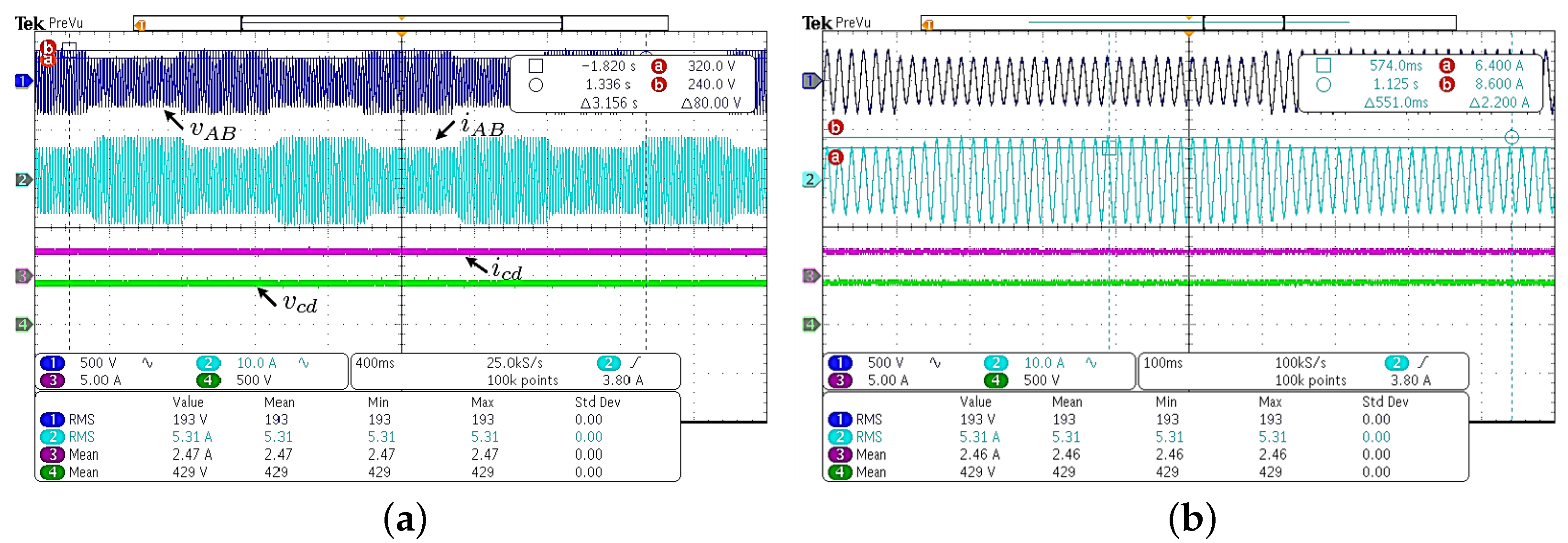
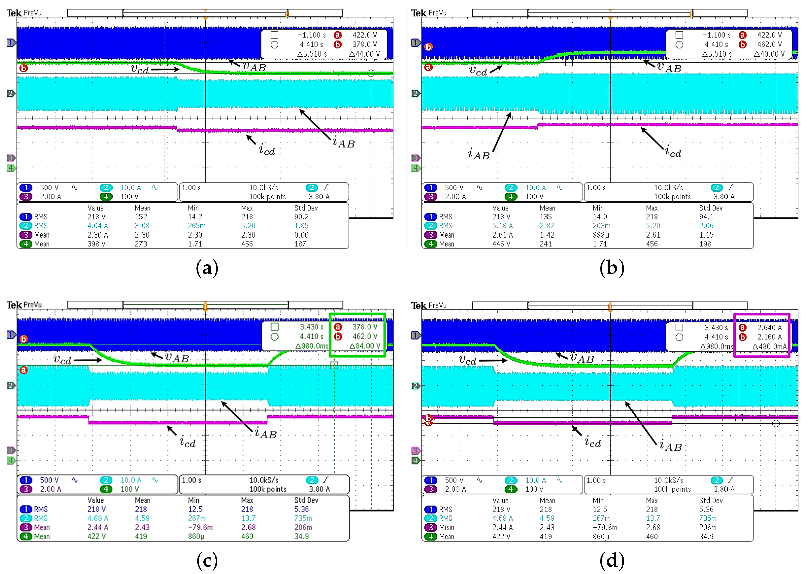
4.2. Grid Voltage Sags without DC Load Variation
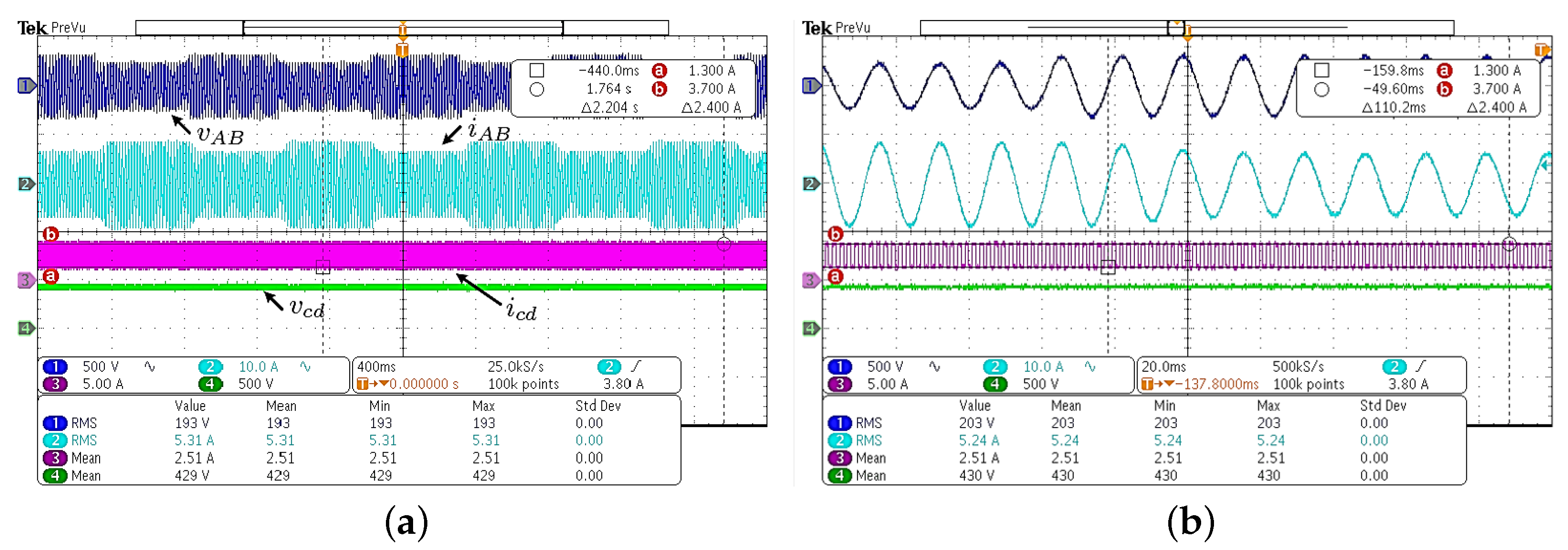
4.3. Grid Voltage Sags and Dynamic DC Load Simultaneously
4.4. DC Voltage Reference Changes
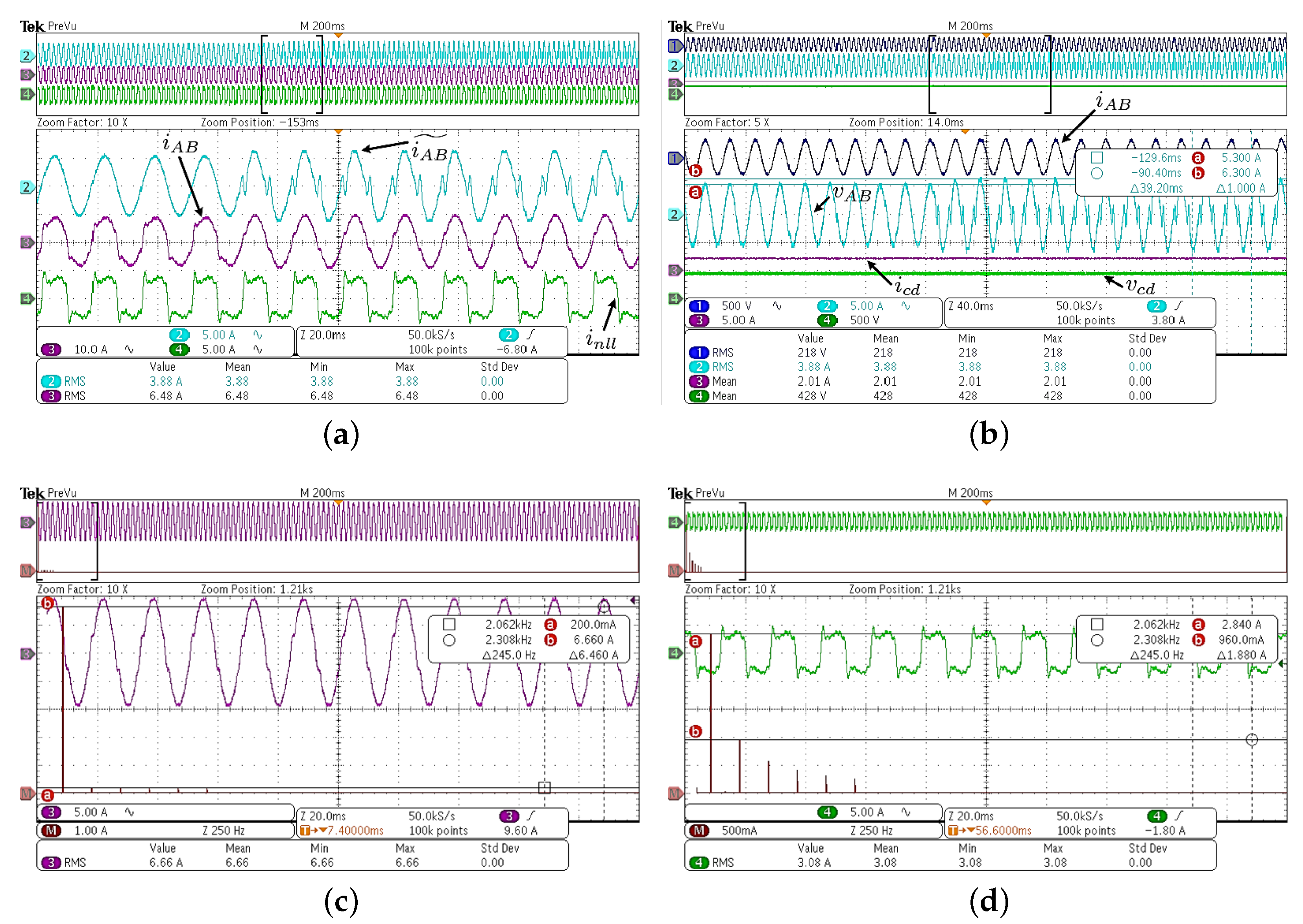
4.5. Harmonic Current Compensation
4.6. Grid Voltage Sags, Dynamic DC Load and Harmonic Current Compensation Simultaneously
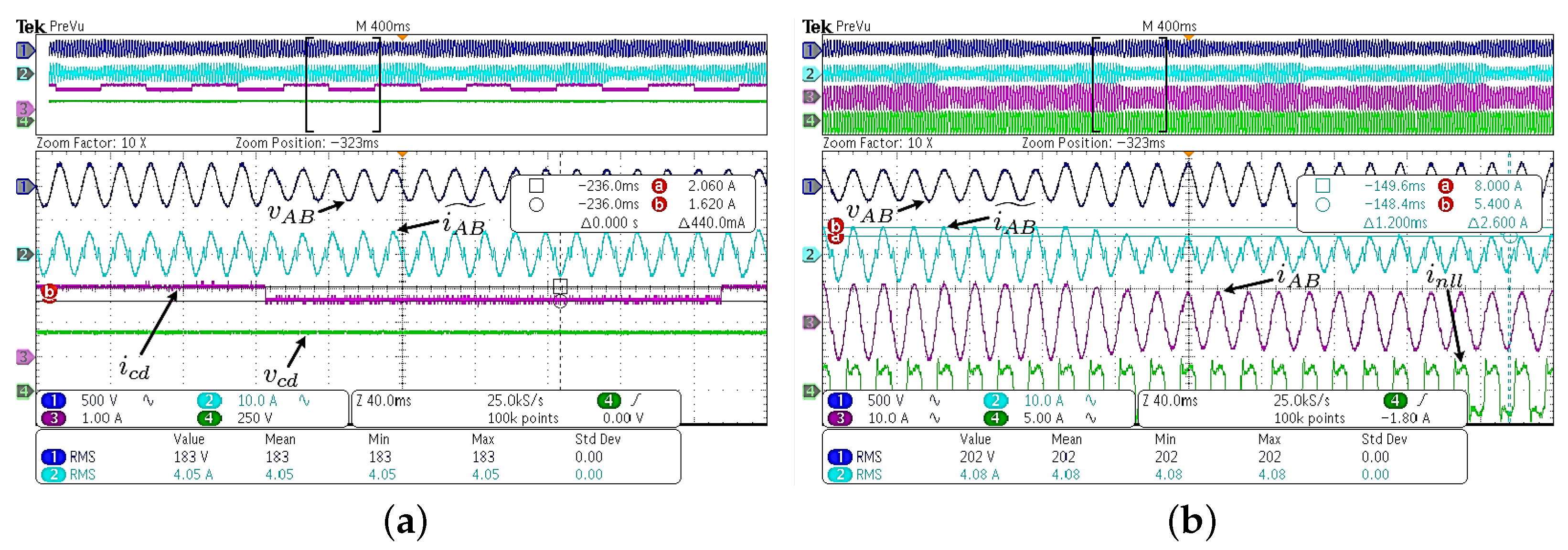
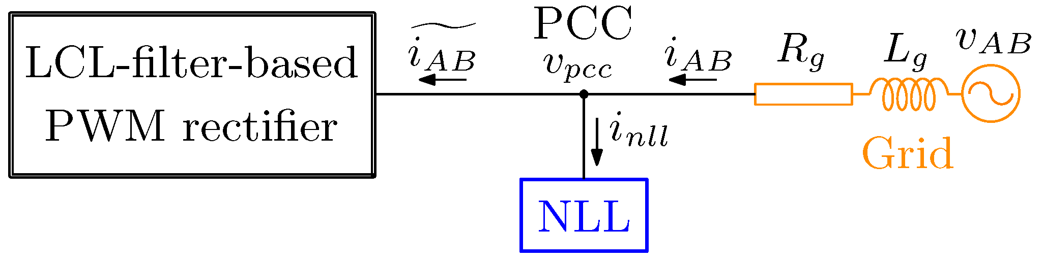
4.7. Grid Voltage Sags, Dynamic DC Load and Harmonic Current Compensation Simultaneously Considering a Grid Impedance
5. Conclusions
Author Contributions
Funding
Conflicts of Interest
References
- Willis, C.H. Applications of Harmonic Commutation for Thyratron Inverters and Rectifiers. Trans. Am. Inst. Electr. Eng. 1933, 52, 701–707. [Google Scholar] [CrossRef]
- Kakkar, S.; Maity, T.; Ahuja, R.K. Power quality improvement of PWM rectifier using VFOC and LCL filter. In Proceedings of the 2017 IEEE International Conference on Power, Control, Signals and Instrumentation Engineering (ICPCSI), Chennai, India, 21–22 September 2017; pp. 1036–1040. [Google Scholar] [CrossRef]
- Deng, J.; Lei, Y.; Kang, J.S.; Yu, M. A Harmonic Current Suppression Method for Single-Phase PWM Rectifier Based on Feedback Linearization. In Proceedings of the International Conference on Power Energy Systems and Applications (ICoPESA), Singapore, 25–27 February 2022; pp. 90–95. [Google Scholar] [CrossRef]
- Vaideeswaran, V.; Veerakumar, S.; Sharmeela, C.; Bharathiraja, M.; Chandrasekaran, P. Modelling of an Electric Vehicle Charging Station with PWM Rectifier to mitigate the Power Quality Issues. In Proceedings of the Transportation Electrification Conference (ITEC-India), New Delhi, India, 16–19 December 2021; pp. 1–6. [Google Scholar] [CrossRef]
- Nunez, C.; Lira, J.; Visairo, N.; Echavarría, R. Analysis of the Boundaries to Compensate Voltage Sag Events Using a Single Phase Multi-Level Rectifier. EPE J. 2010, 20, 5–11. [Google Scholar] [CrossRef]
- Tawfeeq, O.T.; Ibrahim, A.Y.; Alabbawi, A.A.M. Study of a Five-Level PWM Rectifier Fed DC Motor Drive. In Proceedings of the 7th International Conference on Electrical and Electronics Engineering (ICEEE), Antalya, Turkey, 14–16 April 2020; pp. 126–129. [Google Scholar] [CrossRef]
- Changizian, M.; Mizani, A.; Shoulaie, A. A new frequency control method to enhance fault ride-through capability of VSC-HVDC systems supplying industrial plants. Electr. Power Syst. Res. 2023, 214, 108843. [Google Scholar] [CrossRef]
- Yang, J.; Meng, N. Multi-loop power control strategy of current source PWM rectifier. Energy Rep. 2022, 8, 11675–11682. [Google Scholar] [CrossRef]
- Bian, C.; Liu, S.; Xing, H.; Jia, Y. Research on fault-tolerant operation strategy of rectifier of square wave motor in wind power system. CES Trans. Electr. Mach. Syst. 2021, 5, 62–69. [Google Scholar] [CrossRef]
- Lhachimi, H.; El Kouari, Y.; Sayouti, Y. Control strategy of DFIG for wind energy system in the grid connected mode. In Proceedings of the International Renewable and Sustainable Energy Conference (IRSEC), Marrakech, Morocco, 14–17 November 2016; pp. 515–520. [Google Scholar] [CrossRef]
- Narayanan, V.; Kewat, S.; Singh, B. Solar PV-BES Based Microgrid System With Multifunctional VSC. IEEE Trans. Ind. Appl. 2020, 56, 2957–2967. [Google Scholar] [CrossRef]
- Shwetha, G.; Guruswamy, K.P. Performance Analysis of PWM Rectifier as Charger for Electric Vehicle Application. In Proceedings of the International Conference on Integrated Circuits and Communication Systems (ICICACS), Raichur, India, 24–25 February 2023; pp. 1–7. [Google Scholar] [CrossRef]
- Thangavel, S.; Mohanraj, D.; Girijaprasanna, T.; Raju, S.; Dhanamjayulu, C.; Muyeen, S.M. A Comprehensive Review on Electric Vehicle: Battery Management System, Charging Station, Traction Motors. IEEE Access 2023, 11, 20994–21019. [Google Scholar] [CrossRef]
- Wai, R.J.; Yang, Y. Design of Backstepping Direct Power Control for Three-Phase PWM Rectifier. IEEE Trans. Ind. Appl. 2019, 55, 3160–3173. [Google Scholar] [CrossRef]
- Verrelli, C.; Bigarelli, L.; di Benedetto, M.; Lidozzi, A.; Solero, L. A new nonlinear control of an active rectifier for variable speed generating units. Control Eng. Pract. 2023, 139, 105653. [Google Scholar] [CrossRef]
- Application Report: Understanding Boost Power Stages in Switchmode Power Supplies; Technical Report; Texas Instrument: Dallas, TX, USA, 1999.
- Sira-Ramirez, H.; Ortega, R.; Perez-Moreno, R.; Garcia-Esteban, M. A Sliding Controller-Observer for DC-to-DC Power Converters: A Passivity Approach. In Proceedings of the 1995 34th IEEE Conference on Decision and Control, New Orleans, LA, USA, 3–15 December 1995. [Google Scholar] [CrossRef]
- Marzouki, A.; Hamouda, M.; Fnaiech, F. Nonlinear control of three-phase active rectifiers based L and LCL filters. In Proceedings of the International Conference on Electrical Engineering and Software Applications, Hammamet, Tunisia, 23–25 October 2013; pp. 1–5. [Google Scholar] [CrossRef]
- Degioanni, F.; Zurbriggen, I.G.; Ordonez, M. Fast and Reliable Geometric-Based Controller for Three-Phase PWM Rectifiers. In Proceedings of the Applied Power Electronics Conference and Exposition (APEC), New Orleans, LA, USA, 15–19 March 2020; pp. 1891–1896. [Google Scholar] [CrossRef]
- Foti, S.; Scelba, G.; Testa, A.; Sciacca, A. An Averaged-Value Model of an Asymmetrical Hybrid Multi-Level Rectifier. Energies 2019, 12, 589. [Google Scholar] [CrossRef]
- Zverev, A.I. Handbook of Filter Synthesis; John Wiley and Sons, Inc.: Hoboken, NJ, USA, 1967. [Google Scholar]
- Arellanes, A.; Nuñez, C.; Visairo, N.; Valdez-Fernandez, A.A. An Improvement of Holistic Control Tuning for Reducing Energy Consumption in Seamless Transitions for a BESS Grid-Connected Converter. Energies 2022, 15, 7964. [Google Scholar] [CrossRef]
- IEEE Std 1547-2018; IEEE Standard for Interconnection and Interoperability of Distributed Energy Resources with Associated Electric Power Systems Interfaces. IEEE: New York, NY, USA, 2018.
- Esparza, M.; Segundo, J.; Gurrola-Corral, C.; Visairo-Cruz, N.; Barcenas, E.; Barocio, E. Parameter Estimation of a Grid-Connected VSC Using the Extended Harmonic Domain. IEEE Trans. Ind. Electron. 2019, 66, 6044–6054. [Google Scholar] [CrossRef]


| Parameter or Condition | Symbol | Value |
|---|---|---|
| Nominal active power. | 1 kW | |
| Grid voltage. | 220 V | |
| Power factor. | PF | ≈1 |
| Grid current total harmonic distorsion. | THD | ≤5% (at full load) |
| DC bus voltage reference. | 420 V | |
| Grid voltage sag ride-through capability. | yes | |
| Harmonic current compensation capability. | yes | |
| Dynamical DC load and voltage sag ride-through | ||
| capability simultaneously. | yes | |
| DC bus voltage variation capability. | yes | |
| Dynamical DC load, voltage sag ride-through and | ||
| harmonic current compensation simultaneously. | yes |
| Parameter | Symbol | Value |
|---|---|---|
| Nominal active power | 1 kW | |
| Grid voltage | 220 V | |
| DC bus voltage reference | 420 V | |
| Rectifier switching frequency | 9.3 kHz | |
| Grid frequency | , | 60 Hz, 377 rad/s |
| DC-link capacitor | 5000 F | |
| Rectifier side inductance | 4.14 mH | |
| Grid side inductance | 1.38 mH | |
| Capacitor of the LCL filter | 14.14 F | |
| DC equivalent load resistance | 176.4 | |
| Controller gains | , , , | −1.13, −3.57, 0.09, 26,295 |
| Time step | 10 s | |
| Active power of the NLL | 622.22 W (62% ) | |
| THD current of the NLL | THD | 42.88% |
Disclaimer/Publisher’s Note: The statements, opinions and data contained in all publications are solely those of the individual author(s) and contributor(s) and not of MDPI and/or the editor(s). MDPI and/or the editor(s) disclaim responsibility for any injury to people or property resulting from any ideas, methods, instructions or products referred to in the content. |
© 2023 by the authors. Licensee MDPI, Basel, Switzerland. This article is an open access article distributed under the terms and conditions of the Creative Commons Attribution (CC BY) license (https://creativecommons.org/licenses/by/4.0/).
Share and Cite
Viera Díaz, R.I.; Nuñez, C.; Visairo Cruz, N.; Segundo Ramírez, J. A Polynomial Synthesis Approach to Design and Control an LCL-Filter-Based PWM Rectifier with Extended Functions Validated by SIL Simulations. Energies 2023, 16, 7382. https://0-doi-org.brum.beds.ac.uk/10.3390/en16217382
Viera Díaz RI, Nuñez C, Visairo Cruz N, Segundo Ramírez J. A Polynomial Synthesis Approach to Design and Control an LCL-Filter-Based PWM Rectifier with Extended Functions Validated by SIL Simulations. Energies. 2023; 16(21):7382. https://0-doi-org.brum.beds.ac.uk/10.3390/en16217382
Chicago/Turabian StyleViera Díaz, Rosa Iris, Ciro Nuñez, Nancy Visairo Cruz, and Juan Segundo Ramírez. 2023. "A Polynomial Synthesis Approach to Design and Control an LCL-Filter-Based PWM Rectifier with Extended Functions Validated by SIL Simulations" Energies 16, no. 21: 7382. https://0-doi-org.brum.beds.ac.uk/10.3390/en16217382