
Numerical Modeling of Two-Phase Flow inside a Wet Flue Gas Absorber Sump

Faculty of Mechanical Engineering, University of Maribor, 2000 Maribor, Slovenia
*
Author to whom correspondence should be addressed.
†
These authors contributed equally to this work.
Energies 2023, 16(24), 8123; https://0-doi-org.brum.beds.ac.uk/10.3390/en16248123
Submission received: 24 November 2023
/
Revised: 11 December 2023
/
Accepted: 14 December 2023
/
Published: 18 December 2023
(This article belongs to the Topic Fluid Mechanics)
Abstract
:A numerical model of a flue gas scrubber sump is developed with the aim of enabling optimization of the design of the sump in order to reduce energy consumption. In this model, the multiphase flow of the continuous phase, i.e., water, and the dispersed phase, i.e., air bubbles, is considered. The air that is blown in front of the agitators, as well as the influence of the flow field of the agitators on the distribution of the dispersed phase and the recirculation pumps as outlet, is modeled. The bubble Sauter mean diameter is modeled using the population balance model. The model is used to analyze operating parameters such as the bubble retention time, the average air volume fraction, bubble Sauter mean diameter, the local distribution of the bubble size and the amount of air escaping from the pump outlets at two operating points. The purpose of the model is to simulate the two-phase flow in the sump of the flue gas scrubber using air dispersion technology with a combination of spargers and agitators, which, when optimized, reduces energy consumption by 33%. The results show that the homogeneity of air is lower in the bottom part of the absorber sump and that the amount of air escaping through recirculation pipes equals 1.2% of the total air blown into the absorber sump. The escaping air consists mainly of bubbles smaller than 6 mm. Additional operating point results show that halving the magnitude of the linear momentum source lowers the air retention, as well as the average homogeneity of the dispersed air.
1. Introduction
Flue gas desulfurization methods with the aim of reducing the impact on human health have been known since the early days [1]. The first ideas relating to the removal of sulfur dioxide (SO2) from flue gases emerged in England around 1850, where the consequences of the industrial revolution began to manifest themselves not only as economic indicators but also as a serious threat to human health.
Throughout history, numerous flue gas desulfurization technologies have been developed [2,3], primarily aimed at cleaning emissions from coal-fired power plants and metallurgical plants. It was found that certain additives in water improve the ability to remove SO2 from flue gases. The first studies were carried out on the solubility of SO2 in a solution of water and lime, which showed improved properties in terms of flue gas cleaning. Nowadays, most modern flue gas desulfurization plants are based on the wet limestone process [4]. The reason for this is that limestone is abundant in nature and can be processed cost-effectively for use in FGD plants.
The first larger FGD plants were built in England in the early 20th century. At the beginning, the technology was based on the spraying of water from the river Thames into the flue gas counter flow. The effluent, which contained absorbed SO2, was channeled back into the Thames and posed a significant threat to the river’s ecosystem. Later improvements included the addition of lime to the river water before spraying, which increased the alkalinity of the water and, thus, the proportion of neutral CaSO3 in the wastewater. This measure improved the problem of acidic emissions into the Thames. Another improvement concerned the modification of the scrubber itself. A sump was built below the flue gas inlet of the absorber, in which the wastewater was retained. The purpose of the absorber sump was to extend the retention time of the wastewater so that more time was available for the reaction of SO2 to form CaSO3. Finally, interest arose in converting CaSO3 into a usable form and in dewatering the obtained byproduct for sale on the market. The proposed method involved the oxidation of CaSO3 into CaSO4·H2O, also known as gypsum. This conversion only partially compensates for the high operating costs of FGD plants, as the gypsum produced as a byproduct is not necessarily of high quality [5] and can rarely be used as a load-bearing material [6]. Additional treatment can improve the mechanical properties of byproduct gypsum [7,8].
There is little literature on the numerical modeling of a real FGD absorber sump, as the numerical modeling of flue gas scrubbers mainly focuses on the optimization of the absorption process of SO2 from flue gases into liquid droplets. Arif et al. [9] conducted a Euler–Lagrangian analysis of FGD absorbers using Lagrangian tracking of droplets generated on absorber spray levels. They concluded that the inlet flue gas velocity distribution has a major influence on the efficiency of the FGD absorber. A similar approach was adopted by Marocco et al. [10], who modeled the absorption of SO2 from flue gas into liquid droplets using two-film theory. They reported good agreement with the experimental results in terms of flue gas temperature measurements, absorber pressure drop and the overall efficiency of SO2 removal. Qu et al. [11,12] investigated the effects of different droplet diameters, as well as spray injections and spray morphologies, on the efficiency of FGD absorbers. Flue gas scrubbing strongly depends on the droplet diameter, as larger droplets reduce the absorption rate of SO2, and smaller droplets evaporate faster preventing absorption.
Regarding the modeling of the absorber sump, the aim of numerical modeling is to optimize the air dispersion using different combinations of spargers and agitators (mixers) [13], which can be included in a dynamic model of an FGD plant [14]. Gomez et al. [15] created a detailed numerical model of an FGD plant using the Euler–Euler approach, which includes both the scrubber section and the absorber sump. By implementing chemical kinetics, including gypsum formation models, they gained detailed insights into actual limestone consumption. The latter is also dependent on the actual limestone dissolution rate [16]. To model the effects of agitators on air dispersion in different aeration systems, either direct modeling with the MRF approach is used or the agitator flow field is modeled as a linear momentum source [17].
The capability of numerical modeling of process plants has been strongly influenced throughout history by the development of multiphase flow modeling and available hardware. For a thorough description of all chemical and physical phenomena inside the FGD absorber and the absorber sump, especially with regard to the modeling of SO2 absorption, O2 absorption, droplet drying, etc., advanced CFD approaches must be used [18,19,20].
Society has been confronted with exponential growth in production capacities for decades. In order to satisfy all needs, energy production must follow suit, which is not possible without ecological consequences. Today, these consequences can be divided into an increase in the concentration of carbon dioxide in the atmosphere—a direct consequence of the use of fossil fuels—and the rapid depletion of natural resources—a direct consequence of consumerism. It seems that the environmental measures taken by industrialized countries are primarily aimed at the former. Decision makers see the solution primarily in reducing the use of fossil fuels and replacing them with renewable sources.
One of the consequences of these measures is increasing globalization, which is pushing industrialized countries into greater dependence on countries that are rich in natural resources needed for the transition to renewable energy sources. One example of this is the solarization of the power system based on photovoltaics, which has led to an increased demand for silicon-based semiconductor materials, most of which are produced in China. European countries are forced by their own regulations to rely on developing countries, which strengthens their competitiveness in the global market.
Current environmental policy, particularly in relation to greenhouse gas emissions, has not yet shown the improvements for which it was designed. This is partly due to the lack of global consensus and partly due to the interests of countries and companies whose success is based on maximizing consumption and, therefore, production. At this point, it becomes clear why environmental regulations are predominantly focused in one direction. Any measure to drastically reduce consumption can have disastrous consequences for a modern country in today’s economic system, as the general indicator of a country’s prosperity is expressed in the buying power of the population and, consequently, in production growth. The fact remains that we only have a finite supply of natural resources and that it is crucial for a sustainable existence to utilize them properly.
Due to these concerns, we developed a numerical model of an FGD absorber sump with the aim of improving the energy consumption characteristics of FGD systems.
2. Flue Gas Scrubbing
2.1. Physical Background
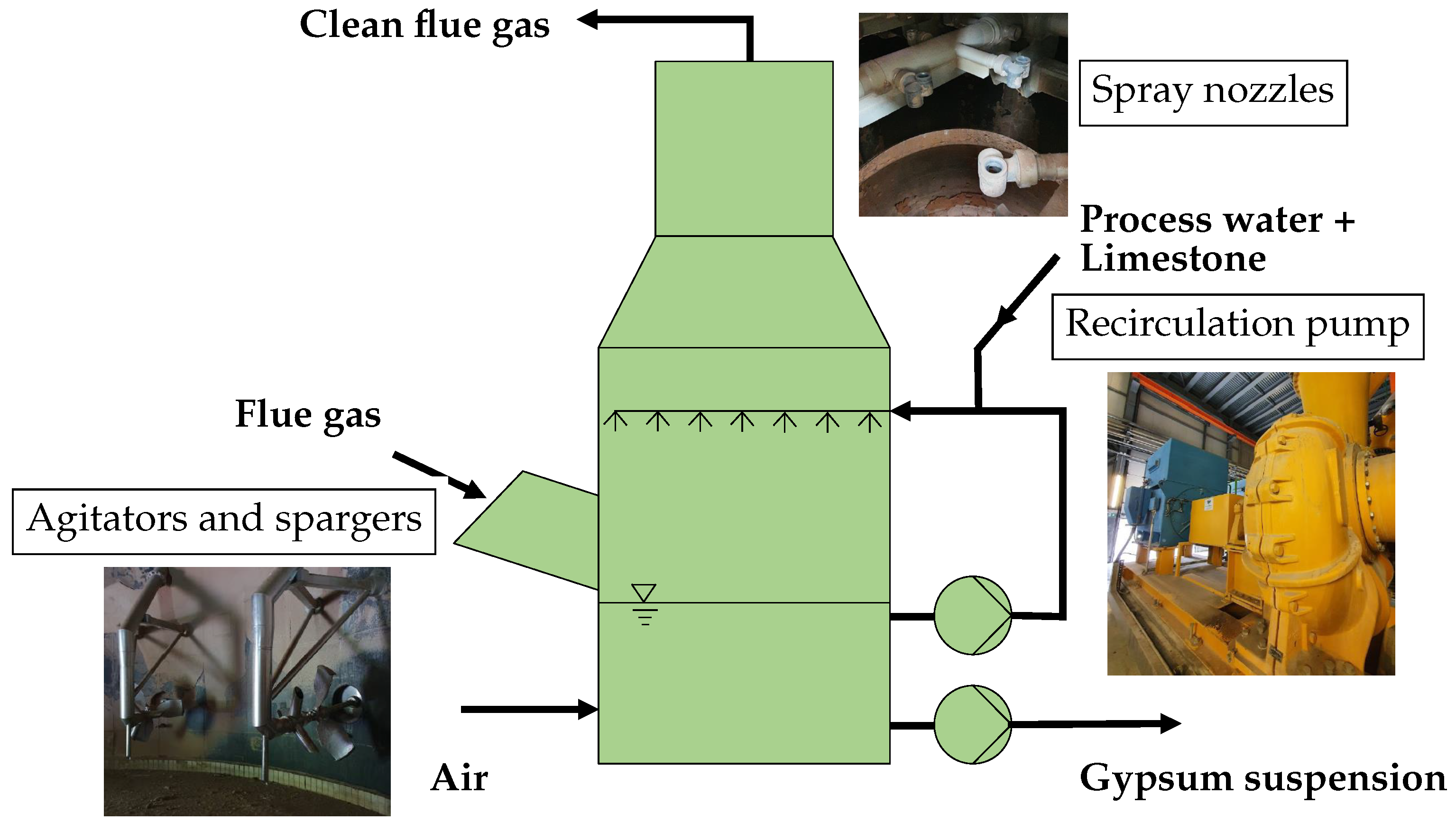
The desulfurization of flue gases from a thermal power plant is carried out using the wet calcite process to clean the flue gases of SO2, which is a byproduct of the combustion of sulfur-containing coal [21]. The technology shown in Figure 1 requires the construction of a process building called a flue gas scrubber. Its main objective is to absorb SO2 into liquid droplets that are sprayed into the flue gas counter current as it flows towards the top of the scrubber, into the stack. The droplets are generated on the spray levels in the upper part of the absorber. The liquid consists of water and dissolved limestone, which binds SO2 and produces CaSO3. Droplets of absorbed SO2 fall to the bottom of the absorber, into the absorber sump. The main task of the absorber sump is to maintain the conditions for the formation of a stable product. This is achieved by the further oxidation of CaSO3 to CaSO4 (gypsum), which forms crystals when supersaturated in water. The resulting suspension is circulated from the sump to the spray levels by the so-called recirculation pumps. Oxidation takes place by blowing air directly into the absorber sump. The aim is to achieve a homogeneous distribution of air in the absorber sump with the smallest possible mean bubble diameter in order to maximize the transfer of oxygen from the bubbles into the surrounding liquid. The numerical model of the absorber sump presented here is based on technology that requires the use of a combination of air spargers and agitators to ensure a homogeneous distribution of air bubbles in the absorber sump.
2.2. Scrubber (Absorber) Design
The flue gas enters from the side and is then diverted to the outlet at the top of the scrubber. Next to the FGD absorber, there is normally a separate building housing the recirculation pumps. The diameter of the recirculation pipe must be dimensioned so that the minimum required suspension velocity is achieved to prevent gypsum or limestone particles from settling. A mist eliminator must be installed in the upper part of the absorber to prevent additional process water loss.
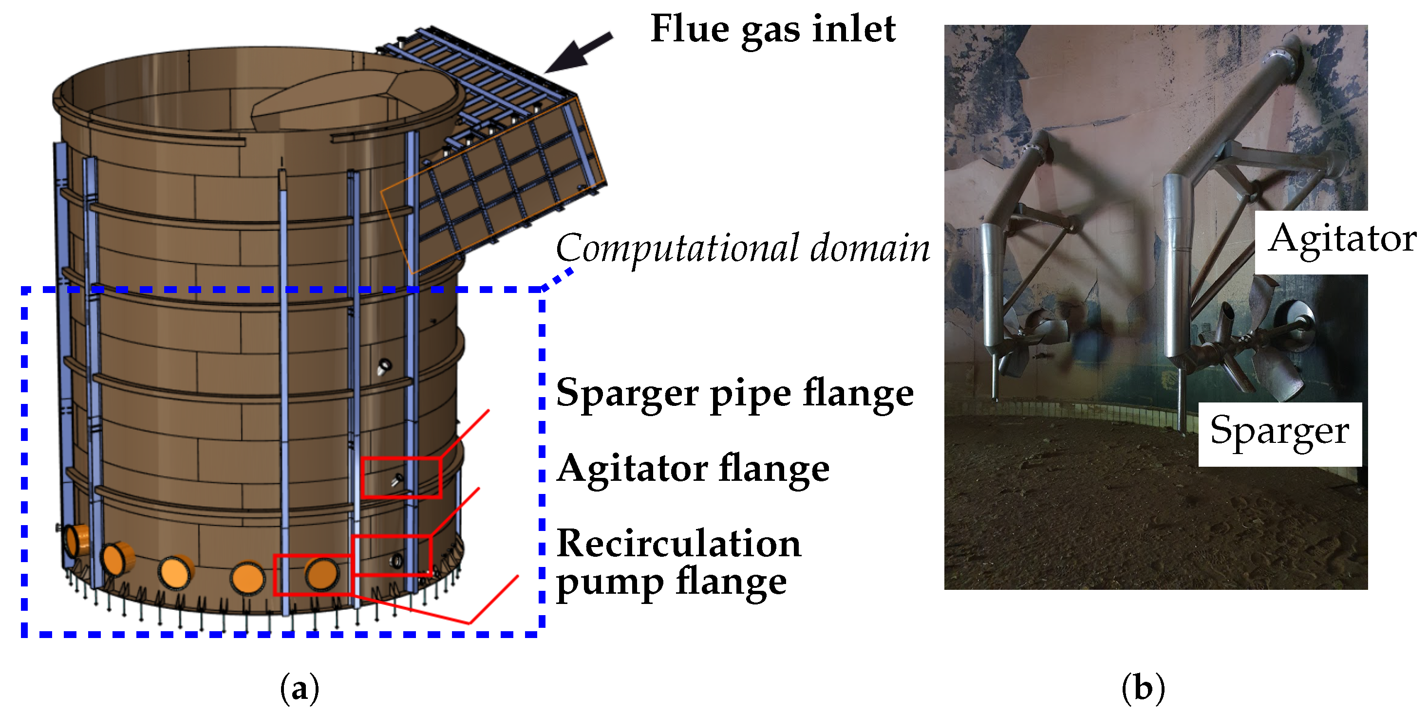
Figure 2a shows the CAD model of the considered FGD absorber. The absorber sump has the following tasks:
- The air dispersion required for the forced oxidation of CaSO3 is achieved by a combination of agitators and air spargers. An example of agitators with corresponding air spargers in a reference project at the Trbovlje Thermal Power Plant (TET) (Slovenia) is shown in Figure 2b. The design of the sump in TET is different from the design we investigated in this study. Instead of a single sparger on the agitator, air is blown into three points in front of the agitator, as shown in the figure.
- The suspension of gypsum and limestone particles to prevent them from settling, thus eliminating the risk of a solid layer forming at the bottom of the absorber sump. The appropriate suspension conditions also create a suitable environment for the growth of gypsum crystals when supersaturation is reached.
- Ensuring volume and, thus, sufficient time for chemical reactions and the absorption of oxygen into the surrounding liquid.
3. Methods
3.1. Governing Equations
Open-source software OpenFoam version 11 [22] was used to simulate the multiphase flow in the absorber sump. The URANS approach was adopted to model the unsteady, turbulent, two-phase flow of the continuous and dispersed phases. The compressible continuity equation for an arbitrary phase () is expressed as
and the compressible momentum equation is expressed as
The governing equations are connected by volume fraction
for phase in cell i. In Equations (2) and (3), is the density, is the velocity vector, p is the pressure and is the vector of the gravitational constant. The term represents all additional momentum sources for the phase. The additional local momentum source is represented by the agitator. The term covers the momentum transfer between the phases and requires the modeling of the forces acting on a bubble. The term is the divergence of the stress tensor, where the latter is defined for compressible fluids as
In Equation (4), is the deformation tensor, which is defined as
For turbulence modeling purposes, the k-Omega SST Sato [23] and k-Epsilon [24] turbulence models were used for the continuous and dispersed phases, respectively.
The population of bubbles in the absorber sump is polydisperse. The reason for the varying size is bubble breakup in areas with high shear flow (agitator area) and coalescence in areas with low shear flow (in the upper part of the absorber sump). The development of the bubble size is described by the population balance model [25] as
where is the number concentration of bubbles in size group j, and is the velocity vector of the dispersed phase. Breakup and coalescence are modeled by the term as the source/sink of the bubbles in size group j. The proportion of the individual size groups is given by
where is the volume fraction of air bubbles that correspond to size group j so that and always holds for n size groups.
3.2. Boundary Conditions
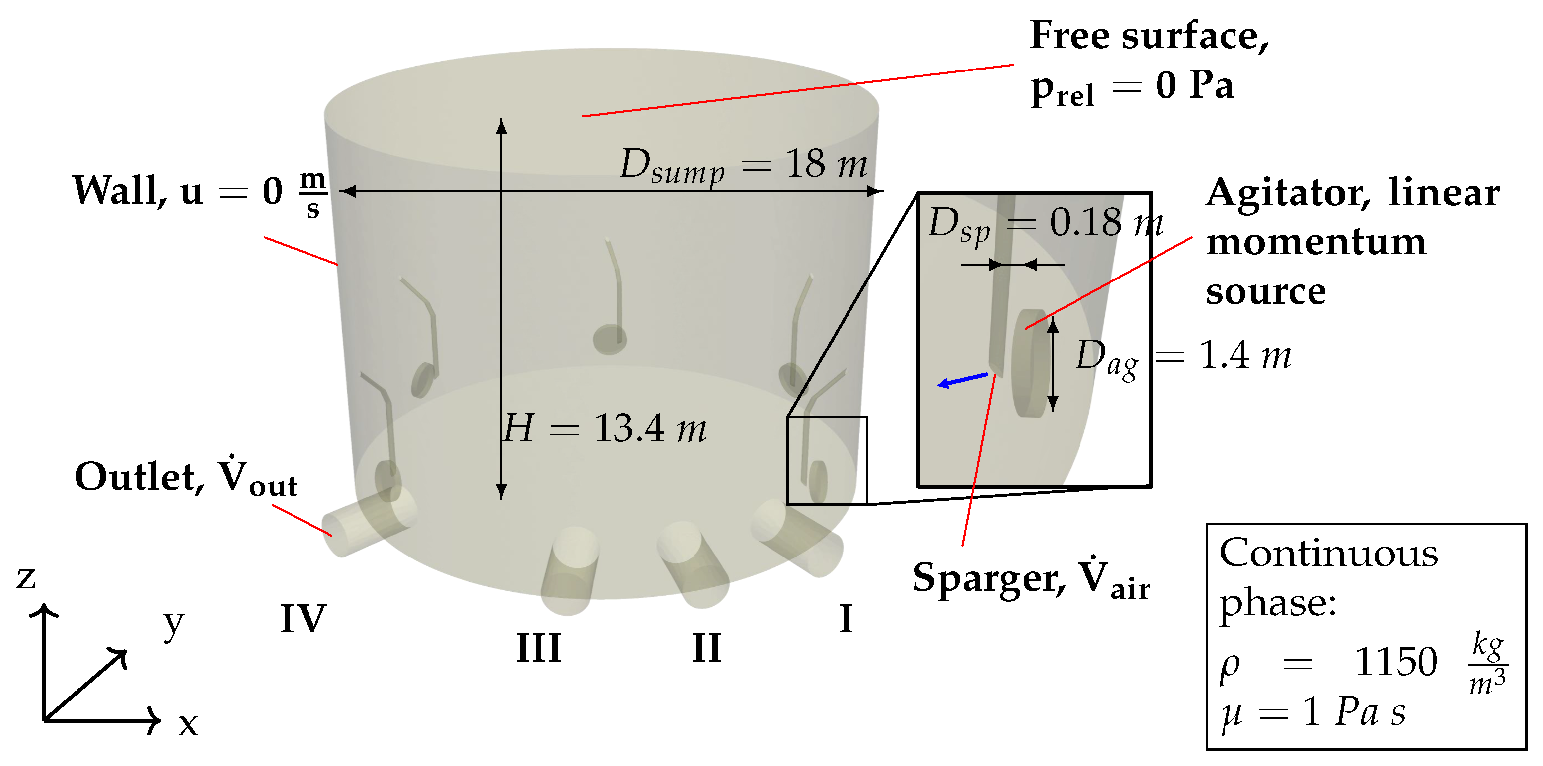
The geometry of the numerical model of the FGD absorber sump is shown in Figure 3. The boundary conditions on the free surface are relatively complex. There, a mixed boundary condition must be defined for the velocity of the continuous phase so that inflow is allowed and outflow is not allowed. For velocity components that are tangential to the free surface (, ), a free slip condition must be employed:
A no-slip boundary condition for the velocity and a Neumann boundary condition with zero gradient for the pressure are defined at the wall. Wall functions are used for turbulent variables, as the mesh size in the region close to the wall fulfills .
The air enters the computational domain through a sparger. A fixed volume fraction of the air and a fixed value for the turbulent variables are defined. The direction of the air inlet is marked with a blue arrow.
In the present numerical model, the agitators are modeled as a linear momentum source. The momentum source is calculated based on the agitator flange axial force, which is provided by the agitator manufacturer as
where denotes the volume taken by the rotating agitator blades.
The key simplifications of the absorber sump for numerical modeling are summarized as follows:
- A mixed boundary condition that enables the inflow of the continuous phase and the outflow of the dispersed phase is applied on the free surface. Since free surface modeling was outside the scope of this research, the applied simplification was allowed.
- The influence of the agitators on the flow field inside of the absorber sump is modeled as a local linear momentum source, since obtaining the exact geometry of the agitator blades can be challenging. The applied linear momentum source was calculated based on the agitator flange axial force provided by the agitator manufacturer.
- The geometry was simplified so that measurement equipment inside of the absorber sump was omitted from the geometry creation.
3.3. Submodels
To model the interaction between the continuous and dispersed phases, we included the following submodels, as available in the OpenFoam CFD package [26]. The forces are accounted for in the momentum equation (Equation (3)) as the sum of the below forces per unit volume as , where q represents the type of force submodel, as presented below.
Drag force between air bubbles and liquid inside of the absorber sump is calculated as
where subscripts d and c represent the dispersed and continuous phases, respectively; is the local bubble diameter; and is drag coefficient, which is calculated as
Shear induced lift force acts on a particle traveling with a relative velocity in a shear flow field of viscous fluid and is calculated as
where is the lift coefficient calculated using the model proposed by Tomiyama et al. [27].
Turbulent dispersion force is modeled as proposed by Burns et al. [28]:
where is the turbulent viscosity of the continuous phase, is the drag coefficient given in Equation (11) and is the turbulent Schmidt number.
Virtual mass force is applicable when one phase accelerates through the surrounding phase. The force is calculated as
where is a virtual mass coefficient and equals . In Equation (14), D denotes the total derivative.
Wall lubrication force occurs when the dispersed phase flows along a wall. The force vector points in a direction normal to the wall. It is calculated as
where denotes the magnitude of the relative velocity of phases tangential to the wall (or ), and is the wall-normal vector. is the wall lubrication force coefficient and is calculated as proposed by Antal et al. [29].
4. Results
4.1. Validation
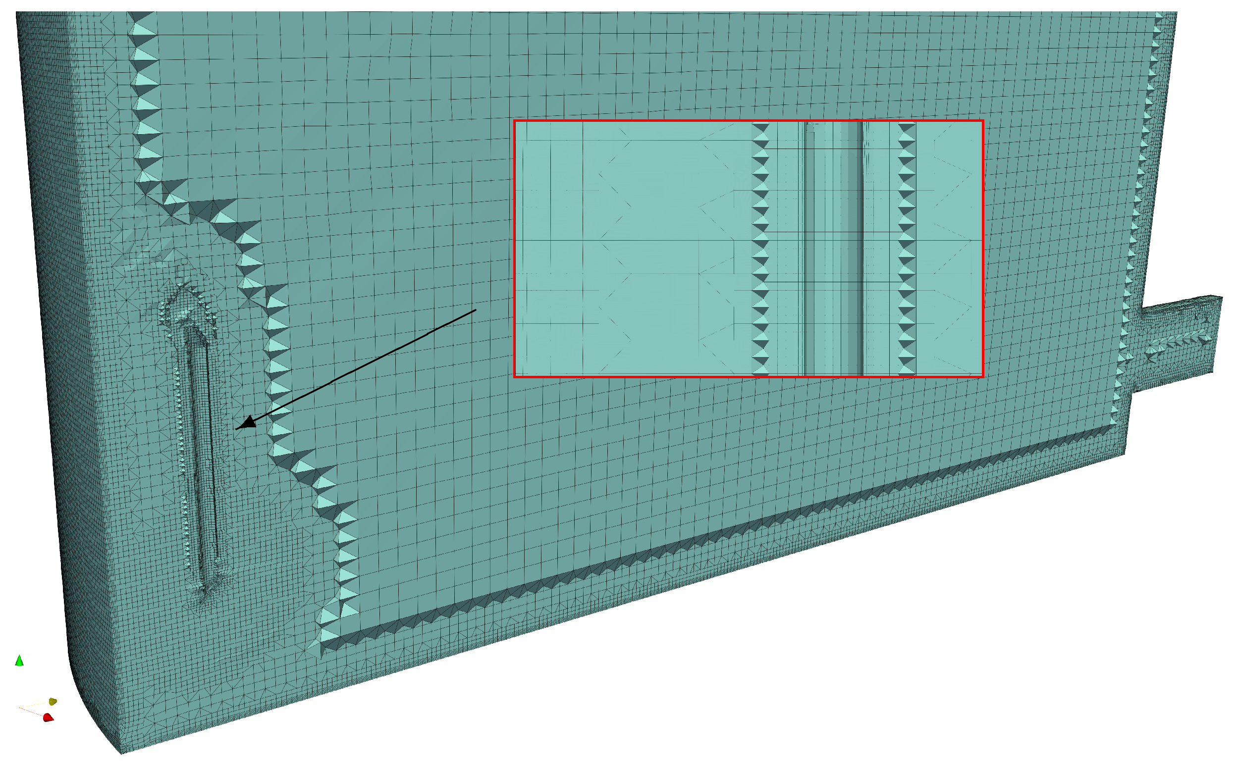
For the numerical modeling of an FGD absorber sump, a mesh with hexagonal elements was created, as shown in Figure 4.
A refinement region was created in the sparger and agitator area, as well as the pump outlet area. Wall element thickness was set to 10 mm.
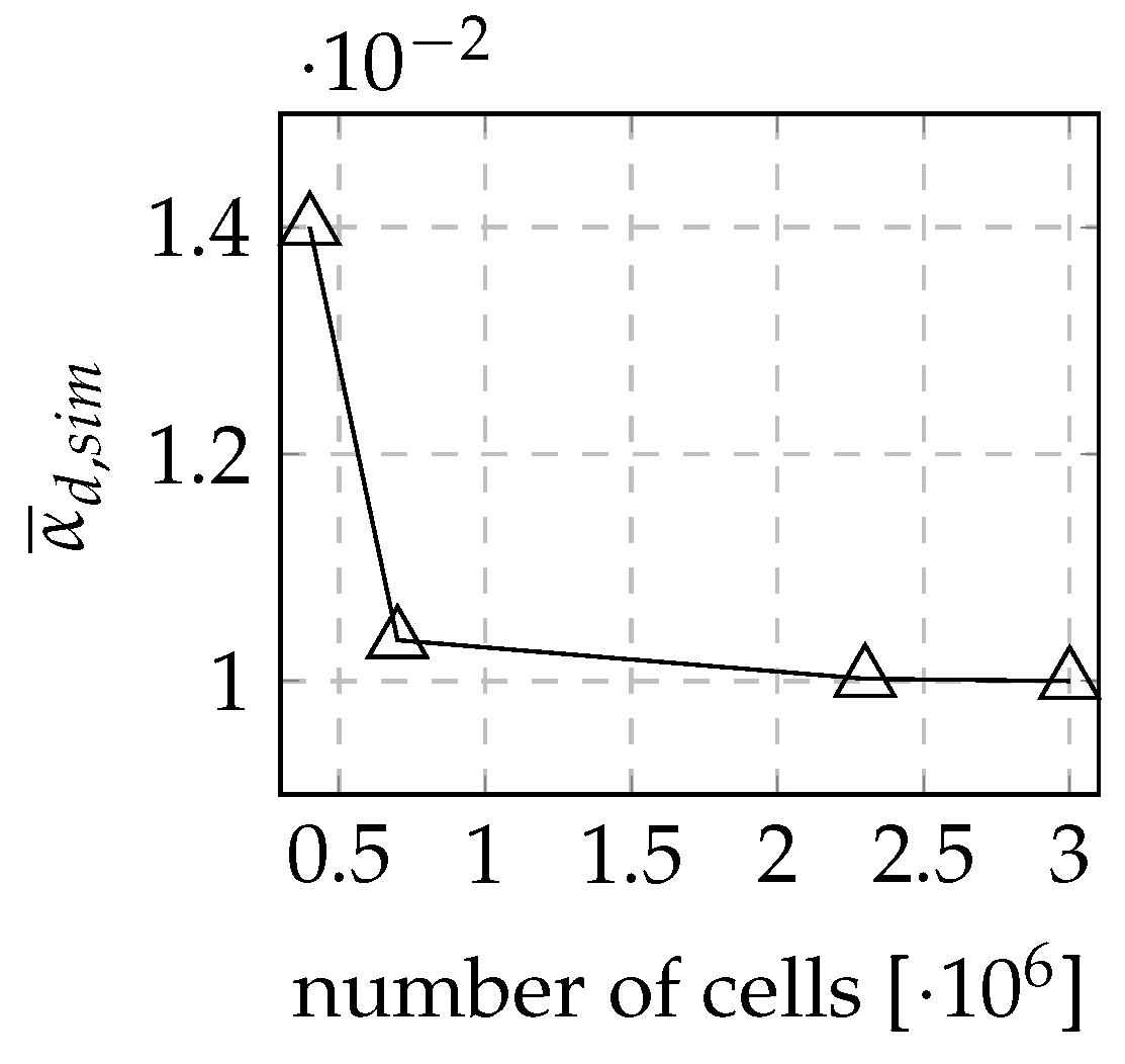
A mesh independence study was conducted to validate the numerical model. Homogeneity profiles and the bulk air volume fraction were compared for four meshes (, , and cells) with varying element sizes. For the unsteady simulation, we set the maximum Courant number to be equal to 1, and the time step was calculated accordingly. First-order numerical schemes were used for both temporal and spatial discretization. The bulk air volume fraction, which is, from the engineering standpoint, the most important parameter, with respect to the number of cells in a mesh is shown in Figure 5. We observed clear convergence of the results, since the results do not significantly change between the 2.3 and 3 million meshes.
Homogeneity of air dispersion was also compared for all meshes. We evaluated the homogeneity based on variance [1], calculated as
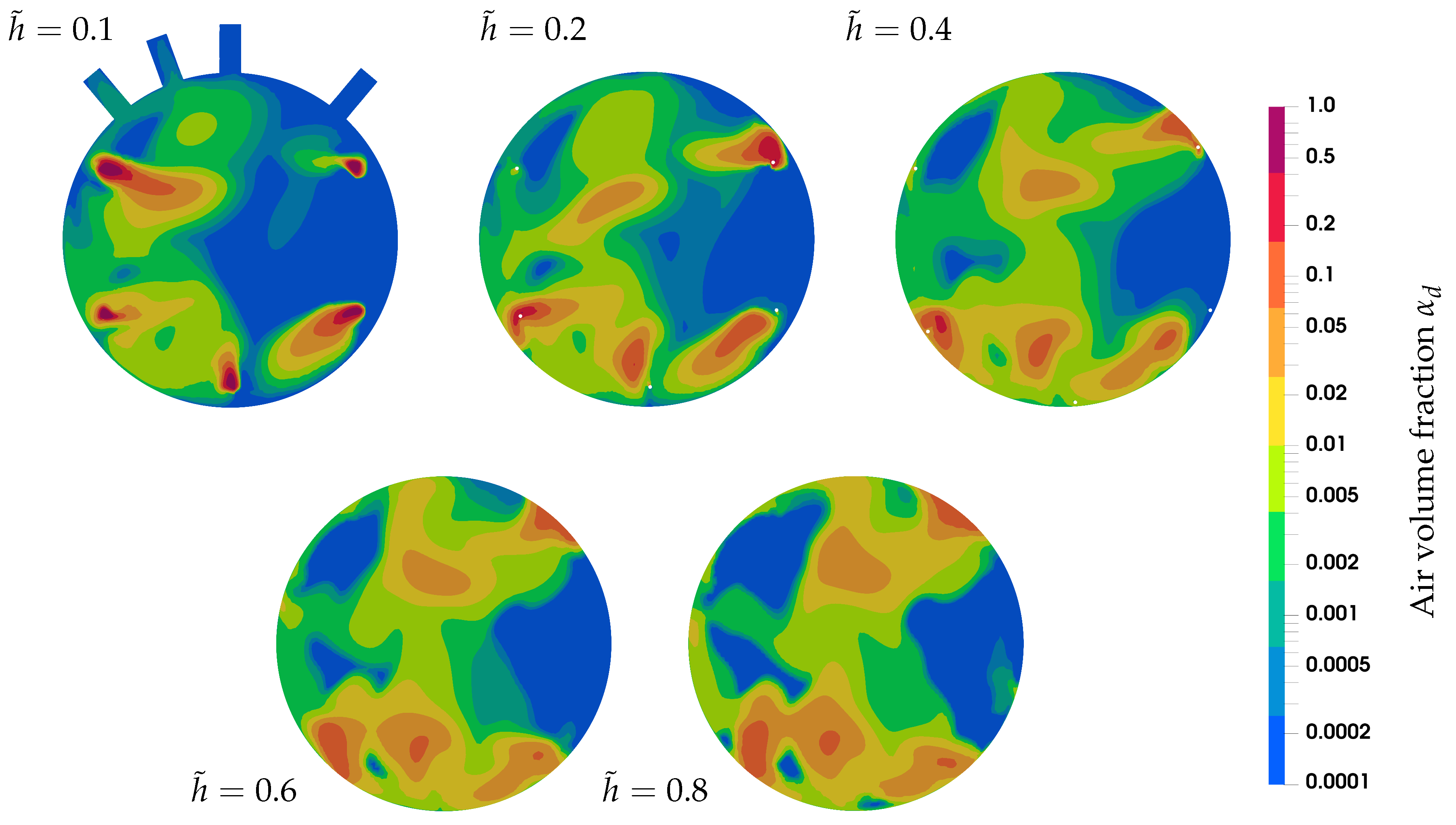
where is the surface area of a cross-sectional plane at a non-dimensional height of absorber sump . Figure 6a shows that the homogeneity is lower in the bottom part of the absorber sump, where air spargers are located. This is expected, since near the sparger inlets, the air bubbles are not yet dispersed properly.
In the lower part of the absorber sump, there is a greater discrepancy in terms of homogeneity between meshes. This can be attributed to a higher gradient of all quantities in this area, as shown in Figure 6b. The gradient of the air volume fraction along the height of the absorber sump was taken as the average gradient along profiles (inset of Figure 6b). The mesh independence study showed satisfactory results, so all subsequent calculations were carried out with the cell mesh.
4.2. Simulation Results
The results were visualized using open-source ParaView 5.10 software. The parameters of the simulation, such as the air inflow (), were selected in accordance with the relative air–CaSO3 ratio (). This parameter means that the total amount of air blown into the absorber sump is of the air required under stoichiometric conditions for the oxidation of the total produced CaSO3.
The simulation showed that the bulk volume fraction of dispersed air in the absorber sump is equal to . Using , we can determine the average retention time of air in the sump with the volume () and the air inflow ().
The distribution of air at different heights in the absorber sump is shown in Figure 7. We can observe the air plume at the inlets of the spargers at and the merging of the plumes towards the upper parts of the absorber sump. We also observe a higher air volume fraction at the first recirculation pump on the left side, indicating a higher escape rate of air through the recirculation pump.
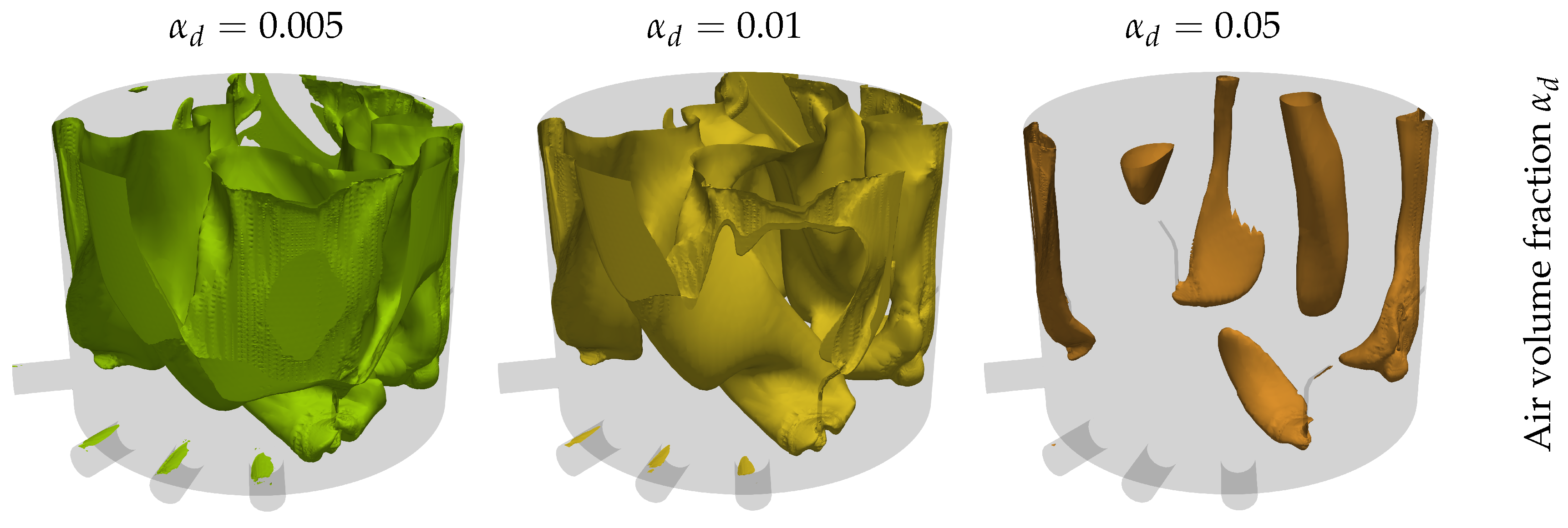
The 3D contours of the air volume fraction are shown in Figure 8. The escape of the air is also visible here. This phenomenon should be avoided, since the escaped air has a significantly lower retention time than the air moving through the absorber sump. The 3D representation shows the bulk movement of the air.
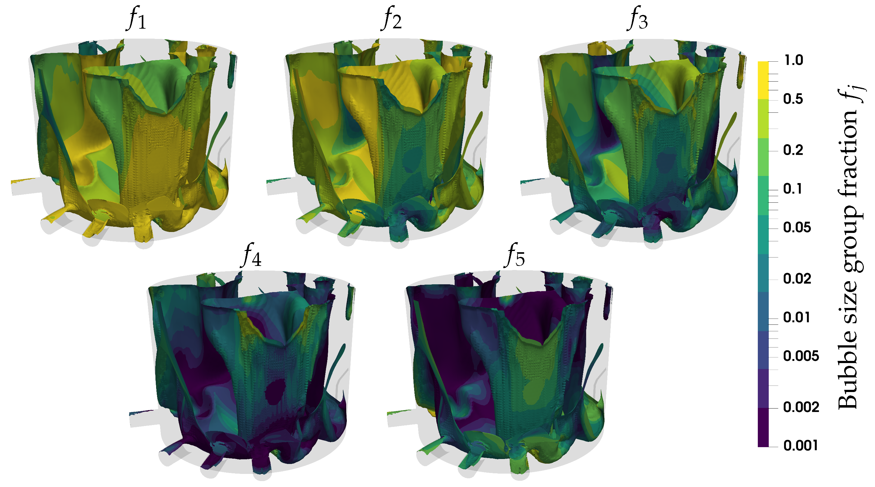
The population balance model allows us to analyze the local size of the bubbles in the absorber sump. The size groups are distributed as shown in Table 1.
The maximum size of the bubbles (size group 5) was determined by the size of the internal diameter of the air sparger. The minimum size (size group 1) was determined empirically by taking the critical Weber number [1] as
where d is the agitator diameter, r is the rotation speed and is the surface tension. The intermediate sizes are distributed in the lower part of the bubble size spectrum. We can evaluate the average size of the bubbles by calculating the Sauter mean diameter [25], which is defined as
and equals 7.0 mm for the dispersion of air inside the absorber sump. The local air bubble sizes are shown in Figure 9.
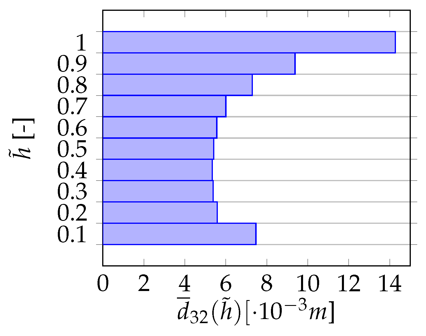
We see that only the smallest bubbles ( mm) escape through the pump outlets, as well as a small amount of the largest bubbles, because of the proximity of the sparger inlet. Immediately after the air enters the absorber sump, a strong reduction in bubble size is observed, which can be attributed to the high shear flow in the area of the agitator and the resulting strong bubble breakup. In the upper part of the absorber sump, the coalescence of the bubbles has a major influence on the bubble size, as a higher proportion of larger bubble size groups can be observed here. The latter is more illustratively shown in Figure 10, where average bubble size (Sauter mean diameter) is plotted against the height of the absorber sump.
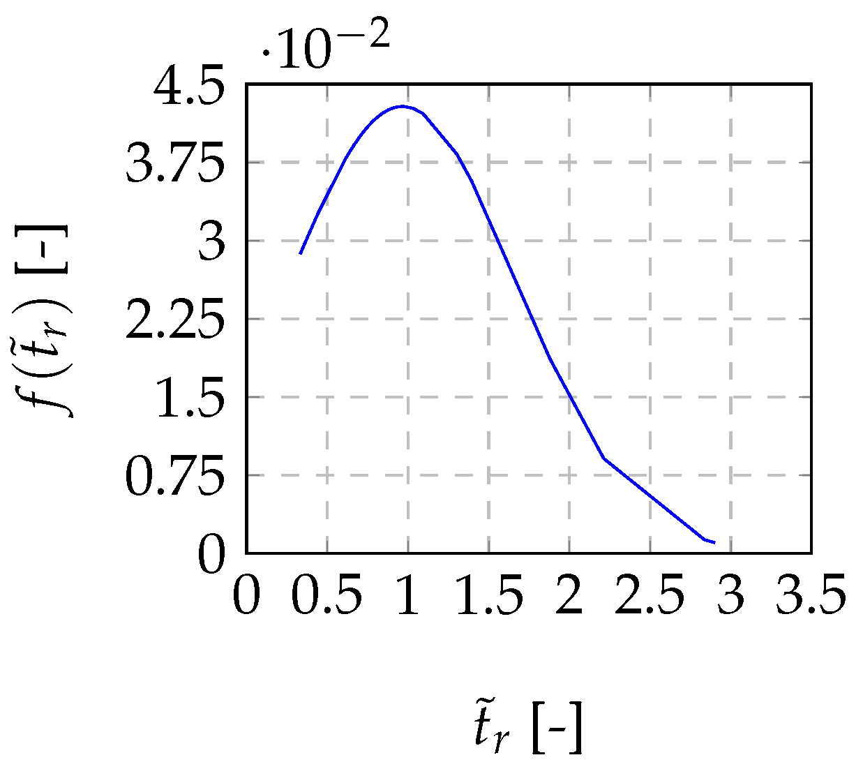
A more detailed analysis of the retention time of the air bubbles was carried out by analyzing the path lines of the air bubbles moving through the absorber sump. The retention time of a single air bubble traveling along the path line () was calculated using a path integral as follows:
By evaluating multiple bubble path lines, a bubble retention time probability function was obtained in non-dimensional form as , as shown in Figure 11. The probability function is expressed by normal distribution as
where is the average non-dimensional bubble retention time, and is its standard deviation.
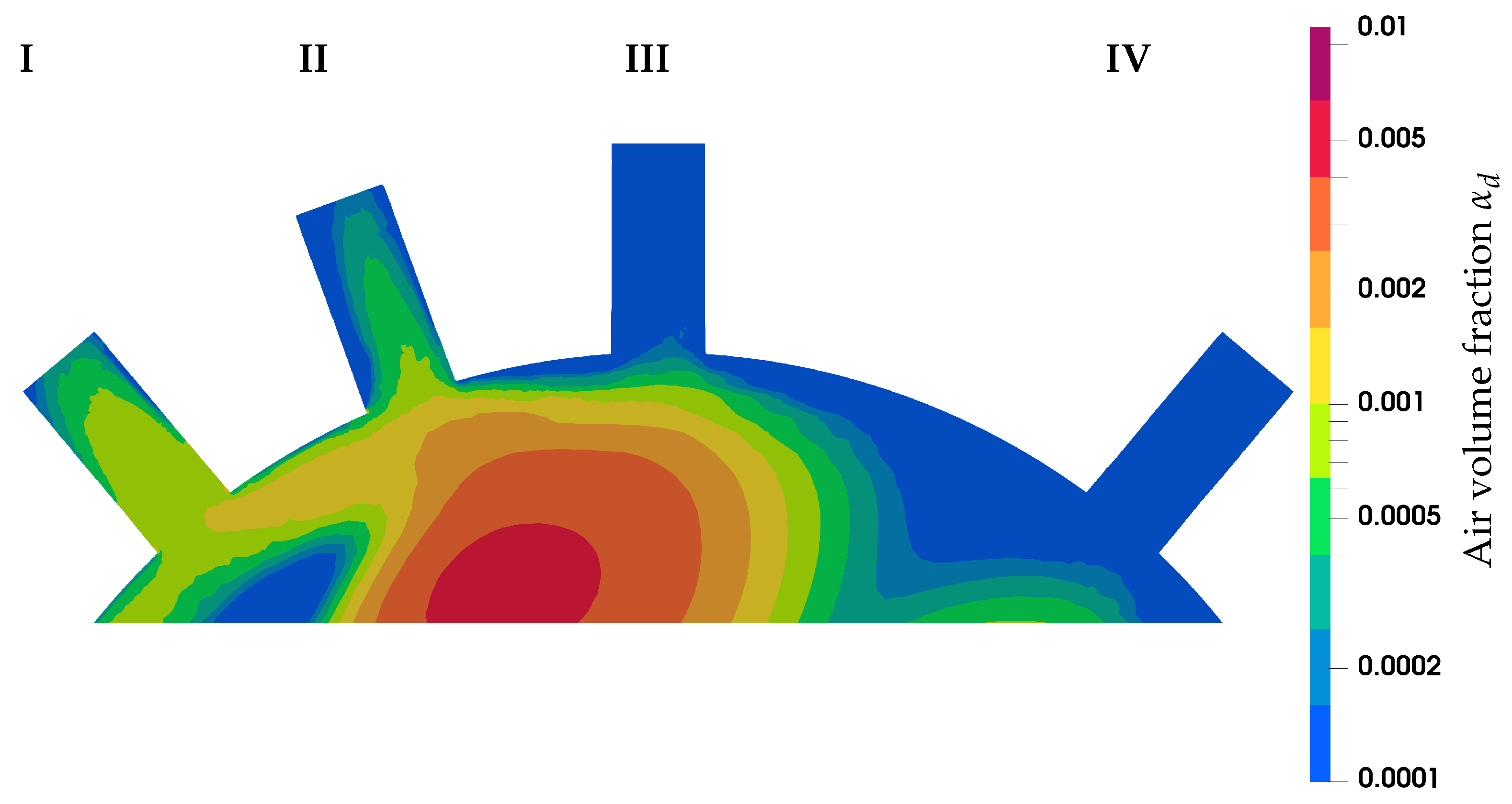
We find that the maximum of the probability function is just below , which implies a good agreement with the calculation of the average retention time based on the bulk volume fraction (). We also observe a relatively large scatter of bubble retention times due to the wide range of bubble diameters, as shown in Figure 11. Figure 12 shows the air volume fraction contours at the pump outlets of the absorber sump as a result of the flow field induced by recirculation pumps.
The total amount of air escaping through the pump outlets accounts for 1.2% of the total air blown into the absorber sump for forced oxidation. Pump outlet no. IV has the least effect on the air distribution in the absorber sump.
4.3. Simulation Results with Lower Linear Momentum Source
An additional operating point was simulated in order to check the FGD absorber sump air dispersion capabilities at lower agitator power. For this simulation, the linear momentum source used to model the influence of the agitators was halved. A comparison of the main process parameters is shown in Table 2.
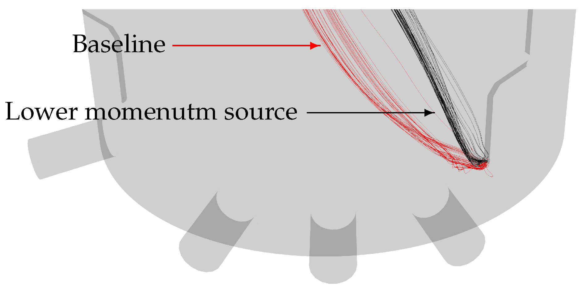
The bulk air volume fraction is lower in the case of a lower momentum source, which is expected. This is due to the air being pushed further towards the center of the absorber sump in the case of the baseline operating point. This phenomenon is better visualized in Figure 13.
The observed phenomenon also affects the escapement of air, as the lower levels of escape are observed in the case of the lowered momentum source.
The remaining process parameters showed no significant change when switching to a lower linear momentum source. The air dispersion is around more homogeneous in the case of the baseline operating point, although it could not entirely be attributed to a lower momentum source. The Sauter mean diameter shows practically no significant difference when comparing the two operating points. However, in real operation, the lower agitator rotor speed would create a lower shear flow and would decrease the rate of bubble breakup in the agitator area. This observation indicates that it would be beneficial to obtain the agitator blade geometry and model the influence of the agitators with the MRF approach.
Table 3 presents a concise overview of the merits and demerits associated with employing numerical modeling in the context of an FGD absorber sump. It highlights the cost-saving aspect of simulations, allowing for efficient exploration of different configurations and providing detailed insights into sump operations. However, it emphasizes the necessity for rigorous model calibration and validation processes to ensure accuracy, especially given the complexity of mathematical modeling involved.
5. Conclusions
Numerical simulation of an FGD absorber sump is able to provide insights into the behavior of the continuous and dispersed phases inside the sump. We have demonstrated that the retention time of the air can be determined in two ways: based on the average volume fraction of the dispersed phase in the sump and by analyzing the path lines of the individual liquid elements (bubbles) leaving the sparger. We found that the retention time deviation of individual bubbles can be large, which is due to a large bubble diameter range. Finally, we analyzed the escape of air through the outlets of the recirculation pumps. We found that the total amount of escaping air is equal to 1.2% of the total air blown into the absorber sump. The escaping air consists mainly of bubbles smaller than 6 mm and is not necessarily lost. On the way through the recirculation pipeline, a transfer of oxygen into the surrounding liquid continues to take place. However this phenomenon should be avoided, since the escaped air has a significantly lower retention time.
A comparison between the two operating points showed that lowering the magnitude of the linear momentum source used for the modeling of agitators results in lower homogeneity and lower air retention time in the absorber sump. However, the Sauter mean diameter of the bubbles changes little between the two operating points. This points to the fact that obtaining the exact geometry of the agitators and modeling their influence with the MRF approach are crucial for the detailed optimization of FGD absorber sumps.
Given the results of the numerical model, optimization of the air spargers can be considered. We observed that the lower part of the absorber sump contains a non-negligible proportion of bubbles larger than 30 mm. Optimization of the air spargers must aim to reduce the bubble diameter at the outlet of the air sparger. Optimization should be carried out in such a way that the pressure drop of the air sparger increases only minimally. The developed numerical model presented in this paper is able to facilitate such optimization and help design the optimal sump.
The technology under consideration requires a flow rate of air blown into the absorber sump with a relative air–CaSO3 ratio of . However, older technology often operates with a relative ratio equal to . In order to fulfill the tender requirements, air turbo-blowers with corresponding motor drives are installed, which enable operation with . By controlling the inlet and diffuser blades of the turbo-blower, the operating point can be lowered to , resulting in a reduction in power consumption of 33%.
The distribution of the dispersed phase and its homogeneity were also determined by numerical calculations. It is important to emphasize that we only modeled the influence of the agitators as a linear momentum source and therefore did not consider the exact geometry of the agitator blades for which the MRF approach would be used. Consequently, the magnitude of the shear stress in the lower part of the absorber sump is lower than it would be if the actual geometry of the agitator blades and the MRF approach were used. In real operation, this increases the proportion of the smallest bubbles and, consequently, the potential escape of air through the outlets of the recirculation pumps. Modeling the agitators as a linear momentum source is a good solution in this case, as obtaining the exact geometry of the agitator blades can be challenging.
The numerical analysis carried out in this study opens up many possibilities for further work. The next stage of numerical modeling of the absorber sump involves the introduction of models for oxygen absorption and the calculation of the mass transfer coefficient. This would allow us to directly determine the amount of oxygen absorbed. By introducing chemical reaction modeling, we could gain insight into the actual amount of oxygen used for forced oxidation. Similar to the absorption process, chemical reactions (oxidation) also take time. Modern and advanced CFD methods already allow for the modeling of chemical reactions, which enables a more precise optimization of the absorber sump and provides more accurate insights into the physical and chemical processes that take place in the absorber sump.
Author Contributions
Conceptualization, J.R.; methodology, N.V.; software, N.V.; validation, N.V.; formal analysis, N.V.; investigation, N.V.; resources, N.V.; data curation, N.V.; writing—original draft preparation, N.V.; writing—review and editing, J.R.; visualization, N.V.; supervision, J.R.; project administration, J.R.; funding acquisition, J.R. All authors have read and agreed to the published version of the manuscript.
Funding
This research was funded by Slovenian research and Innovation Agency (ARIS) grant number P2-0196.
Institutional Review Board Statement
Not applicable.
Data Availability Statement
The data presented in this study are available on request from the corresponding author. The data are not publicly available due to large file size.
Conflicts of Interest
The authors declare no conflict of interest.
Abbreviations
The following abbreviations are used in this manuscript:
| FGD | Flue gas desulfurization |
| CFD | Computational fluid dynamics |
| MRF | Moving reference frame |
| CAD | Computer-aided design |
| URANS | Unsteady Reynolds-averaged Navier–Stokes |
Nomenclature
The following variables and subscripts are used in this manuscript:
| Variable | Meaning | Subscipt | Meaning |
| volume fraction | phase | ||
| density | mass | ||
| t | time | m | momentum |
| velocity vector | j | size group | |
| bubble size deviation | d | dispersed phase | |
| p | pressure | x and y direction | |
| stress tensor | out | outlet | |
| gravitational vector | air | air at the inlet | |
| momentum vector | rel | relative | |
| momentum source vector | i | cell | |
| V | volume | D | drag |
| dynamic viscosity | p | particle | |
| deformation tensor | c | continuous phase | |
| identity matrix | L | lift | |
| N | number concentration | turbulent dispersion | |
| H | source/sink of bubbles | t | turbulent |
| f | proportion of the individual size group of bubbles | virtual mass | |
| n | total number of size groups | wall lubrication | |
| directions | || | tangential | |
| H | height of the absorber sump | without the hydrostatic contribution | |
| flow rate | sim | simulation | |
| F | force magnitude | r | retention |
| force vector | sp | sparger | |
| C | submodel coefficient | q | type of force submodel |
| d | diameter | ||
| Reynolds number | |||
| kinematic viscosity | |||
| Schmidt number | |||
| normal vector | |||
| standard deviation | |||
| non-dimensional height | |||
| A | cross-sectional area | ||
| relative air–CaSO3 ratio | |||
| Weber number | |||
| r | rotation speed | ||
| surface tension | |||
| pathline vector | |||
| Courant number | |||
| D | Diameter |
References
- Mersmann, A.; Kind, M.; Stichlmair, J. Thermal Separation Technology; Springer: Berlin/Heidelberg, Germany, 2011. [Google Scholar] [CrossRef]
- Córdoba, P. Status of Flue Gas Desulphurisation (FGD) Systems from Coal-Fired Power Plants: Overview of the Physic-Chemical Control Processes of Wet Limestone FGDs. Fuel 2015, 144, 274–286. [Google Scholar] [CrossRef]
- de Salazar, R.O.; Ollero, P.; Cabanillas, A.; Otero-Ruiz, J.; Salvador, L. Flue Gas Desulphurization in Circulating Fluidized Beds. Energies 2019, 12, 3908. [Google Scholar] [CrossRef]
- Srivastava, R.K.; Jozewicz, W. Flue Gas Desulfurization: The State of the Art. J. Air Waste Manag. Assoc. 2001, 51, 1676–1688. [Google Scholar] [CrossRef] [PubMed]
- Poullikkas, A. Review of Design, Operating, and Financial Considerations in Flue Gas Desulfurization Systems. Energy Technol. Policy 2015, 2, 92–103. [Google Scholar] [CrossRef]
- Tesárek, P.; Drchalová, J.; Kolísko, J.; Rovnaníková, P.; Černý, R. Flue Gas Desulfurization Gypsum: Study of Basic Mechanical, Hydric and Thermal Properties. Constr. Build. Mater. 2007, 21, 1500–1509. [Google Scholar] [CrossRef]
- Jian, S.; Yang, X.; Gao, W.; Li, B.; Gao, X.; Huang, W.; Tan, H.; Lei, Y. Study on Performance and Function Mechanisms of Whisker Modified Flue Gas Desulfurization (FGD) Gypsum. Constr. Build. Mater. 2021, 301, 124341. [Google Scholar] [CrossRef]
- Navarrete, I.; Vargas, F.; Martinez, P.; Paul, A.; Lopez, M. Flue Gas Desulfurization (FGD) Fly Ash as a Sustainable, Safe Alternative for Cement-Based Materials. J. Clean. Prod. 2021, 283, 124646. [Google Scholar] [CrossRef]
- Arif, A.; Stephen, C.; Branken, D.; Everson, R.; Neomagus, H.; Piketh, S. Modeling Wet Flue Gas Desulfurization. In Proceedings of the Conference of the National Association for Clean Air (NACA 2015), Bloemfontein, South Africa, 1–2 October 2015. [Google Scholar]
- Marocco, L.; Inzoli, F. Multiphase Euler–Lagrange CFD Simulation Applied to Wet Flue Gas Desulphurisation Technology. Int. J. Multiph. Flow 2009, 35, 185–194. [Google Scholar] [CrossRef]
- Qu, J.; Qi, N.; Li, Z.; Zhang, K.; Wang, P.; Li, L. Mass Transfer Process Intensification for SO2 Absorption in a Commercial-Scale Wet Flue Gas Desulfurization Scrubber. Chem. Eng. Process. Process. Intensif. 2021, 166, 108478. [Google Scholar] [CrossRef]
- Qu, J.; Qi, N.; Zhang, K.; Li, L.; Wang, P. Wet Flue Gas Desulfurization Performance of 330 MW Coal-Fired Power Unit Based on Computational Fluid Dynamics Region Identification of Flow Pattern and Transfer Process. Chin. J. Chem. Eng. 2021, 29, 13–26. [Google Scholar] [CrossRef]
- Xiang, L.; Sun, X.; Wei, X.; Wang, G.; Boczkaj, G.; Yoon, J.Y.; Chen, S. Numerical Investigation on Distribution Characteristics of Oxidation Air in a Lime Slurry Desulfurization System with Rotary Jet Agitators. Chem. Eng. Process. Process. Intensif. 2021, 163, 108372. [Google Scholar] [CrossRef]
- Kallinikos, L.; Farsari, E.; Spartinos, D.; Papayannakos, N. Simulation of the Operation of an Industrial Wet Flue Gas Desulfurization System. Fuel Process. Technol. 2010, 91, 1794–1802. [Google Scholar] [CrossRef]
- Gómez, A.; Fueyo, N.; Tomás, A. Detailed Modelling of a Flue-Gas Desulfurisation Plant. Comput. Chem. Eng. 2007, 31, 1419–1431. [Google Scholar] [CrossRef]
- De Blasio, C.; Salierno, G.; Sinatra, D.; Cassanello, M. Modeling of Limestone Dissolution for Flue Gas Desulfurization with Novel Implications. Energies 2020, 13, 6164. [Google Scholar] [CrossRef]
- Höhne, T.; Mamedov, T. CFD Simulation of Aeration and Mixing Processes in a Full-Scale Oxidation Ditch. Energies 2020, 13, 1633. [Google Scholar] [CrossRef]
- Lerotholi, L.; Everson, R.C.; Koech, L.; Neomagus, H.W.J.P.; Rutto, H.L.; Branken, D.; Hattingh, B.B.; Sukdeo, P. Semi-Dry Flue Gas Desulphurization in Spray Towers: A Critical Review of Applicable Models for Computational Fluid Dynamics Analysis. Clean Technol. Environ. Policy 2022, 24, 2011–2060. [Google Scholar] [CrossRef]
- Zhang, G.; Li, Y.; Jin, Z.; Dykas, S.; Cai, X. A Novel Carbon Dioxide Capture Technology (CCT) Based on Non-Equilibrium Condensation Characteristics: Numerical Modelling, Nozzle Design and Structure Optimization. Energy 2024, 286, 129603. [Google Scholar] [CrossRef]
- Zhang, G.; Yang, Y.; Chen, J.; Jin, Z.; Dykas, S. Numerical Study of Heterogeneous Condensation in the de Laval Nozzle to Guide the Compressor Performance Optimization in a Compressed Air Energy Storage System. Appl. Energy 2024, 356, 122361. [Google Scholar] [CrossRef]
- Bricl, M. Cleaning of Flue Gases in Thermal Power Plants. J. Energy Technol. 2016, 9, 45. [Google Scholar]
- Weller, H.G.; Tabor, G.; Jasak, H.; Fureby, C. A Tensorial Approach to Computational Continuum Mechanics Using Object-Oriented Techniques. Comput. Phys. 1998, 12, 620–631. [Google Scholar] [CrossRef]
- Sato, Y.; Sadatomi, M.; Sekoguchi, K. Momentum and Heat Transfer in Two-Phase Bubble Flow—I. Theory. Int. J. Multiph. Flow 1981, 7, 167–177. [Google Scholar] [CrossRef]
- Launder, B.; Spalding, D. The Numerical Computation of Turbulent Flows. Comput. Methods Appl. Mech. Eng. 1974, 3, 269–289. [Google Scholar] [CrossRef]
- Lehnigk, R.; Bainbridge, W.; Liao, Y.; Lucas, D.; Niemi, T.; Peltola, J.; Schlegel, F. An Open-source Population Balance Modeling Framework for the Simulation of Polydisperse Multiphase Flows. Aiche J. 2022, 68, e17539. [Google Scholar] [CrossRef]
- Silva, L.; Lage, P. Development and Implementation of a Polydispersed Multiphase Flow Model in OpenFOAM. Comput. Chem. Eng. 2011, 35, 2653–2666. [Google Scholar] [CrossRef]
- Tomiyama, A.; Tamai, H.; Zun, I.; Hosokawa, S. Transverse Migration of Single Bubbles in Simple Shear Flows. Chem. Eng. Sci. 2002, 57, 1849–1858. [Google Scholar] [CrossRef]
- Burns, A.; Frank, T.; Ian, H.; Shi, J.M. The Favre Averaged Drag Model for Turbulent Dispersion in Eulerian Multi-Phase Flows. In Proceedings of the Conference on Multiphase Flow, ICMF2004, Yokohama, Japan, 30 May–4 June 2004; Volume 392. [Google Scholar]
- Antal, S.; Lahey, R.; Flaherty, J. Analysis of Phase Distribution in Fully Developed Laminar Bubbly Two-Phase Flow. Int. J. Multiph. Flow 1991, 17, 635–652. [Google Scholar] [CrossRef]
Figure 1.
Flow diagram of wet flue gas desulfurization with the main equipment. The flue gas enters the absorber from the side and is diverted upwards. The limestone suspension is sprayed into the counter flow. The gypsum suspension is collected at the bottom of the absorber sump and pumped to a dewatering system.

Figure 2.
Construction of an FGD absorber sump with agitators and spargers. (a) CAD model of the absorber sump with a flue gas inlet duct. In the lower part, the flanges for the installation of the main equipment are also visible. The blue dotted line shows the domain considered in the numerical model. The CAD model was visualized using Solidworks 2023 software. (b) Agitators and spargers inside of the FGD absorber sump in a reference project. In this case, the oxidation air is blown into three points in front of the agitator.

Figure 3.
Boundary conditions of the absorber sump numerical model. Agitators are modeled as a linear momentum source. The free surface enables the outlet of the dispersed phase and the inlet of the continuous phase. The direction of the air inlet is marked with a blue arrow.
Figure 3.
Boundary conditions of the absorber sump numerical model. Agitators are modeled as a linear momentum source. The free surface enables the outlet of the dispersed phase and the inlet of the continuous phase. The direction of the air inlet is marked with a blue arrow.

Figure 4.
Hexagonal mesh of the FGD absorber sump with refinement regions.

Figure 5.
Comparison of bulk air volume fraction for four meshes (, , and cells) with varying element sizes.
Figure 5.
Comparison of bulk air volume fraction for four meshes (, , and cells) with varying element sizes.

Figure 6.
In the lower part of the absorber sump, there is a greater discrepancy in terms of homogeneity between meshes. This can be attributed to a higher gradient of all quantities in this area. (a) Homogeneity of the dispersed air along the height of the absorber sump for different meshes. (b) The gradient magnitude of the dispersed air volume fraction along the height of the absorber sump with the 3 million mesh.

Figure 7.
Contours of the air volume fraction at different heights () of the absorber sump. We can observe the air plume at the inlets of the spargers and the merging of the plumes towards the upper parts of the absorber.
Figure 7.
Contours of the air volume fraction at different heights () of the absorber sump. We can observe the air plume at the inlets of the spargers and the merging of the plumes towards the upper parts of the absorber.

Figure 8.
The 3D contours of the air volume fraction show the movement of air through the absorber sump.
Figure 8.
The 3D contours of the air volume fraction show the movement of air through the absorber sump.

Figure 9.
Contours of the bubble size group fractions on the isosurface of the air volume fraction (). We can see that only the smallest bubbles escape through the pump outlets, as well as a small amount of the largest bubbles, because of the proximity of the sparger inlet. In the upper part, the coalescence of the bubbles has a large influence on the bubble size, as a higher proportion of larger size groups is observed.

Figure 10.
Average bubble Sauter mean diameter along the height of the absorber sump. In the upper part of the absorber sump, the coalescence of the bubbles has a major influence on the bubble size, as a larger average bubble size is observed there.
Figure 10.
Average bubble Sauter mean diameter along the height of the absorber sump. In the upper part of the absorber sump, the coalescence of the bubbles has a major influence on the bubble size, as a larger average bubble size is observed there.

Figure 11.
Bubble retention time probability function. We observe that the maximum of the probability function is around , which implies a good agreement with the average retention time calculated based on the bulk volume fraction (). We also observe relatively scattered bubble retention times, which can be attributed to the wide range of bubble diameters.

Figure 12.
Contours of the air volume fraction at the pump outlets. The largest amount of air escapes through pump outlet no. I. The reason for this lies in the orientation of the agitators, which cause a circular movement of the liquid in the absorber sump, due to which the air plume from the sparger flows directly towards pump outlet no. I.

Figure 13.
The air is being pushed further towards the center of the absorber sump in the case of the baseline operating point. This is due to a higher fluid velocity caused by a higher linear momentum source from the agitator.
Figure 13.
The air is being pushed further towards the center of the absorber sump in the case of the baseline operating point. This is due to a higher fluid velocity caused by a higher linear momentum source from the agitator.


Table 1.
Dispersed-phase size groups.
| Size Group j | Diameter Range (mm) |
|---|---|
| 1 | <3 |
| 2 | |
| 3 | |
| 4 | |
| 5 |
Table 2.
Comparison of the FGD absorber sump air dispersion capabilities at two operating points.
| Baseline | Lower Linear Momentum Source | |
|---|---|---|
| Bulk air vol. frac. ( ) | ||
| Average homogeneity ( ) | ||
| Sauter mean diam. ( [mm]) | ||
| Average escaped air |
Table 3.
Merits and demerits of numerical modeling.
| Merits | Demerits |
|---|---|
| Cost savings | Need for model calibration |
| Quick testing of various configurations | Complex mathematical modeling |
| Detailed insights into sump operation | Extensive data on operating conditions required |
| Enables assessment of failure scenarios | Need for model validation |
Disclaimer/Publisher’s Note: The statements, opinions and data contained in all publications are solely those of the individual author(s) and contributor(s) and not of MDPI and/or the editor(s). MDPI and/or the editor(s) disclaim responsibility for any injury to people or property resulting from any ideas, methods, instructions or products referred to in the content. |
© 2023 by the authors. Licensee MDPI, Basel, Switzerland. This article is an open access article distributed under the terms and conditions of the Creative Commons Attribution (CC BY) license (https://creativecommons.org/licenses/by/4.0/).
Share and Cite
MDPI and ACS Style
Vovk, N.; Ravnik, J. Numerical Modeling of Two-Phase Flow inside a Wet Flue Gas Absorber Sump. Energies 2023, 16, 8123. https://0-doi-org.brum.beds.ac.uk/10.3390/en16248123
AMA Style
Vovk N, Ravnik J. Numerical Modeling of Two-Phase Flow inside a Wet Flue Gas Absorber Sump. Energies. 2023; 16(24):8123. https://0-doi-org.brum.beds.ac.uk/10.3390/en16248123
Chicago/Turabian StyleVovk, Nejc, and Jure Ravnik. 2023. "Numerical Modeling of Two-Phase Flow inside a Wet Flue Gas Absorber Sump" Energies 16, no. 24: 8123. https://0-doi-org.brum.beds.ac.uk/10.3390/en16248123
Note that from the first issue of 2016, this journal uses article numbers instead of page numbers. See further details here.