
Direct Air Cooling of Pipe-Type Transmission Cable for Ampacity Enhancement: Simulations and Experiments


1
Korea Electric Power Corporation (KEPCO) Research Institute, 105 Munjiro, Yuseong, Daejeon 34056, Republic of Korea
2
Department of Mechanical Engineering, Hanbat National University, 125 Dongseodaero, Yuseong, Daejeon 34158, Republic of Korea
*
Author to whom correspondence should be addressed.
Energies 2024, 17(2), 478; https://0-doi-org.brum.beds.ac.uk/10.3390/en17020478
Submission received: 30 November 2023
/
Revised: 26 December 2023
/
Accepted: 16 January 2024
/
Published: 18 January 2024
(This article belongs to the Special Issue Power Transmission and Distribution Equipment and Systems)
Abstract
:Amid the growing demand for energy supply in modern cities, the enhancement of transmission capacity is receiving considerable attention. In this study, we propose a novel method of direct forced cooling in pipe-type transmission lines via an external air supply for reducing the cable temperature and enhancing the ampacity. We conducted numerical simulations using computationally efficient two-dimensional models and a reduced-length three-dimensional model for assessing the cooling efficiency, the distance required for temperature convergence, and the fan/pump capacity required for forced air cooling. We found a 26% increase in ampacity in the case of 5 m/s inlet air velocity into the pipe conduit. We also built and tested the experimental setup equipped with a 300 m length model transmission cable. Results of the forced air cooling experiments show good agreement with numerical simulations. To the best of our knowledge, this study demonstrates the first analysis and validation of direct cooling in pipe-type cables, presenting a promising path for efficient power management in modern metropolitan areas.
1. Introduction
Due to continued urbanization and population growth, energy demand in modern metropolitan areas keeps escalating [1,2,3]. Transmission of electrical energy through the pipe-type power cable [4,5,6] is highly preferred over aerial lines as a means of energy supply to cities, by reasons of its low environmental impact and irrelevance to weather conditions. The current-carrying capacity of a pipe-type transmission cable is affected by various environmental conditions, such as ambient temperature, bonding condition, thermal resistivity, and depth of the pipe burial to the surrounding soil [7]. This is because the heat released from the dielectric loss of the cable, arising from both the conductor and the insulating materials, limits the maximum ampacity of the transmission line. Such Joule heating may result in cable damage and potential thermal runaway upon excessive power transmission. Temperature analysis and control of the pipe-type cable is therefore crucial for safe, efficient, and sustainable transmission of electrical power toward cities [8].
Accordingly, a number of studies have been conducted to analyze the relationship between thermal conditions and the current carrying capacity of the cables. Using the finite element method, Ratchapan et al. [9] analyzed the ampacity of underground low-voltage cables built with various conduit materials. From a similar approach, Al-Dulaimi et al. [10] computed the temperature distribution around the pipe-type underground transmission lines under different thermal conditions. Cable burial depth, thermal resistivity of the soil, the distance between cables, and backfill material types are considered as the varying parameters in their research. Also, Ocłoń et al. [11] proposed and validated a heat transfer model of underground power cables from both finite element simulations and heating experiments. In recent studies, attempts to control the temperature of pipe-type cables to increase the current carrying capacity are being made. For instance, in [12,13], it was shown via numerical simulations that the ampacity of underground power cables can be enhanced by improving the thermal conductivity of the surrounding materials and optimizing the cable-laying method. Furthermore, a numerical study by Kim et al. [14] suggested that the application of thermal interface material within the pipe-type transmission cable can significantly enhance the heat transfer characteristics of the cable and contribute to the ampacity enhancement.
The experimental validation of the cable ampacity enhancement via temperature control, however, is less tackled. In pioneering studies, Kansai Electric Power Company and collaborators [15,16] employed the indirect water cooling system in a 3.4 km long 3-circuit underground transmission line (Nankou-Karyoku line). In that system, water pipes are buried near the cable, and the coolant water is refrigerated in the cooling tower and circled in the closed loop. The performance of the cooling system was measured via an online monitoring system and showed good agreement with mathematical predictions. Subsequently, similar approaches have been made to improve the thermal dissipation characteristics of the transmission cables (e.g., [17]).
Nonetheless, cooling efficiency in existing indirect methods is inherently reduced by thermal resistance between the coolant and the heat source (i.e., conductor). To the best of our knowledge, the method of reducing the temperature of the conductor without heat transfer through such thermal resistance is yet to be developed or tested, either conceptually or experimentally. Focusing on this limitation, we propose in this study a direct air cooling method for reducing the temperature of pipe-type transmission cables and enhancing their ampacity. The proposed method uses air at ambient or refrigerated temperature as the working fluid between the cable and the surrounding pipe. We aim to analyze the cooling effect of the suggested direct forced cooling method via numerical simulations. In addition, we built an on-ground test facility with a 300 m long model cable and a cooling system to validate the proposed method.
The structure of this paper is as follows. We first introduce the proposed cooling method for pipe-type transmission cables in Section 2. We display the details of the numerical simulation and the simulation results in Section 3. Then, we show the experimental setup for validating the present method along with the experiment results in Section 4, before concluding with discussions in Section 5.
2. Forced Air Cooling System
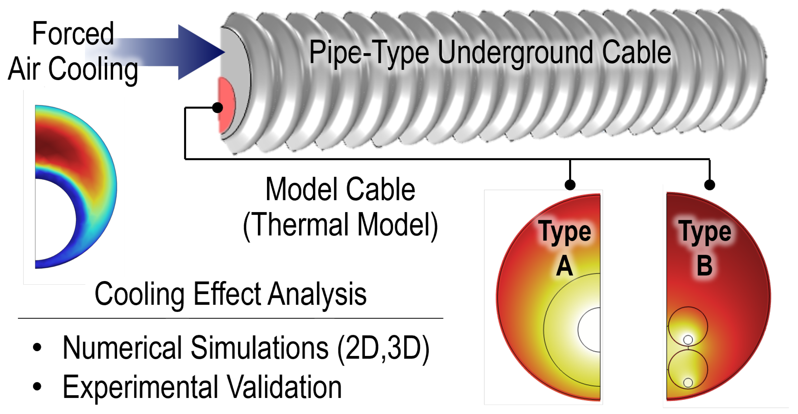
The concept of the proposed forced air cooling method is displayed in Figure 1. In this method, the pipe-type transmission cable is cooled directly via the air, which is in contact with the outer surface of the cable. A space between the cable and the external PVC conduit pipe is used as a cooling channel. Air is supplied by the fan at the pipe inlet, with the optional pump installation at the outlet. The capacity of the fan/pump is deduced from numerical simulations by calculating the pressure drop within the pipe. Two different temperature conditions for inlet air are considered: 20 C (ambient air) and 10 C (refrigerated air). A total cable length of 300 m is used for both the simulation and the experiment.
We consider the 154 kV 2000 mm XLPE cable, which is typical for pipe-type transmission lines, as a target cable to be cooled. We use two different model cables to capture the thermal characteristics of this cable during the power transmission. The first model (type A in Figure 1) is a simplified version of the actual pipe-type transmission cable. The inner part of this model mimics the 154 kV 2000 mm XLPE cable, where thermally negligible cable parts (e.g., metallic sheath and semi-conductive layers) are removed from the model for simplification. This is because, as shown in Table 1, they either have very high thermal conductivity or very small thickness, resulting in negligible thermal resistances. The cooling effect of the actual cable is analyzed with this model. The second model (Type B in Figure 1), on the contrary, is designed for the validation experiment. This model consists of four heat sources enclosed by four inner pipes, whose dimensions and thermal characteristics are shown in Table 1. Four electric heat wires with a maximum temperature of 80 C are used as the heat sources. Despite the discrepancy with the real cable geometry, this type of cable model enables the reproduction of thermal conditions within the pipe conduit without applying electrical power to the actual power cable. The thermal similarity of Type A (actual cable model) and Type B (thermal model) cross-sectional models will be displayed in Section 3.2. Considering the left–right symmetry of the cable models, only half of the cable is modeled and simulated, while the centerline is treated adiabatic.
As mentioned previously in the introduction, the cooling effect of the proposed method is assessed via numerical simulations and the validation experiment. In numerical simulations, we aim to compute the temperature reduction of the model cable and the corresponding increase in ampacity. Because the aspect ratio is very high (the length of the cable is much greater than the diameter), full-scale finite difference analysis is computationally expensive and inefficient. Therefore, we conduct a two-dimensional thermal analysis in the cable cross-section, assuming the thermally fully developed condition. The heat dissipation characteristics of such a model are extracted from reduced-length three-dimensional analysis. As for the validation experiment, we build a test facility with 300 m type B model cable in Korea Electric Power Corporation (KEPCO) Power Testing Center in Gochang, South Korea. An inlet pump connected to the refrigeration system is used to supply the cooling air, and the temperature within the pipe conduit is measured at 30 m intervals. Using this test facility, we compare the temperature before and after the application of the forced air cooling, aiming to evaluate the cooling effect. Further details of the simulation and the experiment will be discussed in Section 3 and Section 4, respectively.
3. Numerical Simulations
3.1. Modeling and Simulation Details
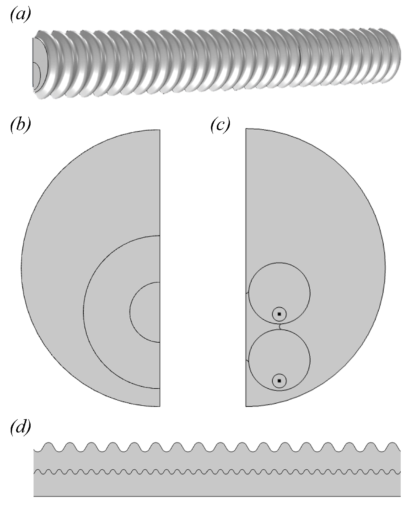
Figure 2 shows the pipe-type transmission cable models used for the present study. First, Figure 2a shows the reduced-length three-dimensional model. Instead of building a full-length (300 m) model, this model has a length of 1.8 m, which is enough for hydrodynamic and thermal development (to be discussed with more details in Section 3.2). The inner part of the pipe conduit consists of the realistic cable model (Type A, Figure 2b) and the experimental model for validation (Type B, Figure 2c), whose geometries were discussed previously in Section 2. The convection heat transfer characteristics of the air between the inner cable and the outer pipe are initially drawn from a three-dimensional model and converted into an equivalent conduction heat transfer coefficient. Finally, Figure 2d shows the axisymmetric pipe-type transmission cable model used for calculating the temperature profile along the cable and the pump capacity required for forced air cooling. The length of the axisymmetric model is set to 300 m. Because of the non-axisymmetricity of the actual transmission line (inner cable located at the pipe bottom due to gravity), we adjust the radius of the pipe conduit, aiming to capture the hydrodynamic and thermal characteristics of the three-dimensional model. The result of such an adjustment will be shown in Section 3.2. The inlet temperatures of the coolant air are set to 10 C and 20 C, and the inlet velocities are set to 0 (natural convection; for reference), 1, 5, and 10 m/s (forced convection). Considering the setup of the validation experiment, the outer boundary of the pipe conduit is considered natural convection with the ambient air.
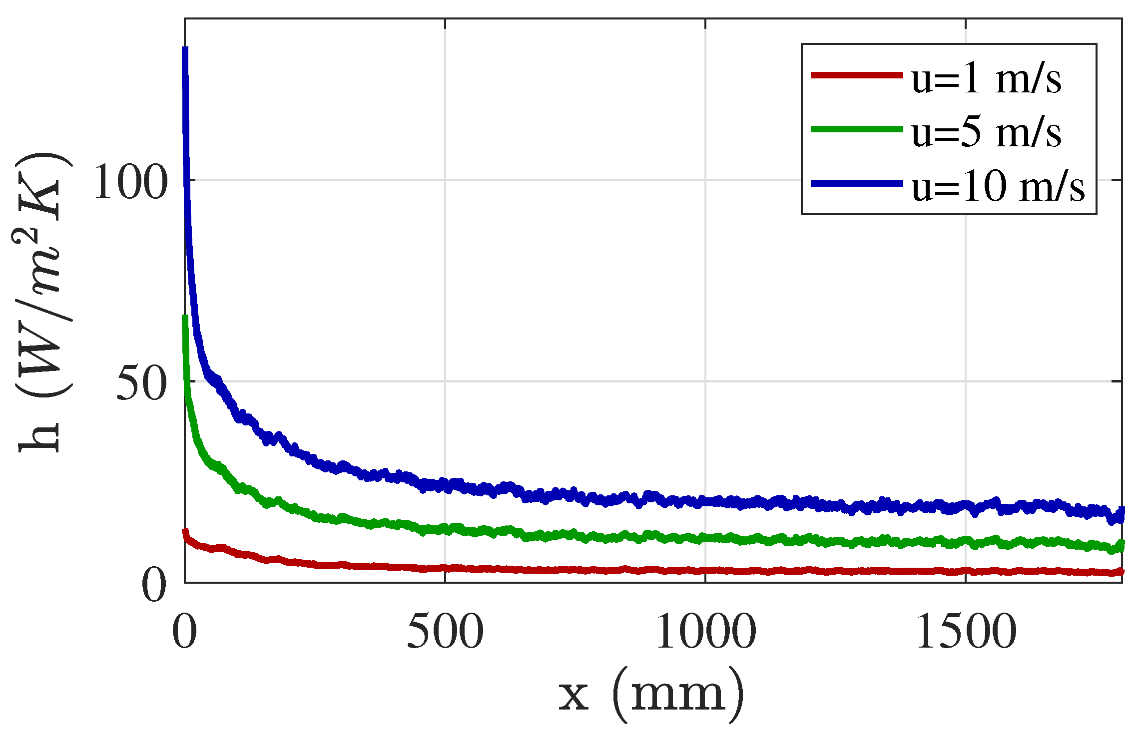
Figure 3 shows the convection heat transfer coefficients at the surface of the inner cable. In all inlet velocities considered, a convergence in the convection heat transfer coefficient is found at around 1 m from the entrance. Therefore, the heat transfer analysis using the two-dimensional cross-sectional model can accurately be conducted by converting the converged convection heat transfer coefficients into the conduction heat transfer coefficient of the air between the inner cable and the outer pipe.
The heat transfer in a three-dimensional model is computed by numerically solving the following governing equations via the finite difference method:
where [J/kg·K] is the specific heat capacity at constant pressure, u [m/s] is the velocity vector, q [W/m] is the heat flux by conduction, k [W/m·K] is thermal conductivity, and T [K] is temperature. [kg/m] is the density computed from the ideal gas assumption (, where [Pa] is the absolute pressure and [J/kg·K] is the specific gas constant). [W/m] is the heating under adiabatic compression, which is equal to , where [1/K] is the thermal expansion coefficient. [W/m] is the viscous dissipation in fluid (). Turbulent fluid flow is modeled using the turbulence model, whose governing equations are left out for brevity. For a two-dimensional model, we alternatively solve the following equations:
where [m] is the thickness of a two-dimensional physical model. Midplanes of the three-dimensional and the cross-sectional model are considered adiabatic (), based on the symmetric geometry. All simulations are conducted in stationary conditions using the COMSOL V6 multiphysics and heat transfer software.
3.2. Simulation Result and Discussion
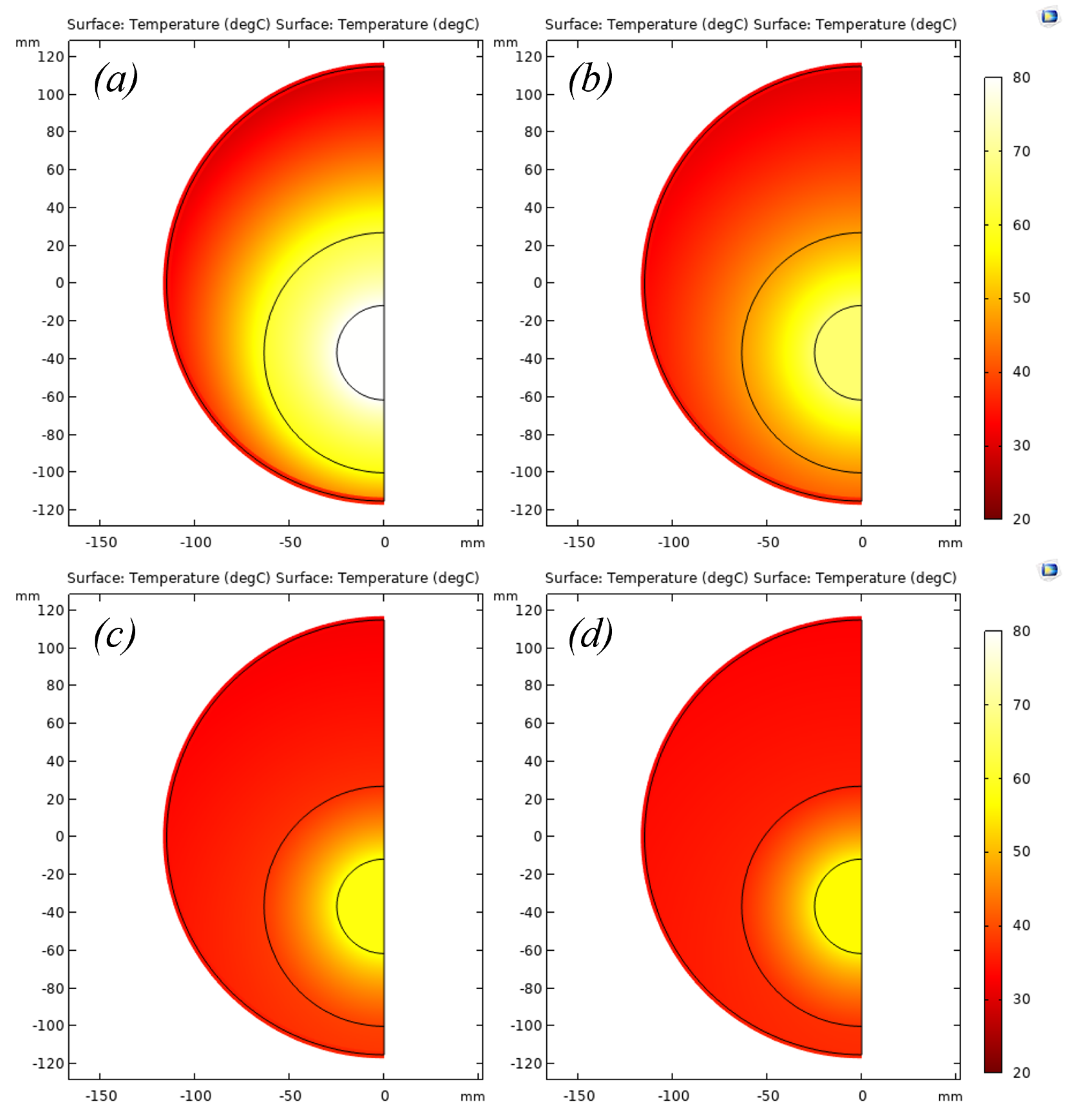
In this section, we describe the results of numerical simulations that used the models that were presented in Section 3.1. The temperature distribution within the pipe-type transmission cable in the realistic model (Type A) with natural and forced air cooling at saturated conditions is shown in Figure 4. In this result, the heat release rate of the conductor is set to a constant, which is equivalent to the temperature of 80 C without forced cooling (Figure 4a). If the temperature of the conductor is fixed, instead of its heat release rate, the maximum heat release rate of the conductor is increased to 128%, 159%, and 165% in case of 1, 5, and 10 m/s inlet air velocities. This is equivalent to the allowance of transmission ampacity of 113%, 126%, and 128%. The result of this fixed-temperature thermal analysis using a cross-sectional model is summarized in Table 2.
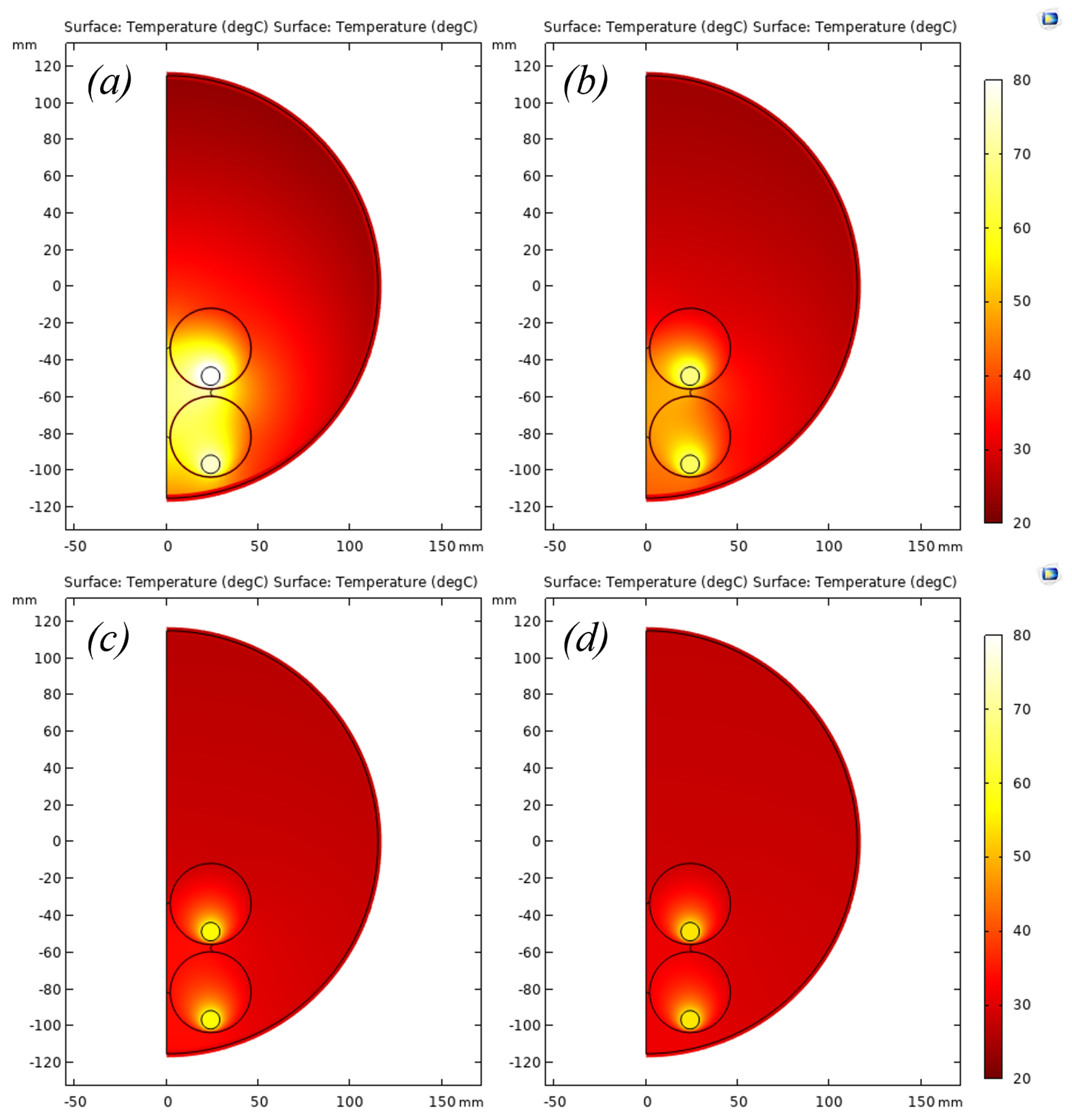
Similar thermal analyses are conducted using the type B cable model, whose results are shown in Figure 5 and Table 3. In the case of fixed conductor temperature at 80 C, the maximum heat release rates of the conductor at the inlet air velocities of 1, 5, and 10 m/s are computed as 129%, 161%, and 163%, which is equivalent to the transmission ampacity of 114%, 127%, and 128%, respectively, compared to the natural convection case. These results are similar to those of the actual cable model (Type A), justifying the efficacy of the validation experiment using the Type B model cable. Specifically, conductor heat loss (q) and the maximum current allowance (I) of two models (Type A, Type B) differed no more than two and one percentage points, respectively, as can be found from Table 2 and Table 3. In both types of the cable model, we found that a significant increase of the maximum heat release rate and the transmission ampacity is achieved until the inlet air velocity of 5 m/s, while just a little enhancement in cooling effect was achieved upon a further increase of air velocity to 10 m/s. Therefore, we concluded that the forced air cooling with the inlet air velocity no greater than 5 m/s should be adopted for efficient cooling. It is worth mentioning that the results of the simulations are obtained under the standard ambient air condition (20 C), and the efficiency of the cable cooling may vary upon different environmental conditions.
The next question that can be naturally asked would be, at which point are the cross-sectional temperature profiles shown in Figure 4 and Figure 5 found? Although the convective heat transfer characteristics at the outer boundary of the inner cable converge at around 1 m from the inlet (see Figure 3), the convergence in temperature profile is achieved at much downstream. We use the 300 m length axisymmetric cable model (Figure 2d) to find the convergence in temperature. Specifically, we find the position where the first decimal of the average coolant air temperature (T, in C) does not change for at least one meter in the flow direction, and define that position as the temperature converging point. Considering the simulation results in the previous paragraph, we exclude the inlet air velocity of the 10 m/s case and analyze 0 (natural convection), 1, and 5 m/s (forced convection) cases only. The result of the convergence analysis using the axisymmetric cable model is shown in Table 4. In the forced cooling case using the ambient air (20 C), the temperature convergence was made close to the pipe entrance (11.8 m and 10.3 m for 1 m/s and 5 m/s inlet air velocities, respectively), and the distance required for the convergence was similar to the natural convection case (11.1 m). On the contrary, refrigerated air cooling (10 C) cases showed longer distance for the temperature convergence, requiring 40.2 m and 75.0 m in 1 m/s and 5 m/s inlet air velocities, respectively.
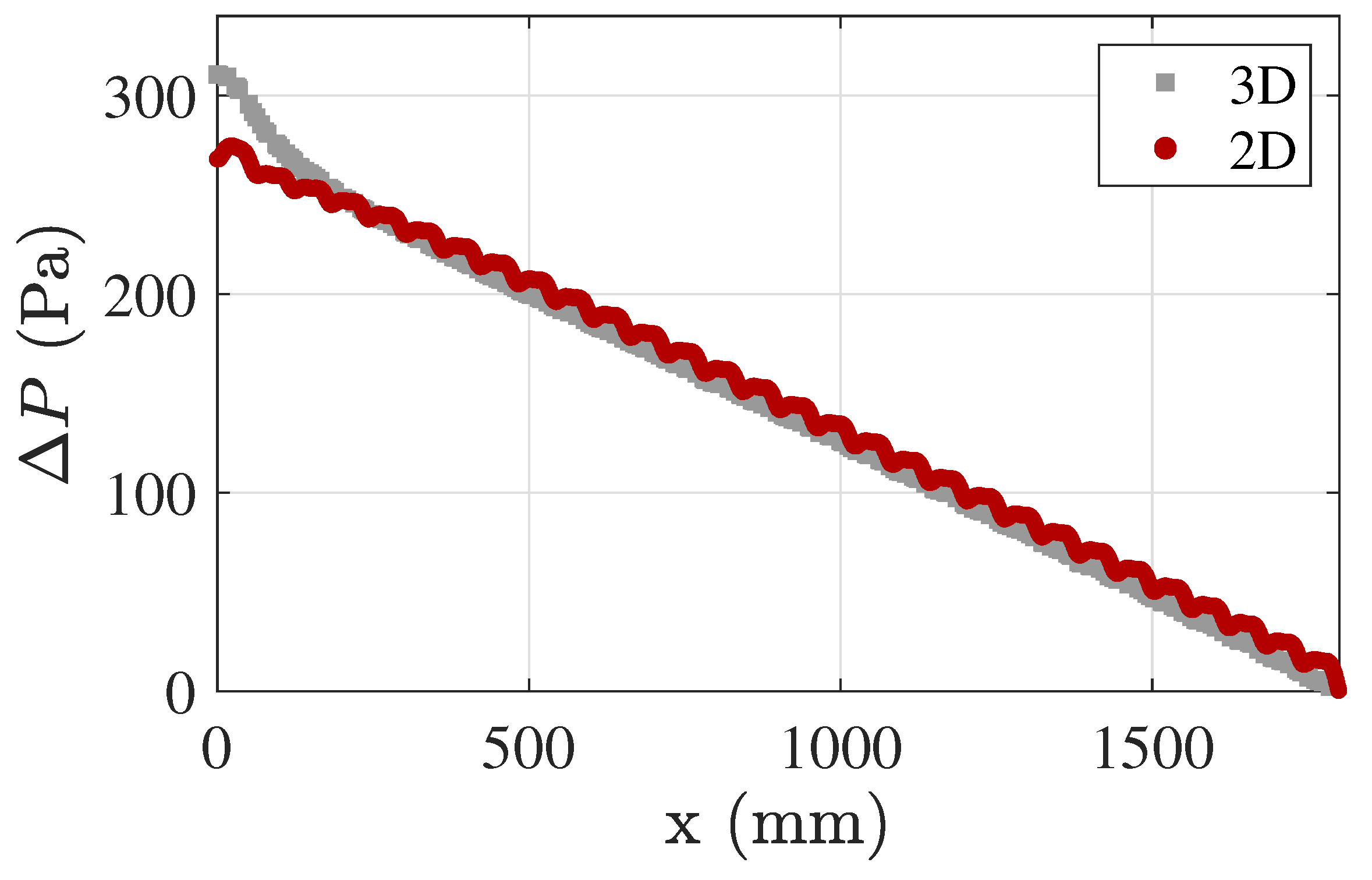
Finally, we determine the fan/pump capacity required for the air supply by computing the pressure drop within the pipe conduit. We first compute the pressure drop using the reduced-length three-dimensional model (Figure 2a) and the axisymmetric model (Figure 2d). Then, we adjust the diameter of the axisymmetric model to match the pressure gradient () of the three-dimensional model (see Figure 6). The Type A cable model is used in the three-dimensional model for this analysis because it requires higher fan/pump power compared to the Type B model. Finally, using the diameter-adjusted axisymmetric model, we conduct the pressure drop analysis of the full-length pipe model. From the pressure difference between the pipe inlet and outlet ( [Pa]), we compute the fan/pump capacity (Q [W]) using the following relationship:
where is the non-dimensional fan efficiency and [m/s] is the volume flow rate of the air. Among the general fan efficiency 0.4–0.6, we select the harsh condition 0.4 for the analysis. Also, we give the safety factor of 2 to compensate for the simplified geometry of the pipe conduit (e.g., pipe curvature [19], surface roughness [20], compressibility of the air [21], hydrodynamic instability and turbulence [22,23], etc.). As a result, in the 1 m/s inlet air velocity case, a pressure drop of 2.74 Pa/m is deduced from the simulation, which can be converted into 0.128 kW fan/pump power for 300 m pipe conduit. Similarly, in the 5 m/s inlet air velocity case, pressure drop and fan/pump power are computed as 41.81 Pa/m and 9.78 kW, respectively. Despite the minor increase in cooling effect, a much higher fan/pump power of 69.93 kW was required in the 10 m/s inlet air velocity case, reassuring our previous conclusion that an inlet air velocity greater than 5 m/s is inefficient. The fan/pump capacity calculated here can be carried solely by a fan at the pipe inlet or a pump at the pipe outlet. Also, both fan and pump can be installed at the pipe inlet and outlet, carrying half the required capacity each.
4. Experimental Validation
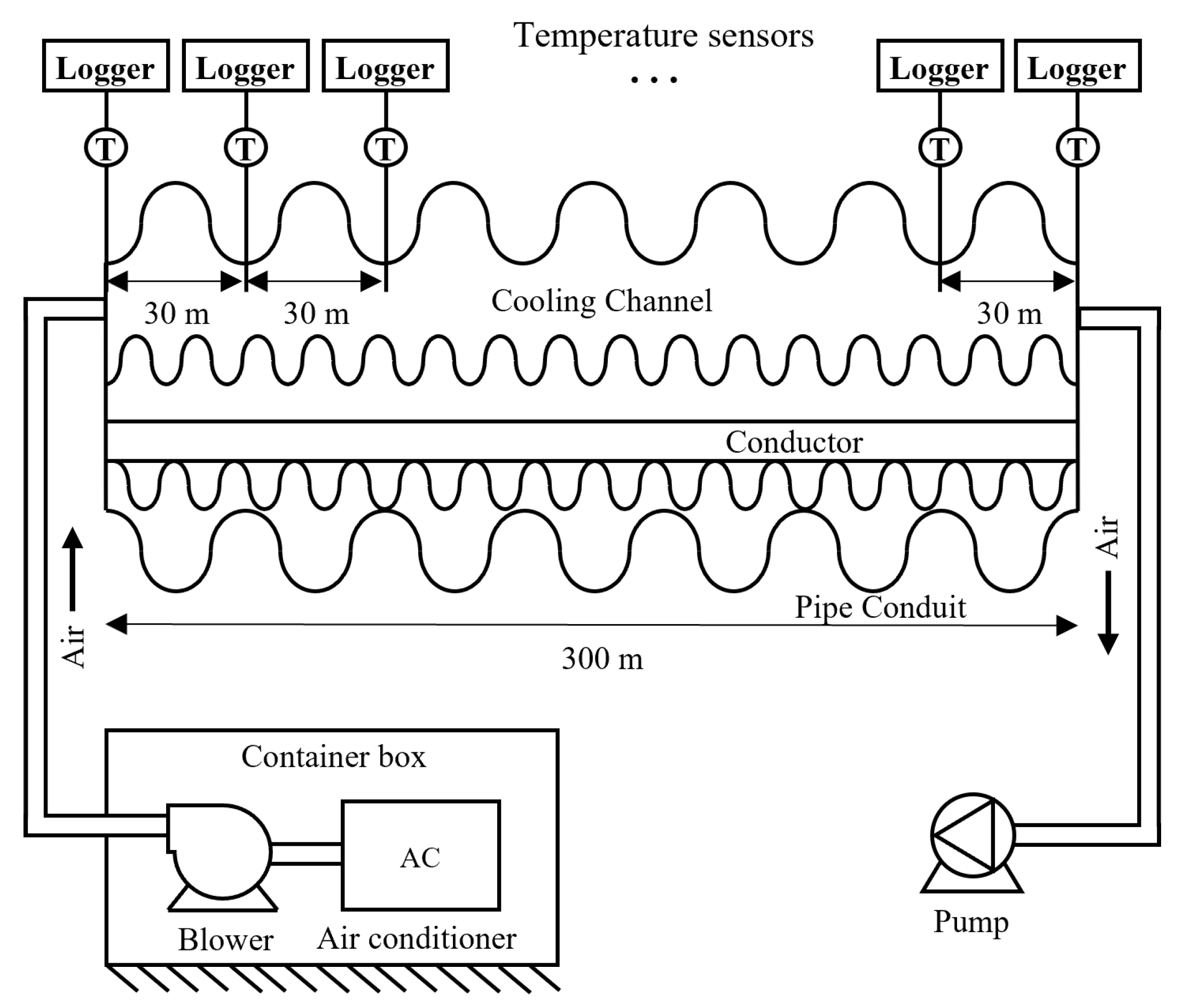
We now present the experimental setup and results for validating the thermal models and the analysis results displayed in Section 3. Figure 7 shows the schematic of the test facility installed in KEPCO Power Testing Center in Gochang, Republic of Korea, for the validation of the proposed cable cooling method. The coolant air is supplied into the cooling channel between the inner pipe and the outer pipe conduit. The temperature of the coolant air is controlled by the air conditioner (Carrier CP-2005AXA). The blower at the air inlet and pump at the outlet (Hwanghae HRB-700 three-phase ring blower motor) are designed to circulate the air at a constant rate. In every test condition, we operate the cooling system for over 300 consecutive minutes before measuring the temperature of the pipe conduit for sufficient thermal convergence.
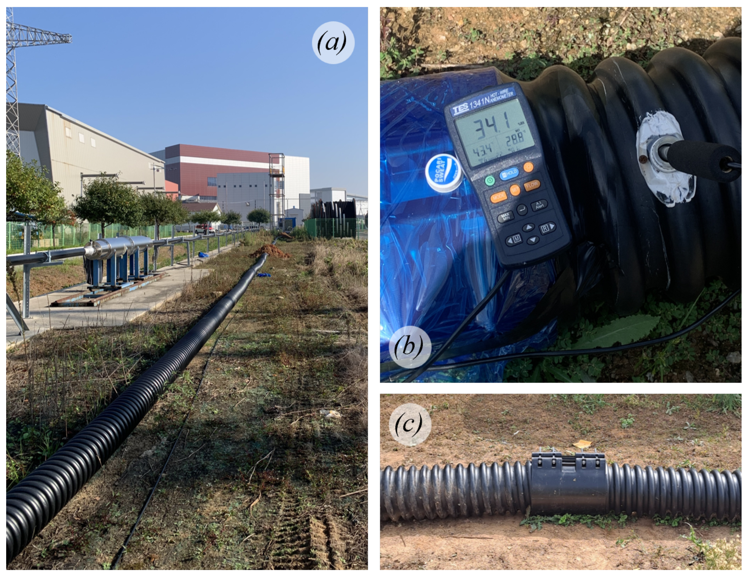
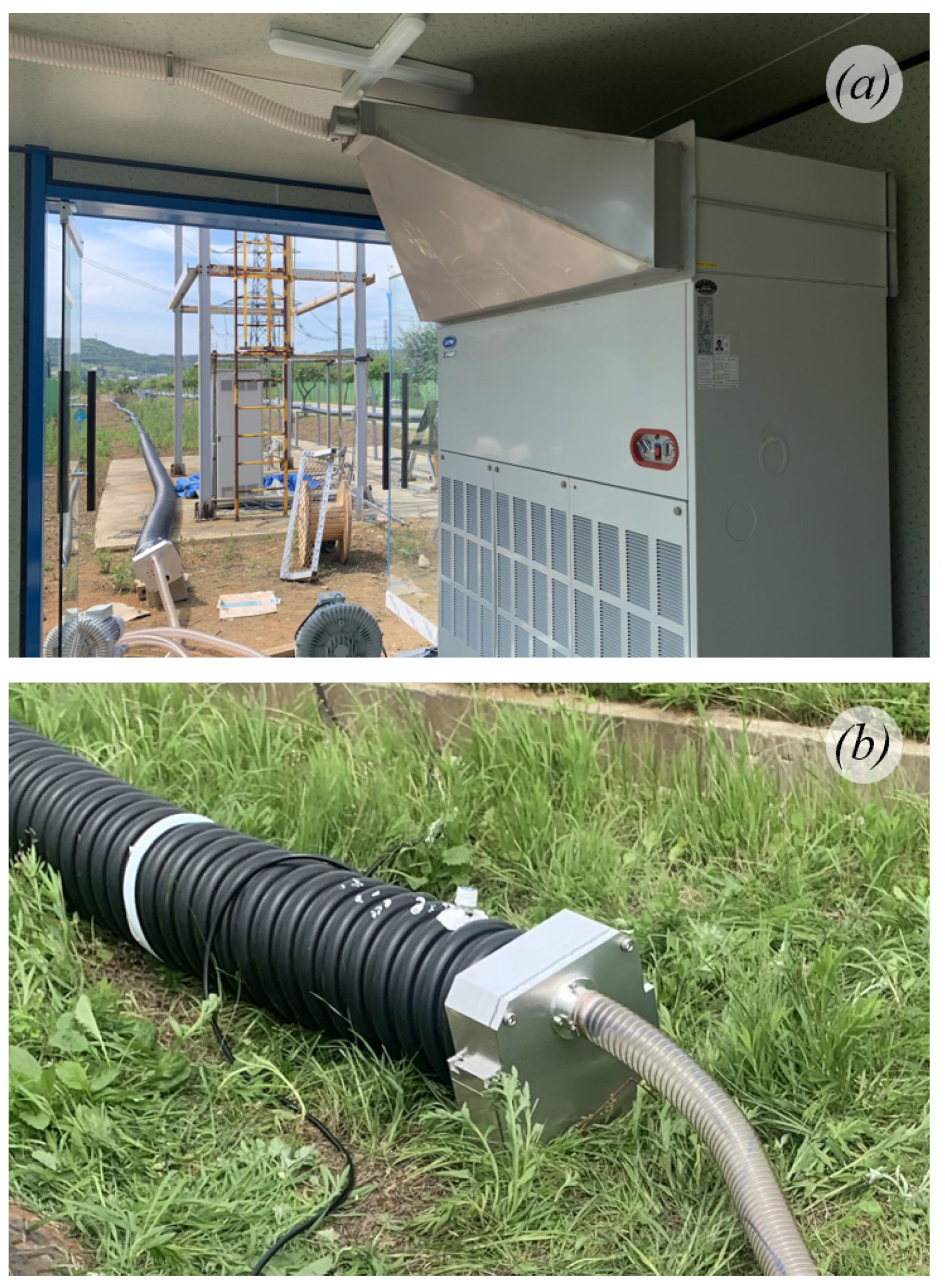
The sub-figures of Figure 8 show the pictures of the validation test facility. By connecting ten 30 m pipe conduits (Figure 8c), a full-length model transmission cable with a total length of 300 m is built (Figure 8a). Type B model cable is installed within the pipe conduit, and the air temperature at the middle of the inner and outer pipe is recorded every 30 m (Figure 8b). Air velocity and temperature are measured using hot-wire anemometer (TES-1341N with flexible probe, precision m/s and ).
In order to perfectly reproduce the environmental condition of the test site via the numerical simulation framework introduced in Section 3, we adjust the ambient temperature condition of the numerical model. Specifically, we recognize that the atmospheric temperature measured at the test site (33 C) is much higher than the standard air condition assumed in Section 3 (20 C), and use the former temperature for the additional analysis. As a result, we were able to capture the thermal characteristics of the validation experiment with the updated numerical model, where the air temperature within the pipe conduit was 47 C without air cooling. All other conditions and simulation details, such as dimensions, thermal properties, and boundary conditions, are kept identical to the framework described in Section 3.
As mentioned above, we reduced the temperature of the coolant air using the refrigerator (Figure 9a). The cooled air is then supplied into the pipe conduit via the interface device (Figure 9b). The temperature and velocity of the coolant air measured at the pipe inlet were 18 C and 4 m/s, respectively. The cooling effect of the direct air cooling with ambient (33 C) air at the same environmental condition is assessed by numerical simulation only.
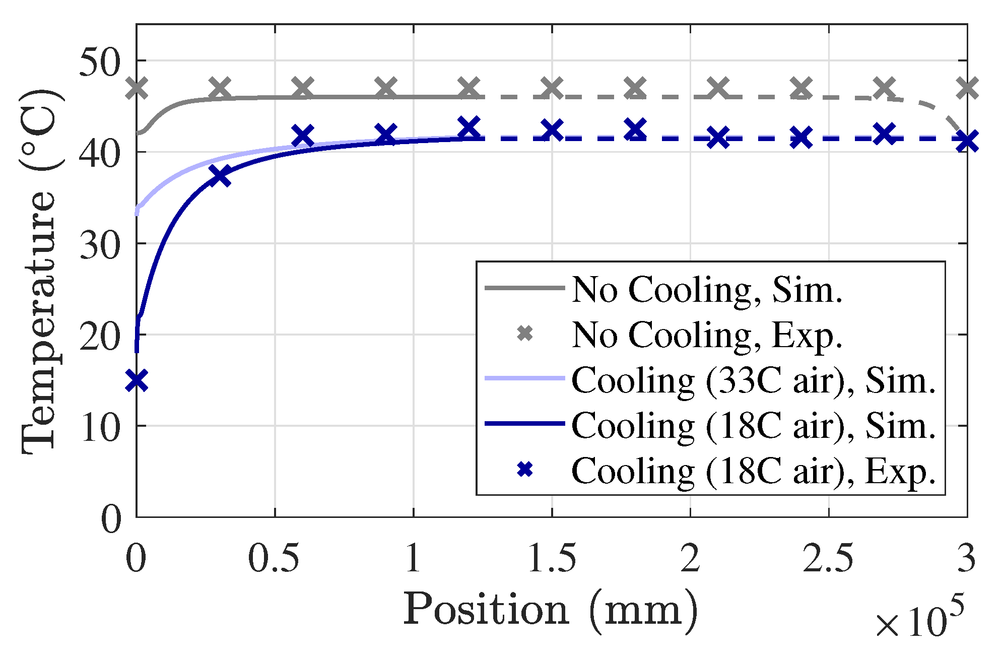
Figure 10 shows the results of the validation experiment and its comparison to the simulation results. Because the increment in heat release rate and current-carrying capacity shown in Table 2 and Table 3 are difficult to be experimentally measured, we alternatively validate the numerical model by measuring the decrease in air temperature within the pipe conduit. In the experiment, the air temperature dropped from 47 C to 41.6–42.7 C after applying the forced air cooling in the converged situation, marking the saturated average temperature of 42.0 C. The convergence in temperature was reached between 60 m and 90 m from the pipe inlet. The results of the validation experiment well match the numerical simulation results, in terms of temperature and convergence characteristics, confirming the reliability of the numerical simulations conducted in the present study. Specifically, the simulation results show that the air temperature within the pipe converges to 46.0 C and 41.4 C before and after the air cooling with 18 C air, respectively. These simulation results, in absolute temperature, indicate the deviation of 0.4% and 0.2% from the experimental observation. Thus, we could conclude that the cable temperature reduction and the ampacity enhancement from the direct pipe air cooling computed in Section 3 are sufficiently reliable.
5. Conclusions
In this study, we proposed a novel direct cooling method for the pipe-type transmission cable to improve the cable’s heat transfer characteristics, leading to ampacity enhancement. We conducted numerical simulations using a realistic cable model and a validating experimental model. From the two-dimensional cross-sectional analysis in the fully developed condition, we found an ampacity increase of 13–28% in both models, depending on the inlet air velocity. We also computed the distance for temperature convergence and fan/pump capacity using an axisymmetric cable model. We verified the reliability of the numerical simulations via the full-scale (300 m) experiment, whose results showed a good match with the simulation results. This study constitutes the first attempt in direct air cooling of pipe-type transmission cables, to the best of our knowledge.
There are several important implications of the present study. First, we have proposed a novel method for analyzing the cooling effect of the transmission cable. This method consists of (1) reduced-length three-dimensional analysis for extracting the heat transfer characteristics of the cable, (2) cross-sectional analysis in thermally converged conditions, and (3) axisymmetric analysis for computing the distance until convergence. Such a series of analyses enables the accurate estimation of the cooling effect without requiring computationally expensive full-scale three-dimensional simulations. Second, we have conducted a full-scale experiment to validate the direct cooling method. In line with the analysis method described above, the validation experiment can ensure the reliability of the numerical simulations on cable cooling. Finally, unlike the existing cable-cooling methods (e.g., water cooling via pipe burial), the proposed direct cooling system does not require additional installation of the cooling line alongside the pipe conduit. Instead, only the air blowers with optional air conditioners at every 300 m of the transmission line are required. This allows for the efficient installation and operation of the cable cooling system, from both engineering and economic points of view.
Several improvements in the simulation and experiment of the present method can be made through future studies. First, every simulation in this study is performed in the stationary condition. Therefore, the temperature measurements in the validation experiment were conducted after sufficient time since the heat application. This is because the present study focuses on the assessment of the maximum ampacity increment, rather than time-varying cooling performance. In the actual transmission cables, however, it might also be important to assess how fast the cooling system can reduce the temperature of the transmission cables. Furthermore, in practical transmission occasions, the heat release rate of the cable can vary over time. Thus, one can conduct the transient heat transfer analysis in future studies. Second, in both the numerical and experimental analysis of this study, we used cable models that are thermally equivalent to the actual transmission cable. Further experimental validation of the present cooling method can be conducted using an actual power transmission cable, e.g., the 154 kV XLPE cable simulated in this study. Finally, pipe-type transmission cables are majorly used for underground applications. Although not shown in this study because of experimental limitations, future research can be conducted in an underground environment [24,25].
Author Contributions
Conceptualization, D.-K.K. and Y.-W.K.; methodology, D.-K.K. and Y.-W.K.; software, J.G.K. and M.L.; validation, D.-K.K. and H.-R.J.; formal analysis, J.G.K. and M.L.; investigation, all Authors; resources, Y.-W.K. and M.L.; data curation, D.-K.K. and M.L.; writing, M.L.; funding acquisition, D.-K.K. and Y.-W.K. All authors have read and agreed to the published version of the manuscript.
Funding
This study was supported by the Korea Electric Power Corporation (development of cooling technology to increase the power transmission capacity of underground cables in ducts, project No. R21TA22).
Institutional Review Board Statement
Not applicable.
Informed Consent Statement
Not applicable.
Data Availability Statement
Data availability will be reviewed by the KEPCO research institute upon request.
Conflicts of Interest
The authors declare no conflicts of interest.
References
- Kwasiborska, A.; Stelmach, A.; Jabłońska, I. Quantitative and Comparative Analysis of Energy Consumption in Urban Logistics Using Unmanned Aerial Vehicles and Selected Means of Transport. Energies 2023, 16, 6467. [Google Scholar] [CrossRef]
- Lai, C.M.; Teh, J. Comprehensive review of the dynamic thermal rating system for sustainable electrical power systems. Energy Rep. 2022, 8, 3263–3288. [Google Scholar]
- Juan, A.A.; Ammouriova, M.; Tsertsvadze, V.; Osorio, C.; Fuster, N.; Ahsini, Y. Promoting Energy Efficiency and Emissions Reduction in Urban Areas with Key Performance Indicators and Data Analytics. Energies 2023, 16, 7195. [Google Scholar]
- Xu, X.B.; Liu, G. Investigation of the magnetic field produced by unbalanced phase current in an underground three-phase pipe-type cable. Electr. Power Syst. Res. 2002, 62, 153–160. [Google Scholar] [CrossRef]
- Li, B.; Ding, Y.; Du, Y.; Chen, M. Stable thin-wire model of buried pipe-type power distribution cables for 3D FDTD transient simulation. IET Gener. Transm. Distrib. 2020, 14, 6168–6178. [Google Scholar] [CrossRef]
- Brignone, M.; Mestriner, D.; Molfino, P.; Nervi, M.; Marzinotto, M.; Patti, S. The Mitigation of Interference on Underground Power Lines Caused by the HVDC Electrode. Energies 2023, 16, 7769. [Google Scholar] [CrossRef]
- De León, F. Major factors affecting cable ampacity. In Proceedings of the 2006 IEEE Power Engineering Society General Meeting, Montreal, QC, Canada, 18–22 June 2006; pp. 1–6. [Google Scholar]
- Xiao, R.; Liang, Y.; Fu, C.; Cheng, Y. Rapid calculation model for transient temperature rise of complex direct buried cable cores. Energy Rep. 2023, 9, 306–313. [Google Scholar] [CrossRef]
- Ratchapan, R.; Kongjeen, Y.; Plangklang, B. Ampacity Analysis of Low Voltage Underground Cables in Different Conduits. In Proceedings of the 2021 9th International Electrical Engineering Congress (iEECON), Pattaya, Thailand, 10–12 March 2021; pp. 25–28. [Google Scholar]
- Al-Dulaimi, A.A.; Güneşer, M.T.; Hameed, A.A. Investigation of thermal modeling for underground cable ampacity under different conditions of distances and depths. In Proceedings of the 2021 5th International Symposium on Multidisciplinary Studies and Innovative Technologies (ISMSIT), Ankara, Turkey, 21–23 October 2021; pp. 654–659. [Google Scholar]
- Ocłoń, P.; Pobędza, J.; Walczak, P.; Cisek, P.; Vallati, A. Experimental validation of a heat transfer model in underground power cable systems. Energies 2020, 13, 1747. [Google Scholar] [CrossRef]
- Xu, X.; Yuan, Q.; Sun, X.; Hu, D.; Wang, J. Simulation analysis of carrying capacity of tunnel cable in different laying ways. Int. J. Heat Mass Transf. 2019, 130, 455–459. [Google Scholar]
- Che, C.; Yan, B.; Fu, C.; Li, G.; Qin, C.; Liu, L. Improvement of cable current carrying capacity using COMSOL software. Energy Rep. 2022, 8, 931–942. [Google Scholar]
- Kim, J.G.; Sohn, S.H.; Lim, J.H.; Shim, M.J.; Lee, M. Numerical study on the ampacity enhancement of pipe-type underground transmission cable through the thermal interface material. Trans. Korean Soc. Mech. Eng. 2024, 48. [Google Scholar]
- Hayashi, M.; Uchida, K.; Kumai, W.; Sanjo, K.; Mitani, M.; Ichiyanagi, N.; Goto, T. Development of water pipe cooling system for power cables in tunnels. IEEE Trans. Power Deliv. 1989, 4, 863–872. [Google Scholar] [CrossRef]
- Kumai, W.; Hashimoto, I.; Ohsawa, S.; Mitani, M.; Matsuda, Y. Completion of high-efficiency water pipe cooling system for underground transmission line. IEEE Trans. Power Deliv. 1994, 9, 585–590. [Google Scholar]
- Joyce, R.; Lloyd, S. Indirect pipe water cooling study for a 220 kV underground XLPE cable system in New Zealand. In Proceedings of the International Conference on Insulated Power Cables, Paris, France, 21–25 June 2015; pp. 1–6. [Google Scholar]
- Wei, Y.; Liu, M.; Li, X.; Li, G.; Li, N.; Hao, C.; Lei, Q. Effect of temperature on electric-thermal properties of semi-conductive shielding layer and insulation layer for high-voltage cable. High Volt. 2021, 6, 805–812. [Google Scholar]
- Berger, S.A.; Talbot, L.; Yao, L.S. Flow in curved pipes. Annu. Rev. Fluid Mech. 1983, 15, 461–512. [Google Scholar]
- Farshad, F.F.; Rieke, H.H. Surface-roughness design values for modern pipes. SPE Drill. Complet. 2006, 21, 212–215. [Google Scholar] [CrossRef]
- Konrad, K. Dense-phase pneumatic conveying through long pipelines: Effect of significantly compressible air flow on pressure drop. Powder Technol. 1986, 48, 193–203. [Google Scholar] [CrossRef]
- Lee, M.; Zhu, Y.; Li, L.K.B.; Gupta, V. System identification of a low-density jet via its noise-induced dynamics. J. Fluid Mech. 2019, 862, 200–215. [Google Scholar]
- Park, S.; Lee, M. A semi-supervised framework for analyzing the potential core of a low-density jet. Flow Meas. Instrum. 2024, 95, 102516. [Google Scholar] [CrossRef]
- Olsen, R.; Anders, G.J.; Holboell, J.; Gudmundsdóttir, U.S. Modelling of dynamic transmission cable temperature considering soil-specific heat, thermal resistivity, and precipitation. IEEE Trans. Power Deliv. 2013, 28, 1909–1917. [Google Scholar] [CrossRef]
- Ocłoń, P.; Cisek, P.; Pilarczyk, M.; Taler, D. Numerical simulation of heat dissipation processes in underground power cable system situated in thermal backfill and buried in a multilayered soil. Energy Convers. Manag. 2015, 95, 352–370. [Google Scholar] [CrossRef]
Figure 1.
Schematic of the forced air cooling method applied on the model transmission cable. For dimensions of the cross sections, see Table 1.
Figure 1.
Schematic of the forced air cooling method applied on the model transmission cable. For dimensions of the cross sections, see Table 1.

Figure 2.
(a) Reduced-length (1.8 m) three-dimensional cable model. (b) Type A and (c) Type B two-dimensional cross-sectional cable model. (d) Axisymmetric cable model (partially displayed). See Table 1 for the dimensions of cross-sectional cable models.
Figure 2.
(a) Reduced-length (1.8 m) three-dimensional cable model. (b) Type A and (c) Type B two-dimensional cross-sectional cable model. (d) Axisymmetric cable model (partially displayed). See Table 1 for the dimensions of cross-sectional cable models.

Figure 3.
Convective heat transfer coefficient (h) at the cable surface obtained at various inlet air velocities (u) via numerical simulations in 3D cable model (Figure 2d). The dependence on inlet temperature is found to be negligible.
Figure 3.
Convective heat transfer coefficient (h) at the cable surface obtained at various inlet air velocities (u) via numerical simulations in 3D cable model (Figure 2d). The dependence on inlet temperature is found to be negligible.

Figure 4.
Temperature distribution within Type A model cable (a) before and (b–d) after the application of direct forced air cooling. The heat release rate from the conductor is kept constant, which is equivalent to the temperature of 80 C in subfigure (a). Inlet air velocity (u) is set to (b) 1 m/s, (c) 5 m/s, and (d) 10 m/s. Hydrodynamically and thermally fully-developed condition is assumed.

Figure 5.
Temperature distribution within Type B model cable (a) before and (b–d) after the application of direct forced air cooling. The heat release rate from the conductor is kept constant, which is equivalent to the temperature of 80 C in subfigure (a). Inlet air velocity (u) is set to (b) 1 m/s, (c) 5 m/s, and (d) 10 m/s. Hydrodynamically and thermally fully-developed condition is assumed.

Figure 6.
Comparison of the pressure drop characteristics () within the reduced-length three-dimensional cable model (Figure 2a, grey squares) and the two-dimensional axisymmetric cable model (Figure 2d, red circles).

Figure 7.
Schematic diagram (not to scale) of the direct air cooling test facility installed in KEPCO Power Testing Center.
Figure 7.
Schematic diagram (not to scale) of the direct air cooling test facility installed in KEPCO Power Testing Center.

Figure 8.
Pictures showing (a) the model cable installed in the test site, (b) the air temperature measurement within the model cable, and (c) the connection between pipe conduit segments.
Figure 8.
Pictures showing (a) the model cable installed in the test site, (b) the air temperature measurement within the model cable, and (c) the connection between pipe conduit segments.

Figure 9.
Pictures showing (a) air supply at the entrance of the pipe conduit and (b) refrigeration of the supplied air.
Figure 9.
Pictures showing (a) air supply at the entrance of the pipe conduit and (b) refrigeration of the supplied air.

Figure 10.
Air temperature within the pipe conduit before (grey) and after (blue) the application of direct forced cooling. Cross markers show experimental measurements and solid lines show numerical simulation results. Dashed lines are assumptions derived from the symmetry of the cable (no cooling case) and saturation of the temperature profile (cooling cases).


Table 1.
Material, inner diameter, thickness, and thermal conductivity of the materials used for simulation and experiment. SC Layer denotes the semi-conductive layer, whose thermal conductivity is shown in [18]. * Metallic sheath and SC layers are neglected in the numerical model, and their dimensions correspond to 2000 mm 154 kV XLPE transmission cable (Type A).
| Item | Material | Diameter (in) | Thickness | Thermal Conductivity |
|---|---|---|---|---|
| Conductor (Type A) | Copper | 50 mm | - | 400 W/m·K |
| Conductor (Type B) | Copper | 5 mm | - | 400 W/m·K |
| Inner Pipe (Type A) | PVC | 127 mm | 2.0 mm | 0.4 W/m·K |
| Inner Pipe (Type B) | PVC | 44 mm | 1.0 mm | 0.4 W/m·K |
| Insulator | XLPE | 50 mm | 38.5 mm | 0.28 W/m·K |
| Outer Pipe | PVC | 230 mm | 4 mm | 0.4 W/m·K |
| Metallic Sheath * | Al | 98 mm | 2.6 mm | 237 W/m·K |
| Inner SC Layer * | Polymer | 55 mm | 2.0 mm | 0.60–0.85 W/m·K |
| Outer SC Layer * | Polymer | 80 mm | 1.0 mm | 0.60–0.85 W/m·K |
Table 2.
Heat loss of the conductor (q) at constant cable temperature (80 C), maximum current allowance (I), and converged coolant air temperature (T) at reference cable heat loss computed with various inlet air velocities (). Simulations are conducted using the cross-section of Type A model cable at hydrodynamically and thermally fully developed conditions.
| q | I | T | |
|---|---|---|---|
| 0 m/s | 18.67 W/m (100%) | 100% | 41.5 C |
| 1 m/s | 23.93 W/m (128%) | 113% | 36.8 C |
| 5 m/s | 29.68 W/m (159%) | 126% | 34.2 C |
| 10 m/s | 30.92 W/m (165%) | 128% | 34.1 C |
Table 3.
Overall heat loss of the conductors (q) at constant cable temperature (80 C), maximum current allowance (I), and converged coolant air temperature (T) at reference cable heat loss computed with various inlet velocities (). Simulations are conducted using the cross-section of Type B model cable at hydrodynamically and thermally fully developed conditions.
| q | I | T | |
|---|---|---|---|
| 0 m/s | 14.01 W/m (100%) | 100% | 34.4 C |
| 1 m/s | 18.12 W/m (129%) | 114% | 30.8 C |
| 5 m/s | 22.54 W/m (161%) | 127% | 30.1 C |
| 10 m/s | 23.59 W/m (163%) | 128% | 30.3 C |
Table 4.
Distance required for temperature convergence (L) at different inlet temperatures () and inlet air velocities (). The inlet velocity of 0 indicate natural convection, while other cases indicate forced convection.
Table 4.
Distance required for temperature convergence (L) at different inlet temperatures () and inlet air velocities (). The inlet velocity of 0 indicate natural convection, while other cases indicate forced convection.
| L | ||
|---|---|---|
| 20 C | 0 m/s (natural) | 11.1 m |
| 1 m/s (forced) | 11.8 m | |
| 5 m/s (forced) | 10.3 m | |
| 10 C | 1 m/s (forced) | 40.2 m |
| 5 m/s (forced) | 75.0 m |
Disclaimer/Publisher’s Note: The statements, opinions and data contained in all publications are solely those of the individual author(s) and contributor(s) and not of MDPI and/or the editor(s). MDPI and/or the editor(s) disclaim responsibility for any injury to people or property resulting from any ideas, methods, instructions or products referred to in the content. |
© 2024 by the authors. Licensee MDPI, Basel, Switzerland. This article is an open access article distributed under the terms and conditions of the Creative Commons Attribution (CC BY) license (https://creativecommons.org/licenses/by/4.0/).
Share and Cite
MDPI and ACS Style
Kim, D.-K.; Kang, Y.-W.; Jo, H.-R.; Kim, J.G.; Lee, M. Direct Air Cooling of Pipe-Type Transmission Cable for Ampacity Enhancement: Simulations and Experiments. Energies 2024, 17, 478. https://0-doi-org.brum.beds.ac.uk/10.3390/en17020478
AMA Style
Kim D-K, Kang Y-W, Jo H-R, Kim JG, Lee M. Direct Air Cooling of Pipe-Type Transmission Cable for Ampacity Enhancement: Simulations and Experiments. Energies. 2024; 17(2):478. https://0-doi-org.brum.beds.ac.uk/10.3390/en17020478
Chicago/Turabian StyleKim, Dong-Kyu, Yeon-Woog Kang, Hye-Rin Jo, Jin Geon Kim, and Minwoo Lee. 2024. "Direct Air Cooling of Pipe-Type Transmission Cable for Ampacity Enhancement: Simulations and Experiments" Energies 17, no. 2: 478. https://0-doi-org.brum.beds.ac.uk/10.3390/en17020478
Note that from the first issue of 2016, this journal uses article numbers instead of page numbers. See further details here.