Research on Decision Optimization and the Risk Measurement of the Power Generation Side Based on Quantile Data-Driven IGDT

Abstract

In an environment marked by dual carbon goals and substantial fluctuations in coal market prices, coal power generation enterprises face an urgent imperative to make scientifically informed decisions regarding production management amidst significant market uncertainties. To tackle this challenge, this paper proposes a methodology for optimizing electricity generation side market decisions and assessing risks using quantile data-driven information-gap decision theory (QDD-IGDT). Initially, a dual-layer decision optimization model for electricity production is formulated, taking into account coal procurement and blending processes. This model optimizes the selection of spot coal and long-term contract coal prices and simplifies the dual-layer structure into an equivalent single-layer model using the McCormick envelope and Karush–Kuhn–Tucker (KKT) conditions. Subsequently, a quantile dataset is generated utilizing a short-term coal price interval prediction model based on the quantile regression neural network (QRNN). Interval constraints on expected costs are introduced to develop an uncertainty decision risk measurement model grounded in QDD-IGDT, quantifying decision risks arising from coal market uncertainties to bolster decision robustness. Lastly, case simulations are executed by using real production data from a power generation enterprise, and the dual-layer decision optimization model is solved by employing the McCormick–KKT–Gurobi approach. Additionally, decision risks associated with coal market uncertainties are assessed through a one-dimensional search under interval constraints on expected cost volatility. The findings demonstrate the effectiveness of the proposed research methodology in cost optimization within the context of coal market uncertainties, underscoring its validity and economic efficiency.

1. Introduction

Currently, China’s power system is undergoing an accelerated transition toward a new electricity system. Renewable energy sources such as wind and solar, with their low marginal costs, are gradually becoming the main contributors to the increase in electricity generation capacity. Meanwhile, coal-fired power remains the cornerstone of long-term security for the power system. However, the persistently high prices of bulk energy sources such as coal and natural gas [1,2] severely impede the transition to coal-fired power. At this stage, there is an urgent need to adjust the current production management optimization strategy of coal power enterprises to release the potential that reduces the cost of power generation and ensures the security of the power system.

As sustainable energy gradually becomes a supportive energy source globally, coal power units will be phased out [3]. Reducing the cost of coal power units is favorable for the transformation of power generation enterprises containing thermal power units [4]. Power generation entities, including thermal power plants such as power generation companies, power generation aggregators, and deep peak-shaving power plants, are seeking ways to reduce the cost of thermal power. In order to increase the profits of renewable energy generation companies (GENCOs), the authors of [5] suggested increasing the profits of each power generation company by reducing the cost of thermal power generation and carbon dioxide emissions and bundling sales between wind, photovoltaic and thermal power GENCOs. The authors of [6] proposed a unit combination model that combines power systems and DCS to reduce the operating costs of thermal power units. By minimizing the cost of deep peak-shaving thermal power units, the authors of [7] established a two-stage distributed robust optimization (DRO) model of deep peak shaving and renewable energy uncertainty to reduce the peak-shaving burden of thermal power units under the uncertainty of renewable energy. The abovementioned studies improve the profits of GENCOs and wind–fire joint ventures by reducing the cost of coal power units and reducing the peak load of deep peak-shaving units. However, they do not consider the main cost of coal power units, which includes coal purchase and coal management costs, to reduce their cost.

The cost of coal accounts for approximately 70% to 80% of the overall cost of coal power generation, including coal procurement costs, inventory management costs, etc. Existing research involving the optimization of production strategies in coal power plants mainly focuses on the optimization of local economic portfolio levels. The authors of [8] approached coal procurement strategy optimization from an economic investment optimization perspective by establishing a mixed-integer linear programming model. Reference [9] established a mixed coal standard unit price difference model from the perspective of optimizing blending ratios to reduce coal costs. In [10], economically favorable coal-blending schemes were derived through various blending experiments, while the authors of [11] considered safety constraints and analyzed the impact of different blending ratios on boiler economic efficiency. Although the aforementioned studies have achieved certain results from the perspectives of coal procurement or blending ratios [12], in the context of significant fluctuations in the coal market, there is an urgent need for power generation enterprises to conduct coordinated global optimization research between blending production decisions and coal procurement decisions to reduce production costs.

With the advancement of information technology, the accessibility of information along the coal industry chain has made the short- to medium-term forecasting of coal prices feasible. Introducing forecasts of spot coal market prices can aid enterprises in making scientifically informed production management decisions based on coal market price fluctuations, thereby reducing production costs [13]. In [14], the gray difference information was used to establish a cluster of nonlinear gray prediction models of coal price based on energy price, energy consumption, and economic growth. The authors of [15] used the state space model to verify the cyclical relationship between coal price and inventory, and a coal price prediction model based on the BP and HP filtering methods was also proposed. However, the coal market has a long industrial chain and many influencing factors, which makes it difficult to ensure the accuracy of its price prediction, and there is a certain decision-making risk [16]. For this reason, in [17], a market power purchase strategy optimization model was established with weighted CvaR for cost optimization risk analysis. The authors of [18] established a two-stage model of coal purchase for power generation based on CVaR and introduced the coal market price predicted before the month to assist cost optimization. However, the aforementioned studies lack in-depth research on the relationship between coal price forecasting and decision-making risks across the entire production process of coal-fired power enterprises.

The traditional information-gap decision theory (IGDT) is a decision theory suitable for measuring uncertainty in nonstatistical variables [19]. Reference [20] considered the uncertainty of distributed PV power generation among producers and consumers based on the IGDT approach. In [21], the IGDT method was used to describe risk-seeking and risk-aversion behavior to obtain different generation scheduling schemes. The above literature describes the different fluctuation amplitudes of uncertain parameters by developing symmetric intervals of uncertain parameters through IGDT, which is more subjective in portraying uncertain variables. The authors of [22] established a probabilistic chance constraint-based IGDT model for distribution network energy storage allocation optimization; the authors of [23] used confidence intervals to describe the range of variation in uncertain parameters. The above studies have achieved improvement by utilizing the probability distribution of uncertain variables to describe their fluctuation intervals, but coal price is affected by many factors such as production and supply constraints, energy market fluctuations, and policy documents, which makes it difficult to be described by probability distribution.

To address the aforementioned issues, this paper proposes a method for optimizing electricity generation side market decisions and measuring risks based on quantile data-driven information-gap decision theory (QDD-IGDT). First of all, for the existing research, it is difficult to perceive the fluctuation of the spot coal market; most of them only consider coal procurement or mixed coal blending as one-sided local static optimization difficulties. This paper considers an upper-level optimization model formed through the coordinated procurement and inventory management of spot coal and long-term contract coal. It also considers a lower-level optimization model formed by blending and co-combustion schemes during the production process. By simultaneously integrating the upper- and lower-level models, it constructs a dual-layer dynamic interlinked decision optimization model. The dual-layer model is solved by transforming it into an equivalent single-layer model using Karush–Kuhn–Tucker (KKT) conditions and the McCormick envelope. Second, in order to eliminate the subjectivity in the construction process of uncertain variable intervals in the traditional IGDT method, the coal price quantile interval prediction results are used to construct the coal price quantile dataset. In order to improve the interpretability of the IGDT, a quantile data-driven information-gap theory method is further proposed to measure the decision risk generated by the coal price prediction. Additionally, it utilizes a one-dimensional search to solve the decision risks associated with coal market uncertainties under expected cost volatility within a predetermined range. Finally, multiple cases are designed with actual production data from a power generation enterprise to verify the effectiveness and economy of the proposed method.

2. A Framework for Measuring Decision Risks on the Electricity Generation Side Considering Market Uncertainty

When the coal market price fluctuates significantly, power generation enterprises make production decisions based on the price of spot coal and long-term contract coal (contracted coal) combined with the coal inventory.

As shown in Figure 1, during the procurement cycle, taking into account the inventory constraints, coal-fired power plants make synergistic decisions on coal purchase and inventory management through the price trends of spot coal and long-term contract coal. If the future price of spot coal is lower than the price of contracted coal, the market price should be considered to reduce the cost of coal purchase; if the market price of spot coal is higher, the decomposition of long-term contract coal is the main factor. On this basis, through the optimization of coal purchasing and the blending ratio of dynamic synergistic decision making to achieve the “low level of inventory, high level of transfer to power generation”, the production cost will be further reduced.

The research framework for optimization of the power generation side market decision making and risk metrics based on quantile data-driven IGDT proposed in this paper is shown in Figure 2.

Stage 1: The upper layer involves the optimization of coal purchasing time sequence decisions with optimal prices of spot coal and contracted coal, and the bottom layer involves the optimization of coal-blending ratio decisions for the production process. The coal-blending ratio is the decision variable in the bottom layer. Through the prediction of short- and medium-term spot coal prices, the unit blending cost affected by the coal price is calculated, and the coal consumption per cycle is passed to the upper-layer model. The upper-layer model transmits the coal purchasing plan to the bottom model, and the dual-layer model makes decisions on the production plan together, realizing the dynamic synergistic optimization of coal purchasing and coal blending.

Stage 2: To address the uncertainty of decision-making risk caused by the introduction of coal price prediction, the decision-making risk is measured by quantile data-driven IGDT.

The above QDD-IGDT-based market coal price uncertainty metric is divided into two stages. Stage 1 utilizes a dual-layer dynamic collaborative decision optimization model for power generation and production to solve the baseline cost without considering the decision risk, and Stage 2 utilizes the quantile data-driven IGDT to measure the uncertainty of market coal prices to assist decision making with different risk preference levels.

3. Dual-Layer Decision Optimization Model for Coal Procurement and Blending on the Electricity Generation Side

3.1. Coal Procurement Timing Decision Optimization Layer

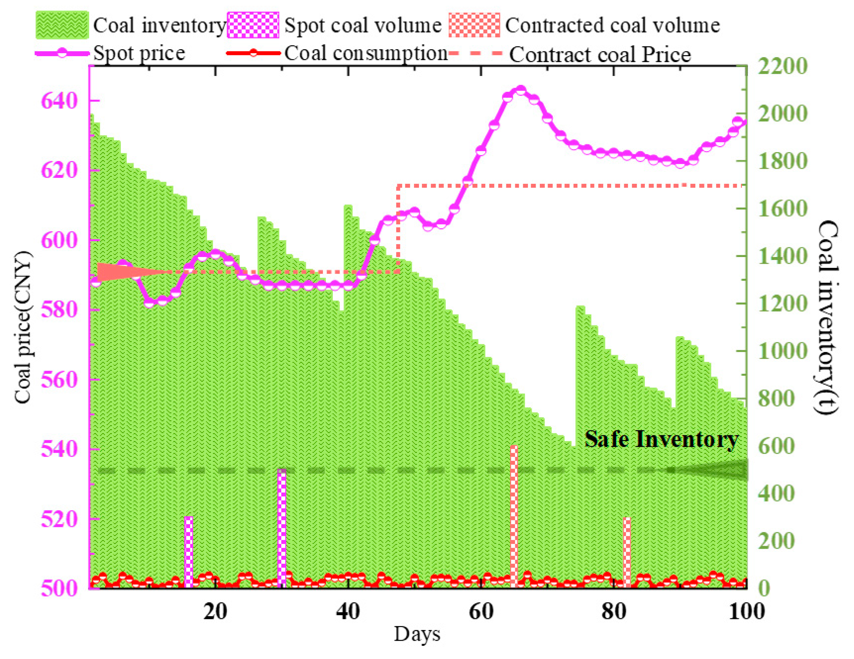
3.1.1. Description of Coal Procurement Timing Decisions

Coal procurement timing decision making is based on the short- and medium-term spot coal market information obtained from forecasting models. This includes making decisions on the timing and volume of spot coal purchases, as well as the rational scheduling of spot coal and contracted coal prices.

To facilitate description, the coal procurement indicator for the jth suppliers in the mth period is defined as the coal purchase flag bit $W_{m,j}^g$:

$$\left\{\begin{array}{l}if p_{m,j}^1<p_{m,j}^2,W_{m,j}^1=1,W_{m,j}^2=0\\ if p_{m,j}^1\ge p_{m,j}^2,W_{m,j}^1=0,W_{m,j}^2=1\end{array}\right.$$

(1)

where $W_{m,j}^1$ and $W_{m,j}^2$ are priority indicators for purchasing spot coal and contracted coal, respectively. $W_{m,j}^1$ = 1 indicates a priority for purchasing spot coal in period m, while $W_{m,j}^1$ = 0 indicates a priority for fulfilling long-term contract coal; $p_{m,j}^1$ and $p_{m,j}^2$ represent the predicted prices of spot coal and long-term contract coal, respectively, for the jth suppliers in period m.

3.1.2. Objective Function

In order to control the total cost of power generation in coal power plants, we adopted the cost of coal purchase decisions and inventory cost to characterize the total cost of power generation in coal power generation enterprises, assuming the existence of M coal supply vendors and N types of coal (according to the calorific value of the M suppliers, which are divided into N types) and then the total cost of power generation in the coal power generation enterprises. The total cost can be expressed as follows:

$$\min Cost={\displaystyle \sum _{m=1}^T{\displaystyle \sum _{g=1}^2{\displaystyle \sum _{j=1}^M(p_{m,j}^g+\phi )x_{m,j}^g{W}_{m,j}^g+p_{foreign,m}{x}_{foreign,m}+{\displaystyle \sum _{i=1}^N{S}_{m,i}\theta }}}}$$

(2)

where $x_{m,j}^1$ (decision variable) represents the quantity of spot coal purchased from jth-type suppliers in cycle m; $x_{m,j}^2$ (decision variable) represents the quantity of contracted coal decomposed in jth-type suppliers in cycle m; x_foreign,m denotes the quantity of spot coal purchased from foreign suppliers; $p_{m,j}^1$ is the price of the jth type of spot coal suppliers in cycle m; $p_{m,j}^2$ is the price of the jth type of contracted coal suppliers in cycle m; p_foreign,m denotes the price of spot coal purchased from foreign suppliers; φ represents the average warehouse overhead; S_m,i is the inventory of coal type i in cycle m; and θ is the unit inventory cost.

3.1.3. Constraints

Coal power plants need to make coal purchase decisions based on actual supplier supply capacity, generation inventory capacity limits, and actual coal consumption during the cycle, i.e., they need to consider the following constraints: upper and lower limits on supplier supply, inventory limits on categorized coals, and capacity limits on total inventories.

(1)

Suppliers’ supply constraints

The amount of coal purchased by a power generation company should not exceed the upper limit of the coal supplier’s supply, and in order to ensure the contract performance rate, the amount of coal purchased should not be lower than the minimum supply of the coal suppliers:

$$x_{\min ,j}^g\le x_{m,j}^g\le x_{\max ,j}^g$$

(3)

where for the jth type of coal supplier, $x_{\min ,j}^g$ is the minimum supply of coal suppliers, and $x_{\max ,j}^g$ is the upper limit of suppliers’ supply.

Some countries may have requirements for the proportion of coal purchased domestically and abroad: the amount of coal purchased from domestic and foreign sources needs to be in the proportion required by the industry.

$$\frac{{\displaystyle \sum _{m=1}^T{\displaystyle \sum _{g=1}^2{\displaystyle \sum _{j=1}^M{x}_{m,j}^g}}}}{{\displaystyle \sum _{m=1}^T{x}_{foreign,m}}}=r_m$$

(4)

where r_m denotes the ratio required by the industry standards in cycle m.

(2)

Categorized coal stockpile constraints

Coal purchased from various coal suppliers needs to be categorized according to its characteristics (calorific value, sulfur, etc.), and the amount of each type of coal needs to be categorized and stockpiled according to the subsequent blending situation to meet the needs of continuous production:

$$X_{m,i}={\displaystyle \sum _{g=1}^2{\displaystyle \sum _{j\in I_i}{x}_{m,j}^g{W}_{m,j}^g}}$$

(5)

$$S_{m,i}=S_{m-1,i}+X_{m,i}-C_m{\epsilon }_{m,i}$$

(6)

$$S_{\min ,i}\le S_{m,i}\le S_{\max ,i}$$

(7)

where for the ith type of coal in period m, I_i is the set of suppliers providing the ith type of coal, S_m−1,i is the stockpile of class i coal in the previous purchasing cycle, and X_m,i is the purchasing quantity of class i coal. S_m,i is the total stockpile quantity; C_m is the consumption of coal in the mth cycle, and ε_m,i is the blending ratio of coal of class i coal in the mth cycle, which is imported from the bottom layer model; S_min,i and S_max,i are the upper and lower limits of the stockpile of coal of class i, respectively.

(3)

Total inventory constraints

Subject to site constraints, the total inventory of all coals is required to satisfy the inventory constraint in Equation (8):

$$S_{\min }\le {\displaystyle \sum _{i=1}^N{S}_{m,i}}\le S_{\max }$$

(8)

where S_min and S_max represent the lower and upper limits of the total inventory of the power plant, respectively.

3.1.4. Optimizing Decision Variables

Considering the coal supply quantity of each coal supplier, the optimal spot coal price and contracted price, and the optimization objective of minimizing the total cost of coal purchase and inventory, the following decision variables are solved and substituted into the optimization model of blending ratio: $x_{m,j}^1$, the quantity of spot coal purchased from the jth supplier; $x_{m,j}^2$, the quantity of contracted coal purchased from the jth supplier in period m.

3.2. The Blending Ratio Decision Optimization Layer

The total electricity generation of power enterprises is typically determined through bidding or directives from the dispatch department. To focus on the dynamic coupling relationship between market coal price uncertainty and enterprise electricity production decisions, this study does not consider the participation of electricity generation in market competition. Instead, it only considers a scenario where the electricity generation quantity is given by the dispatch department for research purposes.

3.2.1. Objective Function

Considering the impact of the blending ratio on the coal purchase and inventory cost of coal power plants, assuming ε_m,i is the blending ratio of coal type i in cycle m, the unit blending cost in cycle m is $p_m^{unit}$, which determines the fuel blending unit price of power generation enterprises [24]. The optimization model of the coal-blending ratio takes the lowest unit blending price $p_m^{unit}$ in each cycle as the objective function:

$$\min p_m^{unit}=\frac{1}{F_m}{\displaystyle \sum _{i=1}^N{\epsilon }_{m,i}{X}_{m,i}(p_{m,i}+\phi +\theta )\frac{Q_{net}^{*}}{Q_{net,i}}}$$

(9)

where F_m denotes the electricity generation quantity in period m, N is the number of coal types, i denotes the coal type, ε_m,i is the blending ratio of coal type i in the mth cycle, X_m,i is the purchasing quantity of coal type i in the mth cycle, $p_{m,i}$ represents the average unit price of coal purchased in type i, φ represents the average stockpile management cost, θ is the unit stockpile cost, $Q_{net}^{*}$ is the calorific value of the standard coal (7000 kcal), and Q_net,i is the calorific value of the common coal.

In this paper, it is assumed that the power generation of a coal power company comes from the dispatch organization, which forecasts the load as well as the output from sustainable energy sources, such as wind and solar, in order to determine the power generation of a thermal power plant. Weibull theory and photovoltaic (PV) output curves have been widely used to model the typical output of a new energy source.

The wind speed satisfies the Weibull distribution, which is modeled as follows:

$$f(v)=\left(\frac{k}{c}\right){\left(\frac{v}{c}\right)}^{k-1}\exp \left[-{\left(\frac{v}{c}\right)}^k\right]$$

(10)

where c and k refer to the scale parameter and shape parameter of the Weibull distribution function, respectively; v is the wind speed in the actual environment, which is forecasted by the meteorological department before the month. The output power P_WT of the wind turbine can be expressed as follows:

$$P_{WT}=\left\{\begin{array}{l}0,v<v_{ci} or v\ge v_{co}\\ P_{WT}^N\frac{v-v_{in}}{v_N-v_{ci}},v_{ci}\le v<v_N\\ P_{WT}^N,v_N\le v<v_{co}\end{array}\right.$$

(11)

where v (m/s) is the actual wind speed; v_ci, v_co, and v_N are the cut-in wind speed, cut-out wind speed, and rated wind speed, respectively; P_WT is the rated power of the wind turbine.

$$P_{PV}=P_{stc}\frac{G_{AC}}{G_{stc}}\left[1+k(T_c-T_r)\right]$$

(12)

where G_stc and G_AC (kW/m²) represent the solar radiation intensity in the standard condition and the actual condition, respectively; P_PV and P_stc (kW) represent the actual output power of PV and the maximum output power of PV under the standard test environment (G = 1000 W/m², T_r = 250 °C), respectively; k is the temperature coefficient of the PV’s power, which is taken as −0.44%; T_c and T_r (°C) are the PV cell temperature and reference temperature, respectively.

The dispatch department forecasts the month-ahead PV generation, wind generation, and total load from meteorological data and also calculates the month-ahead generation schedule F_m allocated to the coal power companies.

$$F_m=loa{d}_m-F_{WT}-F_{PV}$$

(13)

where load_m denotes the total load for period m, F_WT represents the wind power generation, and F_PV is the photovoltaic power generation.

3.2.2. Constraints

(1)

Heating constraints

Blending is carried out in accordance with a certain ratio of coal consumption, and the total heat generated needs to meet the requirements of the production and power generation plan:

$$C_m^s=\frac{F_m{g}_m}{1-{\eta }_g}$$

(14)

$$C_m^s{Q}_{net}^{*}\le {\displaystyle \sum _{i=1}^N{C}_m{\epsilon }_{m,i}{Q}_{net,i}\beta }$$

(15)

where $C_m^s$ is the standard coal consumption in the mth cycle, C_m is the coal consumption in the mth cycle, g_m is the standard coal consumption per unit of power generation in the mth cycle, η_g is the self-consumption rate of power generation, and β is the coal efficiency of the boiler.

(2)

Inventory consumption constraints

The consumption of each type of coal needs to be adjusted according to the stockpile and must not exceed the upper limit of the classified coal stockpile.

$$0\le C_m{\epsilon }_{m,i}\le S_{m-1,i}+X_{m.i}$$

(16)

(3)

Production target constraints

In order to ensure production safety and reduce environmental maintenance costs, coal-blending production needs to meet the boiler blending safety production conditions:

$$L_{\min }\le {\displaystyle \sum _{i=1}^N{\epsilon }_{m,i}{L}_i}\le L_{\max }$$

(17)

$$V_{\min }\le {\displaystyle \sum _{i=1}^N{\epsilon }_{m,i}{V}_i}\le V_{\max }$$

(18)

$$T_{\min }\le {\displaystyle \sum _{i=1}^N{\epsilon }_{m,i}{T}_i}\le T_{\max }$$

(19)

where L_min and L_max are the upper and lower limits of average sulfur content of blended coal blending, and L_i is the sulfur content of coal type i; V_min and V_max are the upper and lower limits of dry ashless volatile matter of blended coal blending, and V_i is the dry ashless volatile matter of coal type i; T_min and T_max are the upper and lower limits of the melting point of blended coal blending, and T_i is the melting point of blended coal blending of coal type i. The average sulfur content of blended coal blending is the lower limit of the average sulfur content of blended coal blending.

3.2.3. Optimizing Decision Variables

Considering the optimization objective of minimizing the cost of blending, the lowest incoming unit of the cycle, the decision variables, and related variables of this section are solved and passed to the upper-layer model: the decision variable is the percentage of coal blending of type i in the mth cycle ε_m,I, and the pass-through variable is the amount of coal of type i used in the mth cycle C_m,i.

3.3. The Solution Strategy of the Dual-Layer Model

In the above model, the upper-layer coal purchase timing decision model is a linear model whose classification inventory constraints are governed by the optimization results of the bottom-layer blending ratio optimization model. The objective function of the bottom-layer model contains bilinear terms, which are indirectly determined by the solution result of the upper-layer model. The upper- and bottom-layer models interact with each other, so the established model belongs to the double-layer nonlinear optimization model; this type of dual-layer model has been proven to be a nondeterministic polynomial (NP) problem [25], and common solvers are difficult to solve it directly.

However, there are more mature solution methods available for the study of two-layer nonlinear optimization models, and these methods can be generally classified into two categories [26]:

(1)

Dual-layer planning is transformed into a single-layer model using the variational inequality method or the K-T (Karush–Kuhn–Tucker, KKT) method and then linearly transformed.

(2)

Iterative methods based on numerical or non-numerical optimization continuously reduce the gap between the locally better solution and the globally optimal solution through hierarchical solving and multiple global iterations.

The model proposed in this paper is a double-layer nonlinear optimization model. In order to ensure the solution accuracy using category (1), and to respond to the change in the total cost of the coal power plant, the upper-layer model is selected as the main model. First, the bilinear term of the lower-layer objective function is relaxed based on the McCormick envelope. Secondly, the lower-layer model is converted to the nonlinear constraints of the upper-layer model using the KKT method and linearized based on the large M method. Finally, the solution is found using the Gurobi solver.

3.3.1. McCormick Envelope-Based Bilinear Term Relaxation

The lower-layer model’s objective function is a bilinear nonconvex model, which does not satisfy the KKT transformation requirement. The relaxation of the bilinear terms is considered, which is classically carried out using the McCormick envelope [27]. For any bilinear term in the objective function of the lower-layer doping ratio optimization model, the variable w_m,i is used to replace it, and the corresponding relaxation constraints are added at the same time. The converted objective function and constraints are as follows:

$$\begin{array}{cc}\hfill & min{p}_m^{unit}=\frac{1}{F_m}{\displaystyle \sum _{i=1}^N}{w}_{m,i}(p_{m,i}+\phi +\theta )\frac{Q_{net}^{*}}{Q_{net,i}}\hfill \\ \hfill & s.t.\left\{\begin{array}{c}{w}_{m,i}\ge ({\epsilon }_{m,i}^{min}{X}_{m,i}+{\epsilon }_{m,i}{X}_{m,i}^{min}-{\epsilon }_{m,i}^{min}{X}_{m,i}^{min})\hfill \\ w_{m,i}\ge ({\epsilon }_{m,i}^{max}{X}_{m,i}+{\epsilon }_{m,i}{X}_{m,i}^{max}-{\epsilon }_{m,i}^{max}{X}_{m,i}^{max})\hfill \\ w_{m,i}\le ({\epsilon }_{m,i}^{max}{X}_{m,i}+{\epsilon }_{m,i}{X}_{m,i}^{min}-{\epsilon }_{m,i}^{max}{X}_{m,i}^{min})\hfill \\ w_{m,i}\le ({\epsilon }_{m,i}^{min}{X}_{m,i}+{\epsilon }_{m,i}{X}_{m,i}^{max}-{\epsilon }_{m,i}^{min}{X}_{m,i}^{max})\hfill \\ \mathrm{E}\mathrm{q}\mathrm{u}\mathrm{a}\mathrm{t}\mathrm{i}\mathrm{o}\mathrm{n}\mathrm{s}\left(9\right)–\left(14\right)\hfill \end{array}\right.\hfill \end{array}$$

(20)

At this point, the lower-layer doping ratio optimization model is reconstructed as a convex model after linear relaxation with the McCormick envelope [28], so the model transformation condition based on the K-T method is sufficient, i.e., the doping ratio optimization model under this method can achieve its minimum value. Additionally, the error introduced by the McCormick envelope can be adjusted to the newly introduced relaxation constraints based on the subsequent optimization results.

3.3.2. Model Equivalence Based on Karush–Kuhn–Tucker

The bottom-layer model’s objective function and its constraints are convex after linear relaxation by the McCormick envelope and satisfy Slater’s condition, which meets the condition of single-layer model transformation for the two-layer model using the KKT optimality condition. The Lagrangian function of the lower-layer model is constructed as shown in Equation (21).

$$\begin{array}{c}\hfill L(w_{m,i},{\epsilon }_{m,i},X_{m,i},\overrightarrow{\lambda },\overrightarrow{\mu })= {\displaystyle \sum _{k=1}^n{\mu }_{k}g(w_{m,i},{\epsilon }_{m,i},X_{m,i})}\\ \hfill +p_m^{unit} + {\displaystyle \sum _{k=1}^l{\lambda }_{k}h(w_{m,i},{\epsilon }_{m,i},X_{m,i})}\end{array}$$

(21)

where λ and μ are the Lagrange multiplier vector and the KKT multiplier vector, respectively; $p_m^{unit}$ is the lower-layer model’s objective function; h(w_m,i, ε_m,i) is the equality constraint; and g(w_m,i, ε_m,i) is the inequality constraint.

When the objective function of the lower-layer model obtains the minimum value, the lower-layer model satisfies the KKT optimization condition, and the Lagrangian function has a partial derivation of 0 with respect to the included variables, as shown in Equation (22).

$$\frac{\partial L}{\partial (w_{m,i},{\epsilon }_{m,i},X_{m,i})}=0$$

(22)

where the inequality constraints have a complementary dyadic relationship with each multiplier; the complementary relaxation condition is shown in Equation (23).

$$0\le {\mu }_k\perp g(w_{m,i},{\epsilon }_{m,i},X_{m,i})\le 0,k=1,2,\dots ,n$$

(23)

where n is the number of inequality constraints.

Obviously, the product term of the Lagrange multiplier of the inequality and inequality constraint is nonlinear, and the nonlinear term continues to be eliminated with the large M method. The specific steps are shown in Equation (24).

$$\left\{\begin{array}{l}0\le {\mu }_k\perp g(w_{m,i},{\epsilon }_{m,i},X_{m,i})\le 0,k=1,2,\dots ,n\\ {\mu }_k\le z_{k}M\\ -g_k(w_{m,i},{\epsilon }_{m,i},X_{m,i})\le (1-z_k)M\end{array}\right.$$

(24)

where k is the inequality constraint labeling, z_k is a 0–1 variable, and M is a sufficiently large number.

So far, based on the joint Equations (2)–(7) and Equations (22)–(24), the dual-layer dynamic collaborative decision optimization model constructed in this paper is equivalent to a single-layer integer linear programming model, which is solved based on MATLAB (2022b) by invoking the Gurobi solver (10.0).

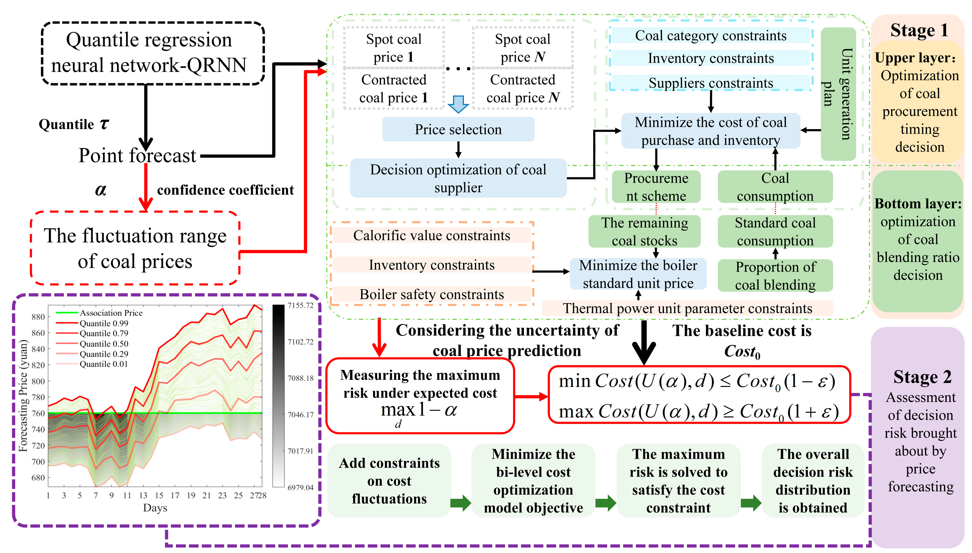
4. Decision Risk Measurement Method Based on QDD-IGDT

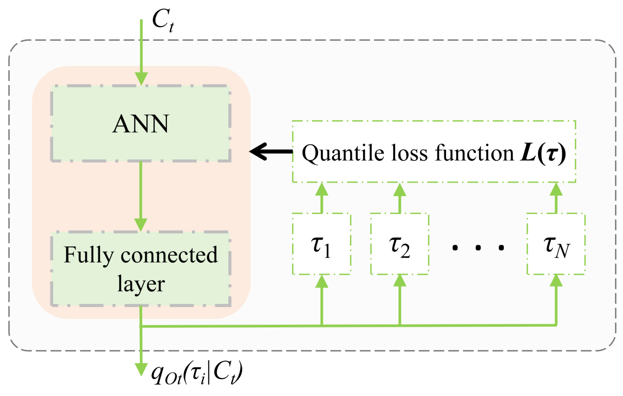
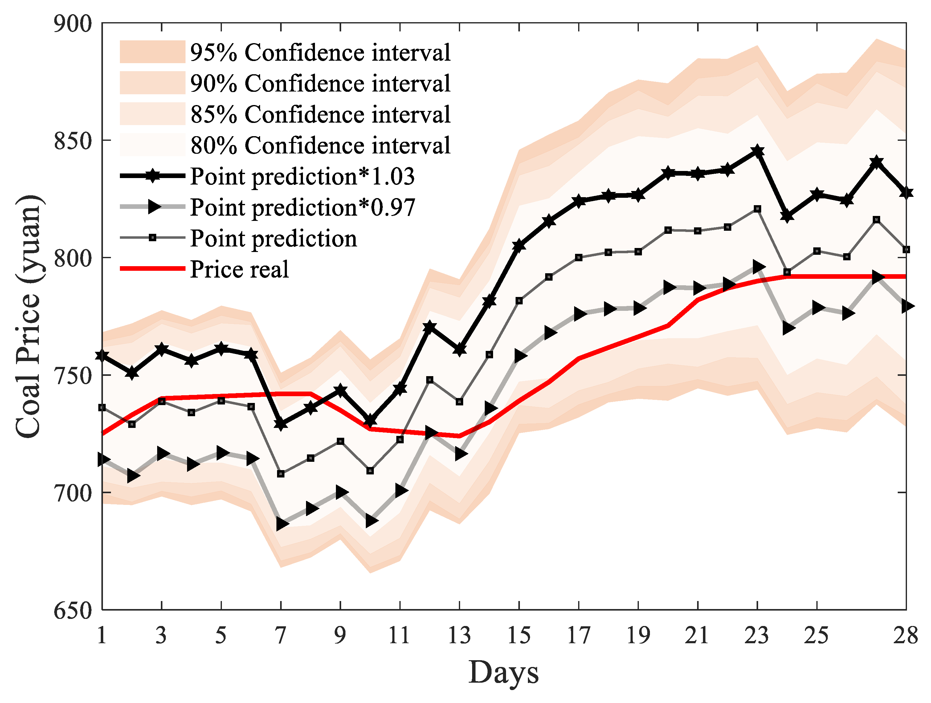
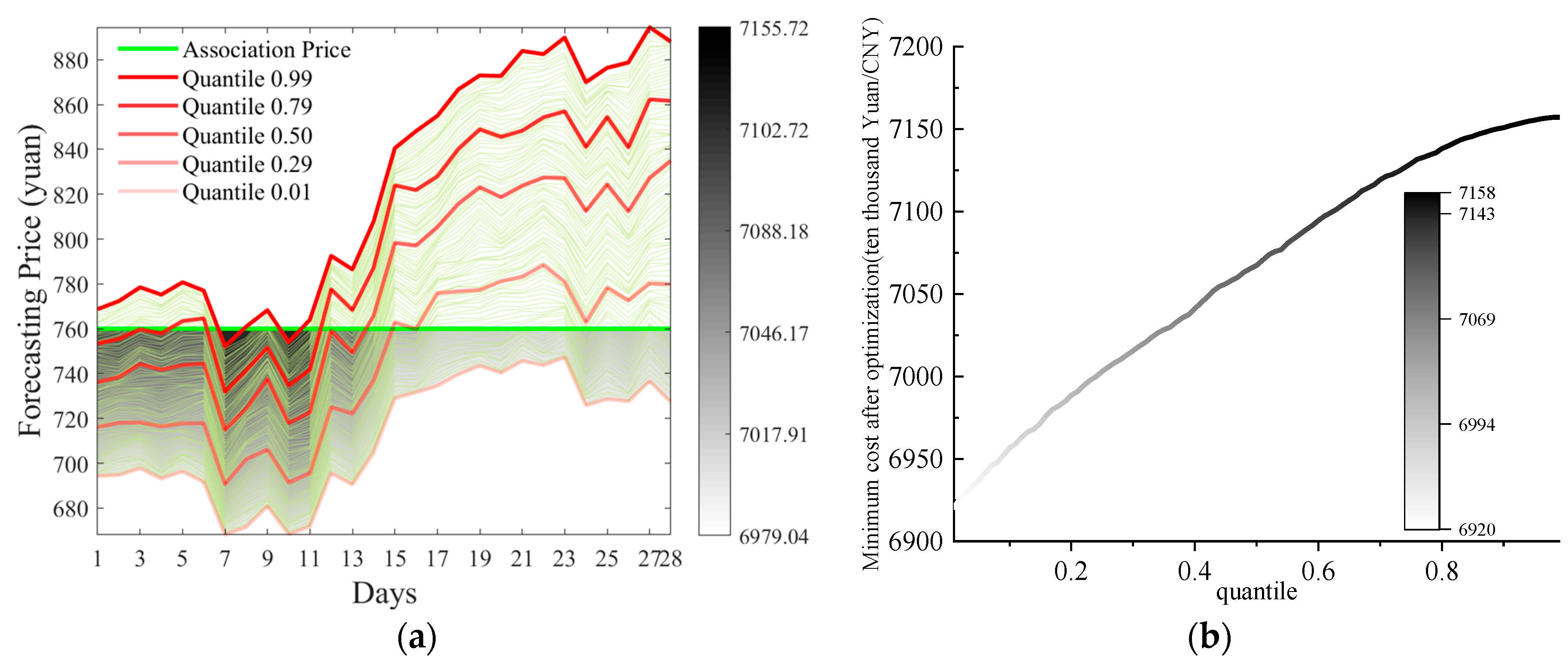
4.1. Construction of a Coal Price Quantile Dataset Based on QRNN

In this paper, we construct a coal price quantile dataset based on a quantile regression neural network (QRNN) model to predict the coal price range. The structural principle is shown in Figure 3. c_t and q_Ot (τ_i|C_t) are the input features at time series t and the output of the network when the quantile is τ_i, respectively.

The prediction interval I_α with confidence level α can be expressed as follows:

$$I_{\alpha }=[q_{{\tau }_d},q_{{\tau }_u}]$$

(25)

where τ_d and τ_u are the lower and upper quartiles, respectively, and q_τ is the QRNN output when the loss function is defined as L(τ), and L(τ) is defined as follows:

$$L(\tau )=\frac{1}{N_L}{\displaystyle \sum _{t=1}^N{\rho }_{\tau }(q_{\tau }(t)-q(t))}+\lambda {\displaystyle \sum _{t=1}^m{W}_b^2}$$

(26)

where N_L is the number of input variables, ρ_τ is the pinball loss function, q_τ is the model output value, q is the actual value when the model is trained, λ is the hyperparameter, and W_b is the target training parameter matrix.

In order to meet the needs of the coal cost optimization module, we selected the data regarding coal production, imported coal quantity, and port cargo volume as input features based on Pearson’s coefficient and Granger’s calibration method, set different confidence levels α, and realized the short- and medium-term interval prediction of spot coal price based on the QRNN model with day as granularity and month as cycle.

In Figure 4, the black and gray lines represent the traditional use of point prediction and active panning to construct the coal price uncertainty domain over any time period of the information gap. This approach fails to capture the characteristic of increasing uncertainty in coal prices with the increasing forecast time scale. In contrast, for the coal price quantile dataset, as the confidence level and forecast time scale increase, the information gap between upper and lower intervals widens at any given time period. This provides additional information for decision makers during the process of decision risk measurement.

4.2. Traditional Information-Gap Theory

The classical model of traditional IGDT is as follows:

$${\alpha }_f(d,r_c)\triangleq \max \{\alpha :r_c\le \underset{u\in U(\alpha ,\tilde{u})}{\min }R(d,u)\}$$

(27)

where α_f is the robustness function with the value of the uncertainty factor α between [0, 1], which is determined by the coal purchase and blending decision scheme d(W, x, ε) and the cost threshold r_c. R is the reward function, which is set to be the inverse of the cost of the coal power plant 1/Cost, and the reward function is affected by the uncertainty quantity u. U in Equation (27) is defined as the set of all the uncertainty quantities u.

The measurement of the uncertainty factor u is typically conducted using a fractional error model to create an extended interval, as shown in Equation (28).

$$U(\alpha ,\tilde{u})=\left\{u:\left|\frac{u-\tilde{u}}{\tilde{u}}\right|\le re\times \alpha \right\}$$

(28)

where re is a vector of folding coefficients and is further expanded as follows:

$$(1-re\times \alpha )\tilde{u}\le u\le (1+re\times \alpha )\tilde{u}$$

(29)

4.3. Risk Metrics Based on Quantile Data-Driven Information-Gap Theory

The traditional IGDT portrays the fluctuation intervals of uncertain parameters by assigning weights re, which is highly subjective, and the uncertainty measure results are only interpreted as the fluctuation amplitude of uncertain parameters, which is poorly interpretable and less informative and cannot comprehensively guide the coal power plant in the optimization task of cost decision making.

In this paper, we determine the IGDT using a binned dataset by defining the uncertainty domain U(α); α is the confidence level, U(α) is the coal price uncertainty domain, and I_α is defined as the prediction interval created when the confidence level is α. Q_pre is the QRNN output when the loss function is defined as L(τ).

$$\left\{\begin{array}{l}0\le \alpha \le 1\\ U(\alpha )=I_{\alpha }=\{u:q({\tau }_d)\le u\le q({\tau }_u)\}\\ q(\tau )=Q_{pre}:L(\tau )=+\lambda {\displaystyle \sum _{t=1}^m{W}_b^2}\\ \hspace{1em}\hspace{1em}\hspace{1em}\hspace{1em}\hspace{1em}+\frac{1}{N}{\displaystyle \sum _{t=1}^N{\rho }_{\tau }(q_{\tau }(t)-q(t))}\end{array}\right.$$

(30)

In order to reasonably measure the fluctuation of coal power cost affected by the uncertainty of market coal price and to improve the interpretability of the uncertainty measurement results, we define the optimization objective α as the QRNN confidence level and add the constraint of the envelope interval of the expected cost to obtain the confidence level under each expected cost interval, so as to establish the quantile data-driven IGDT decision-making risk measurement model (QDD-IGDT), which can be described as follows:

$$\begin{array}{l}\underset{d}{\max }1-\alpha \\ s.t.\left\{\begin{array}{l}0\le \alpha \le 1\\ U(\alpha )=I_{\alpha }=\{u:q({\tau }_d)\le u\le q({\tau }_u)\}\\ q(\tau )=Q_{pre}:L(\tau )\\ \min Cost(U(\alpha ),d)\le Cos{t}_0(1-\epsilon )\\ \max Cost(U(\alpha ),d)\ge Cos{t}_0(1+\epsilon )\\ s.t.Cost\end{array}\right.\end{array}$$

(31)

where α is the confidence level; 1 − α is the risk level; and minCost(U(α),d) and maxCost(U(α),d) are the minimum and maximum costs of the dual-layer cost optimization model, respectively. Setting Cost₀ as the baseline cost represents the optimization result of the cost optimization model when the input spot coal price represents the cost volatility, which is determined by the decision maker.

The above risk metrics are determined by incorporating the QRNN model into the coal price quantile dataset in order to eliminate the subjectivity of the traditional IGDT method in constructing the coal price uncertainty domain. Second, the decision risk metric model of quantile data-driven IGDT is established by optimizing the maximum risk level of the cost interval constraint. Finally, the decision risk is optimized to reach the expected cost interval to explore the risk in the decision maker’s decision to obtain a certain cost fluctuation interval in the context of coal market uncertainty and to realize the uncertainty risk metric of the coal power cost production decision.

5. Results and Discussion

A coal-fired power plant with an installed capacity of 2 × 660 MW was used as a research object to co-optimize coal purchase and production decisions. The standard coal consumption characteristic curve of each unit is shown in Figure 5. The generation schedule of thermal power, PV power, wind power, and total power are shown in Figure 6. The details of the inbound tender list provided by optionally contracted coal suppliers are shown in Figure 7. The results of the prediction of the short- and medium-term price ranges of CCI5500 spot coal are shown in Figure 7. The average warehouse management cost was set at 4 CNY/ton, and the average unit inventory cost is 20 CNY/ton; the detailed information of the suppliers for each coal type is shown in

Table 1. Characteristic information of each type of coal.

Coal Class Number	Calorific Value (kcal)	Sulfur (%)	Gray Melting Point
A-001	5500	0.6	1500
A-002	5500	0.6	1500
A-003	5500	0.6	1500
A-004	5500	0.6	1500
A-005	5500	0.6	1200
A-006	5000	0.6	1200
A-007	5000	0.6	1200
A-008	5000	0.6	1200
A-009	5000	0.6	1500
A-010	5000	0.6	1500
A-011	5250	1.5	1200
spot coal	5000	0.6	1200

.

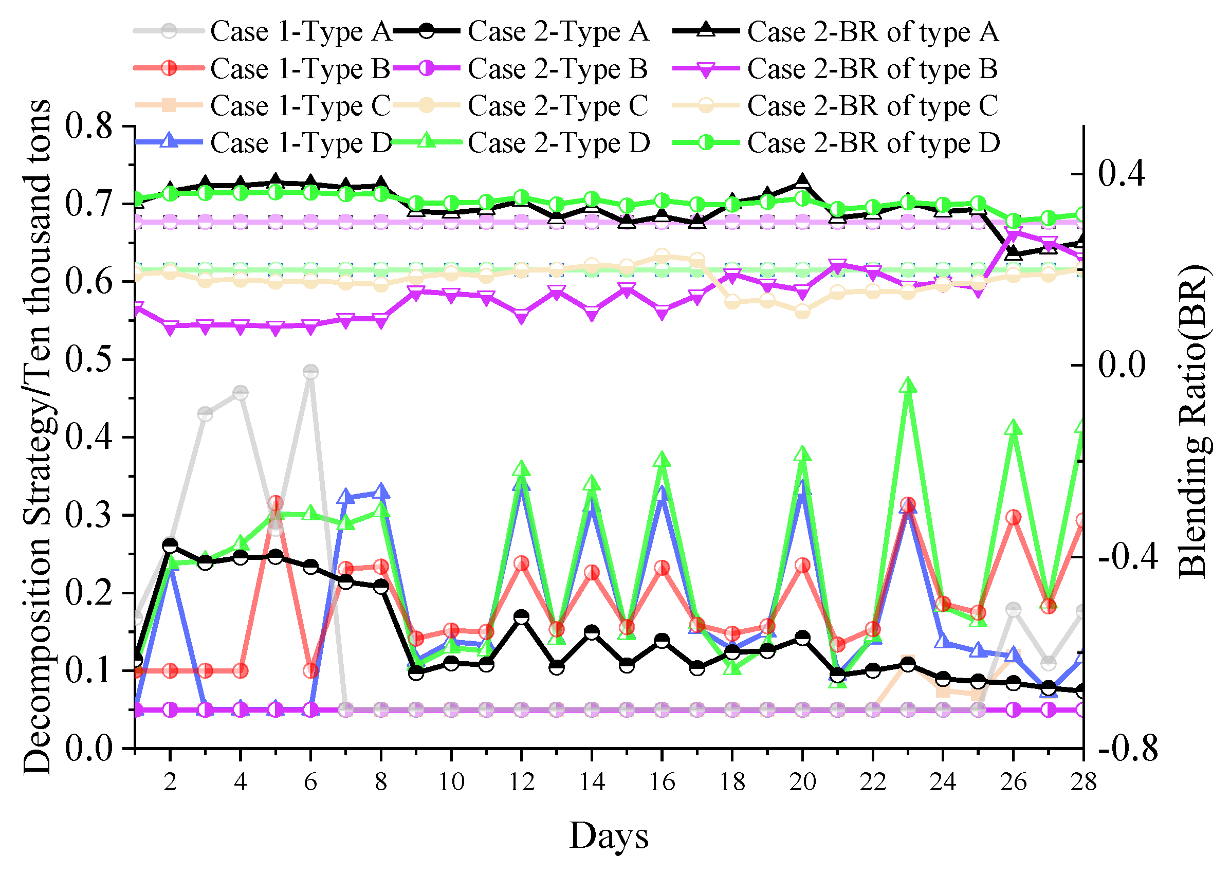
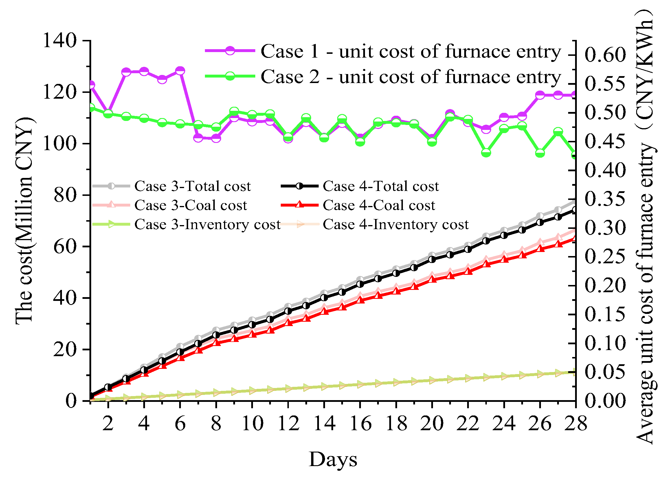
5.1. Utility Analysis of the Dual-Layer Optimization Model for Electricity Generation Side Market Decisions

Firstly, considering only the long-term contract coal ($W_{m,j}^1$ = 0), two cases were designed to analyze the effectiveness of the proposed dual-layer model and the solution method. Case 1 involved solving the upper-layer coal procurement optimization model based on the Gurobi solver without considering the blending optimization layer; Case 2 considered the blending optimization layer and solving the dual-layer dynamic collaborative decision-making optimization model of power generation based on the KKT–McCormick–Gurobi method. The blending ratios of the four contracted coals in Case 1 were set to 0.3:0.3:0.2:0.2 [29]. The Case 2 model was transformed into a linear mixed-integer programming model after the McCormick envelope and KKT conditions, and the MATLAB-based Gurobi solver was called for solving.

Figure 8 shows the optimization results of the blending ratios and the comparison of coal purchasing decisions in Case 1 and Case 2. Coal types 1–4 represent coals with calorific values of 5500 kcal, 5000 kcal, 5250 kcal, and 3800 kcal, respectively. In Case 1, with a fixed blending ratio, coal purchases are mainly focused on type 2 and type 4 coals; in Case 2, coal purchases are mainly focused on lower-priced type 1 and type 4 coals. In Case 1, due to the lack of perception of the unit blending cost and the inability to adjust the blending ratio, a large number of lower-priced type 1 coals are purchased in the early stage to meet the safety stock requirements, as shown in Figure 8, and in the middle stage, after the type 2 coals bottom out, a large number of high-priced type 2 coals are decomposed to meet the demand for high consumption, resulting in a sharp increase in the cost of purchased coals due to the blending ratio remaining unchanged. In Case 2, a dynamic variation is generated in the blending ratio by sensing the unit blending cost, reducing the consumption of type 2 coal in the first and middle stages, and increasing the amount of lower-priced type 1 coal decomposed to meet the inventory and consumption requirements to bring about a reduction in cost.

Figure 9 shows the comparison of the unit blending cost and the total cost between Case 1 and Case 2, and

Table 2. Comparison of production cost indicators between case 1 and case2.

Norm	Cost of Inventory	Cost of Coals	Total Cost	Unit Cost
Unit	Million (CNY)	Million (CNY)	Million (CNY)	CNY
Case 1	11.20	66.58	77.78	0.4986
Case 2	11.20	63.20	74.39	0.4761

shows the comparison of the total cost and the inventory cost under each case. Firstly, as shown in Figure 9 and Table 2, the unit blending cost of Case 2 is lower than that of Case 1 most of the time, and its average value decreases from CNY 0.4986 to CNY 0.4761. The purchasing cost as well as the total cost are lower than those of Case 1 at all times. The coal purchase cost and the total cost are lower than Case 1 all the time, and from the above analysis, it can be seen that the coal purchase decision optimization ability of the power generation and production dual-layer dynamic collaborative decision optimization model is stronger. Secondly, the total cost of Case 2 is reduced from CNY 77.78 million to CNY 74.39 million compared with Case 1; the cost of coal purchase is CNY 63.20 million, which is CNY 0.34 million lower than that of Case 1. The other detailed indicators are shown in Table 2.

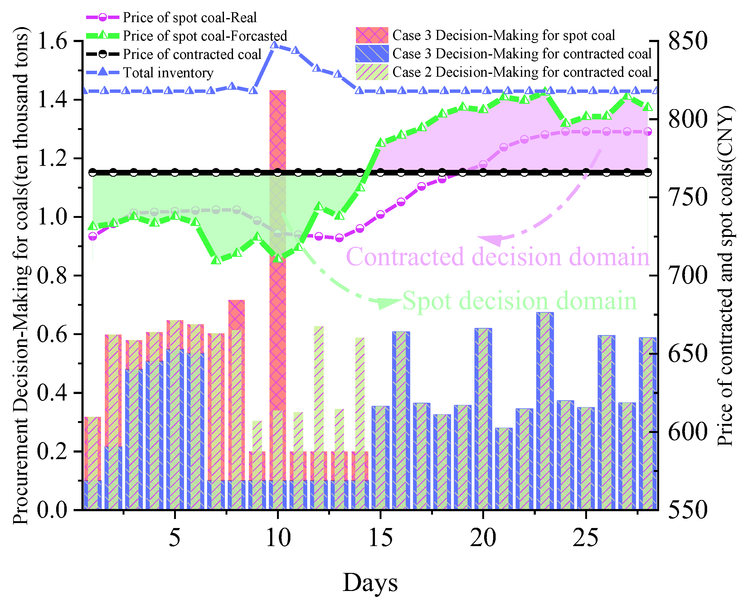
5.2. Quantitative Analysis of Dual-Layer Decision Optimization Model with Spot Coal and Long-Term Contract Coal Price Optimization

In order to investigate the cost optimization utility of the dual-layer dynamic decision-making optimization model of power generation and production with the optimization of the prices of spot coal and contracted coal, Case 2 in the previous section, namely the dual-layer decision-making optimization model of power generation and production without price optimization (only considering the decomposition of contracted coal), is used as the control group. Case 3, i.e., the dual-layer dynamic collaborative decision-making optimization model of power generation and production with the optimization of the prices of spot coal and contracted coal, is designed as the experimental group.

Figure 10 shows the optimization results of the coal purchase decisions for Case 2 and Case 3, and

Table 3. Comparison of production cost indicators between case 2 and case3.

Norm	Cost of Inventory	Cost of Coals	Total Cost	Unit Cost
Unit	Million (CNY)	Million (CNY)	Million (CNY)	CNY
Case 2	11.20	63.19	74.39	0.4761
Case 3	11.32	62.33	73.65	0.4704

shows the comparison of various types of indicators. The results show that the proposed model is able to further reduce the total cost of the power plant by CNY 0.745 million, or 1.0001%, compared with Case 2. Among them, the cost of coal purchase is reduced from CNY 63.19 million to CNY 62.33 million, and the inventory cost is increased from CNY 11.20 million to CNY 11.32 million. This is due to the fact that the proposed model is able to perceive the change in spot coal price and give up a certain inventory cost optimization space in order to allow for purchasing a large amount of spot coal when the spot coal price is low. As shown in Figure 10, on the 8th and 10th days, the forecast price of spot coal is lower than the price of contracted coal and at a low level, so the decision maker buys a large amount of spot coal to pull up the inventory and consumes a large amount of spot coal from the 11th to 14th days when the price of spot coal is relatively high, so as to realize “pulling up the inventory at a low price level, shifting to power generation at a high price level”, and optimizing the whole situation dynamically.

When the spot coal price is low, the decision maker purchases lower-priced spot coal to reduce power generation costs and increase profit margins. When the spot coal price is high, the decision maker mainly consumes the spot coal in the inventory and increases the breakdown of contracted coal to support the production demand of power plants. In the early stage of the coal purchase cycle, when the spot coal price is lower than the contracted coal price, the decision maker reduces the purchase cost by replacing part of the contracted coal with spot coal. Later, the spot coal price gradually increases, and coal consumption is mainly based on the remaining spot coal stockpile accumulated in the earlier stage and the existing contracted coal break-up volume.

From Table 3, it can be seen that the total cost of Case 3 decreases from CNY 74.39 million to CNY 73.65 million, which reduces the generation cost of the power plant, while the unit cost (the average value of the unit blending cost) becomes smaller than that of Case 2 due to a small increase in the cost of inventories and a significant decrease in the cost of purchased coal.

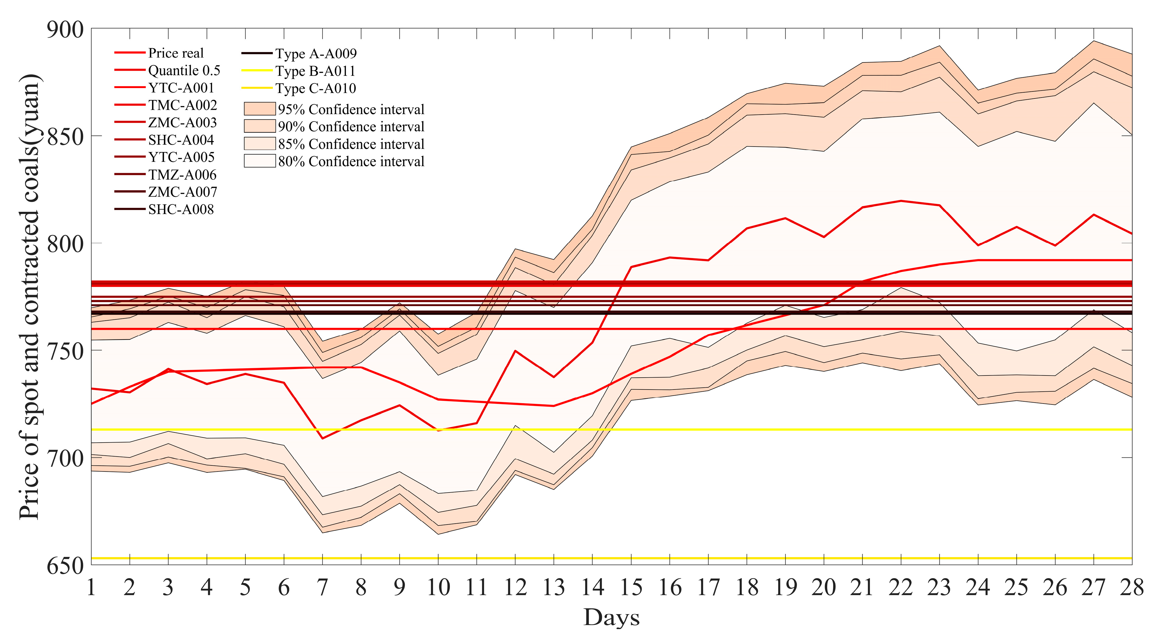
5.3. Market Decision-Making Risk Measurement Based on QDD-IGDT

Decision makers who make decisions based on forecasted coal prices alone will be at risk, and coal power plants usually need to further measure spot coal prices based on their forecasts in order to know the impact of the uncertainty brought about by the introduction of forecasted coal prices on the optimization of decision making as well as on cost changes.

The cost optimization results of Case 3 are used as the baseline Cost₀, and different expected cost volatilities ε are set to obtain the risk measures of decision uncertainty for coal power plants under different risk attitudes.

Table 4. Measures of uncertainty and its total cost under different cost intervals.

Cost Fluctuations ε%	Cost Range (CNY million)	min α%	max 1 − α%
0.1	[70.60, 70.74]	53	47
0.3	[70.46, 70.88]	58	42
0.5	[70.32, 71.02]	64	36
0.7	[70.17, 71.16]	70	30
0.9	[70.03, 71.30]	75	25
1.1	[69.89, 71.45]	85	15
1.215	[69.79, 71.55]	95	5

shows the minimum confidence level and the maximum decision risk needed to satisfy different expected cost volatilities. Table 4 shows that as the width of the decision maker’s expected cost range increases, the minimum confidence level that needs to be achieved increases, indicating that the decision maker needs to bear the maximum risk to make the decision more robust. Taking the cost range of CNY [70.17, 71.16] million as an example, the fluctuation range of spot coal prices needs to meet the 70% confidence level. At this time, the decision maker needs to bear 30% of the decision-making risk in order to achieve the expected cost range. When the expected cost volatility rises to 1.215%, the confidence level reaches 95%, which indicates that the introduction of coal price forecasting to assist the decision-making process results in a very low level of decision-making risk, and the cost changes basically do not overflow the expected cost range.

Figure 11a shows a collection of spot coal price prediction curves generated by taking different quartiles, and the lower half of the part surrounded by the quartile coal price curves and the contracted coal price curves is the spot decision domain. As the quantile increases, the depth of the spot decision domain deepens, and the minimum cost optimization results keep increasing, corresponding to Figure 11a. The color depth of the region between the curves becomes deeper as the cost Cost(q(τ_i), d) increases. This is due to the fact that the decision domain of spot coal shrinks as the quantile rises, the spot coal decision space that can be provided to the decision maker decreases, and the cost optimization space gradually decreases.

Figure 11b shows the cost optimization result Cost(q(τ), d) change after inputting the dual-layer decision optimization model by taking the quartile 1% to the quartile 99% to get different spot coal price forecast results. As can be seen from Figure 11b, with the gradual increase in the quantile, the optimized minimum cost rises, the color of the curve deepens, and the first half of the curve is close to linear, while the second half tends to be smooth. This is due to the fact that in the second half of the curve, the quantile is larger, most of the coal price prediction curve is higher than the contracted coal price, the decision domain of spot coal purchase is sharply narrowed, and the space for cost optimization is basically reduced.

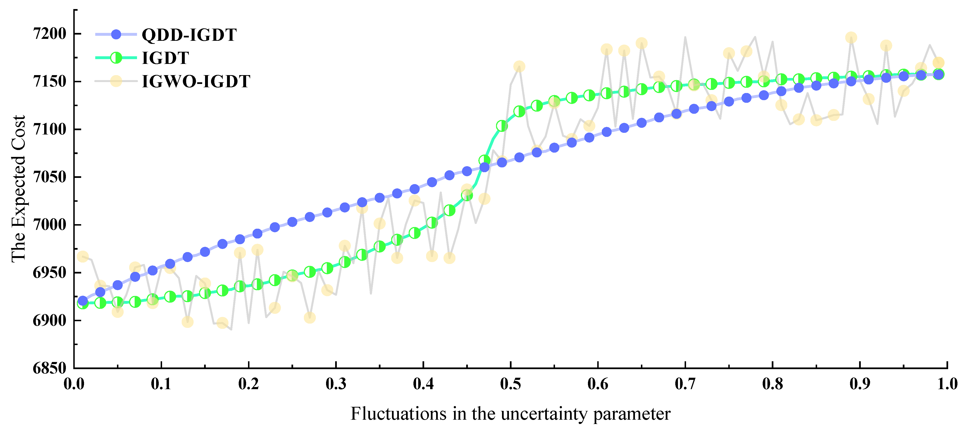
5.4. Comparison of the Results among IGDT, IGWO-IGDT, and QDD-IGDT

For the QDD-IGDT method proposed in this paper, we compare the QDD-IGDT method with the original IGDT and the IGWO-IGDT (improved gray wolf optimization IGDT, IGWO-IGDT). The above algorithms are compared with the method proposed in this paper to demonstrate the effectiveness and advancement of the proposed method.

As shown in Figure 12, the main fluctuation bands of the expected cost curve of the traditional IGDT method are concentrated in the middle part of the curve, while they are smoother on the left and right sides of the expected cost curve, which leads to the difficulty of the expected cost curve to reflect the decision-making risk under the large fluctuation of the cost. This is because when seeking risks and avoiding risks, the fluctuation intervals of uncertain variables constructed with the traditional IGDT method are simple and cannot measure the decision-making risk of decision makers in complex scenarios. The IGWO-IGDT-based method has the ability to escape from local optimums due to the use of swarm algorithms for model solving, which is also limited by the IGDT method, and it is difficult to provide a good decision horizon on the right side of the curve.

Compared with the traditional IGDT method and the IGWO-IGDT method, the method proposed in this paper can provide a good decision horizon for the decision maker because the fluctuation intervals of the uncertainty variables are constructed accurately, the cost changes and decision risks caused by the fluctuations in the coal market are calculated accurately, and the cost changes are more obvious in the whole fluctuation range of the uncertainty variables. In conclusion, the fluctuation interval of uncertain variables constructed with the method proposed in this paper is more accurate, and it is more efficient and robust than the traditional IGDT method and IGWO-IGDT method, which provides a broader decision-making horizon for coal power enterprises.

6. Conclusions

The aim of this study was to investigate the production decision optimization method of power generation enterprises in the context of the low willingness of coal power enterprises to generate electricity and uncertainty in the coal market. Therefore, this paper focused on the entire process of thermal power generation and introduced the quantile data-driven information-gap decision theory to describe the risk of uncertainty. Through the arithmetic simulation of the actual production data of a power generation enterprise, the following conclusions are drawn:

(1)

We conducted cost optimization through the establishment of a dynamic coordinated decision optimization model for electricity production with the optimization of spot coal and long-term contract coal prices. We compared its cost optimization capability with a single-tier coal procurement optimization model that did not consider blending optimization and with a two-tier decision optimization model that did not consider coal market prices. The proposed model can effectively improve the long-term decision-making cost optimization ability of power generation enterprises, and the production cost can be significantly reduced, realizing the “pulling up inventory at low a price level, shifting to power generation at a high price level”.

(2)

By introducing the quantile data-driven information-gap decision theory and addressing the limitations of the traditional IGDT method, we introduced the quantile range constraints and proposed the QDD-IGDT method to measure the risk of uncertainty in the decision-making process in the coal market, in order to explore the impact of market coal price uncertainty on the cost optimization of coal power plants. The expected cost fluctuation coefficient was set to obtain the minimum confidence level and the maximum risk assumption under different demands, which provides a less subjective, more robust, and broader decision-making risk metric for the cost optimization of coal power plants.

(3)

Our research results show that the proposed methodology can reduce the cost of power generators that include coal-fired units in the context of the continued development of renewable energy while coal units are being phased out. The two-tier cost optimization methodology proposed in this paper is applicable to power generation aggregators that include sustainable energy sources and thermal units by reducing the marginal cost of the generation of coal units in order to gain more profit in the electricity market and increasing the investment in renewable energy sources in order to increase the welfare of the society.

References

1. Guo, J.R.; Xiang, Y.; Wu, J.J. Low-carbon Optimal Scheduling of Integrated Electricity-gas Energy Systems Considering CCUS-P2G Technology and Risk of Carbon Mark. Proc. CSEE 2023, 43, 1290–1303. [Google Scholar]
2. Wang, B.; Qiu, Z.; Cong, X.; Zheng, Y.; Feng, S. Mechanism Analysis of Flexible Resources’ Marginal Price in New Energy Grid Based on Two-stage Stochastic Optimization Modeling. Proc. CSEE 2021, 41, 1348–1359. [Google Scholar]
3. Tiedemann, S.; Müller-Hansen, F. Auctions to phase out coal power: Lessons learned from Germany. Energy Policy 2023, 174, 113387. [Google Scholar] [CrossRef]
4. Shu, T.; Papageorgiou, D.J.; Harper, M.R.; Rajagopalan, S.; Rudnick, I.; Botterud, A. From coal to variable renewables: Impact of flexible electric vehicle charging on the future Indian electricity sector. Energy 2023, 269, 126465. [Google Scholar] [CrossRef]
5. Zhang, X.; Guo, X.; Zhang, X. Bidding modes for renewable energy considering electricity-carbon integrated market mechanism based on multi-agent hybrid game. Energy 2023, 263, 125616. [Google Scholar] [CrossRef]
6. Tang, H.; Yu, J.; Geng, Y. Optimization of operational strategy for ice thermal energy storage in a district cooling system based on model predictive control. J. Energy Storage 2023, 62, 106872. [Google Scholar] [CrossRef]
7. Zhu, Y.; Liu, J.; Hu, Y. Distributionally robust optimization model considering deep peak shaving and uncertainty of renewable energy. Energy 2024, 288, 129935. [Google Scholar] [CrossRef]
8. Cui, H.; Wei, P. Analysis of coal coal pricing and the coal price distortion in China from the perspective of market forces. Energy Policy 2017, 106, 148–154. [Google Scholar] [CrossRef]
9. Guerras, L.S.; Martin, M. Optimal gas treatment and coal blending for reduced emissions in power plants: A case study in Northwest Spain. Energy 2019, 169, 739–749. [Google Scholar] [CrossRef]
10. Baek, S.H.; Park, H.Y.; Ko, S.H. The effect of the coal blending method in a coal fired boiler on carbon in ash and NOx emission. Fuel 2014, 128, 62–70. [Google Scholar] [CrossRef]
11. Li, H. Research and Application of Digital Intelligent Mixedly Burning Inferior Coal Deeply System in Coal-fired Boiler. Proc. CSEE 2021, 41, 4543–4552. [Google Scholar]
12. Yao, W.; Hao, B.; Liu, J.; Fang, S.; Zhang, X.; Wang, Z. Main Characteristics of Coal Blending Method and Adaptability Analysis for Blended Coal. Electr. Power 2018, 51, 20–27. [Google Scholar]
13. Li, H.; Wu, Z.; Yuan, X.; Yang, Y.; He, X.; Duan, H. The research on modeling and application of dynamic grey forecasting model based on energy price-energy consumption-economic growth. Energy 2022, 257, 1873–1889. [Google Scholar] [CrossRef]
14. Liu, M.; Chen, M. Research on Dynamic relationship between coal price and inventory Empirical analysis based on state-space model and filtering method. Price Theory Pract. 2016, 383, 77–80. [Google Scholar]
15. Dong, B.; Yin, T.F. Identification and control measures for major risks of coal enterprises in new era. Coal Eng. 2018, 50, 128–130. [Google Scholar]
16. Liu, H.; Han, M.; Hou, Y.; Lu, J.; Chen, J.A. Mean-Weighted CVaR Model for Distribution Company’s Optimal Portfolio in Multi-Energy Markets. Power Syst. Technol. 2010, 34, 133–138. [Google Scholar]
17. Yang, J.; Zhai, X.; Tan, Z.; Pu, L.; Tan, C.; Yu, S. Day-ahead Bidding Optimization for High-uncertainty Units Based on Relatively Robust Conditional Value at Risk. Power Syst. Technol. 2021, 45, 4366–4377. [Google Scholar]
18. Wang, X.; Gao, C. Two-stage Decision-making Model of Power Generation and Coal Purchase Arrangement for Power Generation Companies in Medium—And Long-term Market. Power Syst. Technol. 2021, 45, 3992–4001. [Google Scholar]
19. Hayes, K.R.; Barry, S.C.; Hosack, G.R.; Peters, G.W. Severe uncertainty and info-gap decision theory. Methods Ecol. Evol. 2013, 4, 601–611. [Google Scholar] [CrossRef]
20. Wang, H.; Sun, X.; Liu, D.; Guo, T.; Yang, Z. Time-series Operational Coal Procurement Decision Model Based on Conditional Value-at-Risk. J. North China Electr. Power Univ. 2021, 41, 4543–4552. [Google Scholar]
21. Zhou, Y. Distributed Multi-market Product Transactions of Prosumers Based on Information Gap Decision Theory. Autom. Electr. Power Syst. 2021, 41, 1348–1359. [Google Scholar]
22. Fathi, R.; Tousi, B. Resources in distribution networks with reconfiguration considering uncertainty based on info gap decition theory with risk aversion strategy. J. Clean. Prod. 2021, 259, 125984. [Google Scholar] [CrossRef]
23. Peng, C.; Chen, L. Multi-objective Optimal Allocation of Energy Storage in Distribution Network Based on Classified Probability Chance Constraint Information Gap Decision Theory. Proc. CSEE 2021, 41, 4543–4552. [Google Scholar]
24. Yuan, Y.; Qu, Q.; Chen, L.; Wu, M. Modeling and optimization of coal blending and coking costs using coal petrography. Inf. Sci. 2020, 522, 49–68. [Google Scholar] [CrossRef]
25. Sinha, A.; Malo, P.; Deb, K. A Review on Bilevel Optimization: From Classical to Evolutionary Approaches and Applications. IEEE Trans. Evol. Comput. 2018, 22, 276–295. [Google Scholar] [CrossRef]
26. Tang, C.; Zhang, L.; Liu, F.; Li, Y. Research on Pricing Mechanism of Electricity Spot Market Based on Multi-agent Reinforcement Learning (Part I): Bi-level Optimization Model for Generators Under Different Pricing Mechanisms. Proc. CSEE 2021, 41, 536–553. [Google Scholar]
27. Bongartz, D.; Mitsos, A. Deterministic global optimization of process flowsheets in a reduced space using McCormick relaxations. J. Glob. Optim. 2017, 69, 761–796. [Google Scholar] [CrossRef]
28. Deng, L.; Sun, H.; Li, B.; Sun, Y.; Yang, T.; Zhang, X. Optimal Operation of Integrated Heat and Electricity Systems: A Tightening McCormick Approach. Engineering 2021, 7, 1076–1986. [Google Scholar] [CrossRef]
29. Yang, Z.-C.; Yao, W. Study on burning blending coals in coal-fired boilers of power plants. Electr. Power 2010, 43, 42–45. [Google Scholar]
Figure 1. Sequential decision process of the generation side within a fluctuating market.
Energies 17 01585 g001
Figure 2. The proposed research framework of the study.
Energies 17 01585 g002
Figure 3. The structure and construction method of QRNN.
Energies 17 01585 g003
Figure 4. Construction of uncertainty interval of coal price.
Energies 17 01585 g004
Figure 5. Standard coal consumption characteristics of the generator set.
Energies 17 01585 g005
Figure 6. Thermal power, PV, wind power, and total power generation.
Energies 17 01585 g006
Figure 7. April 2021 spot coal and long-term cooperative coal delivery bid.
Energies 17 01585 g007
Figure 8. Comparison of decomposition decisions of long−term contract coal under the two cases.
Energies 17 01585 g008
Figure 9. Comparison of cost indicators under two cases.
Energies 17 01585 g009
Figure 10. Coal purchasing decision results of Cases 4 and 5.
Energies 17 01585 g010
Figure 11. (a) The relationship between cost and quantile. (b) The relationship between cost change and spot decision domain.
Energies 17 01585 g011
Figure 12. The comparison between IGDT, IGWO-IGDT, and QDD-IGDT.
Energies 17 01585 g012