An Integrated Energy-Efficient Operation Methodology for Metro Systems Based on a Real Case of Shanghai Metro Line One


Abstract
:1. Introduction
2. The Energy-Efficient Operation Methodology (EOM)
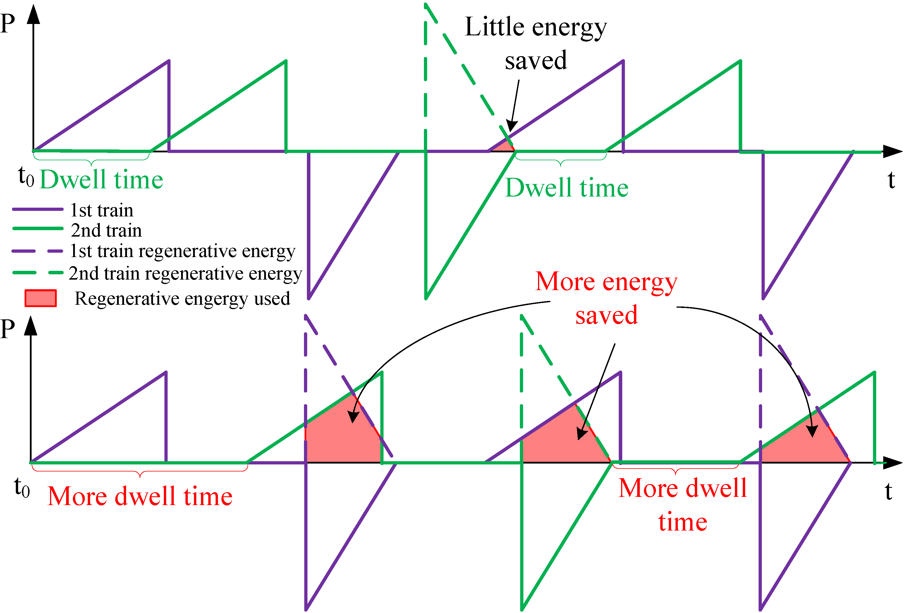
2.1. Timetable Optimization


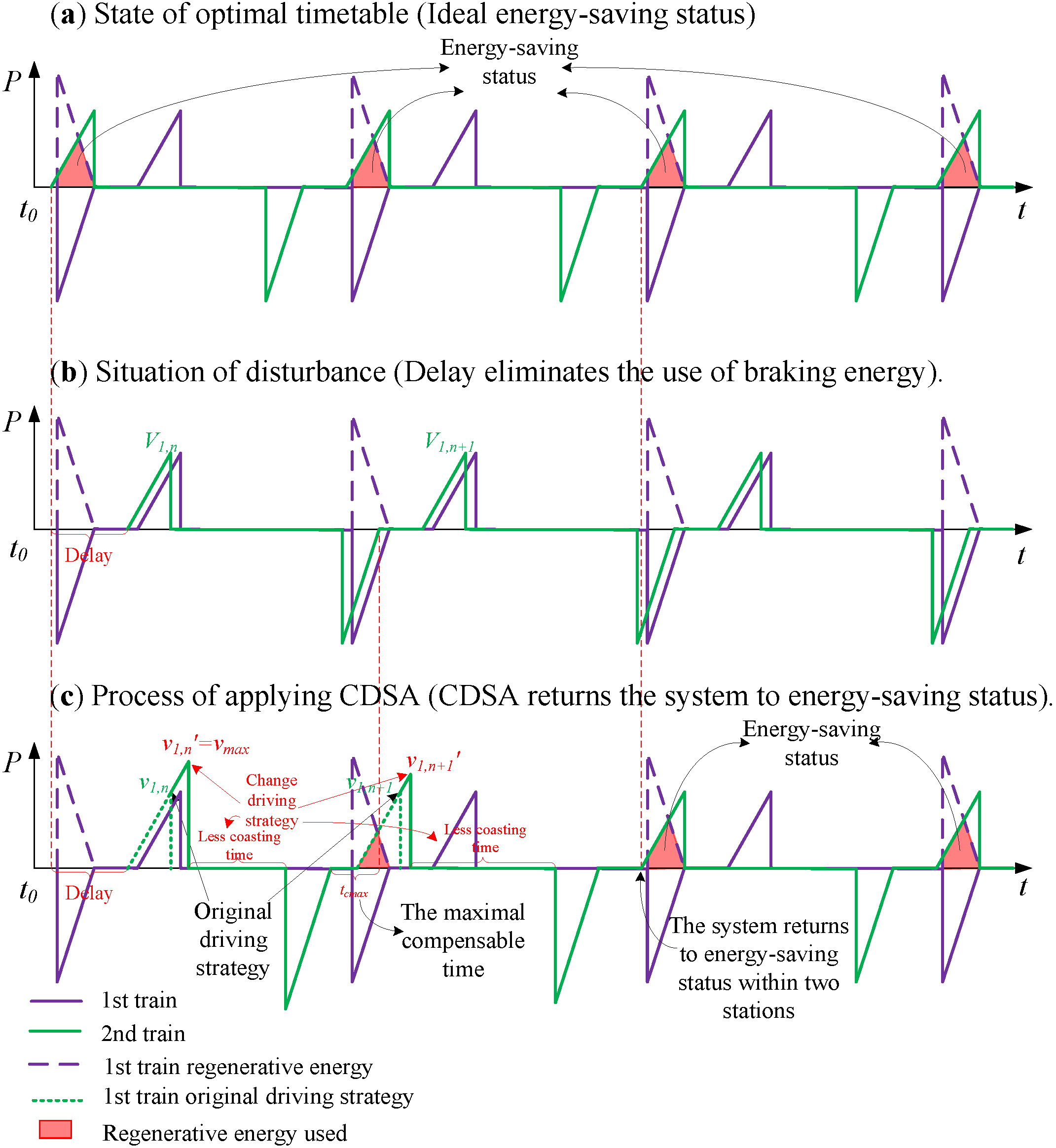
2.2. Compensational Driving Strategy Algorithm
- 1
- Driving with maximal acceleration;
- 2
- Traveling with constant speed (cruising);
- 3
- Coasting;
- 4
- Braking to target with maximal deceleration;
- 5
- Waiting for passengers to board the train (dwelling).


3. Case Study: Shanghai Metro Line One
3.1. Experiment Data and Parameters

- 1
- The experiment was done on a separate power supply system designed especially for the test and maintenance, so the supply capacity is limited.
- 2
- There were no other trains in the same supply network.
- 3
- During the experiment, the test metro train was unloaded. That means the mass of the whole test metro train is just its own mass, which is 296 tons.
- 4
- Most of the auxiliary electric devices, like air-conditioners, were switched off during the experiment.
- 5
- The metro train is composed of six cars. All the measurements were taken from one of the cars.


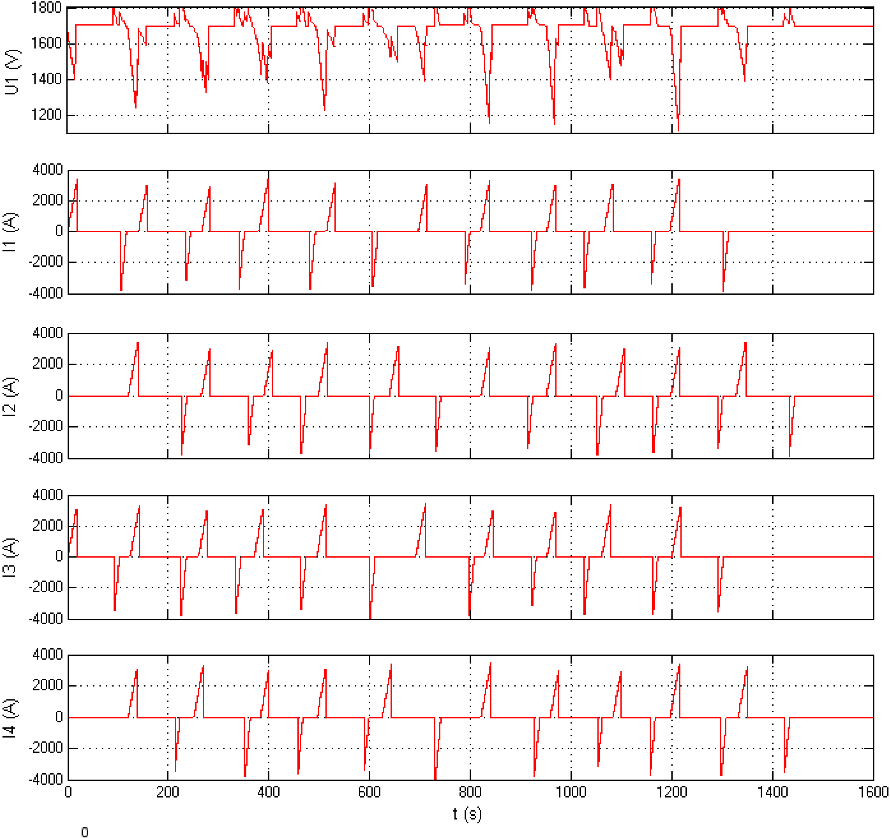
3.2. Modeling of the Pilot Metro System

| Segment No. | Starting station | Stopping station | Distance (m) | v1,n (km/h) |
|---|---|---|---|---|
| 1 | Xujiahui | Hengshan Road | 1473 | 57.7 |
| 2 | Hengshan Road | Changshu Road | 1156 | 51.1 |
| 3 | Changshu Road | South Shanxi Road | 939 | 51.3 |
| 4 | South Shanxi Road | South Huangpi Road | 1407 | 57.4 |
| 5 | South Huangpi Road | People’s Square | 1198 | 53.4 |


3.3. Applying EOM to the System
3.3.1. Specifying the Driving Strategy
| Parameter | a1 (m/s2) | a2 (m/s2) | a3 (m/s2) |
|---|---|---|---|
| Value | 0.8333 | −0.0363 | −1.1723 |

| Segment No. | t1,n (s) | t2,n (s) | t3,n (s) | v1,n (m/s) | v2,n (m/s2) |
|---|---|---|---|---|---|
| 1 | 19.23 | 86.31 | 11.00 | 16.03 | 12.89 |
| 2 | 17.03 | 76.50 | 9.74 | 14.19 | 11.42 |
| 3 | 17.10 | 57.06 | 10.39 | 14.25 | 12.18 |
| 4 | 19.13 | 81.80 | 11.07 | 15.94 | 12.98 |
| 5 | 17.80 | 74.42 | 10.35 | 14.83 | 12.13 |
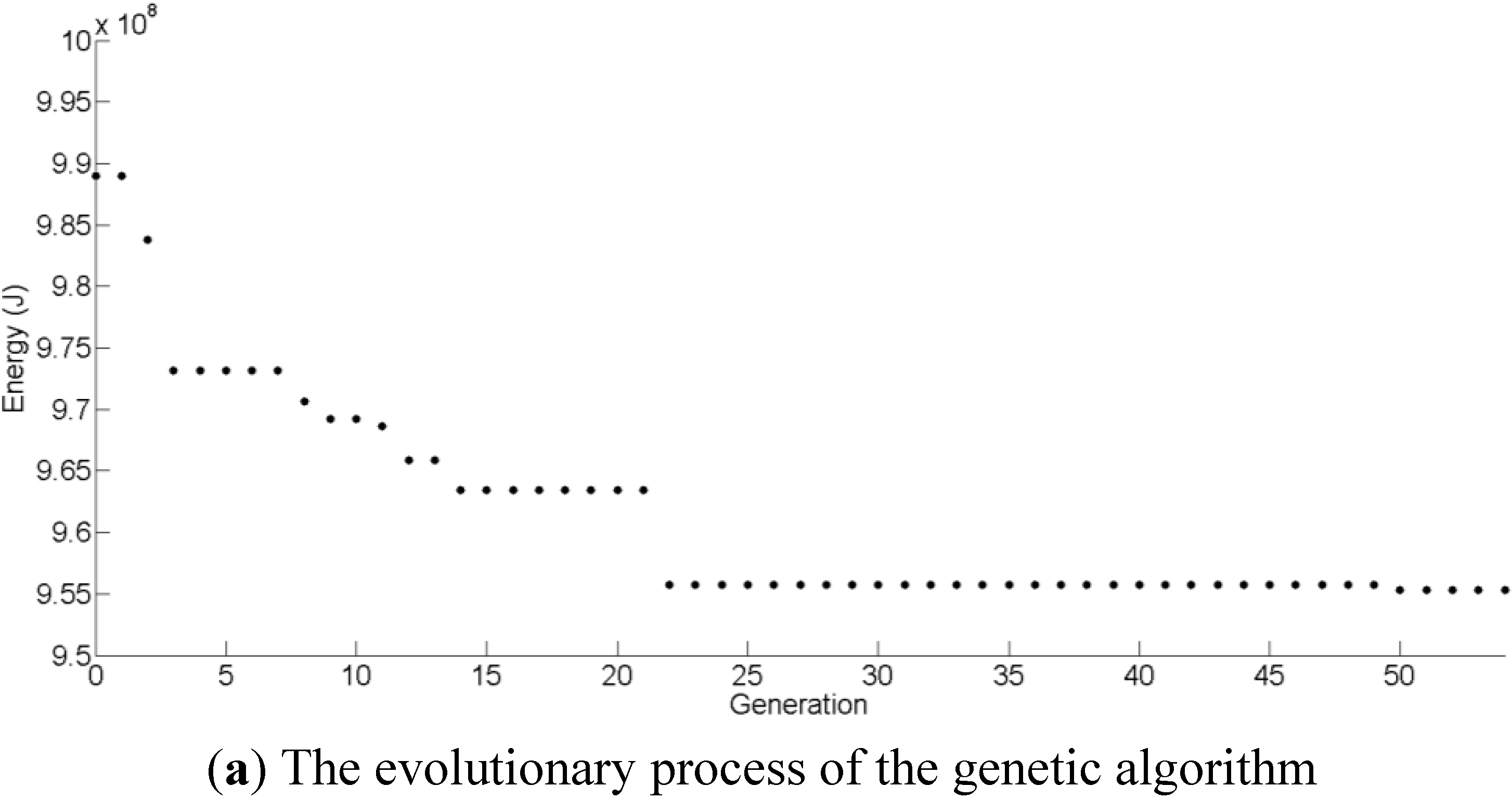
3.3.2. Using TO


3.3.3. Applying CDSA
| Trains depart from this end | Xujiahui | Hengshan Road | Changshu Road | South Shanxi Road | South Huangpi Road | People’s Square | Trains depart from this end | |||||||
|---|---|---|---|---|---|---|---|---|---|---|---|---|---|---|
| Train 1 | Forward | 8:00:00 |  | 8:02:21 | | 8:04:26 | | 8:06:19 | | 8:08:33 |  | 8:11:36 | ||
| Backward | 8:23:12 |  | 8:19:55 | | 8:17:45 | | 8:15:52 | | 8:13:40 |  | ||||
| Train 2 | Forward | 8:02:00 | | 8:04:26 | | 8:06:30 | | 8:08:17 | | 8:10:38 | | 8:13:41 | ||
| Backward | 8:25:24 | | 8:22:07 | | 8:19:58 | | 8:18:09 | | 8:15:51 | | ||||
| 8:11:31 | | 8:08:14 | | 8:06:10 | | 8:04:20 | | 8:02:04 | | 8:00:00 | Backward | Train 3 | ||
| | 8:13:57 | | 8:16:02 | | 8:17:50 | | 8:20:09 | | 8:23:12 | Forward | ||||
| 8:13:41 | | 8:10:24 | | 8:08:15 | | 8:06:23 | | 8:04:11 | | 8:02:00 | Backward | Train 4 | ||
| | 8:15:58 | | 8:18:03 | | 8:19:56 | | 8:22:11 | | 8:25:14 | Forward | ||||

3.4. The Energy-Saving Analysis of EOM
| Different situations | Average energy consumption (MJ) | Average energy saving (MJ) | Average energy-saving percentage (%) |
|---|---|---|---|
| Original timetable | 1007.05 | 0 | 0 |
| Optimal timetable | 955.46 | 51.59 | 5.12 |
| Disturbance without CDSA | 984.71 | 22.34 | 2.22 |
| Disturbance with CDSA | 966.39 | 40.66 | 4.04 |

4. Conclusions
Nomenclature
| E | total energy-consumption of the system |
| Q | number of substations of power supply for the metro system |
| Uj | DC voltage of the jth substation |
| Ij | DC current of the jth substation |
| Fr | running resistance |
| Ln | distance between the nth and (n + 1)th station |
| v1,n | instant speed at the end of accelerating between the nth and (n + 1)th station |
| v2,n | instant speed at the end of coasting between the nth and (n + 1)th station |
| vmax | maximal speed of the train |
| vlimit | speed limitation |
| a1,n | acceleration of accelerating between the nth and (n + 1)th station |
| a2,n | acceleration of coasting between the nth and (n + 1)th station |
| a3,n | acceleration of braking between the nth and (n + 1)th station |
| tstart,n | starting time of leaving the nth station |
| t1,n | duration of accelerating between the nth and (n + 1)th station |
| t2,n | duration of coasting between the nth and (n + 1)th station |
| t3,n | duration of braking between the nth and (n + 1)th station |
| tn | total running time between the nth and (n + 1)th station |
| t4,n | duration of dwelling between the nth and (n + 1)th station |
| td,n | time delay caused by disturbance between the nth and(n + 1)th station |
| tcmax,n | maximal compensable time delay between the nth and (n + 1)th station |
| tf | total travelling time of the system |
Acknowledgments
Author Contributions
Conflicts of Interest
References
- Shanghai metro. Available online: http://en.wikipedia.org/wiki/Shanghai_metro (accessed on 25 June 2014).
- González-Gil, A.; Palacin, R.; Batty, P.; Powell, J. A systems approach to reduce urban rail energy consumption. Energy Conver. Manag. 2014, 80, 509–524. [Google Scholar] [CrossRef]
- Howlett, P.; Milroy, I.; Pudney, P. Energy-efficient train control. Control Eng. Pract. 1994, 2, 193–200. [Google Scholar] [CrossRef]
- Chevrier, R. An evolutionary multi-objective approach for speed tuning optimization with energy saving in railway management. In Proceedings of the 13th IEEE International Conference on Intelligent Transportation Systems, Funchal, Portugal, 19–22 September 2010; pp. 279–284.
- Chevrier, R.; Pellegrini, P.; Rodriguez, J. Energy saving in railway timetabling: A bi-objective evolutionary approach for computing alternative running times. Transp. Res. C Emerg. Technol. 2013, 37, 20–41. [Google Scholar] [CrossRef]
- Howlett, P. The optimal control of a train. Ann. Oper. Res. 2000, 98, 65–87. [Google Scholar] [CrossRef]
- Howlett, P. Optimal strategies for the control of a train. Automatica 1996, 32, 519–532. [Google Scholar] [CrossRef]
- Jiaxin, C.; Howlett, P. A note on the calculation of optimal strategies for the minimization of fuel consumption in the control of trains. IEEE Trans. Autom. Control 1993, 38, 1730–1734. [Google Scholar] [CrossRef]
- Liu, R.R.; Golovitcher, I.M. Energy-efficient operation of rail vehicles. Trans. Res. A Policy Pract. 2003, 37, 917–932. [Google Scholar] [CrossRef]
- Khmelnitsky, E. On an optimal control problem of train operation. IEEE Trans. Autom. Control 2000, 45, 1257–1266. [Google Scholar] [CrossRef]
- Bocharnikov, Y.; Tobias, A.; Roberts, C.; Hillmansen, S.; Goodman, C. Optimal driving strategy for traction energy saving on dc suburban railways. IET Electr. Power Appl. 2007, 1, 675–682. [Google Scholar] [CrossRef]
- Domínguez, M.; Fernández-Cardador, A.; Cucala, A.P.; Gonsalves, T.; Fernández, A. Multi objective particle swarm optimization algorithm for the design of efficient ato speed profiles in metro lines. Eng. Appl. Artif. Intel. 2014, 29, 43–53. [Google Scholar] [CrossRef]
- Domínguez, M.; Fernández-Cardador, A.; Cucala, A.P.; Pecharromán, R.R. Energy savings in metropolitan railway substations through regenerative energy recovery and optimal design of ato speed profiles. IEEE Trans. Autom. Sci. Eng. 2012, 9, 496–504. [Google Scholar] [CrossRef]
- Domínguez, M.; Fernández, A.; Cucala, A.; Lukaszewicz, P. Optimal design of metro automatic train operation speed profiles for reducing energy consumption. Proc. Inst. Mech. Eng. F J. Rail Rapid Transit 2011, 225, 463–474. [Google Scholar] [CrossRef]
- Lu, S.; Weston, P.; Hillmansen, S.; Gooi, H.B.; Roberts, C. Increasing the regenerative braking energy for railway vehicles. IEEE Trans. Intel. Transp. Syst. 2014, 99, 1–10. [Google Scholar]
- Liu, C.; Li, F.; Ma, L.P.; Cheng, H.M. Advanced materials for energy storage. Adv. Mater. 2010, 22, E28–E62. [Google Scholar] [CrossRef] [PubMed]
- Wang, G.; Zhang, L.; Zhang, J. A review of electrode materials for electrochemical supercapacitors. Chem. Soc. Rev. 2012, 41, 797–828. [Google Scholar] [CrossRef] [PubMed]
- Burke, A.; Miller, M. The power capability of ultracapacitors and lithium batteries for electric and hybrid vehicle applications. J. Power Sources 2011, 196, 514–522. [Google Scholar] [CrossRef]
- Hammar, A.; Venet, P.; Lallemand, R.; Coquery, G.; Rojat, G. Study of accelerated aging of supercapacitors for transport applications. IEEE Trans. Ind. Electron. 2010, 57, 3972–3979. [Google Scholar] [CrossRef]
- Sharma, P.; Bhatti, T.S. A review on electrochemical double-layer capacitors. Energy Convers. Manag. 2010, 51, 2901–2912. [Google Scholar] [CrossRef]
- Iannuzzi, D.; Tricoli, P. Metro trains equipped onboard with supercapacitors: A control technique for energy saving. In Proceedings of the IEEE International Symposium on Power Electronics Electrical Drives Automation and Motion (SPEEDAM), Pisa, Italy, 14–16 June 2010; pp. 750–756.
- Liu, H.; Jiang, J. Flywheel energy storage—An upswing technology for energy sustainability. Energy Build. 2007, 39, 599–604. [Google Scholar] [CrossRef]
- Jefferson, C.; Ackerman, M. A flywheel variator energy storage system. Energy Convers. Manag. 1996, 37, 1481–1491. [Google Scholar] [CrossRef]
- Suzuki, Y.; Koyanagi, A.; Kobayashi, M.; Shimada, R. Novel applications of the flywheel energy storage system. Energy 2005, 30, 2128–2143. [Google Scholar] [CrossRef]
- Tzeng, J.; Emerson, R.; Moy, P. Composite flywheels for energy storage. Compos. Sci. Technol. 2006, 66, 2520–2527. [Google Scholar] [CrossRef]
- Bolund, B.; Bernhoff, H.; Leijon, M. Flywheel energy and power storage systems. Renew. Sustain. Energy Rev. 2007, 11, 235–258. [Google Scholar] [CrossRef]
- Kraytsberg, A.; Ein-Eli, Y. Review on Li–air batteries—Opportunities, limitations and perspective. J. Power Sources 2011, 196, 886–893. [Google Scholar] [CrossRef]
- Ellis, B.L.; Nazar, L.F. Sodium and sodium-ion energy storage batteries. Curr. Opinion Solid State Mater. Sci. 2012, 16, 168–177. [Google Scholar] [CrossRef]
- Mukherjee, R.; Krishnan, R.; Lu, T.-M.; Koratkar, N. Nanostructured electrodes for high-power lithium ion batteries. Nano Energy 2012, 1, 518–533. [Google Scholar] [CrossRef]
- Kritzer, P. Separators for nickel metal hydride and nickel cadmium batteries designed to reduce self-discharge rates. J. Power Sources 2004, 137, 317–321. [Google Scholar] [CrossRef]
- Czerwiński, A.; Obrębowski, S.; Rogulski, Z. New high-energy lead-acid battery with reticulated vitreous carbon as a carrier and current collector. J. Power Sources 2012, 198, 378–382. [Google Scholar]
- González-Gil, A.; Palacin, R.; Batty, P. Sustainable urban rail systems: Strategies and technologies for optimal management of regenerative braking energy. Energy Convers. Manag. 2013, 75, 374–388. [Google Scholar] [CrossRef]
- Chen, J.F.; Lin, R.L.; Liu, Y.C. Optimization of an mrt train schedule: Reducing maximum traction power by using genetic algorithms. IEEE Trans. Power Syst. 2005, 20, 1366–1372. [Google Scholar] [CrossRef]
- Nasri, A.; Moghadam, M.F.; Mokhtari, H. Timetable optimization for maximum usage of regenerative energy of braking in electrical railway systems. In Proceedings of IEEE International Symposium on Power Electronics Electrical Drives Automation and Motion (SPEEDAM), Pisa, Italy, 14–16 June 2010; pp. 1218–1221.
- Albrecht, T. Reducing power peaks and energy consumption in rail transit systems by simultaneous train running time control. In Computers in Railways IX; WIT Press: Southampton, UK, 2004; pp. 885–894. [Google Scholar]
- Fournier, D.; Mulard, D.; Fages, F. Energy optimization of metro timetables: A hybrid approach. In Proceedings of the 18th International Conference on Principles and Practice of Constraint Programming (CP 12), Québec, QC, Canada, 8–12 October 2012; pp. 7–12.
- Bocharnikov, Y.; Tobias, A.; Roberts, C. Reduction of train and net energy consumption using genetic algorithms for trajectory optimisation. In Proceedings of IET Conference on Railway Traction Systems (RTS 2010), Birmingham, UK, 13–15 April 2010; pp. 1–5.
- Kim, K.M.; Oh, S.M.; Han, M. A mathematical approach for reducing the maximum traction energy: The case of Korean MRT trains. In Proceedings of the International MultiConference of Engineers and Computer Scientists, Hong Kong, China, 17–19 March 2010; pp. 2169–2173.
- Peña-Alcaraz, M.; Fernández, A.; Cucala, A.P.; Ramos, A.; Pecharromán, R.R. Optimal underground timetable design based on power flow for maximizing the use of regenerative-braking energy. Proc. Inst. Mech. Eng. F J. Rail Rapid Transit 2012, 226, 397–408. [Google Scholar] [CrossRef]
- Yang, X.; Ning, B.; Li, X.; Tang, T. A two-objective timetable optimization model in subway systems. IEEE Trans. Intel. Transp. Syst. 2014, 15, 1–9. [Google Scholar] [CrossRef]
- Li, X.; Lo, H.K. An energy-efficient scheduling and speed control approach for metro rail operations. Transp. Res. B Methodol. 2014, 64, 73–89. [Google Scholar] [CrossRef]
- Su, S.; Li, X.; Tang, T. A subway train timetable optimization approach based on energy-efficient operation strategy. IEEE Trans. Intel. Transp. Syst. 2013, 14, 883–893. [Google Scholar] [CrossRef]
- Su, S.; Tang, T.; Li, X.; Gao, Z. Optimization of multitrain operations in a subway system. IEEE Trans. Intel. Transp. Syst. 2014, 15, 673–684. [Google Scholar] [CrossRef]
- Deep, K.; Singh, K.P.; Kansal, M.; Mohan, C. A real coded genetic algorithm for solving integer and mixed integer optimization problems. Appl. Math. Comput. 2009, 212, 505–518. [Google Scholar] [CrossRef]
- Strobel, H.; Horn, P. On energy-optimum control of train movement with phase constraints. Electr. Inform. Energy Techn. J. 1973, 6, 304–308. [Google Scholar]
- Albrecht, T.; Oettich, S. A new integrated approach to dynamic schedule synchronization and energy-saving train control. In Computers in Railways VIII; WIT Press: Southampton, UK, 2002; pp. 847–856. [Google Scholar]
- Goodman, C. Overview of electric railway systems and the calculation of train performance. In Proceedings of the IET Professional Development course on Electric Traction Systems, Manchester, UK, 3–7 November 2008; pp. 1–24.
- Goodman, C.; Sin, L. DC railway power network solutions by diakoptics. In Proceedings of the Railroad Conference 1994 ASME/IEEE Joint (in Conjunction with Area 1994 Annual Technical Conference) In IEEE Railroad Conference, Chicago, IL, USA, 22–24 March 1994; pp. 103–110.
- Hammersley, J.M.; Handscomb, D.C. Monte Carlo Methods; Springer: Berlin, Germany, 1964. [Google Scholar]
© 2014 by the authors; licensee MDPI, Basel, Switzerland. This article is an open access article distributed under the terms and conditions of the Creative Commons Attribution license (http://creativecommons.org/licenses/by/4.0/).
Share and Cite
Gong, C.; Zhang, S.; Zhang, F.; Jiang, J.; Wang, X. An Integrated Energy-Efficient Operation Methodology for Metro Systems Based on a Real Case of Shanghai Metro Line One. Energies 2014, 7, 7305-7329. https://0-doi-org.brum.beds.ac.uk/10.3390/en7117305
Gong C, Zhang S, Zhang F, Jiang J, Wang X. An Integrated Energy-Efficient Operation Methodology for Metro Systems Based on a Real Case of Shanghai Metro Line One. Energies. 2014; 7(11):7305-7329. https://0-doi-org.brum.beds.ac.uk/10.3390/en7117305
Chicago/Turabian StyleGong, Cheng, Shiwen Zhang, Feng Zhang, Jianguo Jiang, and Xinheng Wang. 2014. "An Integrated Energy-Efficient Operation Methodology for Metro Systems Based on a Real Case of Shanghai Metro Line One" Energies 7, no. 11: 7305-7329. https://0-doi-org.brum.beds.ac.uk/10.3390/en7117305