Article

Flow Regime Changes: From Impounding a Temperate Lowland River to Small Hydropower Operations

Institute of Water Resources Engineering, Aleksandras Stulginskis University, 10 Universiteto str., Akademija, Kaunas District LT-53361, Lithuania
*
Author to whom correspondence should be addressed.
Energies 2015, 8(7), 7478-7501; https://0-doi-org.brum.beds.ac.uk/10.3390/en8077478
Submission received: 19 May 2015 / Revised: 14 July 2015 / Accepted: 16 July 2015 / Published: 22 July 2015
(This article belongs to the Special Issue Energy Policy and Climate Change)

Abstract

:
This article discusses the environmental issues facing small hydropower plants (SHPs) operating in temperate lowland rivers of Lithuania. The research subjects are two medium head reservoir type hydro schemes considered within a context of the global fleet of SHPs in the country. This research considers general abiotic indicators (flow, level, water retention time in the reservoirs) of the stream that may affect the aquatic systems. The main idea was to test whether the hydrologic regime has been altered by small hydropower dams. The analysis of changes in abiotic indicators is a complex process, including both pre- and post-reservoir construction and post commissioning of the SHPs under operation. Downstream hydrograph (flow and stage) ramping is also an issue for operating SHPs that can result in temporary rapid changes in flow and consequently negatively impact aquatic resources. This ramping has been quantitatively evaluated. To avoid the risk of excessive flow ramping, the types of turbines available were evaluated and the most suitable types for the natural river flow regime were identified. The results of this study are to allow for new hydro schemes or upgrades to use water resources in a more sustainable way.

1. Introduction

Humans often modify rivers to meet specific objectives, including hydropower generation. Flexibility in the timing of water use is a primary reason for regulating rivers. It is accepted that the construction of dams causes hydrologic alterations with consequent changes in ecological conditions. However, the effect of the impact depends on many factors and has to be considered on a case by case basis. For example, irrigation dams have completely different hydrologic alterations than hydropower operations.
The vast majority of studies considering these issues are based on large hydropower plants (HP) or large dams, where impacts are obvious. However, small hydropower plants (SHP) cannot be treated as a scaled down version of the large dams. A literature review has shown that there is a lack of associated studies, especially for low to medium head facilities operating in temperate lowland rivers.
Hydropower plants are divided into different categories according to their installed power (P), which are usually small (p < 10 MW), medium (10–100 MW) and large (>100 MW) [1]. However these classification systems may be very different elsewhere. The European standard of SHP plants has been set to the installed capacity (p < 10 MW), although many countries adopted a lower SHP limit than indicated in ESHA website [2]. A number of publications indicates that SHP impacts on the environment are not yet clearly revealed; therefore, they receive public support in the EU countries [3,4,5]. Well designed, monitored and sustainably operating SHPs may have a smaller impact on the ecosystem, if this is the case, they may be regarded as “environmentally friendly” [6,7]. The intensive land use for agriculture plays a more important role in terms of environmental impacts on the water quality of small lowland rivers than deployed SHP dams [8].
In contrast to the outline above, there are studies suggesting much more significant effects of SHPs [9,10]. The results of Kibler and Tullos [11] revealed that the biophysical impact of small hydropower plants in China might exceed even those of large hydropower plants, particularly with regard to habitat security and hydrologic change. However, it should be noted that in China, the small hydro capacity threshold is considered to be below 50 MW [1].
The EU Water Framework Directive (WFD) notes that hydropower has hydromorphological effects on the aquatic environment [12]. Many of these effects can be minimized; however, some effects are irreversible and it is impossible to achieve a good ecological status of the water body in accordance with WFD requirements [13].
Numerous metrics have been developed to represent the magnitude and direction of hydrologic alteration. The typical approach is the Flow Duration Curve (FDC) method, widely used in pre-post impact assessment of multipurpose uses of dams, e.g., hydropower [14,15,16]. Richter et al. [17], Olden and Poff [18] assessed and offered from three dozen to more than a hundred and fifty Indicators of Hydrologic alteration (IHA), which could be used for pre-post evaluations in different flow regime situations [19]. The prevailing opinion is that in most rivers, more than 90% of the flow variation can be explained by several statistically significant criteria [14]. Some hydrological indices are based on the average daily flow rate, which does not reflect irregularities of hydro plant operations within 24 h (e.g., hydropeaking or ramping). Moreover, not all indices can be applied equally to large and small hydropower plants. Any impoundment in spatial and temporal terms affects river flow regimes and global river environments. To represent quantitatively the spatial and temporal intensity of the water mass (inflow or outflow) in the control area, some indicators were proposed [20,21] which can be described using a number of terms e.g., Water Residence, Retention, Exposure, Turnover or Exchange time.
The ratio of storage capacity to mean annual flow has been used previously, for example by Brune [22], as the independent variable from which to predict reservoir trap efficiency. Impounded runoff index (IR) was used for large-scale dam affects to flow regime in California and Spain [23]. It should be noted that it is the dimensionless indicator. For example, an IR of 1 implies an average residence time of 1 year. Similarly to IR, a more detailed index D designated for reservoir hydropower plants with regard to the retention of cumulative inflow for a certain period of time at upstream storage was proposed [24]. According to the water retention time in reservoir or its filling period expressed in hours, HP plants can be divided into 3 groups: (a) run-of-river; (b) pondage; and (c) storage (Table 1). Water retention time (reservoir filling period D in hours) can be determined as follows:
D = V u Q 0 , [ m 3 m 3 / h ]
where Vu—useful capacity of reservoir, designated for power generation, m3 and Q0—inflow into reservoir (annual mean flow), m3/h.
The smaller the reservoir capacity and the higher the inflow into it, the less regulated natural flow will be assured. It can be accepted that RoR developments with D ≤ 2 h have a relatively minimal impact on the river flow regime.
The alternative indicator closely related to water retention time is K (Table 2). It is a percentage of the useful reservoir capacity to the volume of annual inflow [16,25]. To distinguish between flowing waters (rivers) and stagnant waters (lakes or reservoirs) K limit was proposed K = 100 [26].
Table 1. Classification of hydropower plants according to the retention time of the cumulative inflow into reservoir.
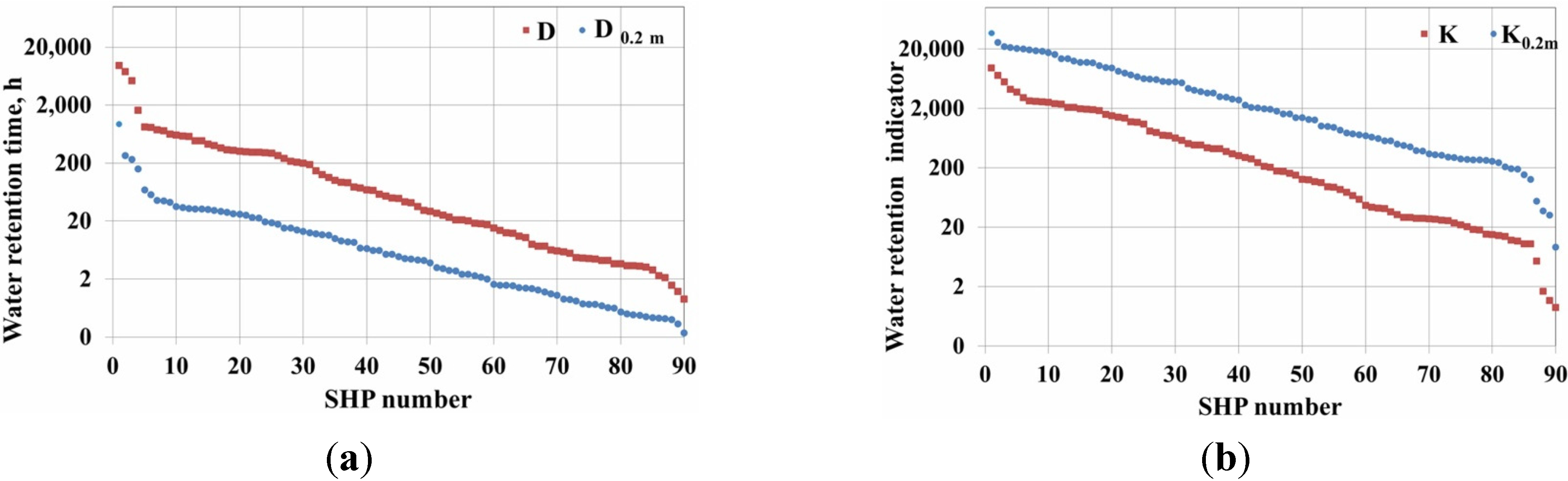
The Mode of Operation or Development TypeWater Retention Time in Reservoir (D)Comments
Run-of-river (RoR)D ≤ 2 h (~0.1 day)No possibilities to significantly regulate flow
Pondage2 h < D < 400 h (~17 days)Daily or weekly river flow regulation. Stores water at off-peak times and releases water through turbines at peak times
StorageD ≥ 400 hLong-term impounding of water to meet seasonal and annual fluctuations in water availability. Not typical for an SHP
Note: Compilation is based on [24].
Table 2. Water retention indicator.
Water Retention Indicator K 11010020050010002000
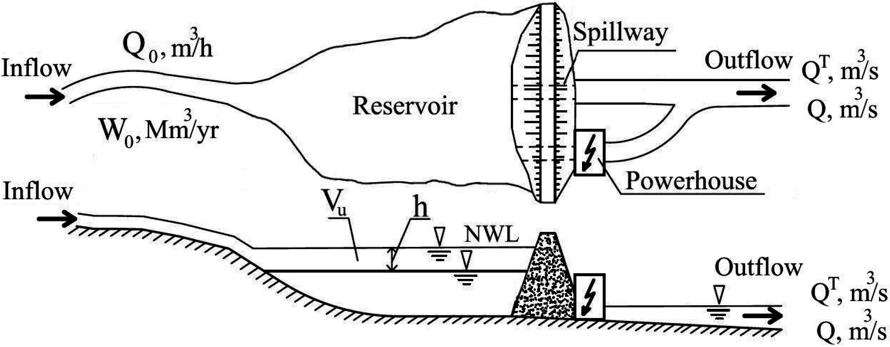
Reservoir Useful Capacity, Vu (Percentage of Volume of Annual Inflow)1001010.50.20.10.05
Water Retention Time (Days)36536.53.651.820.730.360.18
Water Body State“Stagnant” (lake)       “Running” (stream or river)
Although D and K are meaningfully related, their key estimates in the above tables have not been explicitly based. They only reflect the annual inflow transformation regardless of seasonal or shorter duration flow variations. In addition, RoR developments (small to medium hydro) can be described as follows [27,28,29]:
  • Turbines use the natural flow of the river with very little alteration to the terrain stream channel at the site and little impoundment of the water.
  • A type of hydro project that releases water at the same rate as the natural flow of the river (outflow equals inflow).
Run-of-river power projects are sometimes known as “small hydro” projects, though not all are small. References can be found in publications of hydropower plants with reservoir areas of several hundred square kilometres and more that are attributed to RoR projects [30]. For instance, in Austria, most of conventional large hydropower plants are considered RoR plants [31].
A simple sketch of a hydropower plant associated with a small reservoir provides additional explanations on the above mentioned indicators (Figure 1). The operation of some hydropower plants may lead to rapid and frequent changes in flow regimes, usually as a result of turbine start-up or shut-down, or in response to changes in electrical load. This mode of the operation, called hydropeaking or flow ramping, may have adverse impacts on the ecological integrity of streams and rivers. The negative effects of hydropeaking to the downstream river were first documented in Europe at the end of 1930. According to Bain [32], the first environmental impact studies in North America, related to this mode of operation, appeared in 1970s. Currently, there are plenty of investigations demonstrating the biological effects of this phenomenon, including its mitigation measures [33,34,35,36]. There is an obvious tendency to note that hydropeaking is mostly attributed to the hydro operations of storage power plants [37]. In run-of-river plants, hydropeaking is only observed following the emergency shut-down of turbines—a very rare occurrence, for instance, in Switzerland [38].
Figure 1. River flow distribution in a hydropower scheme associated with an embankment dam. Notes: Annual inflow into reservoir: Q0, W0 (flow and volume, respectively), h—drawdown depth of reservoir corresponding to the useful capacity of reservoir (Vu) and designated for power generation. Outflow: QT—turbine flow, Q—river flow (spill, leakage, instream flow). NWL—normal water level.
Energies 08 07478 g001
A decade ago, Baumann and Klaus [39] reviewed more than 200 articles indicating a clear lack of knowledge about the ecological effect of hydropeaking, the same was confirmed [40]. Despite the abundance of publications on the interrelations of hydropeaking and riparian or shallow zone ecology the ability to describe, correlate and quantitatively estimate biological responses on hydropeaking today is still weak [14]. Bain [32] reviewed 43 cases of hydropeaking in US and Europe. The effects ranged in accordance to their significance from moderate to severe alterations of downstream river environments. By analysing the hydropeaking mode practiced on three medium-sized HP (P = 25–50 MW), it was found that it was not a significant threat to the river environment and its biota. The restriction of flow ramping rates of hydroelectric turbines located on a river with a medium-sized HP in Canada did not show significant differences in the majority of measured biotic parameters relative to a natural system. However, once ramping restrictions were lifted, some changes in biotic parameters were found [15,41].
The requirement to restore the natural flow regime of hydropower projects shifting from the peak to run-of-river mode is becoming more and more popular in the US [42,43] and Europe, including Lithuania [44]. It is widely believed that the run-of-river operation has to be mandatory to protect aqua biota. However, it reduces the production of electricity per flow unit and at the same decreases incomes [45]. Technical measures have been studied to reduce the effects of hydropeaking [14,37,46,47,48]. They can be structured into two main groups: Operational (non-structural) and structural (involving any physical construction). Structural measures or the application of river engineering techniques cannot be easily realisable. In Canada and the US, the ramping rate standards (non-structural measures) provide guidance to run-of-river developers and operators for proposed or operating hydropower projects [49].
In Lithuania, more than 1000 small and medium sized reservoirs are currently registered, of which more than 90 are SHPs and only one large conventional power plant, operating at Kaunas on the country’s largest river the Nemunas. It should be noted that the RoR operating mode for SHPs is an obligatory requirement in Lithuania.
An examination of the effects that small reservoirs have on the hydrological regime of Lithuanian rivers was carried out [16,50]. It was determined that the large, 100 MW Kaunas HP plant hydropeaking operations resulted in long-term river bed erosion on the Nemunas River [51]. In addition the SHP impacts on the downstream river flow were noted [52]. The findings from these studies indicate that no comprehensive research on the quantification of environmental issues due to rapid HP flow fluctuations on biotic systems in Lithuanian rivers was carried out. One exception was for macro invertebrate composition [53].
The main objective of this research was to investigate and quantify changes in the hydrological regime—abiotic indicators of a small lowland river with pre- and post-impoundments including further construction of small hydropower plants. To achieve this objective, the following tasks were carried out:
(1)
Past research focusing on SHPs operating in run-of-river mode on temperate lowland rivers was reviewed;
(2)
Historical flow and stage data to quantify the changes in flow regime pre- and post-river impoundment and after SHP construction was collected;
(3)
Hydrograph ramping key characteristics using the hourly data of flow/stage downstream power plants to determine the causes was assessed;
(4)
Measures to reduce the effects of SHPs by adapting turbines to the river natural flow were proposed.
Hydrologic regime here is understood in a simplified manner, notably, flow and stage fluctuations downstream from the river and storage timing upstream. The following are not in the scope of this paper: Impacts on water quality, riparian vegetation, fluvial geomorphology, and macro invertebrate and fish communities that must be underpinned by a sound hydraulic-hydrological analysis.

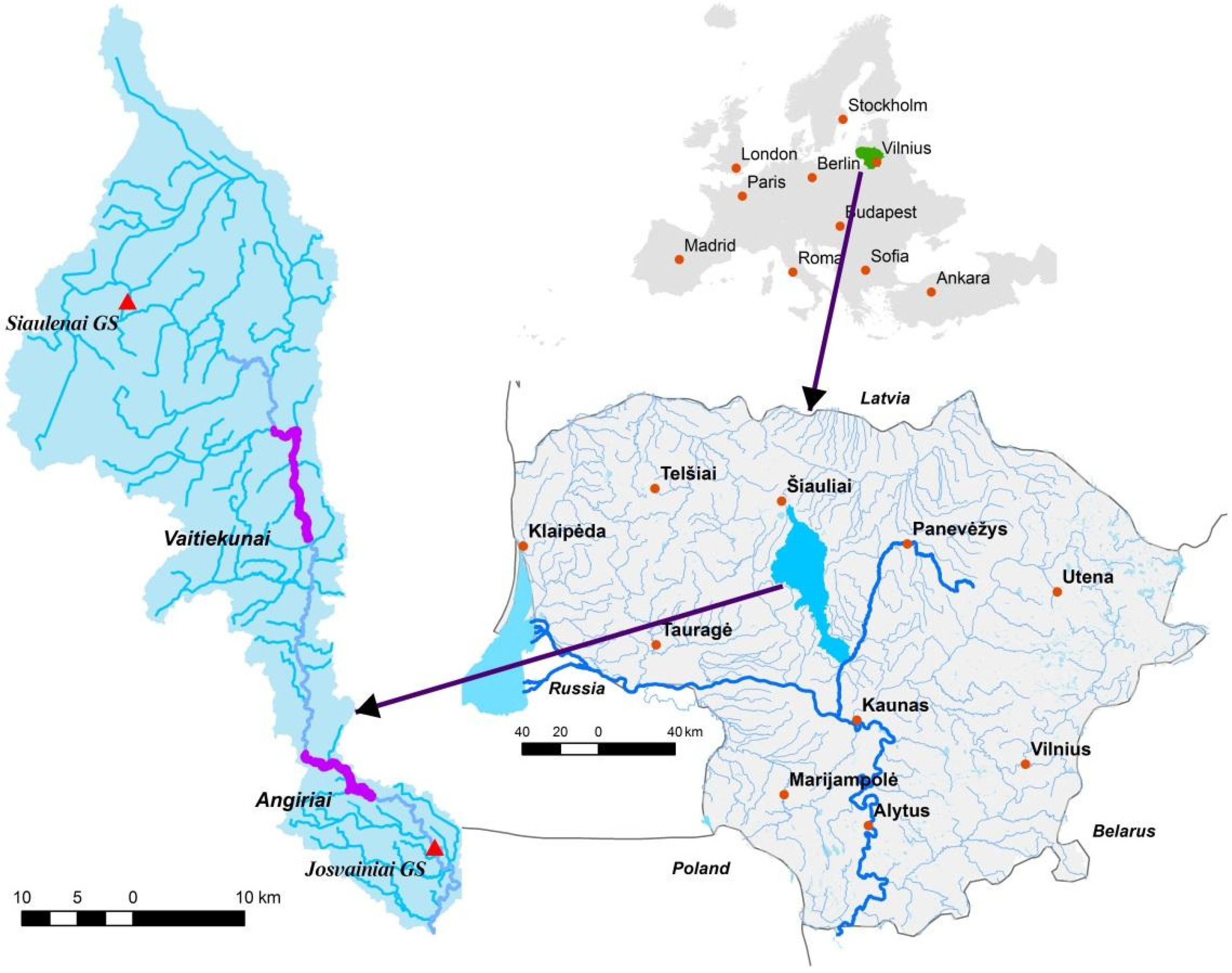
2. Materials and Methods

The study area is the Susve River Basin located in central Lithuania. There are two reservoirs, Angiriai and Vaitiekunai, which have SHPs installed downstream on the river (Figure 2). The Susve River is the largest tributary of the Nevezis River, which flows into the largest Lithuanian river—the Nemunas. Its length is 130 km, its catchment area is 1165 km2 and the average annual flow is 6.2 m3/s [54]. The average slope of the longitudinal river profile is 0.086%, with a gentle gradient upstream and a steeper gradient downstream. According to a number of authors [55], the catchment area over the past five decades has experienced significant land use changes, from deploying the tile drainage that reached 50% of the total catchment area in 1990, to increased woodland area (from 21% in 1960 to 31% in 2010). These changes influenced the hydrological regime, although estimates of the regime changes differ. The Susve River is not abundant in fish resources. The Lithuanian fish index LFI (0 = bad and 1 = very good) for the Susve River is between 0.19 below the Siaulenai gauging station (GS) and 0.42, on average, at its mouth. Sediment transport is not an issue in lowland rivers of the country. In this regard, the life span of reservoirs is long, and their useful capacity can be insignificantly changed during a long time period [16].
Figure 2. The catchment area of the Susve River with the location of the Angiriai and Vaitiekunai SHP reservoirs (purple color) and the Siaulenai and Josvainiai longstanding gauging stations (GS, red triangles).
Energies 08 07478 g002
Both reservoirs were built 35 years ago as water storage for irrigation at that time. After a couple decades, they were adjusted for hydropower (Table 3).
Table 3. Description of reservoirs and SHPs on the Susve River.
SHP NameDistance of the Mouth, kmCatchment Area A km2Mean annual Flow Q0 m3/sYear of Construction Reservoir/SHPReservoirSHPReservoir Filling Period “D
Surface Area km2Total Volume Mm3Installed Power MWTurbine Type and NumberSHP Discharge QT m3/sHead, mQT/Qe
Angiriai2510506.01980/19982.4815.61.3Propeller 210.2 (5.1 + 5.1)14.51523
Vaitiekunai607995.11979/20011.425.00.37Cross-flow 25.5 (5.2 + 0.3)9.71.415
The hydropower schemes involve an earth-fill dam with an integral and separated intake, and a powerhouse located at the dam toe (Figure 1). They are not traditional diversion schemes.
The Angiriai SHP in terms of the installed capacity is the third largest of the SHPs in the country, while Vaitiekunai SHP falls within the average. In line with the definition of International Commission on Large Dams [56], the dams are considered to be large (reservoir storage >3 Mm3, and dam height >5 m) and SHPs are medium head. Angiriai SHP turbines are propeller-type and consequently flow rate adjustment limits are very narrow. Cross-flow turbines are operating in the Vaitiekunai SHP; they are of varying capacity and flow regulation is very flexible. As a result, the ratio between the turbine minimum discharge Q m i n T and instream flow Qe is 10 times less than in the former plant. The standard flow measurements at Siaulenai and Josvainiai longstanding gauging stations were used (Table 4).
Table 4. Characteristic of the Susve River gauging stations.
Gauging StationDistance from the Mouth, kmA, km2Data Series LengthQ0Q0 V-XIQmaxQmax/Q0
Q0 XII-IIQ0maxQ0max/Q0
Josvainiai14.210801956–19996.2327247.4
2003–20146.232.75.2
Siaulenai108.61621940–19991.291.2964.750.2
2000–20141.316.144.75
The observation period of both GS is longer than 50 years; the samples are representative and unbiased and are free from significant diversion or regulation prior to dam construction. In addition, short-term series of recorded water levels at 1 hour time intervals upstream and downstream from the dams (including turbines discharge) of the SHPs were used. The Siaulenai GS can be considered as a reference station—upstream there is no flow regulation, in contrast to the Josvainiai GS. The latter is located downstream of both reservoirs and the flow data integrates both land use impacts and the effects of reservoirs with SHPs.
When evaluating the effect of any impact on the hydrological regime, it is important that the data, which is divided into separate periods, should be assessed in relation to the variations of the long-term data. It is necessary to ensure that the data chosen covers the necessary cycles and determine whether they have downward or upward trends, therefore, a review was made of the Susve at Josvainiai annual flow fluctuations in a light of a long-term historic flow data series of the Nemunas River at Smalininkai (sample exceeds more than 200 years). For this purpose, the most commonly used methods for the assessment are: Cumulative deviations, moving average or trend detection using statistical tests. The Mann-Kendal test was applied for trend detection for the annual average flow at Smalininkai and Josvainiai GS. Flow duration curves (FDC) were used for comparisons of flow regime in three selected periods, and in two subbasins monitored by the Siaulenai and Josvainiai gauging stations. FDC is considered to be not only one of the most popular methods of comparison [19,57], in addition its statistical parameters also enable the formulation of appropriate findings [58]. Periods of construction are excluded from analysed flow series. To obtain a more accurate analysis when comparing two subbasins with different catchment areas, in some cases flow data are presented as water depths in millimetres per day.
The terms hydropeaking and flow (stage) ramping are interchangeable in view of hydrological response. However, no SHP in Lithuania operates under the peaking mode; therefore, the expression “ramping” is more accurate. The notions flow and stage (hydrograph) ramping here are used concurrently.
General hydropeaking indicators were used in the study [14,43,48,59,60]. The results indicate that flow variability statistics should be quantified using subdaily datasets to accurately represent the nature of hydropower operations, especially for daily peaking facilities. For the purposes of this article, “ramping rate” refers to the rate of change in water flow (in cubic meters per second/per hour) or water level range (depth per unit time—cm/h). There can be either up-ramping or down-ramping rates. The first ramping indicator, HR1 (in the normalised form), represents river flow variations with respect to the river daily average flow due to start-up and shutdown turbines:
H R 1 = Q max T Q min T Q 0
where Q m a x T —turbine maximum discharge within 24 h; Q m i n T —turbine minimum discharge within 24 h and Q0—river daily mean discharge (inflow into reservoir).
If turbine flow is steady within a daily period, then the above difference in the numerator does not make sense: The ramping does not occur. The ideal case is when HR1d = 1 (inflow to a reservoir equals outflow).
The second indicator, ramping rate (HR2), describes the gradient in stage (or flow) change and is defined as the change in water level (flow) between two successive records divided by the observation time interval, as defined by:
H R 2 , i = W L i W L i 1 t i t i 1
where WLi—water level, cm at time ti, hour and WLi−1 water level at prior time ti−1.
There is no special flow or level ramping restrictions in force for SHPs in Lithuania. Restrictions are imposed only on SHP reservoir water level drawdowns (±10 cm of NWL), which, as observations show, have little effect on ramping characteristics downstream of power plants.
A field experiment was carried out to discover the mechanism of stage ramping at the Angiriai SHP downstream the river [16]. Before starting up two turbines at their full capacity (QT = 10.2 m3/s), inflow into the reservoir and outflow was minimal (only environmental flow—approx. 0.4 m3/s). It was the end of summer, which is the low flow season; the river channel was extensively vegetated. Water level data logger and gauge staffs (3 in total) were used to monitor water level fluctuations and traveling of a wave along the river reach at 4 locations (last one at some 8 km from SHP) induced by starting and shutting down turbines.

3. Results and Discussion

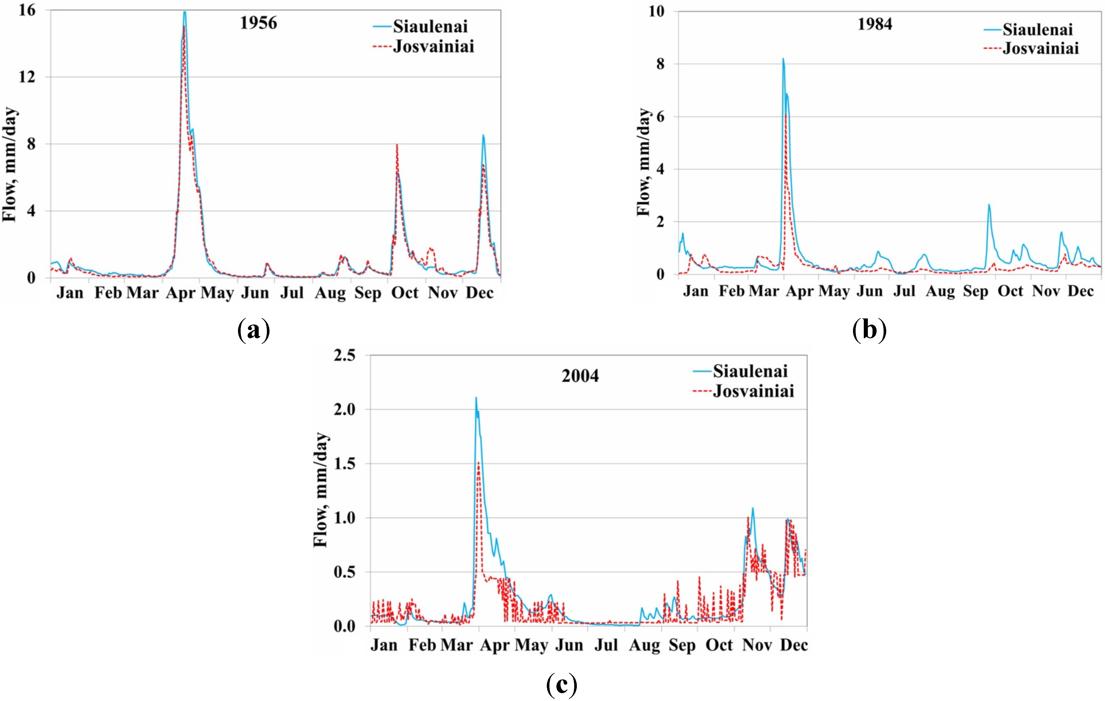
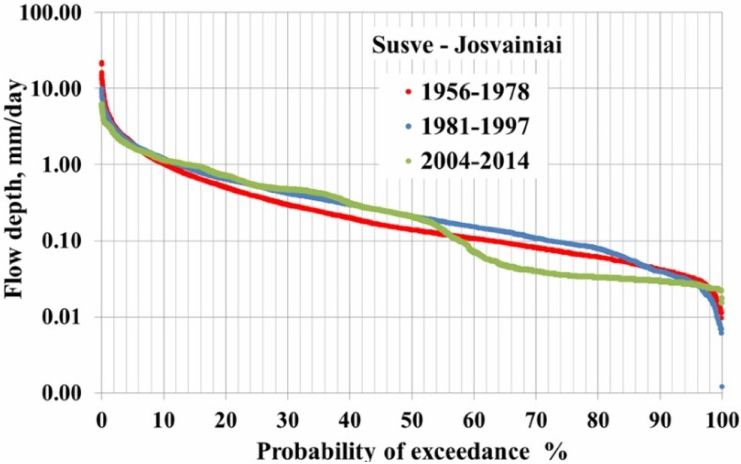
3.1. Pre- and Post-Impoundment Hydrologic Changes of the Susve River

Moving 11-year averages of long-term data show that the Susve River follows synchronical fluctuations of the Nemunas River and that the Susve flow covers two cycles of long-term fluctuations (Figure 3). According to the Mann-Kendal test, no statistically significant trends are detected for the annual average flow at Smalininkai and Josvainiai GS.
Figure 3. 11-year moving average flow (Qo) graphs for the Susve River at Josvainiai and the Nemunas River at Smalininkai.
Energies 08 07478 g003
Taking into account long-term fluctuations and knowing the dates of human interventions, the following three periods were selected:
  • Free flowing river (1956–1978);
  • Regulated river (2 impoundments in place) (1981–1997);
  • 2 SHPs deployed (2003–2014).
River flow regime can be clearly observed in daily flow hydrographs (Figure 4), representing each selected period.
Figure 4. Daily flow of selected years from different periods at Siaulenai (reference station, control river—no impact), and Josvainiai (impact of reservoirs and SHP) gauging stations. (a) 1956—pre-impoundment: No reservoirs at either subbasin; (b) 1984—post-impoundments: Vaitiekunai and Angiriai reservoirs without SHP; (c) 2004—SHPs are operating.
Energies 08 07478 g004
The year 1956 represents the first period showing synchronical flow at both stations and hydrographs almost overlapping with each other. In 1984, decreases of peak flow can be observed at Josvainiai GS due to what is known as the effect of flow transformation in the reservoir. In the third graph (2004), we already see the saw-type hydrograph of the Josvainiai GS, which is completely different from the Siaulenai GS, especially in low flow periods. Figure 4 illustrates evident impacts but does not give us the magnitudes of the impacts. The main parameters of descriptive statistics are presented in Table 5.
Table 5. Statistical parameters of analysed daily flow (mm/day) data.
PeriodGauging StationMeanMinMaxSTDCoefficient of VariationSkewnessKurtosis
1956–1978Siaulenai0.640.001124.751.302.047.24581.01
Josvainiai0.450.009621.761.052.337.52887.13
1981–1997Siaulenai0.680.003710.721.191.753.84618.16
Josvainiai0.480.00049.920.811.674.44227.74
2003–2010Siaulenai0.580.00856.080.841.462.7659.07
Josvainiai0.440.01526.180.651.472.99712.67
The high magnitudes of skewness indicate that no one analysed time series follows a normal distribution, although this parameter consistently decreases with each period. That points to the fact of influence of the construction of reservoirs, and the later installation of hydropower plants, on flow regime. Decreasing variation coefficients indicate that the flow regime becomes smoother in last two periods when the reservoirs are constructed and HP are installed. However, general statistics do not explain the impacts on seasonal daily flows.
Comparison of FDC in each period between two gauging stations—Siaulenai and Josvainiai—is presented in Figure 5 and a comparison FDCs of different periods at Josvainiai GS is presented in Figure 6. In the first period (1956–1978) (Figure 5a), the FDCs of two subbasins represent the situation without reservoirs in either subbasin. Curves do not overlap each other because of a different base flow that is slightly higher in the upper subbasin. The second period (1981–1997) (Figure 5b) gives almost overlapped curves in the lower part. Erected reservoirs slightly increase downstream flow in the dry season. This effect lifts up the lower part of Josvainiai FDC. The last period (2004–2014) (Figure 5c) gives the sharpest difference in the lower part of Josvainiai FDC. This can be explained by analysing the saw-shape hydrographs (Figure 4) of the last period. All of the peaks in the hydrographs are due to pulses when SHP turbines are started up or shut down. According to flow magnitudes, these pulses in FDC are moved to the left. At the same time, the rest of the flow magnitudes of the dry period are lower comparing to the Siaulenai GS flow what is the main reason of FDC drop down in interval from 60% to 90%.
Figure 5. Comparison of FDCs in each period between two gauging stations—Siaulenai and Josvainiai. (a) The first period (1956–1978); (b) The second period (1981–1997); (c) The last period (2004–2014).
Energies 08 07478 g005
Figure 6. Comparison of FDCs of different periods at Josvainiai GS.
Energies 08 07478 g006
To ensure that there are no impacts of any unknown factors that are upstream or downstream flow on the form of FDC, we compared curves of Josvainiai GS with each other (Figure 6). Here we see a similar situation. The FDC of the first two periods almost overlaps in the lower part and the third one differs greatly. To confirm the obtained visual facts, the FDCs of Josvainiai have been approximated applying Pearson type III distribution (Table 6). Both parameters—bias and RMSE—90 day and 180 day minima indicate the difference of the third period from the first two.
Table 6. Comparison of statistical parameters of approximated FDC by Pearson type III distribution.
PeriodFDC Parameters90 Day Minima180 Day Minima
Mean Q0 m3/sQ95 m3/sRMSEBias m3/sRMSEBias m3/s
1956–19780.4500.03190.0117−0.20590.0168−0.2294
1981–19970.4820.02800.0137−0.35180.0175−0.2377
2004–20140.4460.02640.0306−1.60320.0834−2.9760

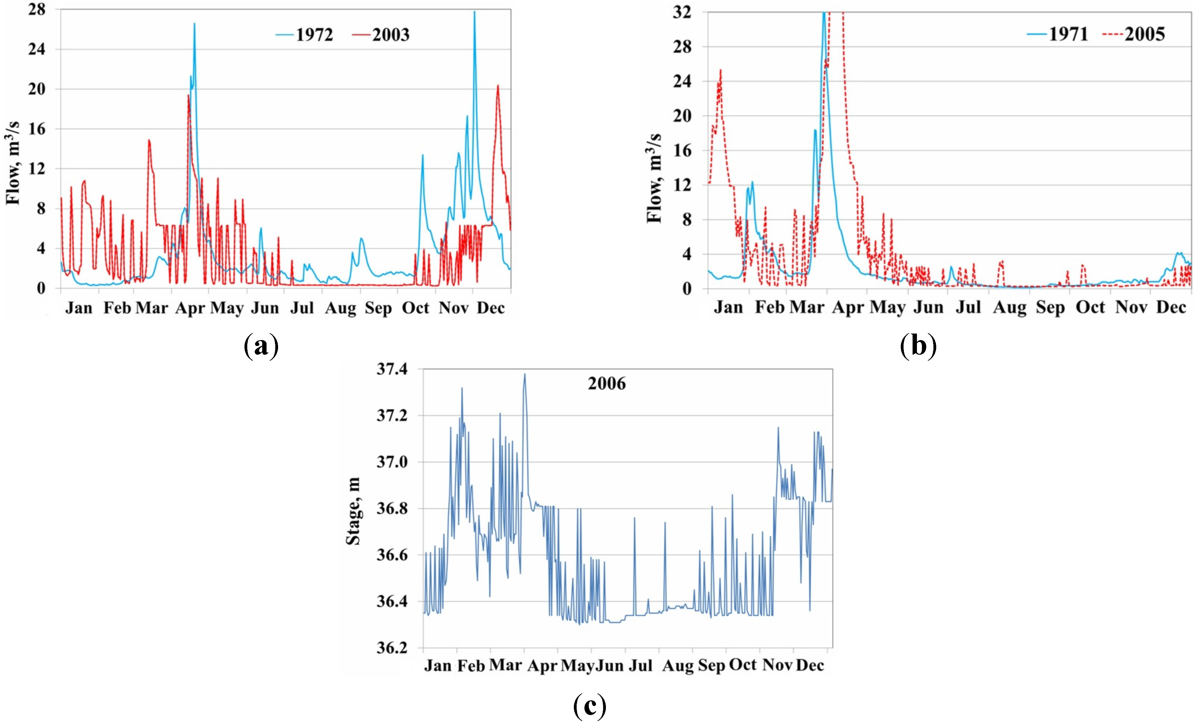
3.2. River Flow Alterations by Upstream Storage

To date, more than 90 SHP plants are operating in the country. Taking into account the fact that drawdown depth in SHP reservoirs is very limited (±0.1 m of NWL), they cannot be considered as highly dynamic water storage systems. Consequently, SHPs are unlikely to provide peak power because of the limited capacity of upstream storage volume.
Referring to Table 1 and Table 2, the indicators D and K were determined for the reservoir useful storage (drawdown depth of 1 m) and power storage (Figure 7). The latter corresponds to the depth h = 0.2 m and is exclusively used for the power generation.
Nearly half of the SHPs (42 out 90) can be viewed as run-of-river types, if the reservoir drawdown depth of 0.2 m designed for power generation is considered (water retention time in reservoir D0.2m < 2 h). For the SHPs under consideration, Angiriai and Vaitiekunai, this indicator ranges between 23 hours and 15 hours, respectively, and their magnitudes correspond to the pondage mode of operation (Table 1). By contrast, this indicator for the 100 MW Kaunas HP reservoir (A = 63.5 km2, h = 0.8 m or ±0.4 m of NWL) operating exclusively at peaking mode is 2 to 3 times bigger (D0.8m = 50 h).
Figure 7. Water retention indicators of SHP reservoirs. D (a) and K (b) determined for the reservoir useful and power storage. The subscript 0.2 m indicates a drawdown height of 0.2 m in reservoir.
Energies 08 07478 g007
According to the indicator K0.2m almost all reservoirs can be considered as run-of-river reservoirs, with a few exceptions. On an annual scale, water is renewed every day in the Angiriai reservoir and every half-day in the Vaitiekunai reservoir (K0.2m = 381 and 572, respectively). These indicators reflect the operations of reservoirs located on small or medium sized lowland rivers, because the reservoirs do not experience significant seasonal or shorter-term water level fluctuations due to relatively moderate river flow regimes.

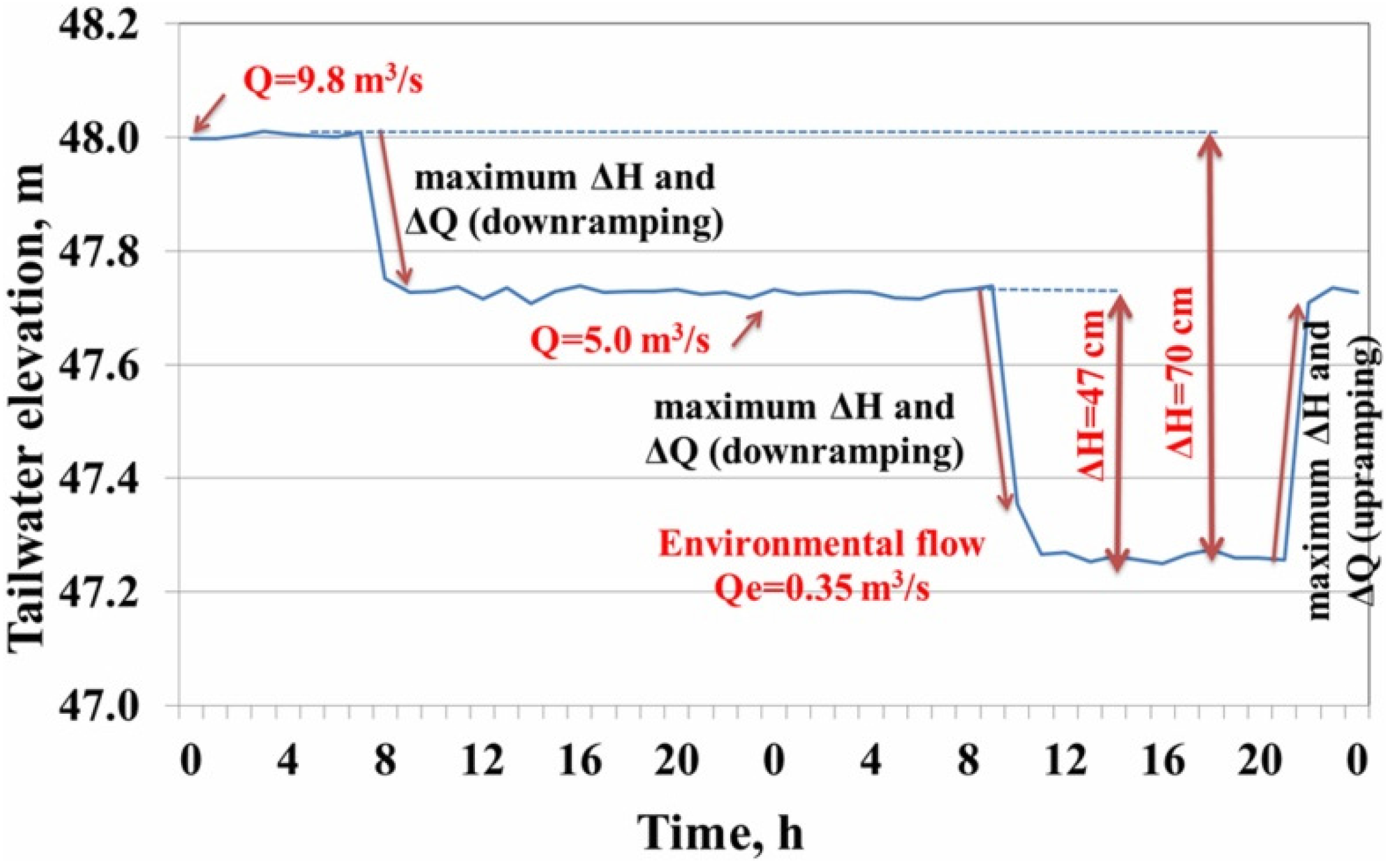
3.3. Flow (Stage) Ramping

3.3.1. Mechanics of Ramping

The primary type of turbine operations causing flow ramping downstream in the river reach is turbine start-up and shutdown, not a response to changes in electrical loads in Lithuania. Observations show that ramping occurs at irregular intervals during 24 hours or weekday periods that is different from the hydropeaking mode of operation, where constant flow is mostly observed at weekends. Ramping consequences are most crucial in the lean period of the river flow, especially when the inflow into an SHP reservoir is minimal. The main causes of flow ramping are as follows:
  • Operators, believing that they are producing more power are deliberately starting/shutting down turbines frequently during day/night periods for a certain number of hours. During the remaining time, turbines are operating at minimum flow or they can be completely stopped to comply with the prescriptions of instream flow. This mode of operation is inappropriate because energy output will be the same if turbines are operated at a reduced capacity but with stable patterns during 24 hours.
  • Turbines are not well adapted to the natural streamflow regime. This means that the design discharge of the turbines is too high, and control of the discharge flowing through the turbines is not flexible. In particular, this is evident for Angiriai SHP, which has a very high design discharge of propeller-type turbines (QT ≈ 2 Q0).
On the other hand, these artificial downstream flow (stage) fluctuations are due to the presence of an impoundment, and they cannot be completely avoided. Completely different geomorphological properties of the reservoir and the river channel downstream from the plant determine the significance of water level fluctuations. In other words, the upstream storage cross-sectional area is many times larger than that of downstream river (Figure 1). For instance, the drawdown depth of 1 cm in the Vaitiekunai reservoir results in an increase of 23 cm in the downstream water level (QT = 0.87 m3/s). Approximately the same amount of drawdown in the Juodeikiai reservoir (the Varduva river) incurs a rise in downstream water levels of 52 cm (QT = 2.42 m3/s). These findings were obtained during a low water season (the end of summer) when inflow into the reservoir was extremely minimal and no turbine was able to operate. It is absolutely clear that damping the range of water stage fluctuations is very problematic. Additionally, the requirement to maintain upstream storage water levels as stable as possible (±10 cm of NWL) is not an effective means of regulating the range of downstream stage fluctuations.

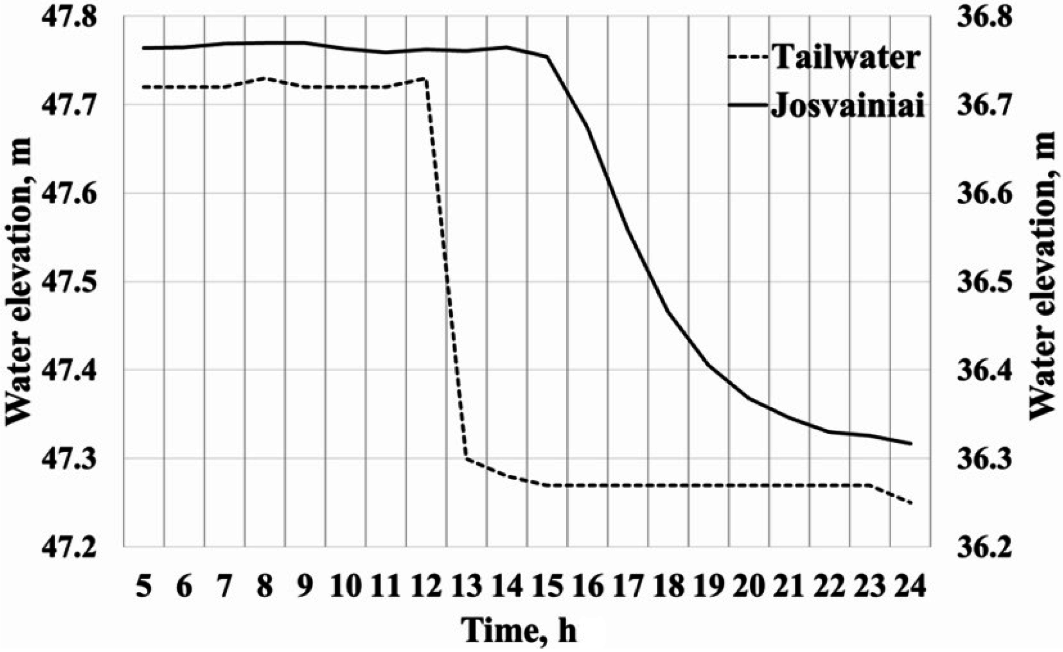
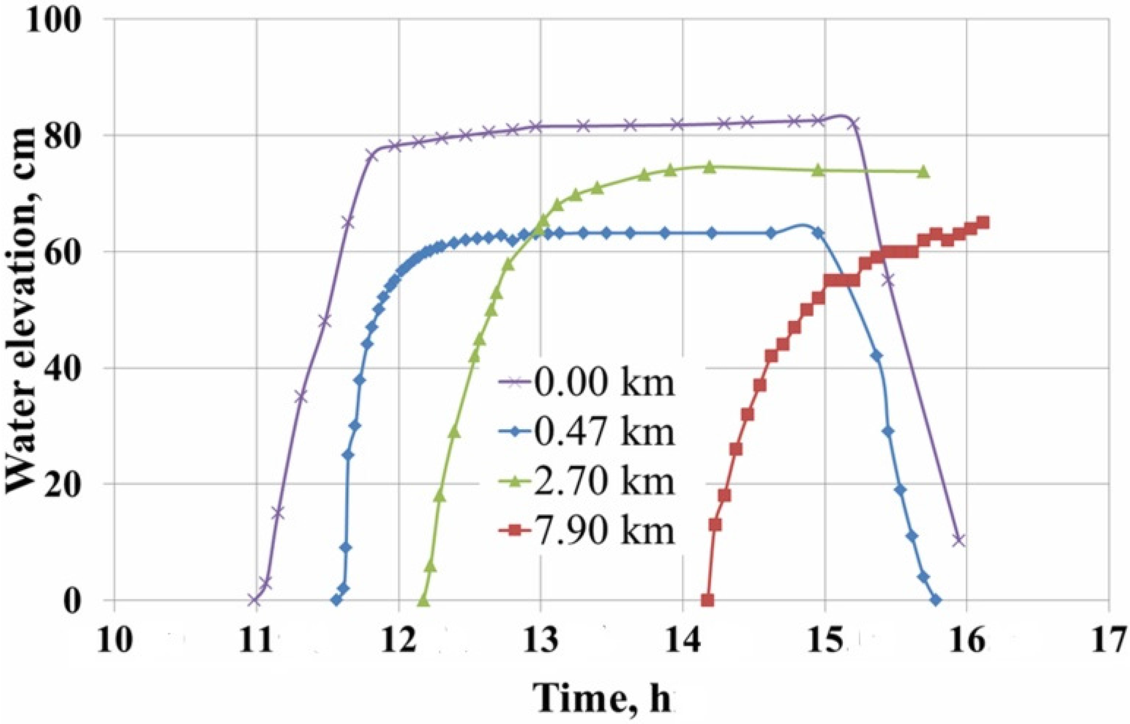
3.3.2. Downstream River Stage Fluctuations

The operation mode of Angiriai SHP obviously changes the river’s natural flow and stage variations, which were recorded 10 km downstream of the plant (Figure 8). 1971 and 1972 correspond to the years with the reservoir and 2003 and 2005 complemented with SHP. For the latter, a saw-toothed pattern is clearly seen. This hydroelectric facility is a pondage type (D0.2m = 23 h), although its hydrograph ramping has nothing to do with peak power demand.
Figure 8. Daily hydrographs (flow and stage) before the construction of Angiriai SHP (1971 (b), 1972 (a)) and under its operation (2003 (a), 2005 (b), 2006 (c)). Gauging station Susve at Josvainiai.
Energies 08 07478 g008
More obvious are the hourly flow and water level fluctuations downstream. For this SHP, the stage range can reach up to 70 cm within a 24 h period (Figure 9). For the country’s SHPs, the stage range at their tailwater varies between 10 and 70 cm, and for large, peaking Kaunas HP it can reach even 150 cm during a 24 h period [16,61]. This is because the turbines are not well adapted to the natural stream flow regime, which means that the design flow of the turbines is too high and the control of the discharge passing through the turbines is not flexible.
The ratio between turbine minimum flow and instream flow (QT/Qe) varies between 15 for Angiriai SHP and 1.4 for Vaitiekunai SHP. For comparison, this ratio in Swiss and Austrian rivers with operating hydropower facilities ranges from 2 to more than 50 [62]. Bain [32] reported extremely high ratios (maximum/minimum flows) for large hydropower facilities of 200 to 1000 (average of 166) in some rivers in the United States, Canada, Finland and France, and these rivers were classified as having moderate to severe alterations of aquatic ecosystems. Up-ramping and down-ramping stage rates (HR2) for Angiriai SHP are similar (25–30 cm/h), with slightly more intensive rising limbs.
Figure 9. Hourly tailwater level (H) fluctuations at Angiriai SHP. At the beginning, 2 turbines (QT = 9.8 m3/s) are working, then 1 turbine was shut down (QT = 5 m3/s) and finally both are shut down. Later, 1 turbine was started up again (3–4 March 2009). Inflow into the reservoir Q0 = 3.7 m3/s, HR1 = 1.33.
Energies 08 07478 g009
Open channel hydraulics and hydrological theory demonstrate that hydrograph is modified as water flows downstream a river channel [63,64,65]. It means that flow ramping attenuates as a function of the distance downstream from the turbines. However, this attenuation (for instance, stage range) over quite a long distance is not impressive, with a lagging time of approximately 4 hours (Figure 10).
Figure 10. Stage dynamic at the tailwater of Angiriai SHP after shutting down 1 turbine (QT = 5 m3/s, HR1 = 1.22) and 10 km downstream river at the Josvainiai gauging station. 10 May 2013. HR1 = 1.22.
Energies 08 07478 g010
The stage down-ramping rate at the power plant tailwater is 43 cm/hour, and at a distance of 10 km downstream it decreases to 7 cm/hour and approaches the natural hydrograph recession rate upper limit.
The same path was confirmed by a field experiment to determine the mechanics of travelling artificial flood wave downstream at the start-up and shut down of the turbines (Figure 11).
Figure 11. Stage hydrographs at different distances of the release of turbine water at Angiriai SHP. 18 August 2009, on the Susve River. Two turbines were started at a full capacity and shut down after 3 h. (Elevation not to datum).
Energies 08 07478 g011
It must be underlined that this was an unusual mode of turbine operation. After starting the turbines, the velocity in the tailwater was 1 m/s; later, due to significant channel resistance (vegetation, sinuosity, etc.) it was reduced to 0.8 m/s. As expected, the maximum stage up-ramping rate (HR2 = 90 cm/h) was recorded at the turbine water outlet—the tailrace. This is obvious because of a rapid increase in discharged flow by turbines (from 0 to 5.2 m3/s and very swiftly to 10.5 m3/s). At the second transect (0.47 km below the powerhouse), the up-ramping rate (HR2 = 90 cm/h) did not change, though it progressively lessened flowing downstream from the third and fourth transects (60 and 70 cm/h, respectively). The down-ramping rate was also significant—HR2 = 75 cm/h—at the second transect. Stage range diminished progressively through the river length from 80 cm to 60 cm, but its value was dependent on the channel geometry. This and other recently completed experiments on SHPs confirmed the initial hypothesis that the negative effects of turbine surge waves can be felt a long distance downstream the river. To mitigate this effect, turbine start-up and shutdown times should be extended as much as possible. Hydropower operations must begin and end with the turbine passing the least flow possible.
The analysis of historic flood records of the Susve River (natural river flow and pre-impoundment) reveals that the daily maximum stage rising is 6 cm/h and its recession is two times lower, 3 cm/h. Hourly rates are at least 1.5 times higher, approximately 9 and 5 cm/h, respectively. This bias is due to a smaller interval of measurements. Downstream from the Angiriai SHP, these estimates are exceeded at least 3 times. One important issue must be mentioned, which is that the frequency of natural floods is low compared with moderate artificial flooding caused almost daily by turbine operations.
Down-ramping rates of less than 5 cm/h are naturally observed after flood events in alpine rivers. Gentle flow ramping slower than 10 cm/h drastically decreases the stranding of juvenile fish [14]. An average value of 12–20 cm/h for the down-ramping rate is generally seen as an ecologically acceptable value [61]. Of course, rates are determined by channel geometry and hydraulic parameters, which vary temporally and spatially. Pools, side-channels, and gravel bars attenuate the ramping rate by storing water from higher flows and release this water gradually. Tributary inflow will attenuate the ramping rate and the ramping range.
The highest stage range magnitudes are observed for SHPs with high values of turbine design flow, mostly exceeding Q d T > (1.5…2.0)Q0, with unregulated turbines and minimal turbine numbers. However, the latter is seldom valid for the double regulated Kaplan and crossflow turbines, which are able to adapt well to the natural flow regime.

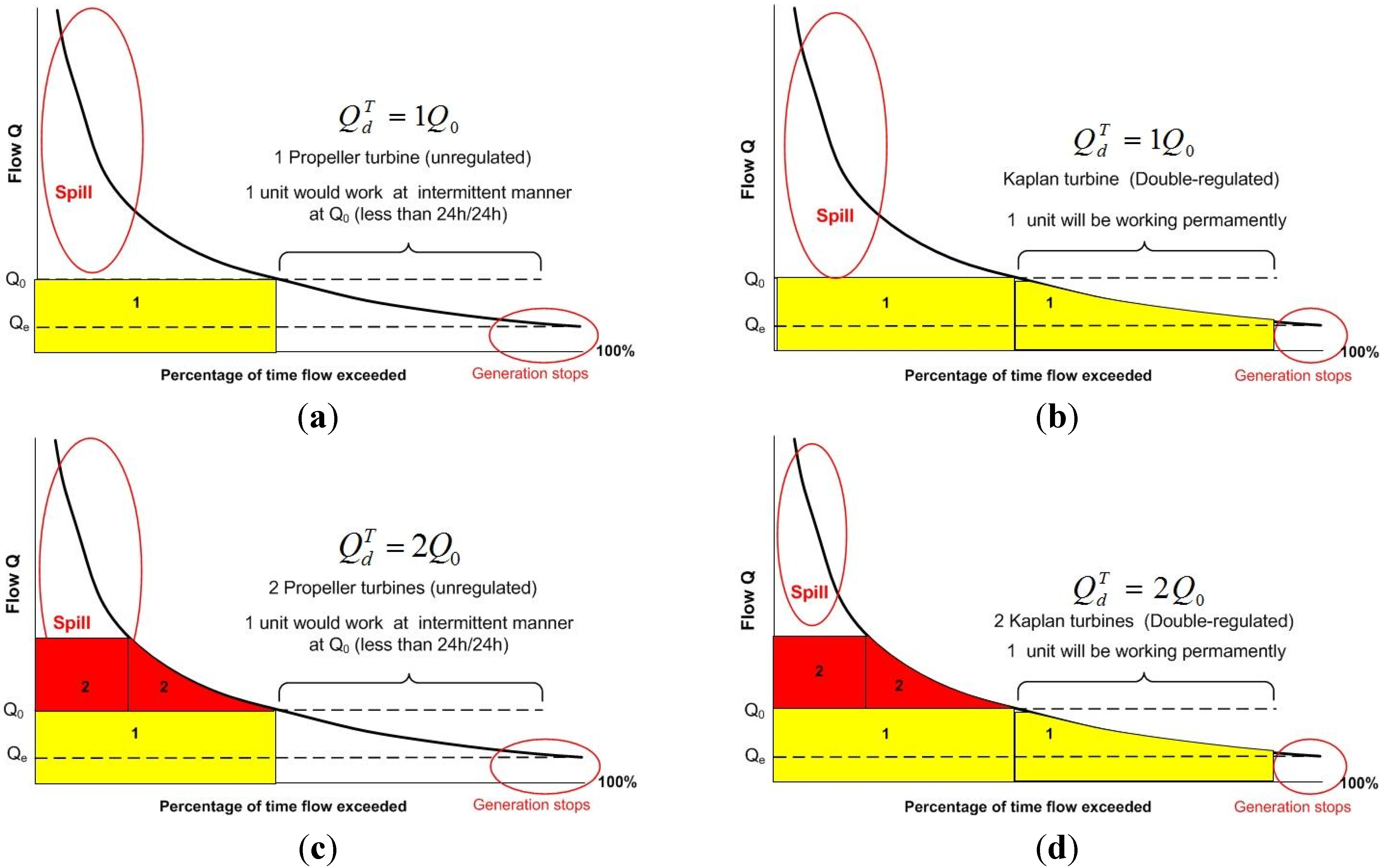
3.4. Assessment of Turbine Types with Regard to Possible Alterations of River Flow

It is convenient to present a river flow regime in the form of a flow duration curve (FDC), which was considered in the previous section. In hydropower engineering, the FDC serves as a basis for determining the number of turbines and the installed capacity. To preserve as possibly as natural river flow pattern and assure a reasonable use of water resources for power generation the area under this curve must be completely used by water discharged from turbines.
Figure 12. (a) 1 Propeller turbine, Q d T = 1Q0; (b) 1 Kaplan turbine, Q d T = 1Q0; (c) Two propeller turbines, Q d T = 2Q0; (d) Two Kaplan turbines, Q d T = 2Q0. Hypothetical FDC and its coverage by the propeller and Kaplan turbines (from 1 to 2 units). Q—daily flow; Q d T —design discharge of turbines; Q0—mean annual flow; Qe—environmental (instream) flow. Red and yellow indicate turbines working field.
Energies 08 07478 g012
However, for economic and technical considerations, neither the upper part (high water) nor the lower part (low water) of an FDC can be practically used (Figure 12). In practice, hydropower schemes generally have the greatest impacts on mid-range river flows and low flows [66]. A clear difference is seen between different types of turbines (Kaplan and propeller) and their number of “covering” FDC. The bigger the number of turbines and their flexibility to pass a larger range of flow through them, the better the coverage is. It is obvious that the Kaplan turbine (there might be other types as well) outperforms the propeller turbine (unregulated) in terms of using natural flows much larger than its range. The installed capacity of a plant, which is closely related to design discharge, cannot always play a definitive role; the number of turbines and their ability to adjust to a variety of river flows is much more important. As a result, the risk for intermittent modes of operation would be minimised (with some exceptions at the lower end of FDCs) and possible ramping avoided.
Typically, a hydropower developer chooses a design flow for the scheme that allows it to use a good proportion of the higher flows but also to continue to operate down to reasonably low flows so that output can be sustained for as much of the year as possible. In the UK, for low head schemes the common practice has been to use Q0 flow as the design flow [66]. For SHPs operating in Lithuania, the maximum design flow of turbines exceeds 1.5Q0. The more advanced and higher the turbine’s technical performance is, the more adaptive it will be to natural stream flow regimes (Table 7). The Kaplan double regulated turbine fits any river flow regime.
From the above, it can be concluded that the risk of emerging flow ramping is much greater in flashy rivers than in rivers with little variation in flow regime.
Table 7. Recommended turbine type taking into account river flow regime.
Turbine TypeDescription of Most Suitable River Flow Regime
Kaplan and propellerPropeller (unregulated)Only for low variation in flow regime, not suitable for flashy rivers. This means that the low flow has a considerable proportion of the mean flow. The FDC must have a very flat slope. *
Kaplan (single regulated)Moderate variation in flow regime
Kaplan (double regulated)Any variation in flow regime (any shape of FDC)
FrancisOnly for low variation in flow regime. Not suitable for streams with initially steeply sloped FDCs
Cross-flow (Ossberger, Banki-Michell, Cink)Any variation in flow regime
* A good indication for variation in river flow regimes can be given by the shape of the FDC (for daily discharges), which can be expressed numerically.

4. Conclusions

(1)
The basic statistical test allows us to conclude that no significant trends were detected in the long-term hydrological data series and that the employed data represents necessary hydrological cycles.
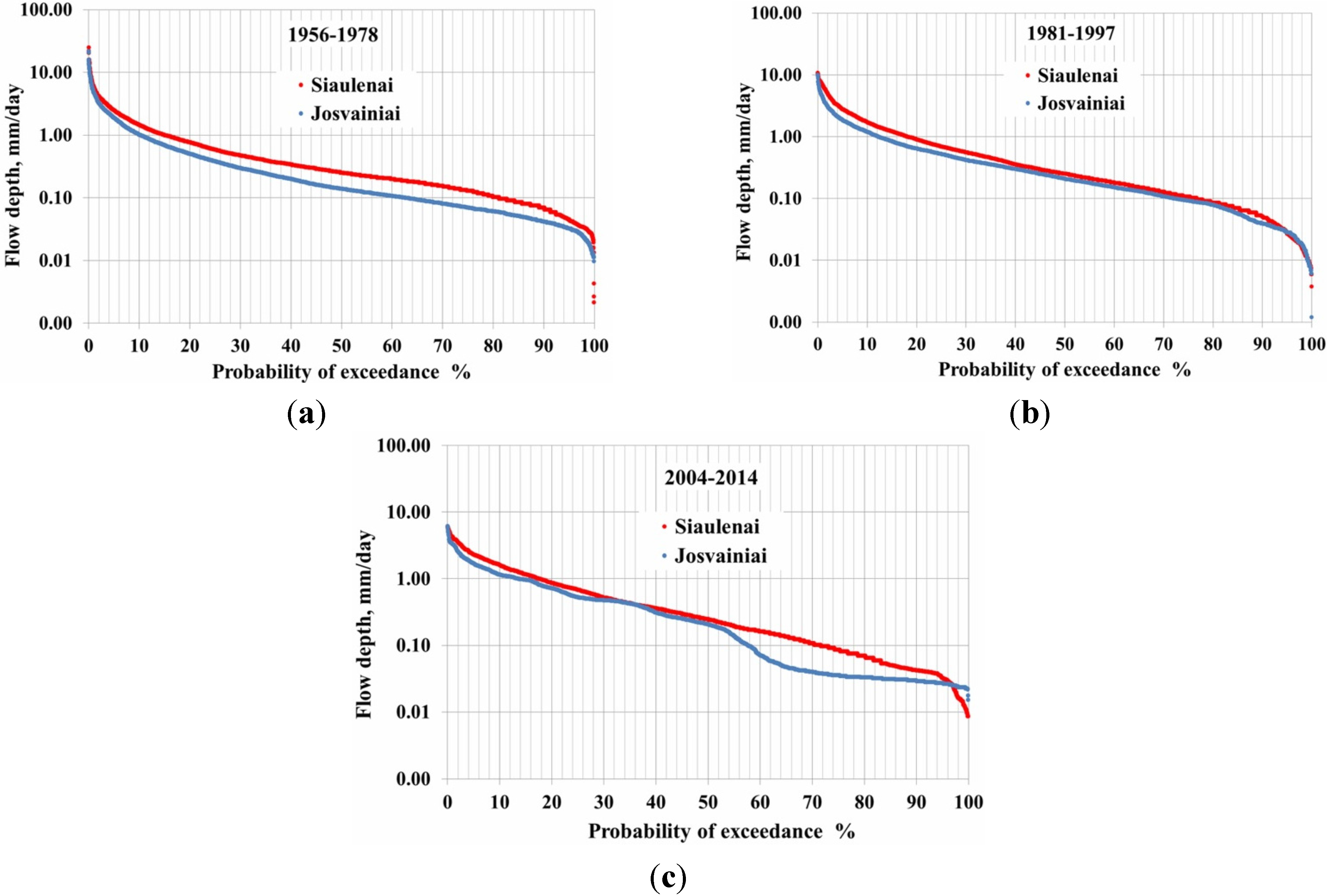
(2)
The FDC derived from long-term records consisting of pre-post impoundment and SHP development does not markedly differ in the first and second period, but differs in the third period, especially the lower part of the curve, this points to possible impact of the Angiriai SHP.
(3)
Water retention time (D and K) is a simple and good indicator to evaluate the significance of probable impacts of an impoundment on river flow. Despite this fact, the proposed threshold values need to be based more scientifically.
(4)
Downstream river flow (stage) ramping is an environmental issue for large hydro, and small hydropower alike. The operation of small run-of-river power plants that do not necessarily follow energy peak demand could possibly result in this negative phenomenon.
(5)
More intensive fluctuations in the downstream river flow and stage can be observed in SHPs with high turbine design flows, unregulated types of turbines and a low number of turbines.
(6)
When an SHP is not intended for operations covering peak energy demand, its design turbine flow should not exceed the mean annual river discharge. There are currently a large number of advanced turbines available. The turbines have a wide range of capacities, there are also advances in turbine design (e.g., double regulated or cross-flow). These features will allow for adapting higher values of design flows with a minimum risk of flow ramping.
(7)
By applying simple turbine operational measures—step-wise turbine start up and shut-down together with varying their number and capacities during 24 h—river flow ramping rates can be substantially alleviated.
(8)
Recommended turbine types are most suitable for a particular natural flow regime. However, total avoidance of downstream hydrograph ramping is not possible without applying structural measures (involving physical constructions) for run-of-river projects with impoundments.

Acknowledgments

The authors would like to thank Kelly Kibler of University of Central Florida and the anonymous reviewer for investing their spare time in reviewing this manuscript, for their valuable comments and suggestions in order to help improve this manuscript. Some information for this paper was used from the RESTOR Hydro project (Intelligent Energy-Europe Program, 2012–2015, coordinated by the European Small Hydropower Association) and past and ongoing studies funded by the Lithuanian Environment Agency and the Research Council of Lithuania.

Author Contributions

Petras Punys designed this research and gave the whole guidance; Antanas Dumbrauskas and Gitana Vyčienė largely wrote pre- and post-hydrological changes, Egidijus Kasiulis and Linas Šilinis collected all the data, carried out calculations, result display and analysis. All authors read and approved the final manuscript.

Conflicts of Interest

The authors declare no conflict of interest.

Nomenclature

SHP
small hydropower plant
HP
hydropower plant
Q0
mean flow
QT
turbine discharge
QTd
design flow of turbine
Qe
environmental (instream) flow
D
water retention time in a reservoir (reservoir filling period)
K
water retention indicator related to water retention time in a reservoir
FDC
mean daily flow duration curve
RoR
run-of-river (HP operation mode)
GS
river flow and stage gauging station
h
drawdown depth of a reservoir needed for power generation
WL, NWL
water level, reservoir normal water level

References

  1. Jia, J.; Punys, P.; Ma, J. Hydropower. In Handbook of Climate Change Mitigation; Springer Science: New York, NY, USA, 2012; pp. 1357–1401. [Google Scholar]
  2. Elizabeth Stewart Hands and Associates (ESHA). The European Small Hydropower Association. Available online: http://www.esha.be/ (accessed on 6 March 2015).
  3. Punys, P.; Pelikan, B. Review of small hydropower in the new member states and candidate countries in the context of the enlarged European Union. Renew. Sustain. Energy Rev. 2007, 11, 1321–1360. [Google Scholar] [CrossRef]
  4. Arcadis. Hydropower Generation in the Context of the EU WFD. Report to EC DG Environment. Project No 11418. 2011. Available online: http://www.arcadis.de/Content/ArcadisDE/docs/projects/11418_WFD_HP_final_110516.pdf (accessed on 10 June 2015).
  5. Elizabeth Stewart Hands and Associates (ESHA). Small Hydropower Roadmap. Report. Condensed Research Data for EU-27. The Stream Map Project. 2012. Available online: http://streammap.esha.be/fileadmin/documents/Press_Corner_Publications/SHPRoadmap_FINAL_Public.pdf (accessed on 9 June 2015).
  6. Reihan, A.; Loigu, E. Small hydropower in Estonia—Problems and perspectives. In Proceedings of the European Conference on Impacts of Climate Change on Renewable Energy Sources, Reykjavik, Iceland, 5–9 June 2006.
  7. Abbasi, T.; Abbasi, S.A. Small hydro and the environmental implications of its extensive utilization. Renew. Sustain. Energy Rev. 2011, 5, 2134–2143. [Google Scholar] [CrossRef]
  8. Vaikasas, S.; Bastiene, N.; Pliuraite, V. Impact of small hydropower plants on physicochemical and biotic environments in flatland riverbeds of Lithuania. J. Water Secur. 2015, 1, 1–13. [Google Scholar] [CrossRef]
  9. Kubecka, J.; Matena, J.; Hartvich, P. Adverse ecological effects of small hydropower stations in the Czech Republic: 1. Bypass plants. Regul. Rivers Res. Manag. 1997, 13, 101–113. [Google Scholar] [CrossRef]
  10. Fu, X.; Tang, T.; Jiang, W.; Li, F.; Wu, N.; Zhou, S.; Cai, Q. Impacts of small hydropower plants on macroinvertebrate communities. Acta Ecol. Sin. 2008, 28, 45–52. [Google Scholar]
  11. Kibler, K.M.; Tullos, D.D. Cumulative biophysical effects of small and large hydropower development, Nu River, China. Water Resour. Res. 2013. [Google Scholar] [CrossRef]
  12. European Commission. Directive 2000/60/EC of the European Parliament and of the Council of 23 October 2000 establishing a framework for Community action in the field of water policy. Off. J. Eur. Communities 2000, L327, 1–73. [Google Scholar]
  13. European Commission. Common Implementation Strategy for the Water Framework Directive. WFD and Hydro-Morphological Pressures Policy Paper. Focus on Hydropower, Navigation and Flood Defense Activities. Recommendations for Better Policy Integration. Available online: http://www.sednet.org/download/Policy_paper_WFD_and_Hydro-morphological_pressures.pdf (accessed on 6 March 2015).
  14. Meile, T.; Boillat, J.L.; Schleiss, A.J. Hydropeaking indicators for characterization of the Upper-Rhone, river in Switzerland. Aquat. Sci. 2011, 73, 171–182. [Google Scholar] [CrossRef]
  15. Smokorowski, K.E.; Metcalfe, R.A.; Jones, N.E.; Marty, J.; Niu, S.; Pyrce, R.S. Flow management: Studying ramping rate restrictions. Hydro Rev. 2009, 28, 68–87. [Google Scholar]
  16. Aplinkos apsaugos agentūra. Aplinkosauginių rekomendacijų hidroelektrinių neigiamam poveikiui sumažinti parengimas (Report to EPA on environmental measures to reduce the negative impact of hydropower plants). Aplinkos apsaugos agentūra: Vilnius, Lietuva, 2010; p. 316. (In Lithuanian) [Google Scholar]
  17. Richter, B.D.; Baumgartner, J.V.; Powell, J.; Braun, D.P. A method for assessing hydrologic alteration within ecosystems. Conserv. Biol. 1996, 10, 1163–1174. [Google Scholar] [CrossRef]
  18. Olden, J.D.; Poff, N.L. Redundancy and the choice of hydrologic indices for characterizing streamflow regimes. River Res. Appl. 2003, 19, 101–121. [Google Scholar] [CrossRef]
  19. Magilligan, F.J.; Nislow, K.H. Changes in hydrologic regime by dams. Geomorphology 2005, 71, 61–78. [Google Scholar] [CrossRef]
  20. Rueda, F.; Moreno-Ostos, E.; Armengol, J. The residence time of river water in reservoirs. Ecol. Model. 2006, 191, 260–274. [Google Scholar] [CrossRef]
  21. Delhez, E.J.M.; de Brye, B.; de Brauwere, A.; Deleersnijder, E. Residence time vs. influence time. J. Mar. Syst. 2014, 4, 185–195. [Google Scholar] [CrossRef]
  22. Brune, G.M. The trap efficiency of reservoirs. Trans. Am. Geophys. 1953, 34, 407–418. [Google Scholar] [CrossRef]
  23. Kondolf, G.M.; Batalla, R.J. Hydrological effects of dams and water diversions on rivers of mediterranean-climate regions: Examples from California. In Catchment Dynamics and River Processes: Mediterranean and Other Climate Regions Developments in Earth Surface Processes; Batalla, R.J., Ed.; Elsevier: Amsterdam, The Netherland, 2005; pp. 197–211. [Google Scholar]
  24. Unipede-Eurelectric. Statistical Terminology Employed in the Electricity Supply Industry; Unipede-Eurelectic: Brussels, Belgium, 1991. [Google Scholar]
  25. Punys, P.; Sabas, G. Small hydropower operations and natural hydrological regime. Case study in Lithuania. In Proceedings of the Hidroenergia 2012: International Congress and Exhibition on Small Hydropower, Wroclaw, Poland, 23–26 May 2012.
  26. Hursie, U. Designation of HMWB & GEP. In Proceedings of the Workshop Water Framework Directive and Heavily Modified Water Bodies, Brüssel, Belgium, 12–13 March 2009.
  27. Warnick, C.C. Hydropower Engineering; Prentice-Hall: Englewood Cliffs, NJ, USA, 1984. [Google Scholar]
  28. American Society of Civil Engineers (ASCE). Civil Engineering Guidelines for Planning and Designing Hydroelectric Developments; Small Scale Hydro. ASCE: New York, NY, USA, 1989; Volume 4, p. 333. [Google Scholar]
  29. RETScreen® International. RETScreen® Engineering & Cases Textbook. Small Hydro Project Analysis Chapter. Natural Resources Canada. 2004. Available online: http://www.retscreen.net/ (accessed on 11 June 2015).
  30. Douglas, T. “Green” hydro power understanding impacts, approvals, and sustainability of run-of-river independent power projects in British Columbia. Watershed Watch Salmon Society. Available online: http://www.watershed-watch.org/publications/files/Run-of-River-long.pdf (accessed on 6 March 2015).
  31. World Atlas & Industry Guide, 2013. In The International Journal on Hydropower & Dams; Aqua Media International Ltd.: Wallington, UK, 2013.
  32. Bain, M.B. Report: Hydropower Operations and Environmental Conservation: St. Marys River, Ontario and Michigan; International Lake Superior Board of Control: Conrnwall, ON, Canada; Cicinnati, OH, USA, 2007. [Google Scholar]
  33. Hunter, M.A. Hydropower Flow Fluctuations and Salmonids: A Review of the Biological Effects, Mechanical Causes and Options for Mitigation; Report No.119; State of Washington, Department of Fisheries: Washington, DC, USA, 1992. [Google Scholar]
  34. Harpman, D.A. Assessing the short-run economic cost of environmental constraints on hydropower operations at Glen Canyon Dam. Land Econ. 1999, 75, 390–401. [Google Scholar] [CrossRef]
  35. Tuhtan, J.A.; Noack, M.; Wieprecht, S. Estimating stranding risk due to hydropeaking for juvenile European grayling considering river morphology. KSCE J. Civil Eng. 2012, 16, 197–206. [Google Scholar] [CrossRef]
  36. Schmutz, S.; Bakken, T.H.; Friedrich, T.; Greimel, F.; Harby, A.; Jungwirth, M. Response of fish communities to hydrological and morphological alterations in hydropeaking rivers of Austria. River Res. Appl. 2014. [Google Scholar] [CrossRef]
  37. Charmasson, J.; Zinke, P. Mitigation Measures against hydropeaking Effects. A Literature Review; Report No. TR A7192-Unrestricted; Stiftelsen for Industriell og Teknisk Forskning (SINTEF): Trondheim, Norway, 2011. [Google Scholar]
  38. Meile, T. Hydropeaking on Watercourses. EAWAG News 61e. November 2006, pp. 28–29. Available online: http://www.eawag.ch/medien/publ/eanews/archiv/news_61/en61e_meile.pdf (accessed on 15 March 2015).
  39. Baumann, P.; Klaus, I. Conséquences Ecologiques des Eclusées. Etude Bibliographique; Informations concernant la pêche No 75; L'Office Fédéral de l'Environnement, des Forêts et du Paysage (OFEFP): Berne, Switzerland, 2003; p. 116. (In French) [Google Scholar]
  40. Water Framework Directive & Hydropower. Key Conclusions. Common Implementation Strategy Workshop: Berlin, Germany, 4–5 June 2007. Available online: http://www.ecologic-events.de/hydropower/documents/key_conclusions.pdf (accessed on 6 March 2015).
  41. Smokorowski, K.E.; Metcalfe, R.A.; Finucan, S.D.; Jones, N.; Marty, J.; Power, M. Ecosystem level assessment of environmentally based flow restrictions for maintaining ecosystem integrity: A comparison of a modified peaking vs. unaltered river. Ecohydrology 2011, 4, 791–806. [Google Scholar] [CrossRef]
  42. Jager, H.I.; Bevelhimer, M.S. How run-of-river operation affects hydropower generation and value. Environ. Manag. 2007, 40, 1004–1015. [Google Scholar] [CrossRef] [PubMed]
  43. Haas, N.A.; O’Connor, B.L.; Hayse, J.W.; Bevelhimer, M.S.; Endreny, T.A. Analysis of daily peaking and run-of-river operations with flow variability metrics, considering subdaily to seasonal time scales. JAWRA J. Am. Water Resour. Assoc. 2014, 50, 1622–1640. [Google Scholar] [CrossRef]
  44. Vaikasas, S.; Poškus, V. HE turbinų įjungimo sukeliamo potvynio bangos žemutiniame bjefe tyrimai (The investigation of HP turbines switch impact in river lower reaches). Vandens Inž. (Water Manag. Eng.) 2009, 35, 103–109. (In Lithuanian) [Google Scholar]
  45. Niu, S.; Insley, M. On the economics of ramping rate restrictions at hydro power plants: Balancing profitability and environmental costs. Energy Econ. 2013, 9, 39–52. [Google Scholar] [CrossRef]
  46. Heller, P.; Schleiss, A. Aménagements hydroélectriques fluviaux à buts multiples: Résolution du marnage artificiel et conséquences sur les objectifs écologique, énergétique et social. Houille Blanch. 2011, 6, 34–41. (In Lithuanian) [Google Scholar] [CrossRef]
  47. Ribi, J.; Boillat, J.; Schleiss, A. Flow Exchange between a Channel and a Rectangular Embayment Equipped with a Diverting Structure. 2010. Available online: http://infoscience.epfl.ch/record/151681 (accessed on 2 January 2015).
  48. Gostner, W.; Lucarelli, C.; Theiner, D.; Kager, A.; Premstaller, G.; Schleiss, A.J. A holistic approach to reduce negative impacts of hydropeaking. In Proceedings of the International Symposium on Dams and Reservoirs under Changing Challenges—79th Annual Meeting of ICOLD—Swiss Committee on Dams, Lucerne, Switzerland, 1 June 2011.
  49. Fishers and Oceans Canada. Flow Ramping Study. Study of Ramping Rates for Hydropower Developments; Report No. Va103-79/2-1; Fisheries and Oceans Canada, Knight Piésold Consulting: Vancouver, BC, Canada, 2005. [Google Scholar]
  50. Gailiušis, B.; Kriaučiūnienė, J. Runoff changes in the Lithuanian rivers due to construction of water reservoirs. In Proceedings of the Rural development 2009: The 4th International Scientific Conference, Akademija, Kaunas Region, Lithuania, 15–17 October 2009.
  51. Ždankus, N.; Vaikasas, S.; Sabas, G. Impact of a hydropower plant on the downstream reach of a river. J. Environ. Eng. Landsc. Manag. 2008, 16, 128–134. [Google Scholar] [CrossRef]
  52. Ždankus, N.; Sabas, G. The influence of anthropogenic factors to Lithuanian rivers flow regime. In Proceedings of the 6th International Conference Environmental Engineering, Rome, Italy, 26–27 May 2005; pp. 515–522.
  53. Vaikasas, S.; Palaima, K.; Pliuraite, V. Influence of hydropower dams on the state of macroinvertebrates assemblages in the Virvyte river, Lithuania. J. Environ. Eng. Landsc. Manag. 2013, 21, 305–315. [Google Scholar] [CrossRef]
  54. Gailiušis, B.; Jablonskis, J.; Kovalenkovienė, M. Lietuvos Upės: Hidrografija ir Nuotėkis Monografija (Lithuanian Rivers: Hydrography and Runoff); Lietuvos energetikos institutas: Kaunas, Lietuva, 2001; p. 791. (In Lithuanian) [Google Scholar]
  55. Dumbrauskas, A.; Larsson, R. The Influence of Farming on Water Quality in the Nevėzis Basin. Environ. Res. Eng. Manag. 1997, 2, 48–55. [Google Scholar]
  56. International Commission on Large Dams (ICOLD). Available online: http://www.icold-cigb.org/ (accessed on 15 March 2015).
  57. Ye, S.; Yaeger, M.; Coopersmith, M.; Cheng, L.; Sivapalan, M. Exploring the physical controls of regional patterns of flow duration curves—Part 2: Role of seasonality, the regime curve, and associated process controls. Hydrol. Earth Syst. Sci. 2012, 16, 4447–4465. [Google Scholar] [CrossRef]
  58. The Nature Conservancy. Indicators of Hydrologic Alteration Version 7.1—User’s Manual. Available online: https://www.conservationgateway.org/Files/Pages/indicators-hydrologic-altaspx47.aspx (accessed on 6 March 2015).
  59. Gore, J.A. The Restoration of Rivers and Streams: Theories and Experience; Butterworth/Ann: Arbor, MI, USA, 1985. [Google Scholar]
  60. Sauterleute, J.; Charmasson, J. Characterisation of rapid fluctuations of flow and stage in rivers in consequence of hydropeaking. In Proceedings of the 9th International Symoposium on Ecohydraulics, Viena, Austria, 17–21 September 2012.
  61. Sabas, G. Analysis of hydropower plant influence to the river hydrological and hydraulic regimes. In Proceedings of the 6th International Conference Environmental Engineering, Vilnius, Lithuania, 26–27 May 2005.
  62. Kraftwerksbedingter Schwall und Sunk. Eine Standortbestimmung, Im Auftrag des Schweizerischen Wasserwirtschaftsverbands; ETH Zürich: Lausanne, Switzerland, 2006. (In Lithuanian)
  63. Chow, V.T. Open-Channel Hydraulics; McGraw-Hill: New York, NY, USA, 1959. [Google Scholar]
  64. Handbook of Hydrology; Maidment, D.R. (Ed.) McGraw-Hill: New York, NY, USA, 1993.
  65. Shaw, E.M.; Beven, K.J.; Chappell, N.A.; Lamb, R. Hydrology in Practice, 4th ed.; CRC Press, Taylor & Francis Group: New York, NY, USA, 2010. [Google Scholar]
  66. Environment Agency (EA). The environmental assessment of proposed low head hydro power developments. In Good Practice Guidelines Annex to the Environment Agency Hydropower Handbook; EA: Rotherham, UK, August 2009. [Google Scholar]

