Article

A Multi-Objective Optimization Framework for Offshore Wind Farm Layouts and Electric Infrastructures

1
DC systems, Energy conversion & Storage Group, Delft University of Technology, Mekelweg 4, Delft 2628 CD, The Netherlands
2
Department of Industrial Technologies, Universidad de Talca, Talca 3340000, Chile
3
CITCEA-UPC, Carrer de Jordi Girona, 31, Barcelona 08034, Spain
4
ECN, Westerduinweg 3, Petten 1755 LE, The Netherlands
5
Centrum Wiskunde & Informatica, Science Park 123, Amsterdam 1098 XG, The Netherlands
*
Author to whom correspondence should be addressed.
Submission received: 2 November 2015 / Revised: 1 March 2016 / Accepted: 4 March 2016 / Published: 18 March 2016

Abstract

:
Current offshore wind farms (OWFs) design processes are based on a sequential approach which does not guarantee system optimality because it oversimplifies the problem by discarding important interdependencies between design aspects. This article presents a framework to integrate, automate and optimize the design of OWF layouts and the respective electrical infrastructures. The proposed framework optimizes simultaneously different goals (e.g., annual energy delivered and investment cost) which leads to efficient trade-offs during the design phase, e.g., reduction of wake losses vs collection system length. Furthermore, the proposed framework is independent of economic assumptions, meaning that no a priori values such as the interest rate or energy price, are needed. The proposed framework was applied to the Dutch Borssele areas I and II. A wide range of OWF layouts were obtained through the optimization framework. OWFs with similar energy production and investment cost as layouts designed with standard sequential strategies were obtained through the framework, meaning that the proposed framework has the capability to create different OWF layouts that would have been missed by the designers. In conclusion, the proposed multi-objective optimization framework represents a mind shift in design tools for OWFs which allows cost savings in the design and operation phases.

1. Introduction

Currently the offshore wind industry is aiming at reducing its cost of energy (COE) (M€/MWh) to breach the 100 €/MWh barrier as soon as 2020 [1,2,3,4,5,6] from the current 163 €/MWh [7]. Although the technologies used in offshore wind farms (OWFs) have greatly improved, the COE generated offshore is yet not competitive [8]. In fact, electricity generated offshore is currently approximately 50% more expensive when compared to onshore wind generation [9]. 
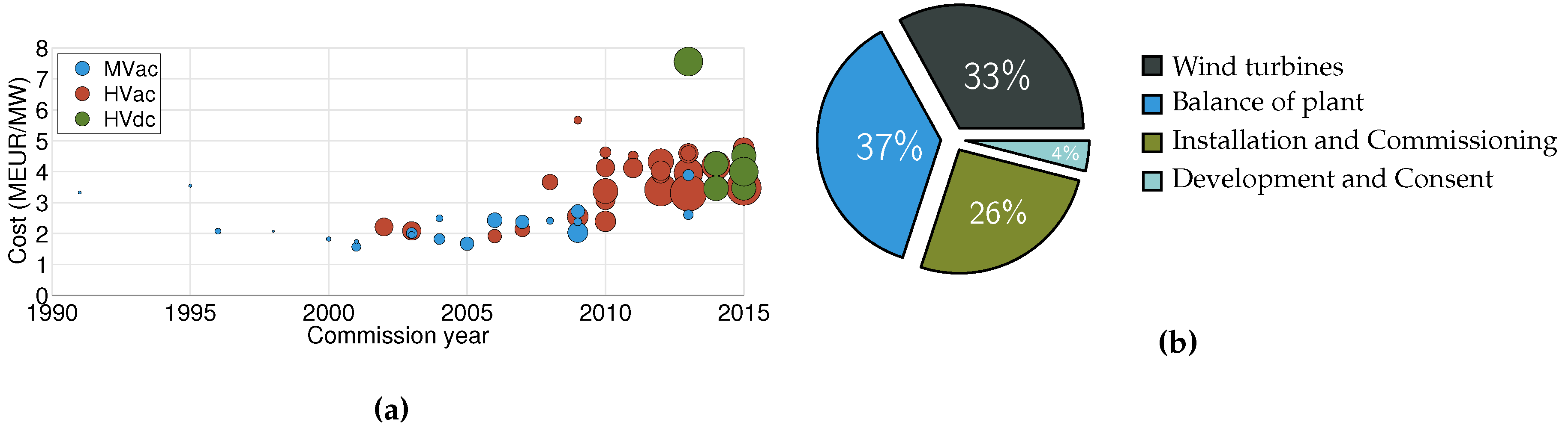
Figure 1a demonstrates that the cost of power (COP) (M€/MW) installed of OWFs has increased since the initial project and has not reduced in the last years [10,11].
There are different measures that can decrease the costs of the energy generated offshore [2,3,4,5,
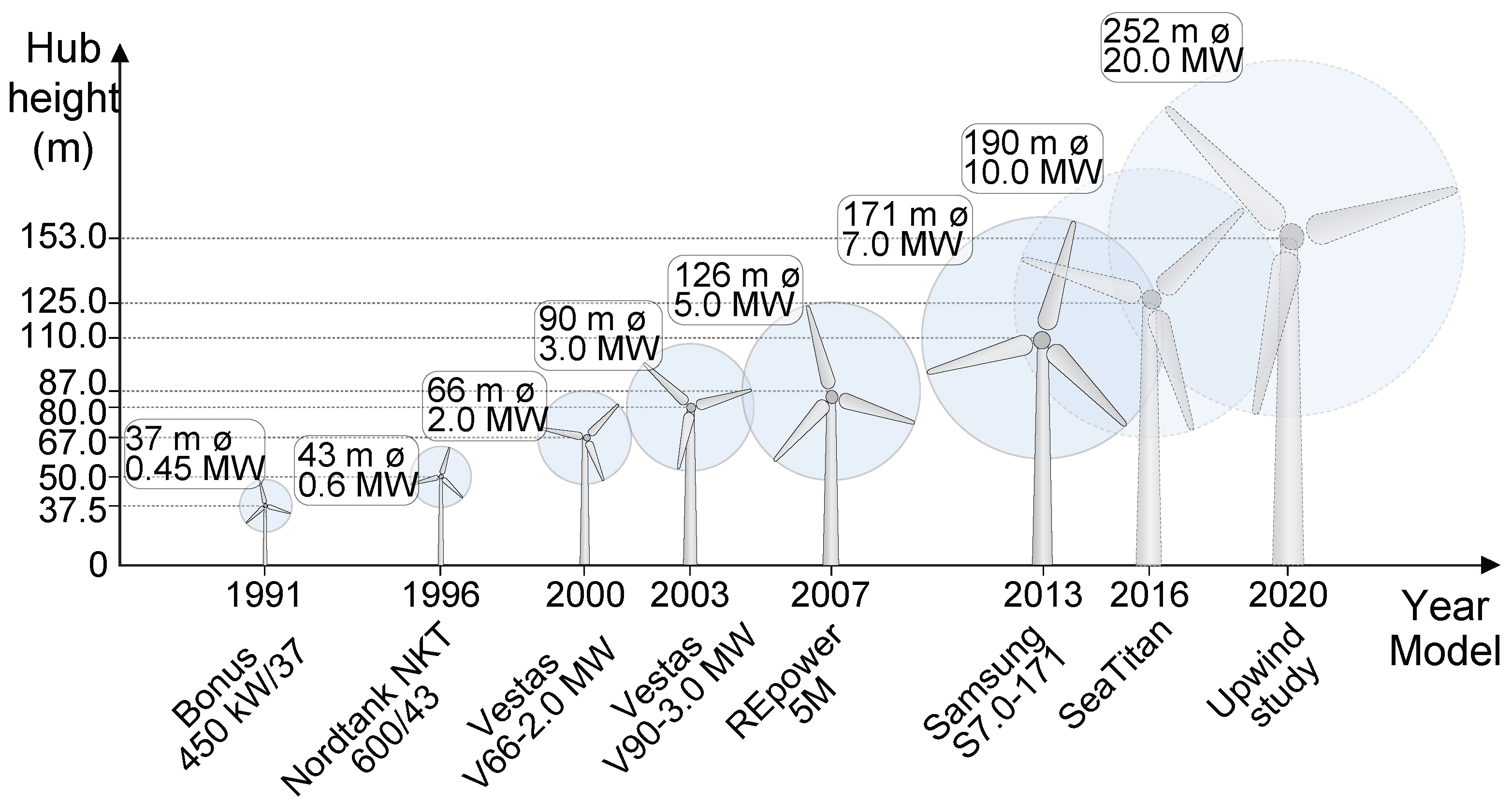
6]. Key factors are, for example, exploitation of economies of scale and greater standardization, introduction of turbines with higher rated power and reliability and greater activity at the front end engineering and design (FEED) phase.
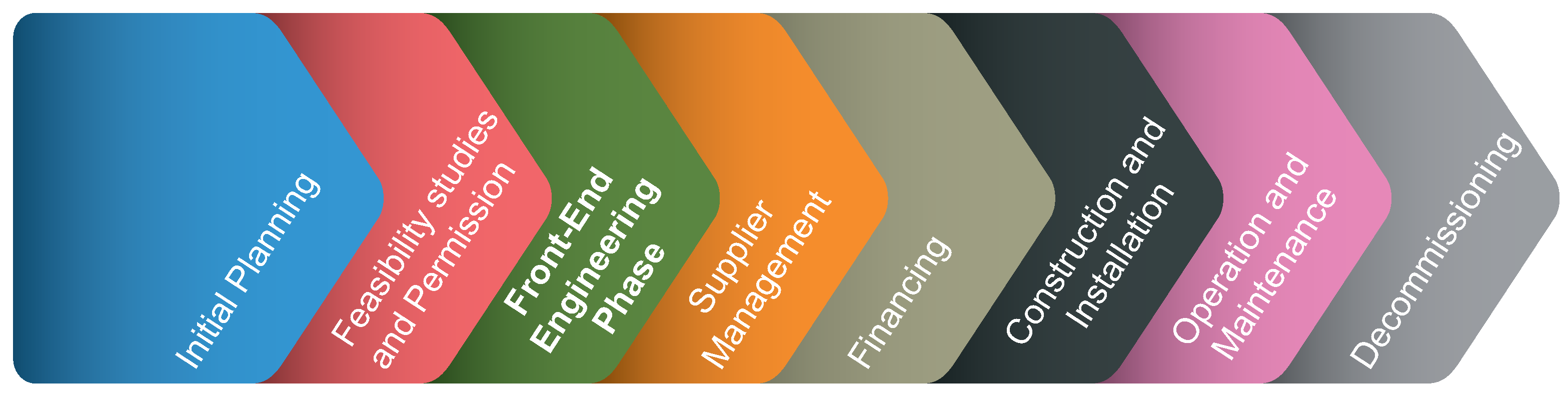
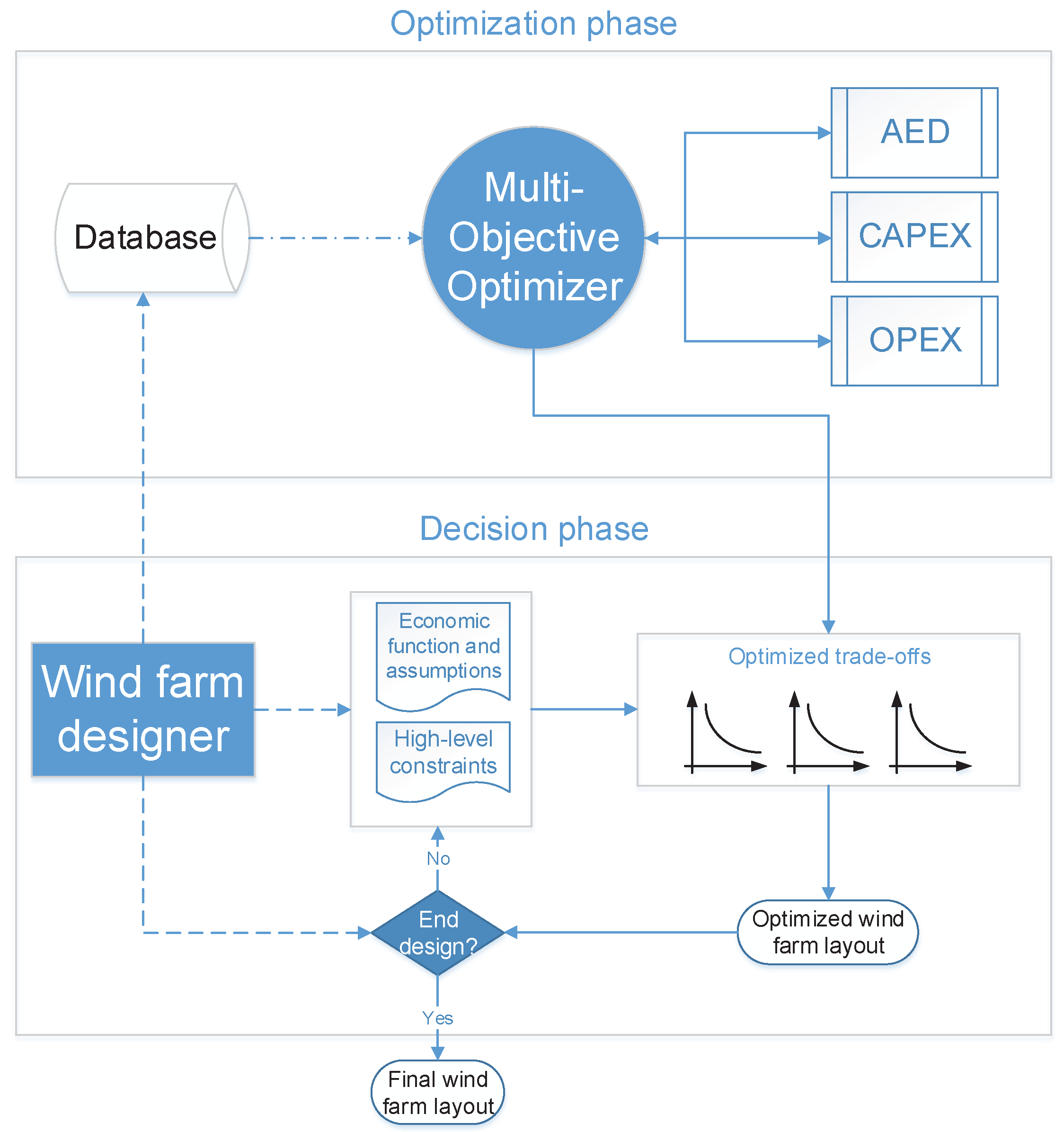
The design phase of an OWF is performed during the FEED phase (see Figure 2), after the initial feasibility studies have been done and permission has been granted, and before final investment decisions are made [2,14]. FEED studies allow wind farm developers to make a pre-selection of economically viable design concepts and the respective key components [3]. During the FEED phase, decisions have not yet been made regarding the number of turbines [15,16], the support structures that will be used or the number of substations that will be built [15,16]. In this phase, several layout concepts are preliminary designed, and although the final wind farm layout will be based on these designs, it may still differ considerably [15].
Several aspects have increased the need for a broader activity at the FEED stage [3]. The development phase of OWFs is time consuming due to the time needed to manually create several designs and the necessary cable routing [18,19,20]. In fact, circa 4% of the total capital expenditure (CAPEX) of an OWF are allocated to the development phase (see Figure 1b), in which all the components and technologies that lead to an optimized and feasible system must be assessed [13,21]. Recent OWFs occupy larger areas, which often have variable water depth and seabed conditions [22] and are situated further from shore [22], leading to more complex constraints and design challenges on the grid connection. Finally, the large number of wind turbines leads to complex collection systems, which need to be carefully assessed to achieve wind farm layouts with higher efficiencies [2]. 
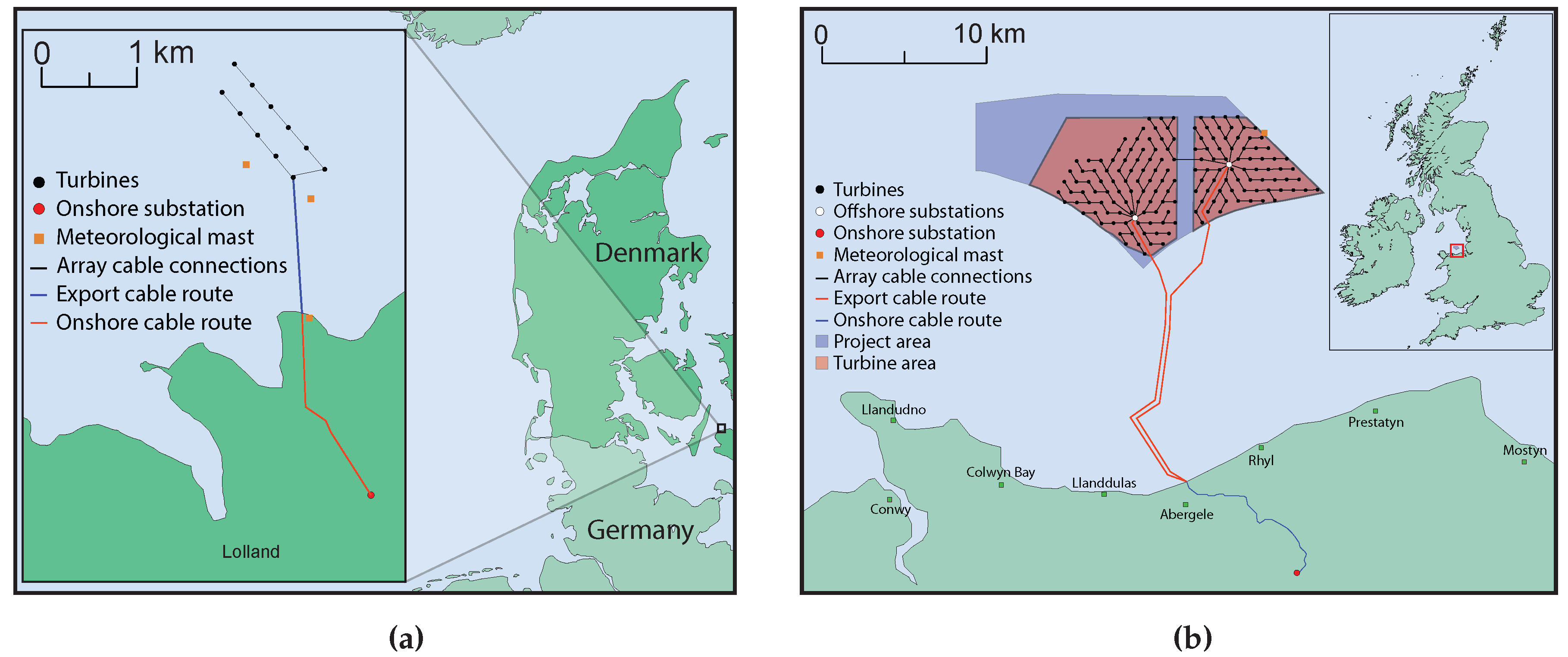
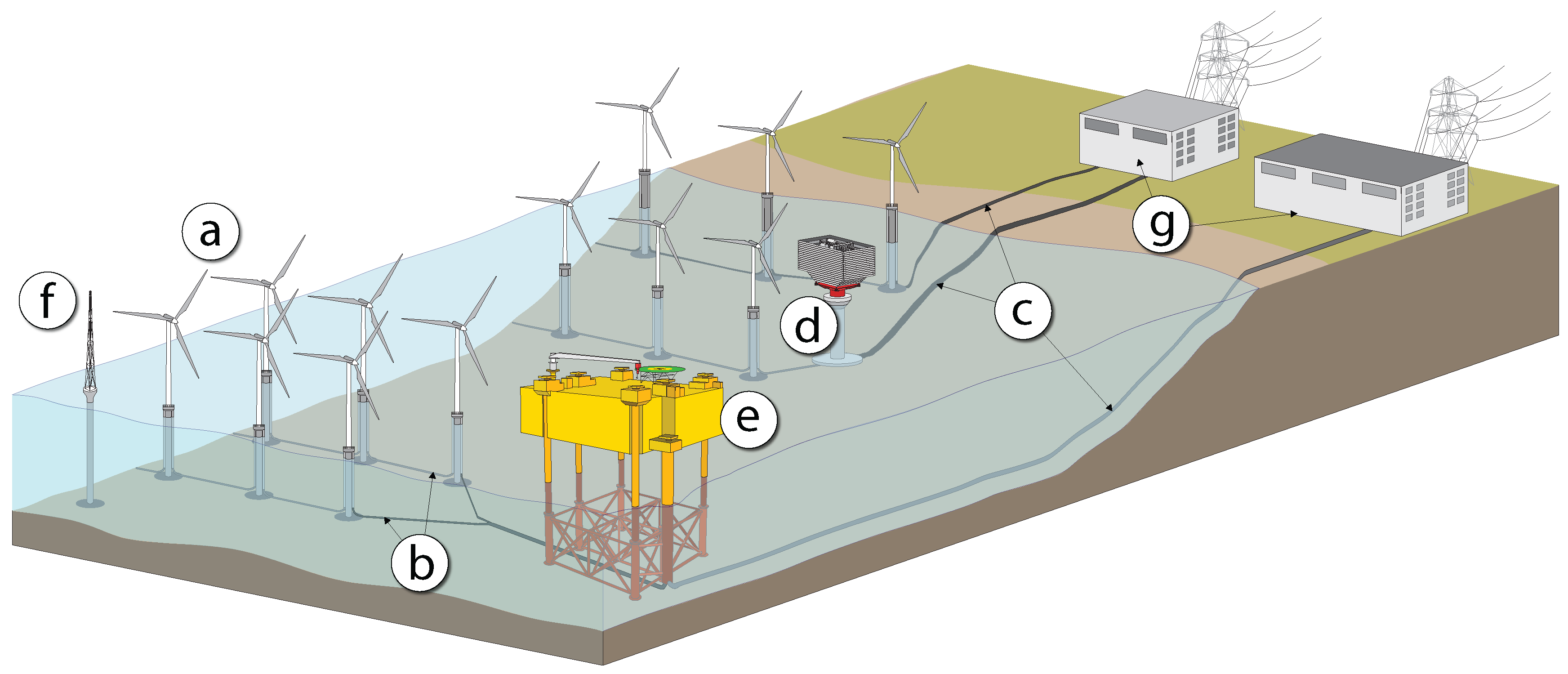
Figure 3 shows the difference in complexity between the first OWF, Vindeby, and the recent British Gwynt y Môr.
Additionally, current design processes are based on a sequential approach (or decoupled strategy) due to the complexity of designing an OWF [19,24]. Such strategy does not guarantee system optimality because the interactions between different system components are disregarded. Moreover, early project decisions may become constraints in later stages [9]. Automated optimization is crucial to optimize the wind farm layout, since the design of OWFs with standard tools is highly complex and time consuming [19]. A reduction of up to 10% in the cost of energy is possible through more integrated design methods [9].
The increased difficulty in the design of modern OWFs comes from the fact that, mostly, all the design aspects of an OWF influence both its energy production and its investment and operational costs [2]. For example, the energy production is increased by placing more turbines in the OWF area, however this also makes the costs rise. Also, interactions between turbines reduce the increase in energy production that results from more turbines being closed together. Hence, these design goals are conflicting, meaning that there is not a single solution for the problem but a set of solutions which represent the trade-off. In the multi-objective (MO) space, a layout is optimal if there is no other layout which is better in all objectives.
Although more than 150 research articles on the wind farm layout optimization problem (WFLOP) may be found in literature, few studies have investigated the inherent trade-offs of designing an OWF [25]. For example, the trade-off between the wind farm capacity factor and the power density within the project area was assessed in [26]. The authors analyzed the conflict between increasing the spacing between the turbines to increase energy production (via a decrease of wake losses) and the need for larger project areas.
Comprehensive studies that explicitly consider multiple goals during the optimization process are rare [27]. Table 1 presents the characteristics of the MO WFLOP (MOWFLOP) from previous studies. The work carried out in [28] optimized the annual energy production (AEP) considering the problem constraints (minimum proximity constraint between wind turbines and area constraint which guarantees that all turbines are placed within the wind farm area) as a second objective function. The AEP and the turbine noise were optimized in [29,30]. Similarly, the AEP was maximized and the sum of the wind farm area and number of turbines were treated as a second objective function in [31]. Three simultaneous optimization goals were used in [32]: AEP, area used and collection system length. The work presented in [33] studied the different features that a MO algorithm should have to efficiently solve the MOWFLOP. The optimization goals were the AEP and the system efficiency, while the optimization variables were the location and number of turbines.
A framework able to efficiently optimize, at once, both the wind farm layout and its respective electrical infrastructure for large OWFs is a highly desired tool by wind farm designers [20,29]. However, none of the optimization frameworks displayed in Table 1 captured all the key aspects pertaining to the development of OWFs. In other words, as far as the authors knowledge a MO optimization framework—which is able to give general recommendations and trade-offs insight to OWF developers—has not yet been established.
To bridge this existing research gap, this article proposes a MO optimization framework to integrate, automate and optimize the design of OWF layouts and their electrical infrastructure. The most suitable and relevant optimization goals and design variables for the MOWFLOP will be identified. The optimization framework is then applied to the design of an OWF in a case study to demonstrate the advantages and differences of the proposed method.
The article is organized as follows: Section 2 provides an overview of the relevant commercial and academic optimization methods for OWFs. Furthermore the most common economic functions used to assess the profitability of wind projects are introduced and explained. Thereafter, Section 3 presents the MO optimization framework for the design of OWF layouts and respective electrical infrastructures and its boundaries and selection criteria. 
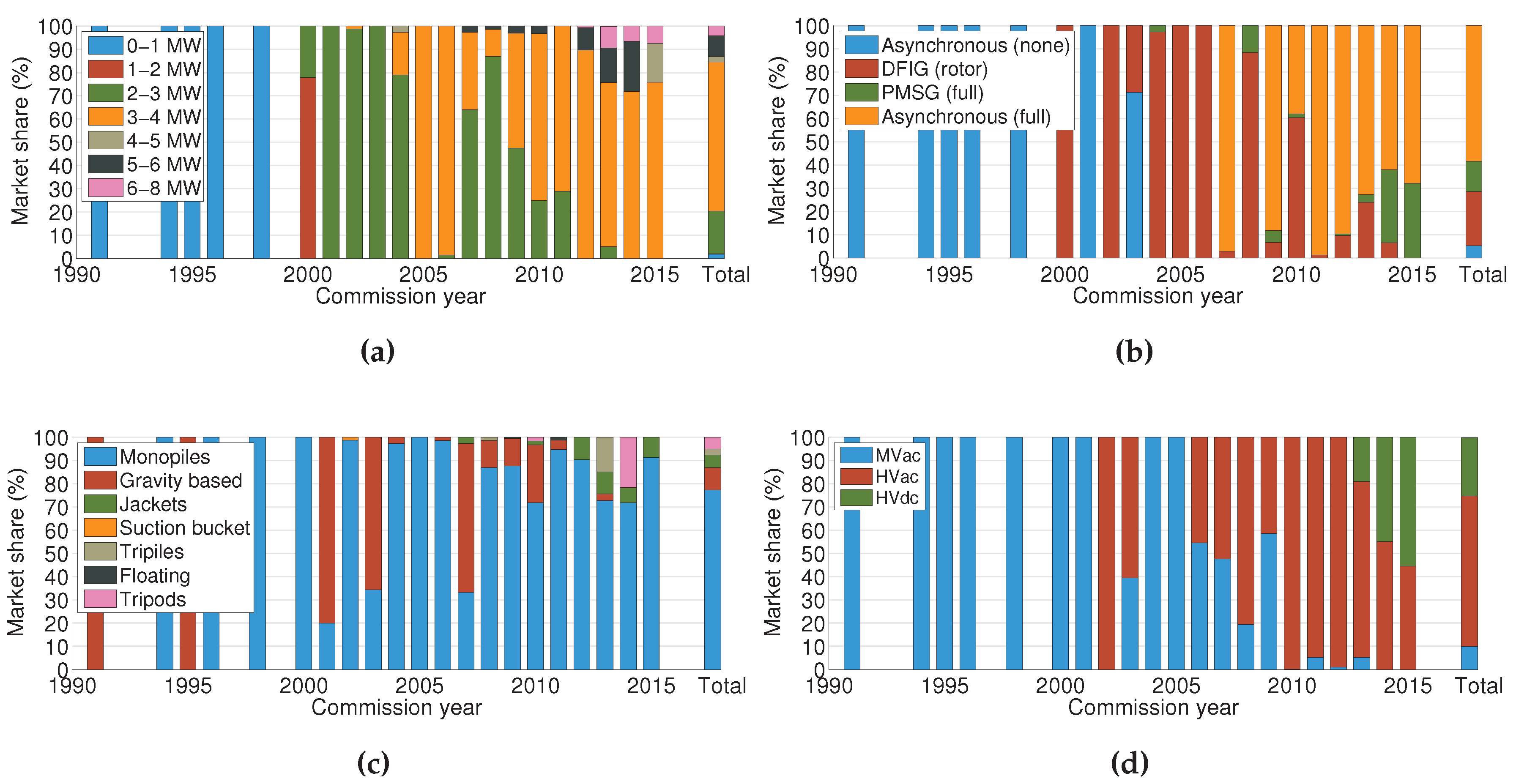
Section 4 introduces the optimization variables considered in the framework as well as their boundaries, constraints and influences over the energy production and expenditures. The industrial trends of the different components of an OWF are also investigated. Section 5 then describes the case study used to demonstrate the usefulness of the proposed framework, followed by Section 6 in which the results obtained are presented and discussed. Section 7 presents the main conclusions of the article.

2. Current Wind Farm Optimization Tools

2.1. Commercially Available Software

Currently, there are several software commercially available to optimize the design of wind farms. For example, WindPRO [36], WindFarmer [37] and WAsP [38] are among the most famous optimization tools. Table 2 presents the main features and limitations of the best-known available commercial software.
All the commercial wind farm design tools were specifically built for onshore environments and, therefore, consider some irrelevant design aspects for offshore areas such as visual impact (irrelevant for far offshore), shadow flickering, noise levels [34] and complex terrain elevations [42,43]. Although it is possible to use them to design OWFs, none of them consider some of the important offshore aspects such as number of turbines, collection and transmission systems design, number and location of offshore substations and transmission technology. Furthermore, no commercial tool uses a MO algorithm to optimize the trade-offs between the chosen goals.

2.2. Academic Studies

On the other hand, several academic studies were specifically tailored to design OWFs. A brief description and the main drawbacks of some of these works are given next.

2.2.1. Offshore Wind Farm Layout Optimization (OWFLO) (2005)

The OWFLO project proposed a framework to design OWFs which uses the levelized cost of energy (LCOE) (€/MWh) as the optimization goal. It includes turbine availability, wake and cable losses and cost models for the turbines, support structures, cables, operation expenditure (OPEX) (bn €), installation and decommissioning [44]. With these models, the OWFLO tool captures the key factors that influence the cost of energy: turbine size, water depth, distance to shore, soil types and wind and wave conditions.
The main goal of the OWFLO project was the development of an optimization software to provide insights into the trade-offs between cost and energy. However, even though both energy and cost models are used, wind farm developers are only presented with one solution at the end of the optimization routine. Hence, no information regarding the existing trade-offs is obtained. Furthermore, the design of the wind farm collection system, which is a key design aspect, was not considered.

2.2.2. Lackner and Elkington (2007)

The trade-offs inherent to OWFs design problems are identified in [45]. These trade-offs are captured by considering the COE as the optimization goal. However, by optimizing directly the COE, the wind farm designers are only presented with one final solution, hence, once again, no information regarding the trade-offs is obtained. Furthermore, the water depth and the wind speed are considered as functions of the distance to shore.

2.2.3. Gribben et al. (2010)

This study presents an OWF layout design tool based on an engineering approach [46]. The authors also identify the multi-disciplinary nature of the problem and, although it is stated that it is important to make a selection of the significant design considerations since it is a highly complex problem, no selection criteria are provided. Moveover, there is no optimization routine implemented in the design approach and only a variation of the design parameters is carried out.
Trade-off insights are presented between, for example, energy yield and foundation costs. Nonetheless, similar to standard design strategies, the method is based on a sequential approach. Moreover, only geometrical layouts are considered and the turbine type is set beforehand.

2.2.4. Topology Optimization of Wind Farms (TopFarm) (2011)

The main goal of this EU-funded project, TopFarm, was the design of an optimization tool for wind farm developers [47]. The financial balance was used as the optimization goal, whereas the turbine coordinates were chosen as design variables. Relevance and relative cost basis were the selection criteria for the cost models in the framework. TopFarm only considered costs which depend on the wind farm topology, since only these provide useful information for the optimization algorithm to guide the search.
Although TopFarm has a comprehensive number of modules, it still lacks key aspects for the optimization of OWF layouts. For example, the collection system routing was determined by solving the auxiliary road problem, i.e., interconnecting all turbines and assuming that the cables could transport all the power connected to them. Furthermore, the TopFarm tool does not consider offshore substations or export cables, which are key factors for OWF developers.

2.3. Economic Functions for Offshore Wind Projects

Investing capital in one project means that the same capital cannot be applied to another investment that is equally or more attractive. Therefore, before final investment decisions are made, wind farm designers create several wind farm designs during the FEED phase to evaluate them economically [2,14].
The choice of which economic function to use is based on different factors, e.g., risk associated, financial structure, regulation, project size [48]. Due to the variety of factors, depending on the case some economic functions are more suitable than others. Therefore, different functions should be used to evaluate possible investments [49]. Table 3 presents the objective functions commonly used in the existing optimization frameworks as well as other economic functions which may be used to assess the profitability of OWFs. Next, a brief description of each function is given and their respective advantages and disadvantage are also discussed.

2.3.1. Annual Energy Delivered

Maximizing the annual energy production (AEP) (GWh/year) is among the most common goals [25] and aims at maximizing the AEP of the wind turbines. Another more comprehensive goal is to maximize the annual energy delivered (AED) (GWh/year) to the onshore electrical network. This goal covers the AEP but also the electrical losses through the entire system, e.g., transformers and cabling systems. Nonetheless, these goals do not take into consideration costs associated with the project or the efficiency of the project.

2.3.2. Utilization Factor

The utilization factor (UF) [–], or capacity factor, of an OWF is the ratio between its AEP and its power production if working constantly at rated power, for the same period of time. This measure is also captured by the wind farm efficiency which is the ratio between the energy delivered over the energy produced without losses. The UF is maximized considering the AED and the efficiency of the system. However, the costs of the project are still neglected if designers use this measure.

2.3.3. Cost of Power

A simple approach to also considerer the CAPEX is to minimize the COP installed which is the ratio between in the CAPEX and the rated capacity of the project. In this way, the optimization tries to maximize the AED and reduce the cost simultaneously. However, and specially in offshore environments, the OPEX also plays an important role in the total costs of the project. Hence, a better approach is to use economic functions which relate the AED, CAPEX and OPEX of the project through economic factors.

2.3.4. Levelized Cost of Energy

The LCOE is also one of the most common economic functions used to evaluate wind farm layouts [25]. The LCOE represents the minimum energy price that meets the desired interest rate by the designers [17]. The LCOE function requires the interest rate and the wind farm lifetime. However, it may not be straightforward to set a value for the interest rate since it is associated with the risk perceived by the investor and it also may change throughout the wind farm lifetime [50]. Furthermore, the LCOE is not suitable to choose between mutually exclusive options for OWF layouts since it does not capture the difference between investment sizes [48].

2.3.5. Net Present Value

The net present value (NPV) (bn €) defines the total profit of the OWF. It considers both the cash outflows (costs) and inflows (revenues) [48]. Therefore, the NPV requires all the economic factors that the LCOE function requires as well as the price of energy. A positive NPV represents a good investment whereas a negative NPV value indicates that the income (with the interest rate chosen by the designers) is lower than the costs [48].
The NPV is suitable to evaluate and compare mutually exclusive projects because it can distinguish the difference in size of different wind farms [48]. Moreover, the NPV should also be used as an alternative measure to further validate the investment [48]. On the other hand, the NPV does not consider, for example, the time required to cover the investment costs (see Section 2.3.7), which may lead the designers to choose a layout that will require a long time to generate profit to the investors.

2.3.6. Internal Rate of Return

The internal rate of return (IRR) (%) is the interest rate that sets the NPV function equal to zero. The IRR function is usually used to approve or disapprove wind farm designs and allows to check if a minimum rate of return set by the designers is met [48]. Nonetheless, the IRR is not suitable to choose between exclusive alternative designs since it does not differentiate wind farm project sizes. Furthermore, the IRR may over predict the profitability of a project because it assumes that the interim revenues are reinvested at a similar rate to the IRR [48]. Finally the IRR does not accurately distinguish the profitability of projects with different lifetimes.

2.3.7. Discounted Payback Time

The discounted payback time (DPT) (years) determines the time, in years, required to cover the initial investment while taking into account the time value of the money. The use of the DPT is recommended when risk is an issue since it represents the period of time in which the capital invested was not recovered, and is therefore, still at risk [48].
The DPT is also not recommended to select one wind farm layout among a set of alternatives because it also does not discern wind farm project sizes. Furthermore, the DPT is not suitable to rank the different possibilities since it ignores the cash revenues after the payback time [48].

2.3.8. Return on Investment

The return on investment (ROI) [–] represents the revenues per unit invested. It is calculated by calculating the ratio between the cash revenue and the initial investment. The ROI is recommended to accepting or rejecting single projects [48]. The ROI is not suitable to choose among mutually exclusive wind farm designs for the same reasons presented before.

2.3.9. Benefit to Cost Ratio

The benefit to cost ratio (BCR) [–] is similar to the NPV function but instead of subtracting the CAPEX to the revenues, it computes a ratio. Higher values for the BCR function represent better wind farm designs. Similarly to other functions the BCR function is recommended to accepting or rejecting single projects but not for selecting among mutually exclusive alternatives. However, it can be used to differentiate the size of the projects if the BCR ratio is obtained with incremental revenues and expenses [48].
To calculate the incremental ratio, the different projects are sorted by increasing CAPEX values and the BCR of the first project is calculated. Next, the incremental differences between the revenues and CAPEX of the second project to the first are obtained. The ratio of these values is then multiplied by the BCR of the first project. If the result is higher than one, the second project becomes the reference. The procedure is repeated until a ratio lower than one is obtained [48].

2.3.10. Annualized Value

The annualized value (AV) (bn €) represents the annual revenues. The AV is constant if no escalation of the price of energy or the OPEX are considered [48].

2.4. Current Optimization Frameworks

Figure 4 shows the current optimization strategy used by wind farm designers. The main disadvantage of this approach is that, by varying the economic factors, e.g., interest rate and price of energy, of the objective functions, it is not guaranteed that the layout solution remains the most advantageous. In fact, optimization strategies that optimize economic functions such as the LCOE or the NPV, may be thought as weighted optimization procedures, in which a MO problem is simplified into a single problem one.
Current single-objective optimization frameworks only output one layout which is, often, pre-constrained due to decision taken before the optimization. An example of this practice is the choice of the wind turbine model or the number of turbines in the initial phase of the design process (see Section 1). However, the designers should not limit the design themselves beforehand but rather should explore all the designs and select the most suitable design only after a careful inspection of economic factors and high-level constraints.

3. Multi-Objective Optimization Framework

3.1. Optimization Goals

All economic functions used to evaluate the profitability of OWFs have the same backbone variables: the AED, CAPEX and OPEX. They were the chosen as optimization goals because they retain their original function direction when optimizing any economic function. In other words, to optimize an economic function f A E D , C A P E X , O P E X , the AED must be maximized and both the CAPEX and OPEX have to be decreased. In this way, it is possible to obtain optimized wind farm designs without setting a priori economic factors, e.g., interest rate or price of energy.
Although MO optimization is generally slower and computationally more demanding than single-objective optimization due to the larger problem search space (optimizing conflicting goals is more challenging than optimizing only one function), the former only requires one optimization routine because it optimizes all the goals simultaneously and therefore the optimization and decision phases are decoupled (see Figure 5). In this way, time is saved since only one optimization routine is run. Afterwards, all the possible results are presented to the designers. Nonetheless, the proposed framework still depends on component costs. The optimization strategy would be more flexible if it differentiated wind farm layouts solely on raw comparisons (e.g., cable length, number of turbines or support structures height) without relying on any costs. However, as for any optimization problem, adding many optimization goals is counter-productive as it raises the problem complexity and largely increases the required computational cost.
The optimization framework targets the FEED phase of an OWF. At this stage the farm layout is not yet decided, but the wind farm location is already defined [15]. Therefore, the macro siting optimization of the wind farm is out of scope. It is considered that the project location resulted from several factors that minimized environmental impacts such as bird and marine life, military activity, nature conservation, shipping and navigation, sub-sea cabling and pipelines, existing offshore industries and aviation [22].
Furthermore, it is assumed that the location has suitable wave and tidal conditions, soil properties, feasible water depths, as well as an economically viable wind resource. Although transportation and installation of wind farm components are not directly considered, part of these costs are captured in the framework by avoiding the most challenging seabed areas and by including an installation cost share in the price of turbines.
Finally, a pre-selection of components, e.g., wind turbines and cables, has been performed beforehand. In this way, the wind farm designers provide a database with information on these components to the optimization phase (see Figure 5).

3.1.1. Selection Criteria

The following criteria were used to select the design aspects to be incorporated in the framework:
  • Topic relevance—only design considerations that are relevant for OWFs should be included. For example, as mentioned in Section 2, visual impact, shadow flickering and noise are not relevant in offshore environments [15,19,51] although they are highly relevant when designing onshore wind farms.
  • Impact—the optimization framework should include design features that play an important role in the wind farm layout. This is because the optimization algorithm needs to capture the difference between the wind farm layouts [47].
The trends of the different components will be assessed in the next section to assure that the components selected in the case study of the paper are representative of the current offshore wind industry. Furthermore the trends of the components will also identify the important design characteristics, e.g., number, location and type of offshore substations, that need to be implemented in the optimization framework.

4. Selected Design Aspects and Optimization Variables

This section presents the optimization variables and respective design aspects which, based on the aforementioned selection criteria, should be considered in the optimization of OWF layouts and their electrical infrastructure. The optimization variables and design aspects are presented separately for the main components of an OWF: turbines, offshore substations and cables (shown in Figure 6). Table 4 summarizes all the design aspects with their respective boundaries and constraints. Furthermore, it also shows the direct influences of the design variables over the AED and CAPEX. Next, the industrial trends of each optimization variable are given to assure that the optimization framework here presented embraces all the important points of current state-of-the-art OWFs.

4.1. Wind Turbines

Figure 7 shows that the rated power, rotor diameter and hub height of offshore wind turbines is increasing since the initial projects. The average turbine rated power installed between 2012–2014 rounded the 4 MW mark (see Figure 8a) [53]. This means that, generally, the offshore wind industry prefers larger wind turbines.
The electrical systems of wind turbines have also evolved. Figure 8b shows that the first turbines used simple fixed-speed systems with asynchronous generators and with no power converters [55]. In a second technological step, pitch-controlled variable speed wind turbines technologies emerged as the preferred technologies and became the dominating type of wind turbines in the following years. Wind turbines equipped with doubly-fed induction generators (DFIGs) constitute approximately 25% of the offshore market [10]. Nowadays, most of the offshore wind turbines are equipped with fully-rated voltage source converters (VSCs) in a back-to-back configuration. These converters allow for enhanced controllability which helps to meet the challenging grid code requirements and the reduction in mechanical loads achieved with variable-speed operation [56].
Regarding the support structures, Figure 8c shows that the monopiles have the highest market share, although different grounded support designs, e.g., tripods, gravity based and jackets, have been tested. Figure 9 shows the most common support structures and two innovative designs: the suction bucket and the twisted jacket [57,58]. Nonetheless, monopiles are expected to maintain their market share for the coming years since efforts are being done to enhance the design of monopiles to be able to support 6–8 MW turbines in water depths up to 40 m [59].
In the far future, floating support structures are expected to obtain a fair share of the offshore wind market due to their use in deep waters [60]. Figure 9 shows several floating solutions which have been tested in the last years. However, much has to be done before floating solutions become economically more viable than monopiles [60].

4.1.1. Design Variables, Constraints and Influences

The number, model and location of the turbines have to be simultaneously optimized to guarantee that enhanced layouts are obtained. The locations of the wind turbines have a strong impact on the overall efficiency of the wind farm. The turbines energy production is directly related to the turbines power curve and to the wind resource specific from the wind farm area. Installing wind turbines close to each other causes interferences such as shadowing effects, which lead to reduced power production and, therefore, lower wind farm efficiencies. For example, the Danish Horns Rev OWF produces 11% less due to wake effects [65].
Different turbine models have distinct market prices, hence, it is important to evaluate the influence of the number of turbines and respective types in the CAPEX. Also the support structures have to be assessed since the turbine model and water depth and soil properties play a major role. Support structure costs are typically dominated by the steel price and the influence of the water depth and ground conditions on the structure design [13]. In fact, the support structures investment cost does not scale linearly with their height. Therefore, costly support structures may be prevented if deep locations of the wind farm area are avoided. The proposed optimization framework needs to address the dependency of the cost of the turbine support structures with the seabed water depth.

4.2. Offshore Substations

Since 2002 most of the OWFs make use of offshore substations to increase the voltage levels of the transmission system (see Figure 8d). Currently, there are two types of offshore substations: transformer substations, that simply increase the ac voltage to suitable transmission levels; and converter substations which also perform ac to dc conversion (and viceversa).

4.2.1. Design Variables, Constraints and Influences

The number and location of substations is an important design aspect as it directly impacts the total length of the collection system [66]. The number of substations has also a strong impact in the wind project CAPEX, as well as type of substation. Converter substations are much more expensive due to their larger size and weight, but also due to the extra components required to rectify ac into dc. Furthermore, the type of substation also defines the transmission technology, which plays an important role in the overall system cost and electrical losses [67].
Figure 10a shows that initially one external substation was commonly used, i.e., the substation was placed at the edge of the projects. In a second step, the substation started to be inside the wind farm to minimize the collection system length. Nowadays, large OWFs usually make use of two offshore substations as shown in Figure 3b [10,11]. In this way, an optimization framework has to be able to place offshore substations both inside and outside the wind turbines as well as handle multiple offshore substations.

4.3. Collection Cables

The collection cables interconnect different wind turbines and transport the energy generated to an offshore substation or to shore if no substation is present. More precisely, the collection cables connect to the switchgear inside the turbines to the switchgears of the substation [19,68].

4.3.1. Design Variables, Constraints and Influences

The main design variables of the collection cables are the rated voltage and their cross section which is related to their rated power. So far, 33 kV is the highest and most common voltage level in wind farm collection systems [10]. If a 66 kV collection system was used, the transmittable power would double but the costs would increase by 12% [69]. Therefore, the voltage level of the collection system has to be assessed to assure that optimized layouts are obtained.
The cable layout design is performed during FEED studies and several topologies may be used, e.g., radial, looped or branched arrays [15,70,71,72,73]. The design of the collection system plays an important role in the electrical losses. For example, the use of branching may lead to shorter collection systems (Figure 3b shows an example of a branched collection system) and, hence, lower installation costs [74].
The usage of cables with different cross sections is another strategy to reduce the investment costs related to the cabling system. Figure 10b shows that, hitherto, the offshore industry has opted to use array cables with different cross sections only if the total array cable length was above 25 km (an exception is the British Greater Gabbard wind farm) [52]. This strategy allows for costs reduction because cables that carry the power of only a few turbines have lower cross sections and, therefore, need less raw material [75].

4.4. Transmission Cables

Initial OWFs exported their energy production via medium-voltage ac (MVac) transmission systems since the transmission losses were low due to their low installed capacities (up to 100 MW) and close proximity to shore (shorter than 15 km) [22]. The need for an offshore transformer came from the high installed capacities and higher distances to shore [22]. In 2002, the Danish Horns Rev 1 became the first project to make use of an offshore transformer station [10].
Thus far, the industry has used the high-voltage dc (HVdc) technology when distances higher than 50 km and installed capacities above 100 MW were considered [22].
Although HVac technology is used to transport 65% of the energy generated offshore and the HVdc technology accounts for 25% of the total installed capacity (see Figure 8d), currently it is still unclear if one technology will obtain a large share of the market or if several technologies will be used [22]. Therefore, it is desired to obtain an optimization framework that accounts for the different transmission technologies.

4.4.1. Design Variables, Constraints and Influences

The type of cable has a direct impact in the overall system cost as well as in the transmission losses. Furthermore also the cross section of the cables is directly linked with their power transfer capability. Finally, the rated voltage of the transmission system also relates with the power losses and with the obtainable transmission distances. This is of high importance when HVac systems are considered due to the large reactive power compensation needs [76,77,78].

5. Case Study

The key variables during the design of an OWF, the optimization goals and the need for MO optimization were introduced in the previous sections. Now, the proposed framework is applied to a case study to demonstrate the advantages and the design capabilities given to the designers.

5.1. Borssele Wind Farm

In 2013, the Netherlands defined an Energy Agreement which set as target to increase its renewable energy production by 14% until 2020 [79]. To achieve this target the government has allocated up to € 18 billion to subsidize the offshore wind industry. The Energy Agreement identified the need for an additional offshore capacity of 3.5 GW by 2023. For this purpose, 700 MW licences and respective subsidies will be tendered annually between 2015 and 2019 [80].
Several areas, shown in Figure 11, have been identified for the development of OWFs. The areas Borssele, IJmuiden Ver, Hollandse kust and Ten Noorden van de Waddeneilanden cover approximately 2900 km2 (representing 5% of the Dutch EZZ [81]) and have a potential offshore wind capacity of 17.4 GW (assuming an average of 6 MW/km2) [82].
The first two zones of the Borssele wind farm area are considered for the case study. The Dutch Borssele wind farm zone is situated 0.5 km away from the Belgian exclusive economic zone [83] and has a total area of 344 km2 which is divided into four sites with a maximum installed power of 350 MW each (see Figure 12a) [83].
Two 700 MW platforms will be built in the Borssele area [80]. Each platform will connect two sites to the onshore grid via 220 kV ac cables [83,84]. The developers have a maximum bid value of 0.124 €/kWh for the Borssele zones I and II [83]. The collection system is planned to have a rated voltage of 66 kV [83,85].
The wind farm area, mean water depth and existing pipelines or telecom cables are shown in Figure 12a. The water depth ranges between approximately 16 and 38 m [83]. The presence of unexploded ordnances (UXOs), which are likely to be present at the site, are neglected since they will be removed if necessary by governmental agencies without additional costs to the wind farm developers [87,88].
Although, most of the existing wind farm projects make use of a standard grid layout [10,11], this is not the case for the Borssele wind farm area in which there are no restrictions regarding the placing of the turbines [89,90].
The wind resource data (see Figure 12b) was measured at four different locations [91]. The measurement points are located between 15 to 82 km of the offshore wind farm and the measurement height varied between 21 and 315 m above sea level [91]. The measurement campaigns were carried between 5.5 months to 12 years [91]. The long-term mean wind speed at a hub height of 100 m above sea level at the center of the Borssele zone is 9.6 m / s [91]. The wind speeds were extrapolated to the turbine hub heights to account for its vertical profile [92]. The mean wind speed at hub height of the Vestas turbine (107 m) is 9.67 m / s , whereas for the Darwind turbine (hub height of 92.5 m) a value of 9.52 m / s is obtained. Lastly, it was considered that the wind turbines could operate during 80% of the time for wind speeds higher than 18 m/s, i.e., during 80% of that time the wind speeds were lower than 25 m/s and, in this way, the turbines operate. For wind speeds higher than 25 m/s the turbines have to be shut down for safety reasons (see Figure 13).
Lastly, the point of common coupling (PCC), situated in Borssele, is approximately 50 km away from the wind farm area [93] and the length of the export cables are considered to be 15% longer than the distance to shore to account for any necessary rerouting of the transmission cables (see Figure 3b).

5.1.1. Component Data

Turbines

The turbines considered in the case study are the Vestas 8 MW with a rotor diameter (RD) of 164 m and hub height of 107 m [94] and the Darwind 5 MW with a 115 m rotor diameter and a hub height of 92.5 m [95]. Figure 13 presents the power and thrust curves of both turbines. Since these curves represent the power delivered at the output of the turbine, it is not necessary to calculate the power losses in the turbine electrical system [25]. Both turbines makes use of full-rated power converters connected in back to back. A minimum separation between two wind turbines has to be respected [96]. In this case study a minimum distance of 4RD was used [84].

Cables

All cables are modeled with a π-model which takes into consideration the type of soil surrounding the cables and the geometric dimensions of the cable according to the IEC standards 60228 and 60287 [97,98]. For a thorough description of the cable model the reader is referred to [76,99]. Table 5 presents the properties of the all the cables used in the case study. The 33 kV cables (240 or 500 mm2 of cross section) are able to carry 5 or 8 Darwind turbines; and 3 or 5 Vestas turbines, respectively. Regarding the 66 kV cables, they could carry the power of 11 or 16 Darwind turbines; and 6 or 10 Vestas turbines, respectively.

Multi-Level Modular Converters (MMCs)

A MMC steady-state model recently introduced in the literature is used in this work [76,101,102]. The model captures the conduction and switching losses of the semiconductors, the conduction losses of the arm reactors, the cooling system losses and the influence of the temperature of operation. The MMC is based on Infineon IGBTs and its properties are shown in Table 6 [103]. The MMC is considered to balance the voltage of the capacitors of the submodules through the reduced switching control strategy which lowers the switching losses and allows the efficiency of the MMC to be close to 99.5% [101].

Transformers

The transformers are modeled with a T-model which considers the core and ohmic losses (see Figure 14) [76,99]. The transformer parameters (shown in Figure 14) are based on the three-phase transformer of the SimPowerSystems toolbox of MATLAB Simulink [76].

5.2. Optimization Goals

5.2.1. AED

Energy Production

The energy generated by the turbines is calculated based on their power curves. The availability of the turbines is considered to be 97% which is a value envisioned to be obtained between 2015 and 2035 [104].

Wake Losses

The Jensen model was used to calculate the wake interaction between turbines. The Jensen model, one of the most common models used, is a simplified and fast manner of calculating the wind speed inside the wake of a turbine [25]. More precisely it was used a later version of the model, which was developed by Katic et al. [105]. All the MO approaches presented in Table 1 used the Katic-Jensen model (except [29,30] which used the original Jensen model). For a description of the wake model the reader is referred to [105,106,107].

Collection System Design

Finding the optimal branched infield cable topology for OWFs corresponds to the capacitated minimum spanning tree problem [108]. A savings heuristic approach is used since the optimization framework requires fast models. It is a hybrid between the heuristics Planar Open Savings [72] and Esau and Williams are the possibility for multiple cable capacities, the minimization of pipeline/cable crossings and the option to select the maximum number of cables branches per turbine [75].
It is assumed that the collection system connects every turbine to one substation through one distinct cable. The inter-array cables cannot cross each other or the transmission lines of their substation. The maximum number of cable connections per turbine is considered to be four due to space limitations inside the turbine tower [68,85]. Finally, the crossings with existing pipelines and telecom cables should be minimized [66,109]. For a more detailed explanation of the heuristic the reader is referred to [75].

Electric Infrastructures

Three different transmission technologies (TT) are considered in this work: MVac, HVac and HVdc (see Figure 15). The MVac interconnects directly the turbines to the PCC, whereas the other two options make use of offshore substations.
Recent studies investigated the advantages of using an overplanting strategy. Such design strategy breaks the common rule used up to now of using a transmission system with the same power capacity of the wind farm. The main idea is to harvest energy from more turbines for low wind speeds and apply curtailment strategies when the wind speed is too high [110].
This idea is implemented in the HVdc scenario by setting the MMC rated power as the sum of the turbines rated power that are interconnected to it. Since the number of cables per MMC is fixed, it is assumed that if the chosen cables have not enough energy transport capacity, the algorithm upgrades them to have larger cross sections. If the cable with the highest cross section available is not able to carry all the power, the MMC caps the power that flows through it to its rated power and the rest is curtailed.
For the case of HVac technology if there is at least one power flow in which the chosen cable is not able to transport all the power, the number of cables of that substation is increased by one and the power flows are run once again. Lastly, the number of turbines that could be connected to each MVac cable is calculated assuming the turbines to operate with a power factor of 0.95 to allow for some reactive power transport [85].

Power Flows

The power flows from the turbines to the PCC are calculated using a power flow and optimal power flow solver library developed in the Python programming language called PyPower [111]. There are three possible types of nodes in a network: PQ, PV and slack nodes. A node PQ is a node in which the active and reactive power are known and the state variables are defined as the load angle (δ) and voltage. On a PV node the active power and voltage level are known but the reactive power and δ are unknown [77]. Finally, on slack nodes a reference angle and the voltage are set but the active and reactive powers are not determined before solving the load flow. Table 7 shows a comparison between the different types of network nodes.
The turbines are considered to be nodes of type PQ, i.e., the active power is set to the values obtained with the wake losses model and it is considered that the turbines are not producing any reactive power. In this way the power flow equations determine the voltage and angle at the turbine nodes. Alternatively, the turbines could be set as PV nodes to help in the reactive power support. However, this falls under the wind farm power control which is out of the scope of this work.
The ac side of the MMCs and the onshore network nodes are defined as slack buses, i.e., the voltage is equal to 1 pu and the angle δ is set to zero degrees. The transformer nodes are considered to be of type PQ and with no net injection of active or reactive power flowing into their nodes. The sizing of the transformers is initially done by summing the turbines rated power which are connected to it. After running the power flows if the rated power of the transformers is surpassed, these become the new values and the power flow scenarios are repeated.
The reactors nodes (see Figure 15) are considered to be of type PV (see Table 7). It is considered that no active power flows to the reactors and that the voltage is equal to 1 pu. In this way, the reactors provide total reactive power compensation. The reactor sizing is based on the scenario in which no power is produced at the turbines, since it represents the most demanding case for the reactive power compensation units [77].

5.2.2. CAPEX

The cost models used in this case study are based on several literature works [49,74,85,112,113,114,115] and it is not the scope of this work to further develop or validate them. The cost values used are updated considering an annual Eurozone inflation of 1.85% [12].

Turbines

The price for the turbines is obtained using the data in [74]. The cost of the Darwind turbine is 4.85 M€ and the Vestas 8 MW costs 6.39 M€. The values include 10% extra for the transport and installation.
If the 66 kV collection system is used, the cost of the turbines increases by 20% due to the extra costs of the turbine transformers and switchgears [85].
The cost to decommissioning the turbines at the end of the wind farm lifetime is set to 1.05 M€ for the Darwind turbine and 1.68 M€ for the Vestas 8 MW [116].

Support Structures

The cost of the monopile support structures and their transport and installation is given by [74]:
C s s = 0.54 · P rated t u r b 1 + 0.02 w d 8 1 + 0.8 · 10 6 h R D 2 2 10 5
where C s s is the support structure cost in M€, w d is the water depth in meters, h is the turbine hub height in meters, R D is the rotor diameter in meters and P rated t u r b is the turbine rated power in MW.

Cables

The cost values of the 33 kV collection cables are obtained from [74] and are shown in Table 5. The cost of the 66 kV cables is considered to be 15% more expensive than the 33 kV cables for similar cross sections [85]. The cost to install the MVac cables is considered to be 365 k€/km independently of the voltage level or the cable cross section [74,85].
The costs of the HVac cables are based on values taken from [114] and are shown in Table 5. An additional cost of 720 k€/km is added to account for the installation of the cable [74]. The costs of the HVdc cables are based on [115] and are also shown in Table 5. Similarly to the HVac cables, the installation had an extra cost of 720 k€/km [74].
The cost to cross an existing pipeline or telecom cable is considered to be 100 k€ [75].

Switchgears

The switchgears for the 33 kV collection system cost 73.25 k€ and the 66 kV ones cost 101.25 k€ [114]. One MV switchgear is installed in each collection cable as shown in Figure 15. The HV switchgears cost 1.57 M€ for a rated voltage of 132 kV and 2.60 M€ for 220 kV transmission systems [115].

Offshore Substations

The cost of the HVac offshore substations is given by [114]:
C s s H V a c = 2.8286 M + 0.099 P s s
where P s s is the sum of the substation turbines rated powers (in MW) and C s s H V a c is the cost M€.
The same expression is used for the HVdc substations but with an 85% increase to account for the larger and heavier structure needed to house the extra components [117].
The cost of reserve diesel generators to run the essential equipment of the substation is given by [74]:
C g e n = 0.0237 M + 0.0023 P s s
where P s s is the sum of the rated powers of the turbines that interconnect to the substation (in MW) and C g e n is the cost of the diesel generator in M€.

Transformers

The transformer costs are expressed as [74]:
C t r a f o = 0.0477 P t r a f o 0.7513
where P t r a f o is the rated power of the transformer in MVA and C t r a f o is the cost in M€. The minimum transformer rated capacity is considered to be 50 MW.

MMCs

The cost of the MMCs is given by the following expression [115]:
C M M C = 61.3777 M + 0.0657 P M M C
where P M M C is the rated power of the MMC in MVA and C M M C is the cost of the MMC in M€. The minimum MMC rated capacity is consider to be 500 MVA.

Reactive Power Compensation

The 33 kV reactors are considered to have an efficiency of 98% [118] and cost 66% of what a transformer of the same rating would cost [114]. A 40% extra cost is added to the 66 kV reactors due to their higher volume and weight [85].

SCADA, Project Development, Insurance

The SCADA system is considered to cost 0.75 M€/turbine [74], whereas the project development is estimated as 0.468 M€/MW [74]. The insurance and contingencies during the project phase are considered to be 0.7 M€ per Darwind turbine and 1.12 M€ for the Vestas turbines [116].

5.2.3. OPEX

The operational costs are an important component of OWFs and, hence, should be considered during the optimization phase. Inasmuch to use a more comprehensive OPEX calculation model, such as the OPEX Cost Estimator from ECN [119], a considerable amount of data is required, e.g., available vessels, crew members and detailed weather information.
Simpler approaches can be used to avoid this drawback. The OPEX may be considered as a percentage of the investment costs [44,45] or monetized through a cost value per MWh produced by the farm [49,120,121]. Because the value of the OPEX is directly proportional to either the AED or the CAPEX, it is not included in the optimization process and is only calculated afterwards. In this way, the problem becomes bi-objective with the AED and CAPEX as optimization goals.

5.3. Multi-Objective Gene-Pool Optimal Mixing Evolutionary Algorithm (MOGOMEA)

The Multi-objective Gene-pool Optimal Mixing Evolutionary Algorithm (MOGOMEA) was used in this work. The MOGOMEA, recently introduced in the literature [122], is a metaheuristic discrete MO optimization algorithm which demonstrated to outperform, i.e., obtain better optimized trade-offs, other state-of-the-art well-known MO optimization algorithms on standard combinatorial benchmark functions [122], as well as in real-world applications [33,123] for a given budget of function evaluations. Although the MOGOMEA is capable of obtaining high-quality results, it does not guarantee global optimal solutions are found given a finite amount of evaluations of the optimization functions [122].
Since the MOGOMEA only uses discrete variables, it is straightforward to optimize the number and locations of turbines in simultaneous. Constraints on the location of turbines, such as minimum distance to existing power cables and shipwrecks, within the OWF area are automatically respected by not considering constrained places in the possible set of locations for the turbines [47]. Furthermore, the limited precision offered by the models used, such as the wake model, do not require the accuracy of continuous variables [33]. The location of a turbine may be described by a single parameter in a discrete approach, whereas a continuous domain demands two variables. Lastly, given the same number of problem variables and the same inherent underlying problem complexity, continuous optimization problems are typically slower to solve than discrete problems because of the larger variable-domain size of continuous variables [33].
MOGOMEA is started by initializing n solutions (the definition of a solution is later introduced in Equation (6)) which are evaluated to obtain their objective values. The algorithm then alters solutions into offspring by exchanging variables between different solutions. The MOGOMEA clusters solutions that are in the same objective space vicinity and only performs variation within each cluster since solutions tend to be very dissimilar for different areas of the objective space [122].
The general variant of the algorithm uses the mutual information as measure to build a hierarchical linkage model to identify group of variables that are important to be copied together under black-box optimization, i.e., nothing is known about the optimization problems [124,125]. However, it is known that turbines influence the energy production of neighboring turbines and that this influence might be considered negligible for turbines situated far enough apart [126,127]. For this reason, in this work the distance between the possible locations is used as a measure of dependency instead of the standard statistical analysis used in MOGOMEA [33].
The population size used by the algorithm is an important internal parameter that should be adjusted according to the instance of the WFLOP being solved [127,128]. A population-free sizing scheme of MOGOMEA is used, avoiding the need for the right population size to be assessed [33]. In this way, the population size is incrementally increased throughout the optimization [33]. This is done to allow new genetic material into the population since the algorithm performs a very intensive local-search strategy and hence, it may fail to layouts that cannot be reached from the initial solutions (only through mutation) [122].
Although the MOGOMEA was initially designed to have a population of solutions that are sequentially altered to generate offsprings [122], the version of MOGOMEA employed evaluates the solutions in an asynchronous parallel manner. Currently, it is becoming even more important to move towards a parallel environment in which several CPU cores may be used simultaneously [129]. This is of high importance especially because the evaluation time of a solution varies with the complexity of the OWF layout it represents. For example, the wake loss evaluation highly depends on the number of turbines [126,127] and wind directions [107], whereas the collection system design also depends on the number of turbines of the project [72,75].

5.3.1. Optimization Variables

A solution is composed as follows:
x = t 1 t i V H V a c C H V a c V H V d c C H V d c V M V a c
where t 1 t i determine what is placed in each available position of the wind farm area. The following representation is used: 0—Empty, 1—Darwind 5 MW turbine, 2—Vestas 8 MW, 3—Transformer substation, 4—Converter substation. The variables V H V a c , V H V d c and V M V a c determine the voltage level of the HVac, HVdc and MVac cables, respectively. The variables C H V a c and C H V d c identify the cross section of the cables.

5.3.2. Random Wind Farm Layouts

An heuristic that aims at maximizing the distance between turbines is used to create random layouts. Firstly, the number of turbines of the wind farm, m, is randomly generated between one and the number of locations of the grid. The location of the initial turbine is randomly chosen from all the possible locations. After, the distances of the remaining possible locations are computed to the first turbine and the most distant location is chosen for the second turbine. The distances f the remaining locations are updated by checking whether the distance to the new turbine is smaller than the currently stored distance (the shorter distance is kept). The procedure is repeated m times or until a turbine violates the proximity constraint. In this way, it is guaranteed that feasible wind farm layouts are generated, similarly to previous works [130,131,132].
Whenever a turbine is placed in the layout, the algorithm randomly selects a turbine model from the ones considered. At the end, the turbine model used in the OWF is the one that was assigned the most since, generally speaking, OWFs are composed of only one turbine type [10,11]. Nonetheless, the framework was designed as is so that this constraint could be removed in the future, if desired.
A random number of substations is sampled between zero and three. Next, the k-means clustering algorithm is run with that same number [133]. The closest locations of the grid to the cluster centroids are chosen to represent the substations. Thereafter, another random number is sampled for each substation to decide if it represents either a converter or a transformer substation. In case there is at least one converter station, the algorithm considers that all substations perform ac-dc conversion, i.e., the transmission system uses the HVdc technology.

5.3.3. Multi-Resolution

The results obtained in [33] indicate that it could be beneficial to use a multi-resolution scheme in which a large grid step is employed in the first optimization iteration to allow the algorithm to find highly packed wind farms easier. Thereafter, these solutions would serve as initial population for a second optimization routine with a smaller grid step. Therefore, the algorithm starts the optimization routine with the 4RD grid step and advances to smaller step sizes of 2RD and 1RD. The layouts are then mapped onto the finer grid.

5.3.4. Internal Parameters

The initial population size, n, is set to 32 since it corresponds to the number of CPU cores available. The algorithm groups the wind farm layouts into five clusters during the optimization process since this setting has proved to already provide improved results over using a single cluster in recent literature [122].

6. Results

The case study was run in Python on a server with 32 cores (Intel Xeon [email protected] GHz) running the 64-bit version of Ubuntu 12.04. The optimization framework was given in total 30 days to run. The largest grid step (4RD) size was run for 6 days, whereas 12 days were given to each of the two remaining more refined grid steps (2RD and 1RD).

6.1. Optimized Trade-off

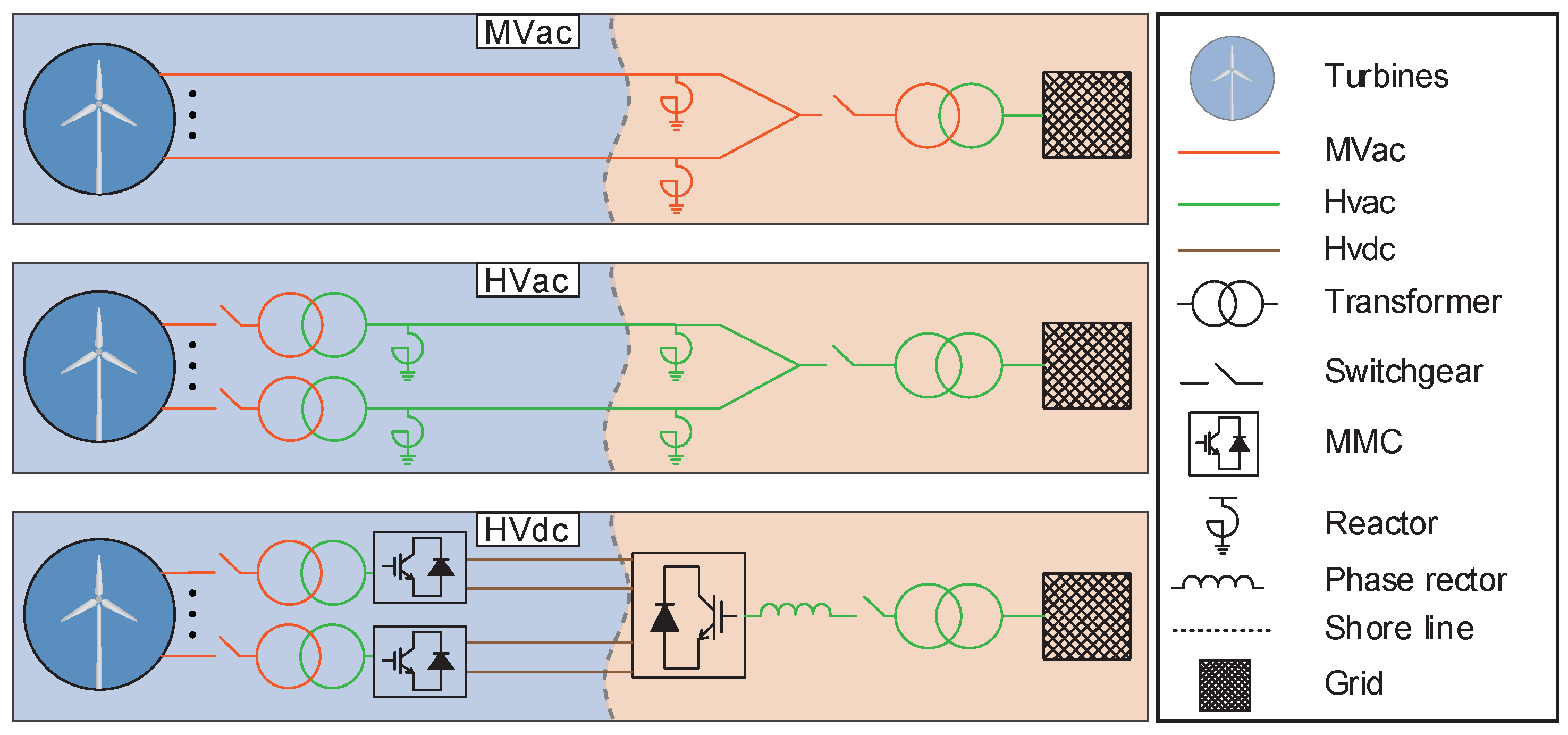
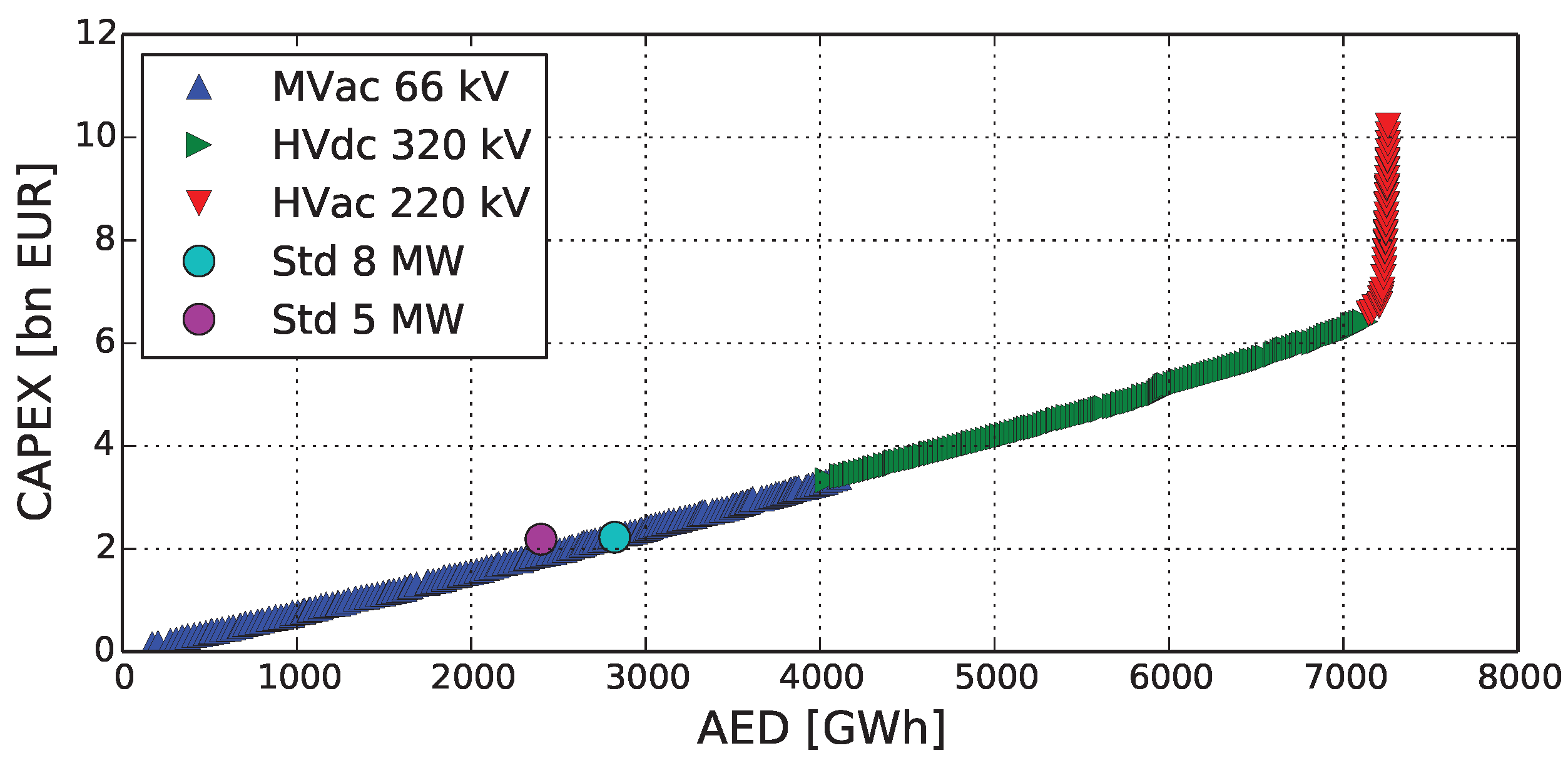
Figure 16 shows the optimized trade-off obtained with the MO optimization algorithm (and for the two layouts designed by hand, which are introduced next) between the AED and CAPEX. The trade-off, composed of 358 different OWF layouts, shows that three different transmission technologies were used. For small wind farms the 66 kV interconnection to shore was the best option. On the other hand, for AEDs higher than 4000 GWh/year, the HVdc transmission technology was used. In the right-hand extreme part of the trade-off curve the HVac technology was used. However, it came with much higher investment costs and did not increase the AED significantly.
Although the optimized trade-off shows a linear relationship between the goals up to an AED of approximately 7000 GWh/year, it is important to note that nothing guarantees that the layouts that are in a close vicinity in the objective space, are also similar in variables space, i.e., the layouts and technologies may vary considerably.
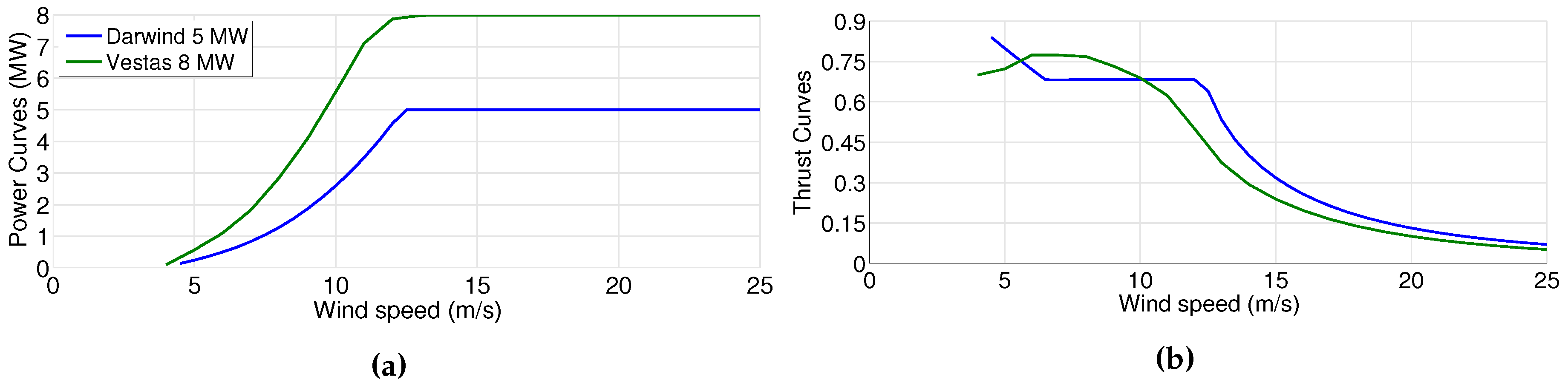
The optimization case study had also the possibility to use the Darwind 5 MW wind turbine; however, no layout that is present in the trade-off used it. The results for the standard layouts also corroborate this result: although the wind farm layout composed of Vestas 8 MW turbines is situated in the trade-off, the OWF with Darwind 5 MW turbines performs much worse than the other layouts. The Darwind 5 MW wind turbines produced less energy and, even though they are cheaper, this difference did not suffice for profitability.
The data gathered for this specific case study hinted that the best turbine was the Vestas one. However, this result is specific for the case study of this paper and should not be generalized since turbines with lower rated powers could be the best option under different circumstances. For example, the support structure costs, insurance costs, among others, do weight in the decision making. Although, one turbine demonstrated to be clearly superior for this case, for other scenarios, e.g., different wind farm area or distance to shore, the outcome could differ.
A more difficult situation would be when one could not have a direct hint from the specifications of the wind turbines. Under such scenario, the advantages of the proposed optimization framework would clearly stand out. Furthermore, the optimization framework is also able to select from several wind turbine types (more than two), which is a very difficult selection process to be manually performed.

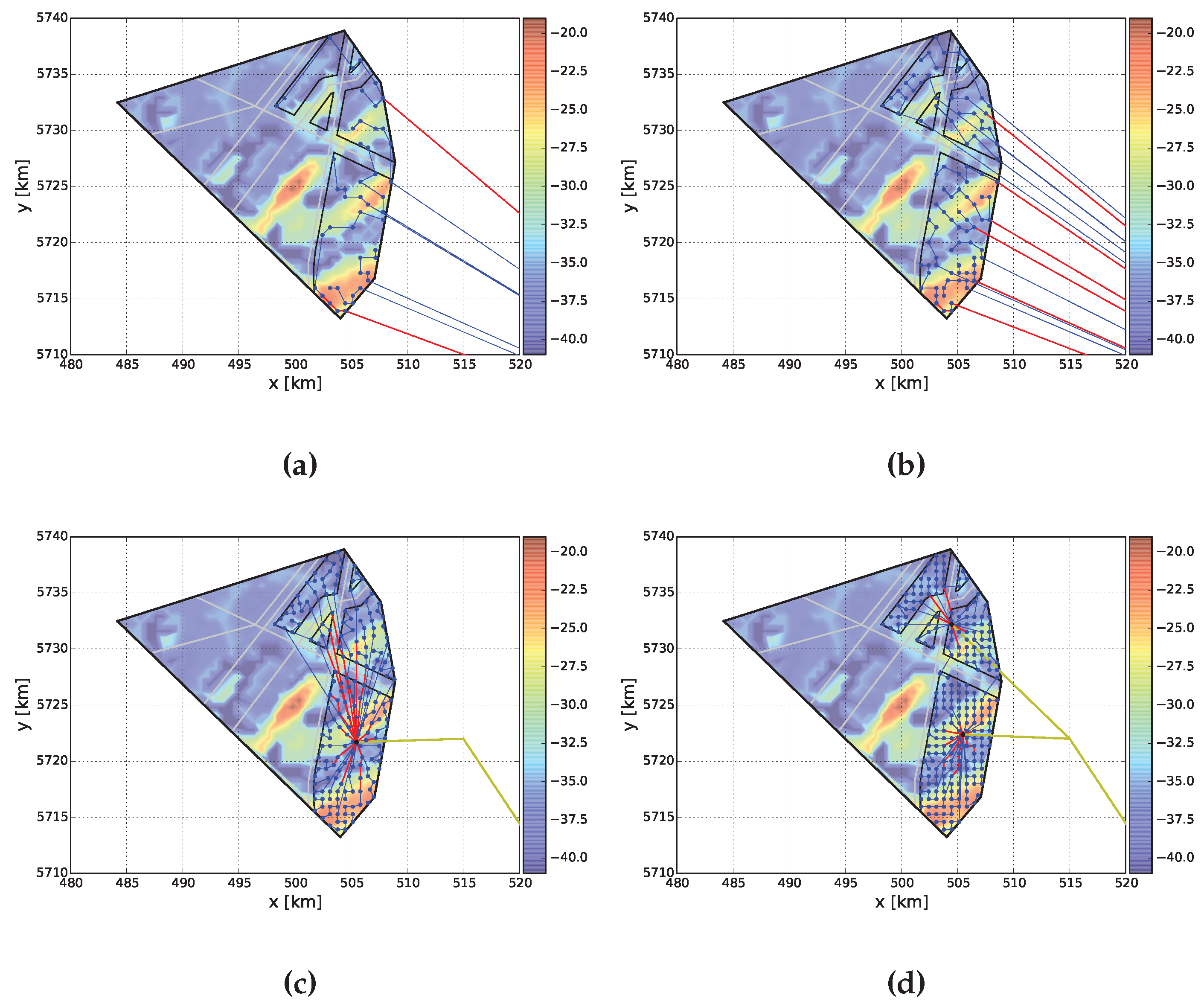
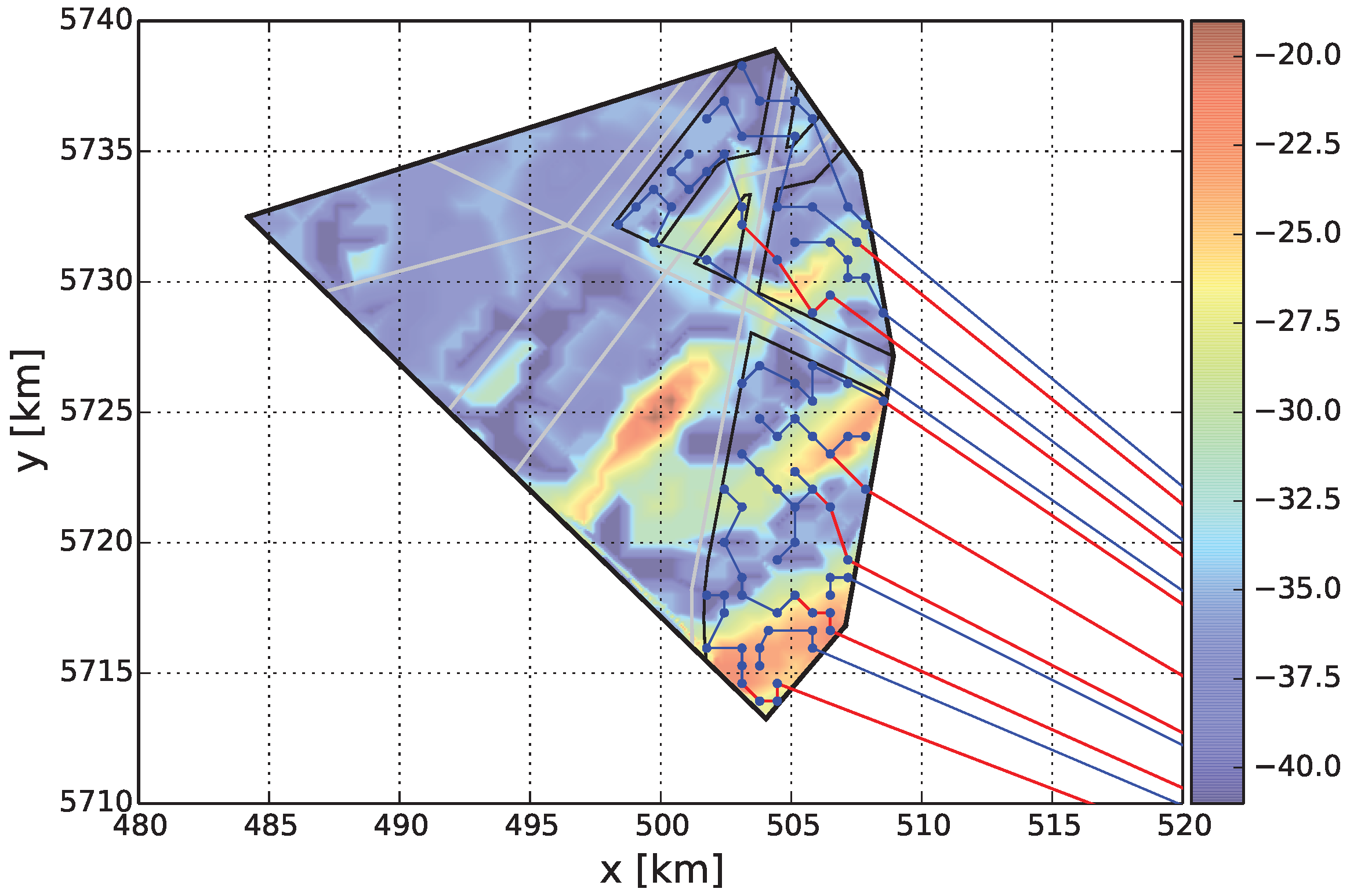
6.2. Wind Farm Layouts Designed with Standard Approaches

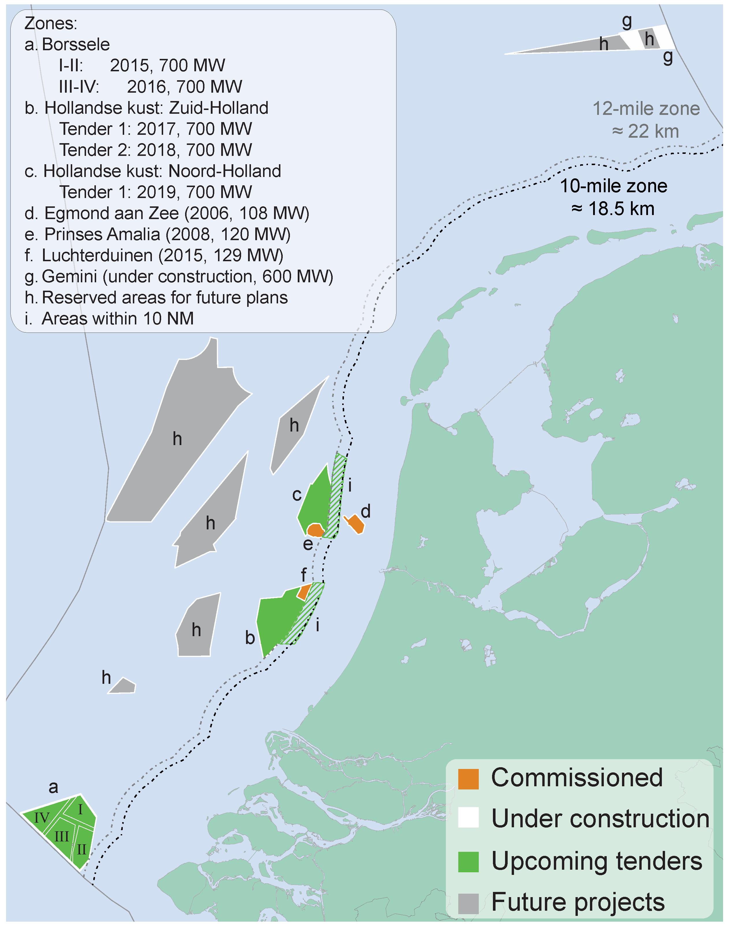
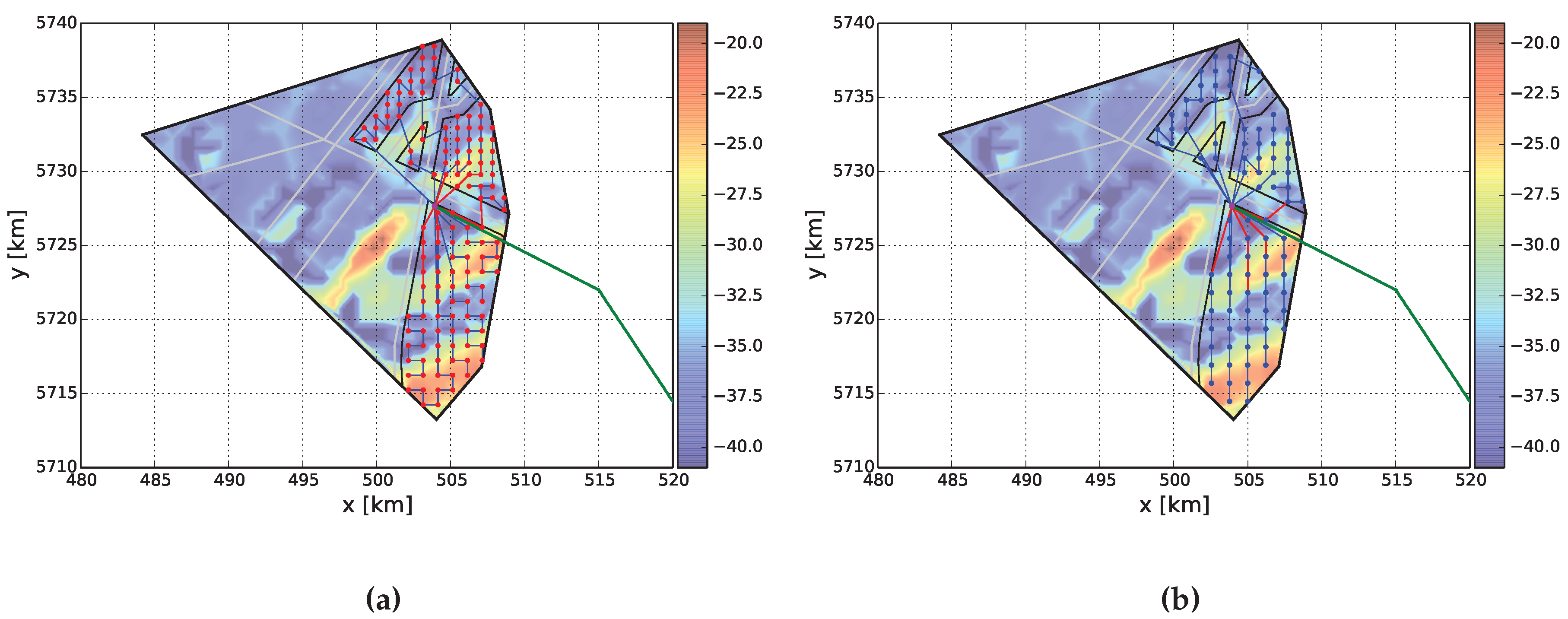
Two OWF layouts were hand-designed by taking into consideration the guidelines given to these areas [134]. In this way, 350 MW (352 MW for the 8 MW turbines) were placed in each wind farm area and all the turbines were interconnected to one 220 kV HVac offshore substation placed in the exact location where it will be built [
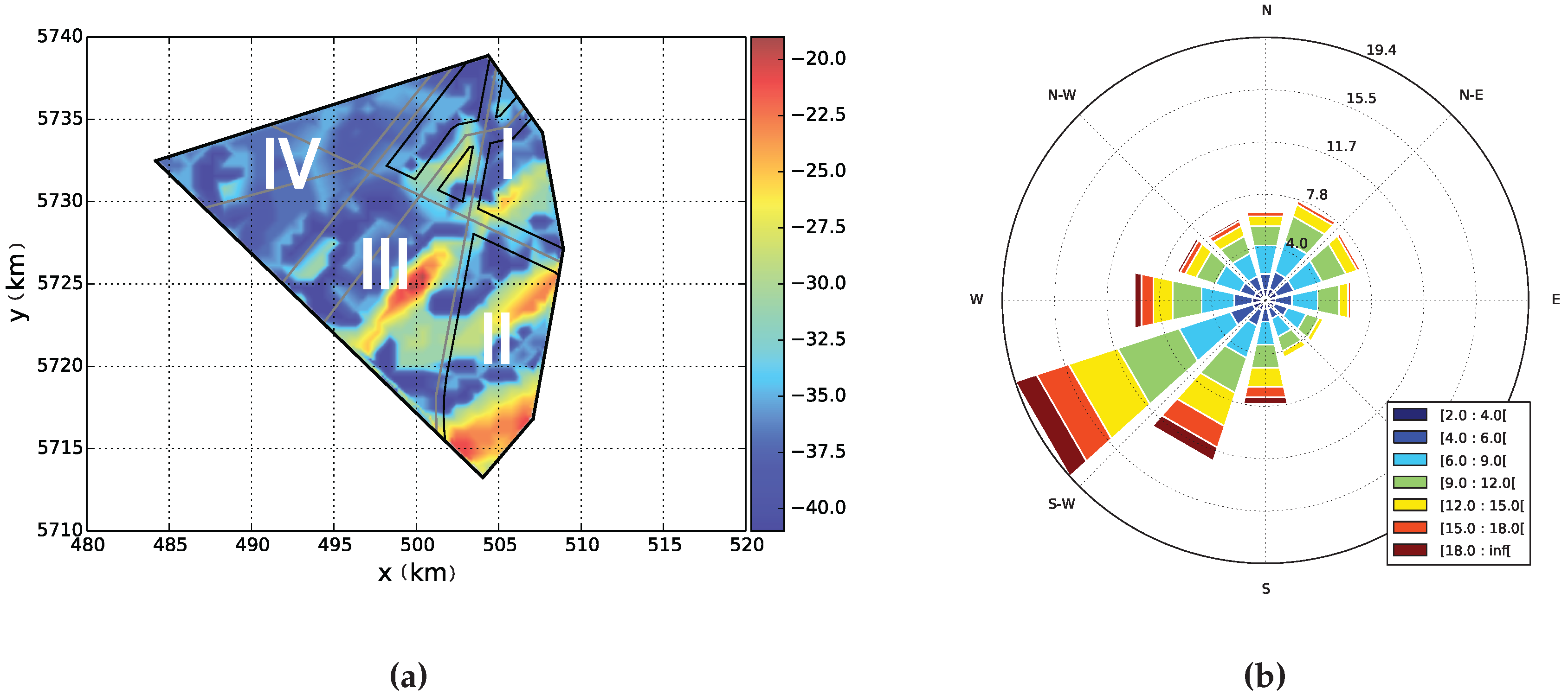
83]. It is important to note that some level of optimization was used during the design of these layouts. The wind turbines were placed in the grid that maximized the distance between them. Furthermore, as shown in Figure 17, the turbines have a larger distance between them in the main wind direction (see Figure 12b). The collection systems were designed with the heuristic algorithm presented in [75].
The grid step sizes used in the standard layouts are different from the ones that the optimization framework had access to. This difference may explain why no layouts that export the power to shore via HVac technology were found in the vicinity of the trade-off (see Section 3.1) shown in Figure 16. Nonetheless, the layout with 8 MW wind turbines did not dominate (was not superior in any way) the layouts of the optimized trade-off.

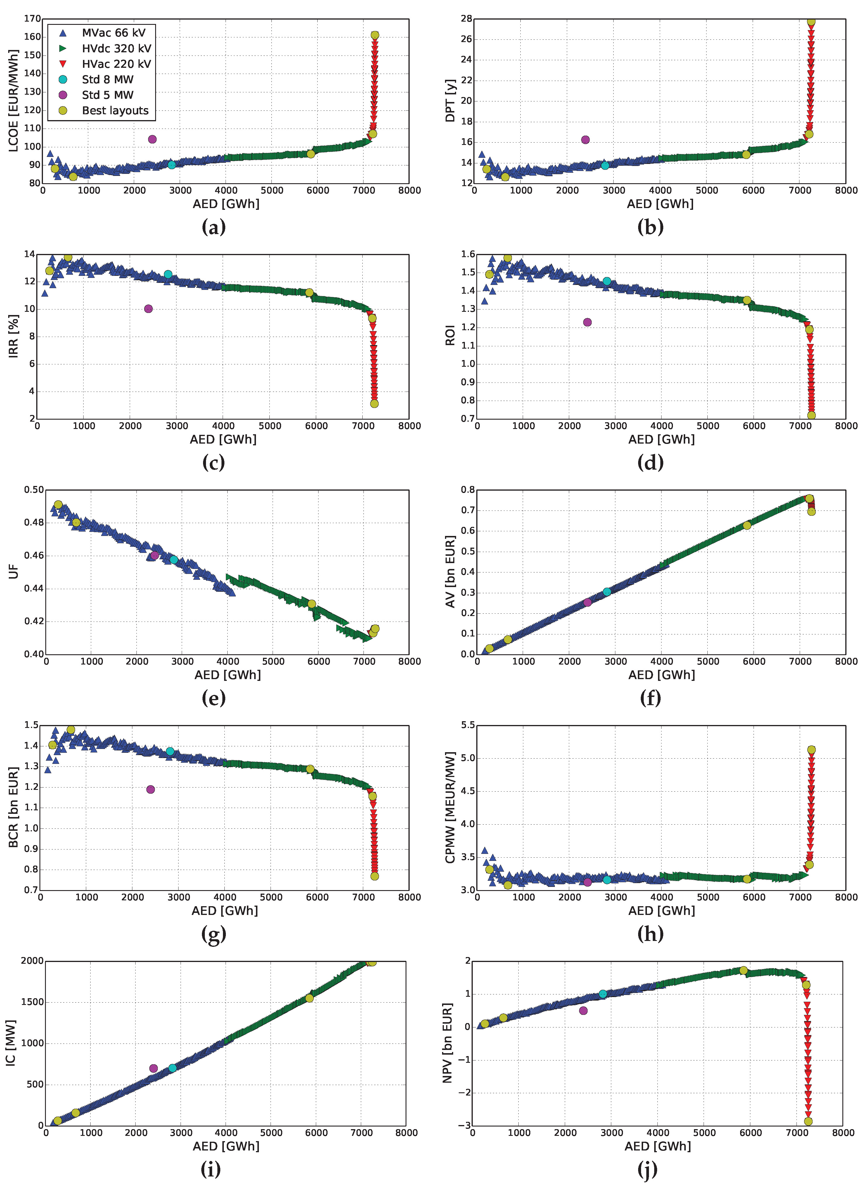
6.3. Economic Functions

Figure 18 shows how the layouts of the optimized trade-off perform according to the economic functions presented in Table 3. 
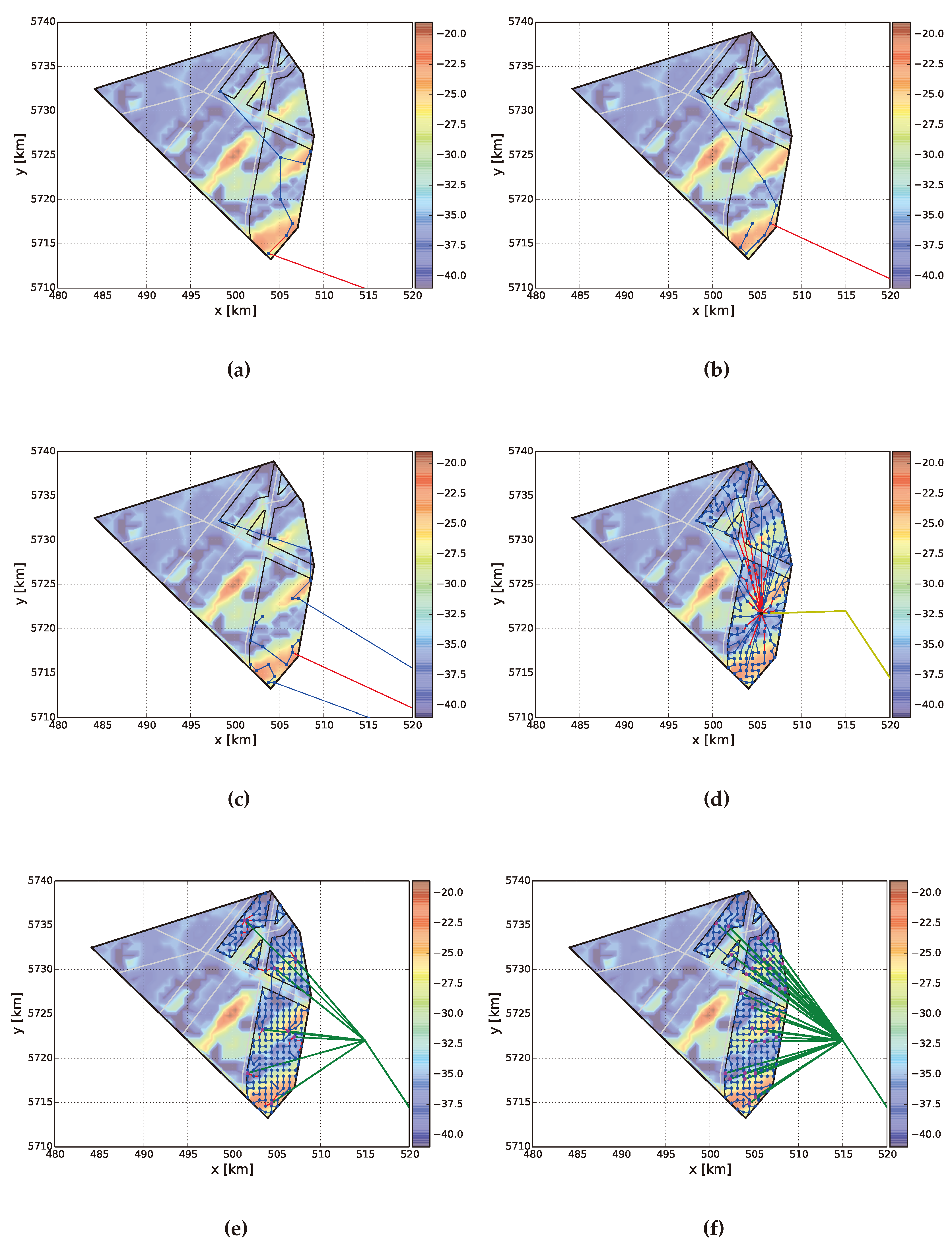
Table 8 presents the economic values and general characteristics of the layouts (shown in Figure 19) that demonstrated to be the best according to the different economic functions. The results were obtained with the following assumptions: interest rate of 7% [70], wind farm lifetime of 20 years, annual OPEX of 2% of the respective CAPEX [44,45,135] and price of energy of 0.124 €/kWh, which is the highest bid for the Borssele areas I and II [83]. In Section 6.4 the impact of these parameters will be assessed. Although fixed annual values were used, distinct annual values could have been applied in a straightforward manner to simulate, for example, the financial incentives that the energy generated at OWFs obtain in the first years of exploration [136]. However, these incentives are country specific and, therefore, were not considered.

6.3.1. AED

Figure 19f shows the layout with the highest AED, whereas some of its characteristics are given in Table 8. The layout uses the concept of distributed substations in which several small offshore substations housing a single transformer and one reactor for compensation of the export cable are used [137]. This concept, as shown in Figure 19f and Table 8, leads to a significant reduction in the total collection system length (CSL) since this layout has 110 km less array cables than layout number 248, which has 55 turbines less. The electrical losses are reduced and the usage of array cables with high cross sections is also minimized in layout number 358. Furthermore, this concept leads to fewer crossings with existing pipelines and telecom cables as shown in Figure 19f. On average, there are approximately nine turbines (72 MW) connected to each substation.
The AED function is fully biased towards energy production maximization, hence, designers should be cautious when applying it in case there are no constraints over the installed power or a maximum project CAPEX. Moreover, the economic values obtained for this layout clearly demonstrated that. This layout obtained a negative NPV, a DPT of almost 28 years and a ROI value lower than one, meaning that the investment would not be able to generate profit for the wind farm developers, despite its very high AED.

6.3.2. Utilization Factor

The layout which presented the highest UF value, shown in Figure 19a, was composed of only eight 8-MW turbines. Since the objective is to minimize the losses one might initially think that a layout with only one turbine would provide the best results. However not only the wake losses are being considered but all the power losses until the PCC. In this way, the layout with eight turbines demonstrated to also make a better use of the MVac cable. The turbines were placed far apart from each other and in shallow areas. The same layout would present the best result if the efficiency of the system would have been used instead of the UF [33].
The standard layout with 5-MW turbines presented worse results than its counterpart composed of Vestas turbines in all function but the UF. This means that despite the lower AED, the 5-MW turbines are slightly better used and it would be in the preferred layout if the UF was the most important decision factor.

6.3.3. LCOE

The LCOE values of the optimized layouts are shown in Figure 18a. Values between approximately 80 to 105 €/MWh were found for MVac and HVdc transmission technologies. On the other hand, the layouts based on HVac technology presented much higher LCOE values due to their higher investment costs than the other layouts which used HVdc and MVac transmission systems.
The layout which presented the lowest LCOE (83.79 €/MWh) was composed of 20 turbines as shown in Figure 19c. Although the turbines were placed far apart to minimize wake losses, they were also placed in regions of shallow waters to minimize the cost of support structures. Furthermore, the turbines were also placed in the wind farm area closest to shore, minimizing the cabling system cost and the electrical losses.

6.3.4. IRR, ROI, COP, BCR and DPT

The same layout that had the lowest LCOE also presented the best values for the IRR, DPT, COP, BCR and ROI functions. Although these economic indicators present different values, they did not alter the ranking between layouts, i.e., if a certain layout performs best at one of these economic functions it also turns out to be the best according to the remaining ones.

6.3.5. AV

The AV equation is biased towards larger wind farms since it measures the annual revenue. The layout that maximized the AV equation is shown in Figure 19e and it is very similar to layout number 358, shown in Figure 19f. The only difference is that it makes use of eight offshore HVac substations to interconnect the 249 turbines to shore.

6.3.6. Incremental BCR

According to the incremental BCR economic analysis, the wind farm layout number 5 (see Figure 19b) was the preferred choice. It is composed of ten 8 MW turbines and, therefore, makes full use of the 66 kV cable with the largest cross section (see Table 5), thus minimizing the ratio between the AED and the investment costs.

6.3.7. NPV

The wind farm layout which presented the highest NPV value (Figure 19d) has one HVdc offshore substation that interconnects 194 turbines to shore.

6.4. The Influence of Economic Factors

In this section, the influence of the economic factors over the wind farm layout design is investigated. To this end, different parameters, such as the interest rate, wind farm lifetime and price of energy, were altered to analyze the resulting implications. Initially the LCOE will be analyzed, followed by the NPV function.
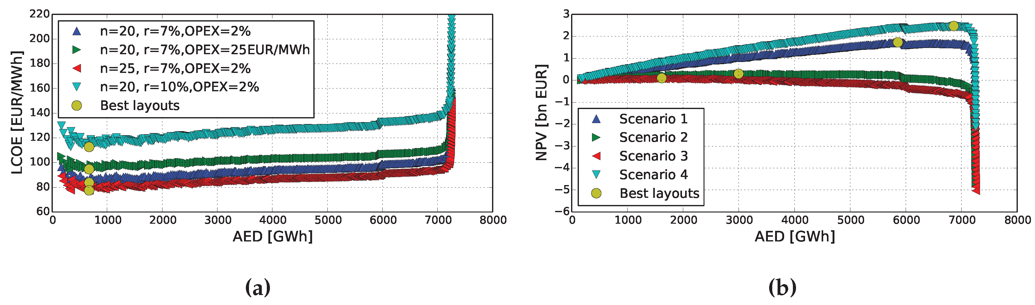
6.4.1. LCOE

Assuming the OPEX to be a percentage of the investment costs [44,45], p C A P E X , the LCOE clearly becomes a ratio between the CAPEX and the AED:
L C O E = C A P E X A E D 1 a + p C A P E X
This equation shows that both an alteration to the interest rate and wind farm lifetime or a different percentage of the CAPEX for the OPEX, will affect in the same way all the wind farm layouts since it only shifts the ratio between the CAPEX and the AED.
Another possibility, in the absence of a more refined OPEX model, is to monetize the OPEX through a cost value per MWh, c, delivered by the OWF [49,120]:
L C O E = 1 A E D C A P E X a + c · A E D = C A P E X a · A E D + c
Once again, all the layouts will be affected in the same way if the value c is changed. This means that, if the OPEX is somewhat directly dependent on either the CAPEX or the AED, the LCOE function is insensitive to the variation of its economic factors. Figure 20a shows that the order of the layouts of the optimized trade-off remained unaltered, hence, the wind layout number 18 remained the one with the lowest LCOE value.

6.4.2. NPV

Different from the LCOE function, the variation of the economic parameters will influence differently the cash flows of the NPV equation even if the OPEX is proportional to one of the other goals (see Figure 20b). In this way, the economic parameters play an important role as weighting factors in the outcome of the NPV function. Table 9 presents the characteristics of the four layouts (shown in Figure 21) with the highest NPV value for different economic parameters and shows the layouts.
If the designers used an energy price of 0.1 €/kWh, which is the target for energy generated offshore by 2020 (see Section 1), a layout with an IC of 752 MW presents the highest NPV (see Figure 21b). This is the only layout of the optimized trade-off curve that has a similar capacity to the 700-MW guideline which demonstrated to be advantageous at some point.
If the lifetime operation of the OWF is considered to be 25 years [138,139], it is more beneficial, according to the NPV function, to install more turbines to increase the AED and take advantage of the extra time of operation (Figure 21d).
Figure 20b demonstrates that the higher the revenues, either through a higher price of energy or via a longer exploration of the site, the NPV function is maximized with OWFs with higher installed capacities (IC). If the revenues are lower, wind farms with less turbines present the highest NPV values.

6.5. Discussion

The optimized trade-off curve was obtained in 30 days with the proposed framework, which is relatively fast if compared to the design phase of a state-of-the-art OWF which takes several months [140]. The optimization strategy also demonstrates that designers would have missed other wind farm designs that could lead to similar AED and CAPEX values. For example, Figure 22 shows a layout with 88 Vestas 8 MW turbines connected to shore via 66-kV cables, which has similar values for the AED and CAPEX as the standard layout of Figure 17b. If, for example, there would be a risk associated with building structures offshore (e.g., substations, or reliability values for the different components of the system), the layout obtained with the algorithm would be preferable to the standard HVac-based one.
No high-level constraints were applied to the case study, e.g., maximum installed capacity. Although these will have an influence on the choice of the layout, the basis of the framework holds since the designers are only required to firstly discard the layouts which do not meet the high-level constraints and then apply the economic functions over the remaining ones.
The optimization phase itself can still be an iterative process of refining the optimization goals and constraints because the MO algorithm is powerful enough to exploit peculiarities in an optimization goal that actually still gives undesired results. For example, in the case study there was no restriction regarding the maximum number of export cables or a preference towards layouts which used offshore substations. In this way, even though the layouts shown in Figure 17b and Figure 22 have similar AED and CAPEX values, the latter, found with the optimization framework, may not be desired by the wind farm designers due to the high amount of cables connected to shore. On the other hand, the layout of Figure 22 does not require offshore substations, which if a certain level of risk is associated to them, may represent an advantage over the layout shown in Figure 17b.
The proposed MO optimization framework provides the designers with important information that could not easily be obtained with single-objective alternatives. For example, the optimized trade-off shown in Figure 16 shows to the designers the best transmission technology and voltage level for the different range of installed capacities. Furthermore the trade-off also informs the designers to any possible important point of transition in the problem design space, i.e., it shows when increasing the installed capacity does not lead to better designs but solely to more expensive layouts. For example, this is the case for the right part of the optimized trade-off of Figure 16. Even though the layouts have higher AED, this comes with a dramatic increase of the CAPEX. Therefore, this alerts the designers that such layouts do not represent the best layouts.
The discovery of important points of transition in the problem search space (Figure 16) is also directly applicable in other search spaces, such as the economic functions shown in Figure 18. The designers are informed when the layouts do not present interesting economic figures in a straightforward manner.
The multi-objective optimization approach also provides the designers with wind farm designers that were optimized without using economic parameters. This allows the designers to iterate over the different layouts with different economic parameters without the need to rerun the optimization (see Section 6.4).

7. Conclusions

A review of existing commercial and academic optimization tools showed their drawbacks and gaps to be twofold: first, the optimization processes are based on a sequential approach and, second, a priori economic assumptions need to be made for the optimization phase. To solve these issues, a MO optimization framework to automate, integrate and optimize the design of OWFs was presented in this work.
The design aspects of existing offshore wind farms, e.g., number and location of offshore substations and collection system design, were analyzed. Furthermore, also the industrial trends of the components was investigated. In this way, it was assured that the optimization framework captures all the important design aspects and the industrial trends of the components used in state-of-the-art offshore wind farm. Also, the important optimization variables of the wind farm layout optimization problem were assessed.
A state-of-the-art multi-objective optimization algorithm, so-called MOGOMEA, was used in this work. More specifically, a variant of the algorithm tailored for the wind farm layout optimization problem was employed. The algorithm and the optimization framework were then applied to a case study in the Dutch offshore Borssele area. The framework found several wind farm layouts that represent an optimized trade-off of between the design goals, the annual energy delivered to the onshore electrical network and the investment costs.
Distinct wind farm layouts demonstrated to be the most profitable choice depending on the economic function used. The economic factors, e.g., interest rate and price of energy, demonstrated to play an important role in the outcome of the best layout. These results show that wind farm designers should not decide the layout of the wind farm based solely on one economic function such as the NPV or LCOE. Instead, designers should carefully inspect the performance of the layouts at hand using several economic functions.
The proposed framework helps the designers to perform such analysis since all efficient trade-offs are presented to them. This way, designers may iterate over the optimized trade-offs to select which layout is the most suitable without rerunning the optimization tool, accelerating the decision phase and reducing costs. Moreover, the framework designed layouts that performed similarly to layouts based on existing design strategies, e.g., placement of turbines in a standard grid. This result indicates that designers may be missing other design concepts that lead to similar performances. Nonetheless, the selection of the wind farm layout has to undergo a selection to assure that it is the one that most meets the desire of the designers.

Acknowledgments

The work was done within the project “Far and Large Offshore Wind (FLOW)”, which is supported by the Ministry of Economic Affairs, Agriculture and Innovation of the Netherlands within the EOS-LT program of Agentschap-NL (P201101-005-ECN). The opinion expressed by the authors does not necessarily reflect the position of the Ministry of Economic affairs, nor does it involve any responsibility on its part. The work was also performed under the Funding Agency Grant CONICYT-FONDECYT 11150069. The authors would like to thank the Het Collectief company for providing the computational resources used to obtain the results presented in this paper.

Author Contributions

All authors were involved during the development of the manuscript. S. Rodrigues wrote the article and was in charge of most of the modeling. G. Katsouris wrote the heuristic to design the collection systems, R. Teixeira Pinto wrote the code to compute the power flows and P. Bosman designed the multi-objective optimization algorithm. C. Restrepo contributed with the illustrations present in the work and provided general input during the writing of this work. M. Soleimanzadeh and P. Bauer provided valuable insights throughout the research and writing processes.

Conflicts of Interest

The authors declare no conflict of interest.

Abbreviations

AED (GWh/year)Annual Energy Delivered
AEP (GWh/year)Annual Energy Production
AV (bn €)Annualized Value
BCR [–]Benefit to Cost Ratio
CAPEX (bn €)Capital Expenditure
COE (M€/MWh)Cost of Energy
COP (M€/MW)Cost of Power
CSL (km)Collection System Length
DCODevelopment Consent Order
DFIGDoubly-Fed Induction Generator
DPT (years)Discounted Payback Time
FEEDFront-End Engineering and Design
HVacHigh-Voltage alternate current
HVdcHigh-Voltage direct current
IC (MW)Installed Capacity
IRR (%)Internal Rate of Return
LCOE (€/MWh)Levelized Cost of Energy
MMCModular Multi-level Converter
MOMulti-Objective
MOGOMEAMulti-Objective Gene-pool Optimal Mixing Evolutionary Algorithm
MVacMedium-Voltage alternate current
NPV (bn €)Net Present Value
NSSNumber of Substations
OPEX (bn €)Operational Expenditure
OWFOffshore Wind Farm
PCCPoint of Common Coupling
PMSGPermanent-Magnet Synchronous Generator
RD (m)Rotor Diameter
ROI [–]Return on Investment
TTTransmission Technology
UXOUneXploded Ordnance
UF [–]Utilization Factor
VSCVoltage-Source Converter
WFLOPWind Farm Layout Optimization Problem

References

  1. Christensen, B. The road to below 10 ct EUR/kWh—Siemens response to the challenge. In Proceedings of the EWEA (European Wind Energy Association) Offshore 2015, Copenhagen, Denmark, 10–12 March 2015.
  2. BVG Associates. Future Renewable Energy Costs: Offshore Wind—How Technology Innovation Is Anticipated to Reduce the Cost of Energy from European Offshore Wind Farms; Technical Report; KIC InnoEnergy: Eindhoven, The Netherlands, 2014. [Google Scholar]
  3. The Crown Estate. Offshore Wind Cost Reduction—Pathways Study. Technical Report. Available online: http://www.thecrownestate.co.uk/energy-and-infrastructure/offshore-wind-energy/working-with-us/strategic-workstreams/cost-reduction-study/ (accessed on 15 March 2016).
  4. Offshore Wind Cost Reduction Task Force. Offshore Wind Cost Reduction Task Force Report; Technical Report. Available online: https://www.gov.uk/government/groups/offshore-wind-cost-reduction-task-force (accessed on 15 March 2016).
  5. Offshore Renewable Energy Catapult. Cost Reduction Monitoring Framework. Technical Report. Available online: https://ore.catapult.org.uk/documents/10619/168655/pdf/a8c73f4e-ba84-493c-8562-acc87b0c2d76 (accessed on 15 March 2016).
  6. Offshore Wind Programme Board. Sharing Good Practice in the Supply Chain to Facilitate Cost Reduction; Technical Report Rev 03; The Crown Estate: London, UK, 2012. [Google Scholar]
  7. Milborrow, D. Onshore wind is more competitive than ever. Available online: http://www.windpowermonthly.com/article/1330525/onshore-wind-competitive-ever (accessed on 15 March 2016).
  8. The Wind Power. EWEA Offshore: Offshore to be cost competitive by 2023. Available online: http://www.windpowermonthly.com/article/1337352/ewea-offshore-offshore-cost-competitive-2023 (accessed on 1 June 2015).
  9. DNV GL. Project FORCE—Offshore Wind Cost Reduction through Integrated Design; Technical Report; DNV GL: Hovik, Norway, 2014. [Google Scholar]
  10. Lindoe Offshore Renewables Center. List of Offshore Wind Farms. Available online: http://www.lorc.dk/offshore-wind-farms-map/list (accessed on 1 March 2015).
  11. 4C Offshore. Offshore Wind Farms. Available online: www.4coffshore.com/windfarms (accessed on 23 March 2015).
  12. Trading Economics. Available online: http://www.tradingeconomics.com/euro-area/inflation-cpi (accessed on 8 August 2015).
  13. BVG Associates. Value Breakdown for the Offshore Wind Sector; Technical Report; Renewables Advisory Board: Eindhoven, The Netherlands, 2010. [Google Scholar]
  14. Scottish Enterprise. Offshore Wind Fact Overview of a Wind Farm Project; Technical Report; Scottish Enterprise: Glasgow, Scotland, 2010. [Google Scholar]
  15. Galloper Wind Farm Limited. Galloper Wind Farm Project Environmental Statement—Chapter 5 Project Details; Technical Report; RWE Innogy and SSE Group: Wiltshire, UK, 2011. [Google Scholar]
  16. Galloper Wind Farm Limited. Gwynt y Mor Offshore Wind Farm—Environmental Statement (Non Technical Summary); Technical Report; RWE Innogy and SSE Group: Wiltshire, UK, 2005. [Google Scholar]
  17. Ebbesen, M.C. Seeing the big picture—Finding the optimal conceptual design. In Proceedings of the EWEA (European Wind Energy Association) Offshore 2015, Copenhagen, Denmark, 10–12 March 2015.
  18. Esteban, M.D.; Lopez-Gutierrez, J.S.; Diez, J.J.; Negro, V. Methodology for the design of offshore wind farms. In Proceedings of the 11th International Costal Symposium, Szczecin, Poland, 9–14 May 2011.
  19. European Wind Energy Association. Wind Energy—The Facts Part I Technology; Technical Report; Wind Energy: Brussels, Belgium, 2009. [Google Scholar]
  20. Clausen, R.S. Optimising wind farm layouts—Weighing costs against benefits. In Proceedings of the EWEA (European Wind Energy Association) Offshore 2015, Copenhagen, Denmark, 10–12 March 2015.
  21. Wyatt, S.; Govindji, A.K.; James, R.; Duan, N.; Xie, B.; Liu, M.; Yi, G. Detailed Appraisal of the Offshore Wind Industry in China; Technical Report; Carbon Trust: London, UK, 2014. [Google Scholar]
  22. Rodrigues, S.; Restrepo, C.; Kontos, E.; Pinto, R.T.; Bauer, P. Trends of offshore wind projects. Renew. Sustain. Energy Rev. 2015, 49, 1114–1135. [Google Scholar] [CrossRef]
  23. Rheinisch-Westfalisches Elektrizitatswerk. Gwynt y Mor Offshore Wind Farm Key Statistics. Available online: https://www.rwe.com/web/cms/en/1252456/rwe-innogy/sites/wind-offshore/under-construction/gwynt-y-mr/tech-and-spec/ (accessed on 31 March 2015).
  24. Lumbreras, S.; Ramos, A. Offshore wind farm electrical design: A review. Wind Energy 2013, 16, 459–473. [Google Scholar] [CrossRef]
  25. Herbert-Acero, J.F.; Probst, O.; Rethore, P.E.; Larsen, G.C.; Castillo-Villar, K.K. A Review of Methodological Approaches for the Design and Optimization of Wind Farms. Energies 2014, 7, 6930–7016. [Google Scholar] [CrossRef]
  26. Tong, W.; Chowdhury, S.; Mehmani, A.; Messac, A. Multi-Objective wind farm design—Exploring the trade-off between capacity factor and land use. In Proceedings of the 10th World Congress on Structural and Multidisciplinary Optimization, Orlando, FL, USA, 19–24 May 2013.
  27. Khan, S.; Rehman, S. Computational intelligence techniques for placement of wind turbines: A brief plan of research in Saudi Arabian perspective. In Proceedings of the 2010 IEEE International Energy Conference and Exhibition (EnergyCon), Manama, Bahrain, 18–22 December 2010; pp. 519–523.
  28. Kusiak, A.; Song, Z. Design of wind farm layout for maximum wind energy capture. Renew. Energy 2010, 35, 685–694. [Google Scholar] [CrossRef]
  29. Zhang, P.Y. Topics in Wind Farm Layout Optimization: Analytical Wake Models, Noise Propagation, and Energy Production. Master’s Thesis, University of Toronto, Toronto, ON, Canada, 2013. [Google Scholar]
  30. Kwong, W.Y.; Zhang, P.Y.; Romero, D.; Moran, J.; Morgenroth, M.; Amon, C. Wind farm layout optimization considering energy generation and noise propagation. In Proceedings of the ASME 2012 International Design Engineering Technical Conferences & Computers and Information in Engineering Conference, Chicago, IL, USA, 12–15 August 2012.
  31. Veeramachaneni, K.; Wagner, M.; O’Reilly, U.M.; Neumann, F. Optimizing energy output and layout costs for large wind farms using particle swarm optimization. In Proceedings of the IEEE Congress on Evolutionary Computation, Brisbane, Australia, 10–15 June 2012; pp. 1–7.
  32. Tran, R.; Wu, J.; Denison, C.; Ackling, T.; Wagner, M.; Neumann, F. Fast and effective multi-objective optimisation of wind turbine placement. In Proceedings of the 15th Annual Conference on Genetic and Evolutionary Computation, Amsterdam, The Netherlands, 6–10 July 2013; pp. 1381–1388.
  33. Rodrigues, S.; Bauer, P.; Bosman, P.A. Multi-Objective Optimization of Wind Farm Layouts—Complexity, Constraint Handling and Scalability. Renew. Sustain. Energy Rev. 2016. submitted. [Google Scholar]
  34. Sorkhabi, S.; Romero, D.; Beck, J.; Amon, C. Constrained multi-objective wind farm layout optimization—Introducing a novel constraint handling approach based on constraint programming. In Proceedings of the International Design Engineering Technical Conference, Boston, MA, USA, 2–5 August 2015.
  35. Sisbot, S.; Turgut, O.; Tunc, M.; Camdali, U. Optimal positioning of wind turbines on Gokceada using multi-objective genetic algorithm. Wind Energy 2010, 13, 297–306. [Google Scholar] [CrossRef]
  36. WindPRO; EMD International A/S: Aalborg, Denmark. Available online: http://www.emd.dk/WindPRO (accessed on 20 April 2014).
  37. GHWindFarmer. Available online: http://www.gl-garradhassan.com/en/software/GHWindFarmer.php (accessed on 20 April 2014).
  38. Wind Resources for Wind Turbine Production. Wind resources for energy production of wind turbines. Available online: http://www.wasp.dk/wasp (accessed on 20 April 2014).
  39. OpenWind; AWS Truepower: Albany, NY, USA. Available online: http://www.awstruepower.com/solutions/products/openwind/ (accessed on 20 April 2014).
  40. WindSim. Available online: http://www.windsim.com/ (accessed on 20 April 2014).
  41. ReSoft. Wind Farm Analysis, Design and Optimisation. Available online: http://www.resoft.co.uk/ (accessed on 20 April 2014).
  42. Kallioras, N.A.; Lagaros, N.D.; Karlaftis, M.G.; Pachy, P. Optimum layout design of onshore wind farms considering stochastic loading. Adv. Eng. Softw. 2015, 88, 8–20. [Google Scholar] [CrossRef]
  43. Song, M.; Chen, K.; Zhang, X.; Wang, J. Optimization of wind turbine micro-siting for reducing the sensitivity of power generation to wind direction. Renew. Energy 2016, 85, 57–65. [Google Scholar] [CrossRef]
  44. Elkinton, C.N.; Manwell, J.F.; McGowan, J.G. Offshore wind farm layout optimization (OWFLO) project: An introduction. In Proceedings of the European Offshore Wind Conference & Exhibition, Copenhagen, Denmark, 26–28 October 2005.
  45. Lackner, M.A.; Elkinton, C.N. An Analytical Framework for Offshore Wind Farm Layout Optimization. Wind Eng. 2007, 31, 17–31. [Google Scholar] [CrossRef]
  46. Gribben, B.J.; Williams, N.; Ranford, D. Offshore wind farm layout design—A systems engineering approach. In Proceedings of the Ocean Power Fluid Machinery, London, UK, 19 October 2010.
  47. Rethore, P.E.; Fuglsang, P.; Larsen, G.; Buhl, T.; Larsen, T.; Madsen, H. TopFarm: Multi-fidelity optimization of offshore wind farm. In Proceedings of the ISOPE (International Society of Offshore and Polar Engineers) Conference, Maui, HI, USA, 19–24 June 2011.
  48. Short, W.; Packey, D.J.; Holt, T. A Manual for the Economic Evaluation of Energy Efficiency and Renewable Energy Technologies; Technical Report NREL/TP-462-5173; National Renewable Energy Laboratory: Golden, CO, USA, 1995. [Google Scholar]
  49. Elkinton, C.N. Offshore Wind Farm Layout Optimization. Ph.D. Thesis, University of Massachusetts, Amherst, MA, USA, 2007. [Google Scholar]
  50. de Oliveira, W.S.; Fernandes, A.J. Investment Analysis For Wind Energy Projects. Rev. Bras. Energ. 2013, 19, 239–285. [Google Scholar]
  51. Erlich, I.; Shewarega, F.; Feltes, C.; Koch, F.; Fortmann, J. Offshore Wind Power Generation Technologies. Proc. IEEE 2013, 101, 891–905. [Google Scholar] [CrossRef]
  52. Project Management Support Services Ltd (PMSS). Greater Gabbard Offshore Wind Farm Non Technical Summary; Technical Report; Greater Gabbard Offshore Winds Ltd.: Wiltshire, UK, 2005. [Google Scholar]
  53. European Wind Energy Association. The European Offshore Wind Industry—Key Trends and Statistics 2013; Technical Report; Wind Energy: Brussels, Belgium, 2014. [Google Scholar]
  54. Countries list, The Wind Power. Available online: http://www.thewindpower.net/windfarms_offshore_en.php (accessed on 1 March 2015).
  55. Polinder, H.; Ferreira, J.; Jensen, B.; Abrahamsen, A.; Atallah, K.; McMahon, R. Trends in Wind Turbine Generator Systems. IEEE J. Emerg. Sel. Top. Power Electron. 2013, 1, 174–185. [Google Scholar] [CrossRef]
  56. Teixeira Pinto, R.; Rodrigues, S.; Bauer, P.; Pierik, J. Grid code compliance of VSC-HVDC in offshore multi-terminal DC networks. In Proceedings of the 39th Annual Conference of the IEEE Industrial Electronics Society, Vienna, Austria, 10–13 November 2013.
  57. Ibsen, L.B.; Liingaard, M.; Nielsen, S.A. Bucket Foundation, a status. In Proceedings of the Copenhagen Offshore Wind, Copenhagen, Danmark, 26–28 October 2005.
  58. de Villiers, P. Demonstrating Keystone Engineering’s Innovative Inward Battered Guide Structure (IBGS) Offshore Foundation Concept at Hornsea—Best Practice for Private-Public Cooperation; Technical Report; Carbon Trust: London, UK, 2012. [Google Scholar]
  59. Gengenbach, J.; Mikkelsen, K.; Rudinger, F.; Brommundt, M.; Gretlund, J.S. Design challenges of XL monopiles. In Proceedings of the EWEA (European Wind Energy Association) Offshore 2015, Copenhagen, Denmark, 10–12 March 2015.
  60. Govindji, A.K.; James, R.; Carvallo, A. Appraisal of the Offshore Wind Industry in Japan, Technical Report; Carbon Trust: London, UK, 9 October 2014.
  61. European Wind Energy Assoctiation. Deep Water—The Next Step for Offshore Wind Energy; Technical Report; European Wind Energy Association: Brussels, Belgium, 2013. [Google Scholar]
  62. Roddier, D.; Cermelli, C.; Aubault, A.; Weinstein, A. WindFloat: A floating foundation for offshore wind turbines. Renew. Sustain. Energy 2010, 2, 1–34. [Google Scholar] [CrossRef]
  63. Japan’s floating offshore wind projects: An overview; Technical Report; Main(e) International Consulting LLC: Bremen, ME, USA, 2013.
  64. Floating Offshore Wind Foundations: Industry Consortia and Projects in the United States, Europe and Japan—An Overview; Technical Report; Main(e) International Consulting LLC: Bremen, ME, USA, 2013.
  65. Sorensen, T.; Thogersen, M.L.; Nielsen, P. Adapting and Calibration of Existing Wake Models to Meet the Conditions Inside Offshore Wind Farms; Technical Report; EMD International A/S: Aalborg, Denmark, 2008. [Google Scholar]
  66. The Crown Estate. Submarine Cables and Offshore Renewable Energy Installations—Proximity Study; Technical Report; The Crown Estate: London, UK, 2012. [Google Scholar]
  67. Rodrigues, S.; Bauer, P.; Pierik, J. Comparison of offshore power transmission technologies: A multi-objective optimization approach. In Proceedings of the 15th International Power Electronics and Motion Control Conference (EPE/PEMC), Novi Sad, Serbia, 4–6 September 2012.
  68. Schachner, J. Power Connection for Offshore Wind Farms. Master’s Thesis, Delft University of Technology, Delft, The Netherlands, 2004. [Google Scholar]
  69. Carbon Trust. Offshore Wind Accelerator—Driving Down the Cost of offshore Wind. Available online: http://carbontrust.com/media/105322/electrical_presentation_jm_-dec_2011.pdf (accessed on 1 May 2014).
  70. Pierik, J.; Pavlovsky, M.; Bozelie, J.; Bauer, P.; de Haan, S. Dowec Electrical System Baseline Design; Technical Report DOWEC 045 Rev. 2; Energy Research Centre of the Netherlands (ECN): Petten, The Netherlands, 2002. [Google Scholar]
  71. Berzan, C.; Veeramachaneni, K.; McDermott, J.; O’Reilly, U.M. Algorithms for Cable Network Design on Large-Scale Wind Farms; Technical Report; Tufts University: Medford, MA, USA, 2011. [Google Scholar]
  72. Bauer, J.; Lysgaard, J. The offshore wind farm array cable layout problem: A planar open vehicle routing problem. J. Op. Res. Soc. 2014, 66, 360–368. [Google Scholar] [CrossRef]
  73. Tesauro, A.; Rethore, P.E.; Larsen, G. State of the art of wind farm optimization. In Proceedings of EWEA—European Wind Energy Conference & Exhibition, Copenhagen, Denmark, 16–19 April 2012.
  74. Dicorato, M.; Forte, G.; Pisani, M.; Trovato, M. Guidelines for assessment of investment cost for offshore wind generation. Renew. Energy 2011, 36, 2043–2051. [Google Scholar] [CrossRef]
  75. Katsouris, G. Infield Cable Topology Optimization of Offshore Wind Farms. Master’s Thesis, Delft University of Technology, Delft, The Netherlands, 2015. [Google Scholar]
  76. Papadopoulos, A. Modeling of Collection and Transmission Losses of Offshore Wind Farms for Optimization Purposes. Master’s Thesis, Delft University of Technology, Delft, The Netherlands, 2015. [Google Scholar]
  77. Teixeira Pinto, R. Multi-Terminal dc Networks—System Integration, Dynamics and Control. Ph.D. Thesis, Delft University of Technology, Delft, The Netherlands, 2014. [Google Scholar]
  78. Rodrigues, S. Dynamic Modeling and Control of VSC-based Multi-Terminal DC Networks. Master’s Thesis, Instituto Superior Técnico, Lisbon, Portugal, 2011. [Google Scholar]
  79. Donat, L.; Eberle, A.; Velten, E.K.; Prahl, A.; Wevers, M. Assessment of Climate Change Policies in the Context of the European Semester—Country Report The Netherlands; Technical Report; Ecologic Institute and Eclareon: Berlin, Germany, 2014. [Google Scholar]
  80. Loyens and Loeff. North Sea offshore wind—Developments in Belgium and the Netherlands; Technical Report; Rotterdam, The Netherlands, 2014. [Google Scholar]
  81. Netherlands Enterprise Agency. North Sea 2050 Spatial Agenda; Technical Report; Ministerie van Economische Zaken: The Hague, The Netherlands, 2014. [Google Scholar]
  82. Netherlands Enterprise Agency. Rijksstructuurvisie Windenergie op Zee (in Dutch); Technical Report; Ministerie van Economische Zaken: The Hague, The Netherlands, 2014. [Google Scholar]
  83. Netherlands Enterprise Agency. Borssele Wind Farm Zone Project & Site Description; Technical Report 2; Ministry of Economic Affairs: The Hague, The Netherlands, 2015.
  84. Netherlands Enterprise Agency. Borssele Wind Farm Zone—Project & Site Description; Technical Report; Ministry of Economic Affairs: The Hague, The Netherlands, 2014.
  85. DNV GL. 66 kV Systems for Offshore Wind Farms; Technical Report 113799-UKBR-R02, Rev. 2; TenneT: Arnhem, The Netherlands, 2015. [Google Scholar]
  86. Metocean Study for the Borssele Wind Farm Zone; Technical Report; Deltares: Delft, The Netherlands, 2015.
  87. Netherlands Enterprise Agency. UXO removal/clearance. Available online: http://offshorewind.rvo.nl/questions/view/41293422/uxo-removalclearance-09-12-2015 (accessed on 28 December 2015).
  88. Borssele Wind Farm Zone Wind Farm Sites I and II Project and Site Description; Technical Report; Netherlands Enterprise Agency: The Hague, The Netherlands, 2015.
  89. Netherlands Enterprise Agency. Wind farm layout-location turbines. Available online: http://offshorewind.rvo.nl/questions/view/32317252/wind-farm-layout-location-turbines-22-05-2015 (accessed on 23 August 2015).
  90. Netherlands Enterprise Agency. Wind farm layout. Available online: http://offshorewind.rvo.nl/questions/view/33205612/wind-farm-layout-07-07-2015 (accessed on 23 August 2015).
  91. Site Studies Wind Farm Zone Borssele—Wind Resource Assessment; Technical Report; Ecofys: Utrecht, The Netherlands, 2015.
  92. Hsu, S.A.; Meindl, E.A.; Gilhousen, D.B. Determining the power-law wind-profile exponent under near-neutral stability conditions at sea. J. Appl. Meteor. 1994, 33, 757–765. [Google Scholar] [CrossRef]
  93. Offshore Grid Connection System Borssele—Scoping Document (Notitie Reikwijdte en Detailniveau); Technical Report; Tennet: Den Haag, The Netherlands, 2015.
  94. Vestas Wind Systems A/S. Offshore v164-8.0 mw v112-3.3 mw. Tech. Rep. 2013. Available online: http://nozebra.ipapercms.dk/Vestas/Communication/Productbrochure/OffshoreProductBrochure/Offshore ProductBrochure/ (accessed on 23 August 2015).
  95. XEMC Darwind. XD115-5MW. Available online: www.darwind.nl/Wind-turbines/XD115-5MW (accessed on 20 March 2015).
  96. Esteban, M.D.; Diez, J.J.; Lopez, J.S.; Negro, V. Why offshore wind energy? Renew. Energy 2011, 36, 444–450. [Google Scholar] [CrossRef] [Green Version]
  97. International Electrotechnical Commission. Electric Cables—Conductors of Insulated Cables; International Electrotechnical Commission: Geneva, Switzerland, 2004. [Google Scholar]
  98. International Electrotechnical Commission. Electric Cables—Calculation of the Current Rating; International Electrotechnical Commission: Geneva, Switzerland, 2006. [Google Scholar]
  99. Papadopoulos, A.; Rodrigues, S.; Kontos, E.; Todorcevic, T.; Pinto, R.T.; Bauer, P. Collection and Transmission Losses of Offshore Wind Farms for Optimization Purposes. In Proceedings of the IEEE ECCE (Energy Conversion Congress and Exposition) 2015, Montreal, QC, Canada, 20–24 September 2015.
  100. Asea Brown Boveri (ABB). XLPE Submarine Cable Systems—Attachment to XLPE Land Cable Systems—User’s Guide; Lyckeby, Sweden, 2010. [Google Scholar]
  101. Papadopoulos, A.; Rodrigues, S.; Kontos, E.; Todorcevic, T.; Bauer, P. A Fast Steady-State Loss Model of a Modular Multilevel Converter for Optimization Purposes. In Procedings of the 2015 IEEE ECCE Asia, Seoul, Korea, 1–5 June 2015.
  102. Rodrigues, S.; Papadopoulos, A.; Kontos, E.; Todorcevic, T.; Bauer, P. Steady-State Loss Model of Half-Bridge Modular Multilevel Converters. IEEE Trans. Ind. Appl. 2016, 1. [Google Scholar] [CrossRef]
  103. Technical Information of IGBT Module FZ1000R33HL3; Infineon: Rotterdam, The Netherlands, 2013.
  104. Levitt, A.C.; Kempton, W.; Smith, A.P.; Musial, W.; Firestone, J. Pricing offshore wind power. Energy Policy 2011, 39, 6408–6421. [Google Scholar] [CrossRef]
  105. Katic, I.; Hojstrup, J.; Jensen, N. A Simple Model for Cluster Efficiency. In Proceedings of the EWEC’86, Rome, Italy, 7–9 October 1986; Volume 1, pp. 407–410.
  106. Jensen, N. A Note on Wind Generator Interaction; Technical Report Riso-M-2411; Riso National Laboratory: Roskilde, Denmark, 1983. [Google Scholar]
  107. Rodrigues, S.; Bauer, P.; Pierik, J. Modular approach for the optimal wind turbine micro siting problem through CMA-ES algorithm. In Proceeding of the Fifteenth Annual Conference Companion on Genetic and Evolutionary Computation Conference Companion, Amsterdam, The Netherlands, 6–10 July 2013.
  108. Amberg, A.; Domschke, W.; Voß, S. Capacitated Minimum Spanning Trees: Algorithms Using Intelligent Search. Citeseer. 1996. Available online: http://citeseerx.ist.psu.edu/viewdoc/download?doi=10.1.1.47.3749&rep=rep1&type=pdf (accessed on 18 March 2016).
  109. Subsea Cables UK Guideline No 6 the Proximity of Offshore Renewable Energy Installations & Submarine Cable Infrastructure in UK Waters; Technical Report; The Crown Estate: London, UK, 2012.
  110. Henderson, A.; Baldock, N.; Yendole, H.; Parker, G.; Greig, G.P.E. Money does grow on turbines—Overplanting offshore windfarms. In Proceedings of the Global Offshore Wind Conference, Glasgow, UK, 11–12 June 2014.
  111. PYPOWER. Available online: http://rwl.github.io/PYPOWER/index.html (accessed on 1 May 2015).
  112. Barten, O. What is the Ideal Powercurve? Master’s Thesis, Delft University of Technology, Delft, The Netherlands, 2012. [Google Scholar]
  113. Georgios, S. Techno-Economical Analysis of DC Collection Grid for Offshore Wind Parks. Master’s Thesis, University of Nottingham, Nottingham, UK, 2010. [Google Scholar]
  114. Lundberg, S. Performance Comparison of Wind Park Configuration. Master’s Thesis, Chalmers University of Technology, Goteburg, Sweden, 2003. [Google Scholar]
  115. Lluch, J.R. Power Transmission Systems for Offshore Wind Farms Technical-Economic Analysis. Master’s Thesis, Universitat Politcnica de Catalunya, Barcelona, Spain, 2015. [Google Scholar]
  116. Flow Offshore Wind Cost Model. Available online: http://flow-offshore.nl/page/flow-offshore-wind-cost-model (accessed on 28 August 2015).
  117. Van Eeckhout, B. The Economic Value of VSC HVDC Compared to HVAC for Offshore Wind Farms. Master’s Thesis, Katholieke Universiteit Leuven, Leuven, Belgium, 2007. [Google Scholar]
  118. Gajic, Z.; Hillstrom, B.; Mekic, F. HV shunt reactor secrets for protection engineers. In Proceedings of the 30th Western Protective Relaying Conference, Spokane, WA, USA, 21–23 October 2003.
  119. Braam, H.; Obdam, T.; van de Pieterman, R.; Rademakers, L. Properties of the O & M Cost Estimator (OMCE); Technical Report ECN-E–11-045; ECN: Petten, The Netherlands, 2011. [Google Scholar]
  120. Deloitte. Establishing the Investment Case Wind Power; Technical Report; Copenhagen, Denmark, 2014. [Google Scholar]
  121. Cory, K.; Schwabe, P. Wind Levelized Cost of Energy—A Comparison of Technical and Financing Input Variables; Technical Report NREL/TP-6A2-46671; National Renewable Energy Laboratory: Golden, CO, USA, 2009. [Google Scholar]
  122. Luong, N.H.; La Poutré, H.; Bosman, P.A. Multi-objective gene-pool optimal mixing evolutionary algorithms. In Proceedings of the 2014 Conference on Genetic and Evolutionary Computation, Vancouver, BC, Canada, 2014; pp. 357–364.
  123. Luong, N.H.; Grond, M.; La Poutré, H.; Bosman, P.A. Scalable and practical multi-objective distribution network expansion planning. In Proceedings of the IEEE PES General Meeting, Denver, CO, USA, 26–30 July 2015.
  124. Bosman, P.; Thierens, D. On measures to build linkage trees in LTGA. In Parallel Problem Solving from Nature—PPSN XII; Springer: Berlin, Germany, 2012; Volume 7491, pp. 276–285. [Google Scholar]
  125. Thierens, D.; Bosman, P.A. Optimal mixing evolutionary algorithms. In Proceedings of the 13th Annual Conference on Genetic and Evolutionary Computation, Dublin, Ireland, 12–16 July 2011; pp. 617–624.
  126. Rodrigues, S.; Bauer, P.; Pierik, J. A clustering approach for the wind turbine micro siting problem through genetic algorithm. In Proceedings of the 39th Annual Conference of the IEEE Industrial Electronics Society, Vienna, Austria, 10–13 November 2013.
  127. Gonzalez, J.S.; Burgos Payan, M.; Riquelme Santos, J. A New and Efficient Method for Optimal Design of Large Offshore Wind Power Plants. IEEE Trans. Power Syst. 2013, 28, 3075–3084. [Google Scholar] [CrossRef]
  128. Gonzalez, J.S.; Payan, M.B.; Santos, J.M.R.; Gonzalez-Longatt, F. A review and recent developments in the optimal wind-turbine micro-siting problem. Renew. Sustain. Energy Rev. 2014, 30, 133–144. [Google Scholar] [CrossRef]
  129. de Bokx, R. Parallelizing the Linkage Tree Genetic Algorithm and Searching for the Optimal Replacement for the Linkage Tree. Master’s Thesis, Delft University of Technology, Delft, The Netherlands, 2015. [Google Scholar]
  130. Saavedra-Moreno, B.; Salcedo-Sanz, S.; Paniagua-Tineo, A.; Prieto, L.; Portilla-Figueras, A. Seeding evolutionary algorithms with heuristics for optimal wind turbines positioning in wind farms. Renew. Energy 2011, 36, 2838–2844. [Google Scholar] [CrossRef]
  131. Wagner, M.; Veeramachaneni, K.; Neumann, F.; O’Reilly, U.M. Optimizing the layout of 1000 wind turbines. In Proceedings of the European Wind Energy Association Annual Event, Brussels, Belgium, 14–17 March 2011; pp. 1–10.
  132. Wagner, M.; Day, J.; Neumann, F. A fast and effective local search algorithm for optimizing the placement of wind turbines. Renew. Energy 2013, 51, 64–70. [Google Scholar] [CrossRef]
  133. MacQueen, J. Some methods for classification and analysis of multivariate observations. In Proceedings of the Fifth Berkeley Symposium on Mathematical Statistics and Probability, Berkeley, USA, 27 December 1965–7 January 1966; University of California Press: Berkeley, CA, USA, 1967; Volume 1, pp. 281–297. [Google Scholar]
  134. Netherlands Enterprise Agency. Borssele Wind Farm Zone Project & Site Description; Technical Report; Ministry of Economic Affairs: The Hague, The Netherlands, 2014.
  135. Bulder, B.; Hagg, F.; van Bussel, G.; Zaaijer, M. Dutch Offshore Wind Energy Converter Task 12—Cost Comparison of the Selected Concepts; Technical Report ECN-C-01-080; Energy Research Centre of the Netherlands (ECN): Petten, The Netherlands, 2000. [Google Scholar]
  136. Offshore Wind Power: Big Challenge, Big Opportunity Maximising the Environmental, Economic and Security Benefits; Technical Report; Carbon Trust: London, UK, 2008.
  137. Ahrenfeldt, S.F. Distributed Substations—A cost-efficient multi-platform topology. In Proceedings of the EWEA (European Wind Energy Association) Offshore, Copenhagen, Denmark, 10–12 March 2015.
  138. Smith, P. Question of the Week: Are offshore projects built to last? Available online: http://windpowermonthly.com/article/1320109/question-week-offshore-projects-built-last (accessed on 5 September 2015).
  139. The Economics of Wind Energy; Technical Report; European Wind Energy Association: Brussels, Belgium, 2009.
  140. Thomsen, K.E. Chapter Three—Project Planning. In Offshore Wind; Thomsen, K.E., Ed.; Elsevier: Boston, MA, USA, 2012; pp. 27–49. [Google Scholar]
Figure 1. Cost of power (COP) and capital expenditure (CAPEX) breakdown of offshore wind farms (OWFs). (a) COP of the European OWFs composed of five or more turbines [10,11]. Circle size represents the installed capacity of the OWFs. The monetary values were updated considering a Eurozone inflation of 1.85% [12]; (b) Typical CAPEX breakdown of an OWF [13].
Energies 09 00216 g001
Figure 2. Lifecycle of an OWF and location of the FEED phase [14,17].
Energies 09 00216 g002
Figure 3. Differences in topology and design complexity between two OWFs. (a) Vindeby wind farm [10]; (b) Gwynt y Môr wind farm [23].
Energies 09 00216 g003
Figure 4. Flowchart of current single-objective optimization strategies. Dotted-line arrows represent input from the designer, solid-line arrows represent algorithm flow and dotted-point-line arrows represent component use.
Energies 09 00216 g004
Figure 5. Proposed MO optimization framework for the design of OWFs and their electrical infrastructure. Dotted-line arrows represent input from the designer, solid-line arrows represent algorithm flow and dotted-point-line arrows represent component use.
Energies 09 00216 g005
Figure 6. Main components of an OWF: (a) Wind turbines; (b) Collection cables; (c) Export cables; (d) Transformer station; (e) Converter station; (f) Meteorological mast; (g) Onshore stations.
Energies 09 00216 g006
Figure 7. Hub height, rated power and rotor diameter of several wind turbine models and their commission year [10,11].
Energies 09 00216 g007
Figure 8. Early and total statistics for commissioned and under construction European OWFs [10,11,54]; (a) Turbine rated power; (b) Turbine electrical configuration; (c) Turbine support structure; (d) Transmission technology.
Energies 09 00216 g008
Figure 9. Most common grounded turbine support structures and several existing floating solutions [61,62,63,64].
Energies 09 00216 g009
Figure 10. Statistics for commissioned and under construction European OWFs [10,11,54]. Circle size represents the installed capacity of the wind farms; (a) Number and location of offshore substations; (b) Number of different collection cables.
Energies 09 00216 g010
Figure 11. Dutch commissioned, under construction, planned and future OWF areas [81,82].
Energies 09 00216 g011
Figure 12. Description of the Borssele wind farm area, existing pipeline and telecom cables and water depth [84]. The color bar of the left figure represents the water depth in meters and the legend of the right figure presents the wind bins in m/s. (a) Wind farm water depth [84]; (b) Annual wind rose at height of 90 m [86].
Energies 09 00216 g012
Figure 13. Power and thrust curves of the turbines used in the case study. (a) Power curves; (b) Thrust curves.
Energies 09 00216 g013
Figure 14. Transformer model [76,99].
Energies 09 00216 g014
Figure 15. Electrical infrastructures considered in the optimization framework.
Energies 09 00216 g015
Figure 16. Optimized trade-off obtained between the optimization goals for areas I and II and standard layouts. The optimized layouts will be numbered from left to right, i.e., with increasing annual energy delivered (AED) and CAPEX.
Energies 09 00216 g016
Figure 17. Layouts obtained with standard design philosophies and restricted to the design specifications [134]. Red and blue circles represent the 5 MW and 8 MW turbines, respectively. Gray lines are existing pipelines and telecom cables, blue and red lines are the collection system cables and green lines are the exporting HVac cables. The purple circles represent the offshore substations. (a) Layout with 140 turbines (5 MW); (b) Layout with 88 turbines (8 MW).
Energies 09 00216 g017
Figure 18. Results obtained for the different economic functions of the layouts of the optimized trade-off. The values obtained with the standard layouts are also shown. (a) levelized cost of energy (LCOE); (b) discounted payback time (DPT); (c) Internal rate of return (IRR); (d) return on investment (ROI); (e) utilization factor (UF); (f) annualized value (AV); (g) benefit to cost ratio (BCR); (h) cost of power (COP); (i) Installed capacity; (j) net present value (NPV).
Energies 09 00216 g018
Figure 19. Layouts obtained with proposed optimization framework. Blue, purple and black circles represent, respectively, the 8 MW turbines, HVac and HVdc substations. Gray lines are existing pipelines and telecom cables, blue and red lines are the collection system cables and green and yellow lines are the exporting HVac and HVdc cables, respectively. (a) Layout number 3; (b) Layout number 5; (c) Layout number 18; (d) Layout number 248; (e) Layout number 322; (f) Layout number 358.
Energies 09 00216 g019
Figure 20. LCOE and NPV values for different economic factors. (a) LCOE; (b) NPV.
Energies 09 00216 g020
Figure 21. Layouts with the best NPV values. Blue, purple and black circles represent, respectively, the 8 MW turbines, HVac and HVdc substations. Gray lines are existing pipelines and telecom cables, blue and red lines are the collection system cables and yellow lines are the exporting HVdc cables. (a) Layout number 57; (b) Layout number 115; (c) Layout number 248; (d) Layout number 301.
Energies 09 00216 g021
Figure 22. Layout with similar annual energy delivered (AED) and CAPEX values as the standard layout with Vestas 8 MW turbines.
Energies 09 00216 g022
Table 1. Existing approaches for the MOWFLOP.
ReferencesOptimization VariablesDesign Goals
Kusiak et al. [28]Turbine locationsEnergy generation, Problem constraints
Zhang et al. [29,30],Turbine locationsEnergy generation, Noise level
Sorkhabi et al. [34]
Veeramachaneni et al. [31]Turbine locationsEnergy generation, Cost
Tran et al. [32]Turbine locationsEnergy generation, Collection system length, Wind farm area
Sisbot et al. [35]Turbine locations and quantityEnergy generation, Cost
Rodrigues et al. [33]Turbine locations and quantityEnergy generation, System efficiency
Table 2. Wind Farm Design Software Commercially Available.
SoftwareOptimization GoalsDesign ParametersDesign ConstraintsDesign ConsiderationsLimitations
OpenWind (AWS Truepower) [39]Cost of EnergyWind turbine coordinatesSite constraints for turbine placement, noise levelsWake and turbulence losses, shadow flicker, visual impact, uncertainty analysisElectrical losses are not considered
WAsP (DTU) [38]NonePre-defined wind turbine coordinatesNoneWake losses, different turbine models may be used simultaneously, estimation of loads in complex terrainsThere is no optimization algorithm, electrical losses are not considered
WindFarmer (DNV Garrad Hassan’s) [37]Energy productionWind turbine coordinatesEnvironmental constraints, wind farm boundaries, exclusion zones and set-back distances from boundaries, soil topographyTurbulence intensity, environmental and visual impacts, noise levels, shadow flicker, uncertainty analysis, wake loss, turbine loading, electrical losses calculation, reactive power productionNo optimization of the collection system layout
WindPRO [36]Energy production or Minimum production lossWind turbine coordinatesMinimum distances between turbines, site constraints for turbine placementNoise levels, visual impact, shadow effects, Wake and turbulence losses, different turbine models may be used simultaneously, electrical losses calculation, uncertainty analysisRestricted to geometrical layouts, addition of turbines incrementally
WindSim [40]Wind project profitWind turbine coordinatesEnvironmental constraints, wind farm boundaries, exclusion zones for turbine placement, IEC ConstraintsOptimum number of turbines, terrain features effects on the wind, wake and turbulence lossesNo collection system design, electrical losses are not considered
WindFarm (ReSoft) [41]Energy production or cost of energyWind turbine coordinatesTurbine separation, exclusion zones for turbine placementWake losses, visual impact, shadow flicker, noise levels, different turbine models may be used simultaneouslyNo collection system design, electrical losses are not considered
Table 3. Economic functions for the wind farm layout optimization problem (WFLOP) [48].
FunctionEquationParameters
AED (GWh/year) 8760 i = 1 a n g l e j = 1 b i n s f i j · k = 1 t u r b i n e s T k w i n d ¯ i j losses w i n d ¯ i j f i j —wind frequency in direction i and wind bin j, T k w i n d ¯ i j —power production of the k-th turbine, losses w i n d ¯ i j —system electrical losses
UF [–] A E D 8760 j = 1 t u r b i n e s P r a t e d j P r a t e d j —rated power of the j- t h turbine
COP (M€/MWh) C A P E X j = 1 t u r b i n e s P r a t e d j
LCOE (€/MWh) 1 A E D C A P E X a + O P E X a—annuity factor ( a = 1 1 + r n r ), r—interest rate, n— wind farm lifetime, OPEX—annual operational expenditure
NPV (bn €) A E D · p k W h O P E X a C A P E X p k W h — market energy price
IRR (%) A E D · p k W h O P E X 1 1 + r I R R n r I R R C A P E X r I R R —interest rate that zeroes the NPV equation
DPT (years) n · C A P E X A E D · p k W h O P E X · a
ROI [–] A E D · p k W h O P E X · a C A P E X
BCR (bn €) A E D · p k W h · a C A P E X + O P E X · a
AV (bn €) A E D · p k W h O P E X
Table 4. Design variables: influences, boundaries and constraints.
Design VariablesAEDCostsBoundariesConstraints
Wind Turbines
NumberEnergy conversion, wakes lossesTurbine cost, collection cables costMaximum stated in the development consent order (DCO) or maximum turbine packingWind farm efficiency, capacity factor, installed capacity
LocationWake lossesSupport structure costsWind project areaTurbine separation, water depth, natural and man-made constraints [15]
ModelEnergy conversion, wakes lossesTurbine costsPre-selected turbine modelsCommercial and consistency reasons [15]
Offshore Substations
NumberElectrical lossesComponents cost, substation cost, cabling costsMaximum stated in the DCO
LocationElectrical lossesSupport structure costs, cabling costsWind project areaSame as for the turbine locations [52]
TypeElectrical lossesComponents cost, support structure costs, substation cost, cabling costsTechnologies allowed in the DCOSame as for the turbine models
Collection Cables
Rated powerElectrical lossesCabling costsPre-selected cables, Voltages allowed in the DCOTurbines rated power
Rated voltageElectrical lossesCabling costs, reactive power compensation costsPre-selected cables
Transmission Cables
Rated powerElectrical lossesCabling costsPre-selected cablesProject rated power (overplanting)
Rated voltageElectrical lossesCabling costs, reactive power compensation costsPre-selected cables, Voltages allowed in the DCO
Table 5. Parameters of the cables used in the case study [97,98,100].
MVacHVacHVdc
Rated Voltage (kV)3366132220±150±320
Cross section (mm2)240500240630500800100050080010002406301200200024063012002000
Rated Power (MVA or MW)27.74054.981.715017818925029533020937453772244679711471540
Current Rating (Copper) (A)485700480715655775825655775866697124617912406697124617912406
Resistance @20°C (mΩkm)80.444.78541.451.337.43439.124.62175.428.315.1975.427.315.19
Capacitance per phase (nF/km)280300220320140170190140170190
Inductance per phase (mH/km)0.340.310.380.330.430.40.380.430.40.39
Cost (k€/km)24337328343759878288677110091301502664824100550267710191405
Table 6. Multi-Level Modular Converter (MMC) parameters [76,77,101].
ParameterValue
Rated power>500 MVA
Rated dc voltage±150 kV or ±320 kV
Rated ac voltage380 kV
System frequency50 Hz
Carrier frequency100 Hz
Number of arm SMs58
Arm resistance0.07 Ω
Reactance phase reactor0.1 pu
Resistance phase reactor0.01 pu
Table 7. Comparison between the network node types [77].
Node TypeKnown VariablesUnknown Variables
PQActive power and Reactive powerVoltage and δ
PVActive power and VoltageReactive power and δ
Slack nodeVoltage and δActive power and Reactive power
Table 8. Economic values and general characteristics of the best layouts.
Layout nr.NPV (bn €)LCOE (€/MWh)COP (M€/MW)UF [–]IRR (%)DPT (years)ROI [–]AV (bn €)BCR [–]AED (GWh/year)CAPEX (bn €)IC (MW)TTCSL (km)NSS
30.1088.223.320.4912.8013.411.490.031.410.280.2164MVac76.130
50.1483.913.110.4813.7812.671.570.041.480.340.2580MVac74.530
180.2883.793.080.4813.8112.641.580.071.480.670.49160MVac182.450
2481.7396.183.170.4311.2314.811.350.631.2958584.931552HVdc281.541
3221.28107.203.390.419.3516.801.190.760.7672106.761992HVac181.308
358-2.86161.215.130.423.1227.770.720.690.77725610.231992HVac170.6528
Std 8 MW1.0190.193.160.4512.5513.751.450.311.3728222225704HVac138.311
Std 5 MW0.50104.243.120.4610.0416.261.230.251.1923992187700HVac163.791
Table 9. Influence of the economic factors on the NPV function.
Scenario nr.Lifetime (Years)Interest Rate (%)Energy Price (€/kWh)NPV (bn €)Layout nr.AED (GWh/Year)CAPEX (bn €)IC (MW)TTCSL (km)NSS
12070.1241.72624858584.931552HVdc281.541
22070.10.2911529982.38752MVac821.980
320120.1240.0975716171.22392MVac418.910
42570.1242.46830168606.041904HVdc230.632

