
Spatial Hurst–Kolmogorov Clustering


Department of Water Resources and Environmental Engineering, School of Civil Engineering, National Technical University of Athens, Heroon Polytechneiou 9, 157 80 Zographou, Greece
*
Author to whom correspondence should be addressed.
Encyclopedia 2021, 1(4), 1010-1025; https://0-doi-org.brum.beds.ac.uk/10.3390/encyclopedia1040077
Submission received: 15 January 2021
/
Revised: 3 May 2021
/
Accepted: 9 September 2021
/
Published: 29 September 2021
(This article belongs to the Section Earth Sciences)
Definition
:The stochastic analysis in the scale domain (instead of the traditional lag or frequency domains) is introduced as a robust means to identify, model and simulate the Hurst–Kolmogorov (HK) dynamics, ranging from small (fractal) to large scales exhibiting the clustering behavior (else known as the Hurst phenomenon or long-range dependence). The HK clustering is an attribute of a multidimensional (1D, 2D, etc.) spatio-temporal stationary stochastic process with an arbitrary marginal distribution function, and a fractal behavior on small spatio-temporal scales of the dependence structure and a power-type on large scales, yielding a high probability of low- or high-magnitude events to group together in space and time. This behavior is preferably analyzed through the second-order statistics, and in the scale domain, by the stochastic metric of the climacogram, i.e., the variance of the averaged spatio-temporal process vs. spatio-temporal scale.
1. Introduction
The main themes of the encyclopedia entry are the Hurst–Kolmogorov (HK) clustering behavior and its stochastic analysis in the scale domain.
1.1. HK Clustering
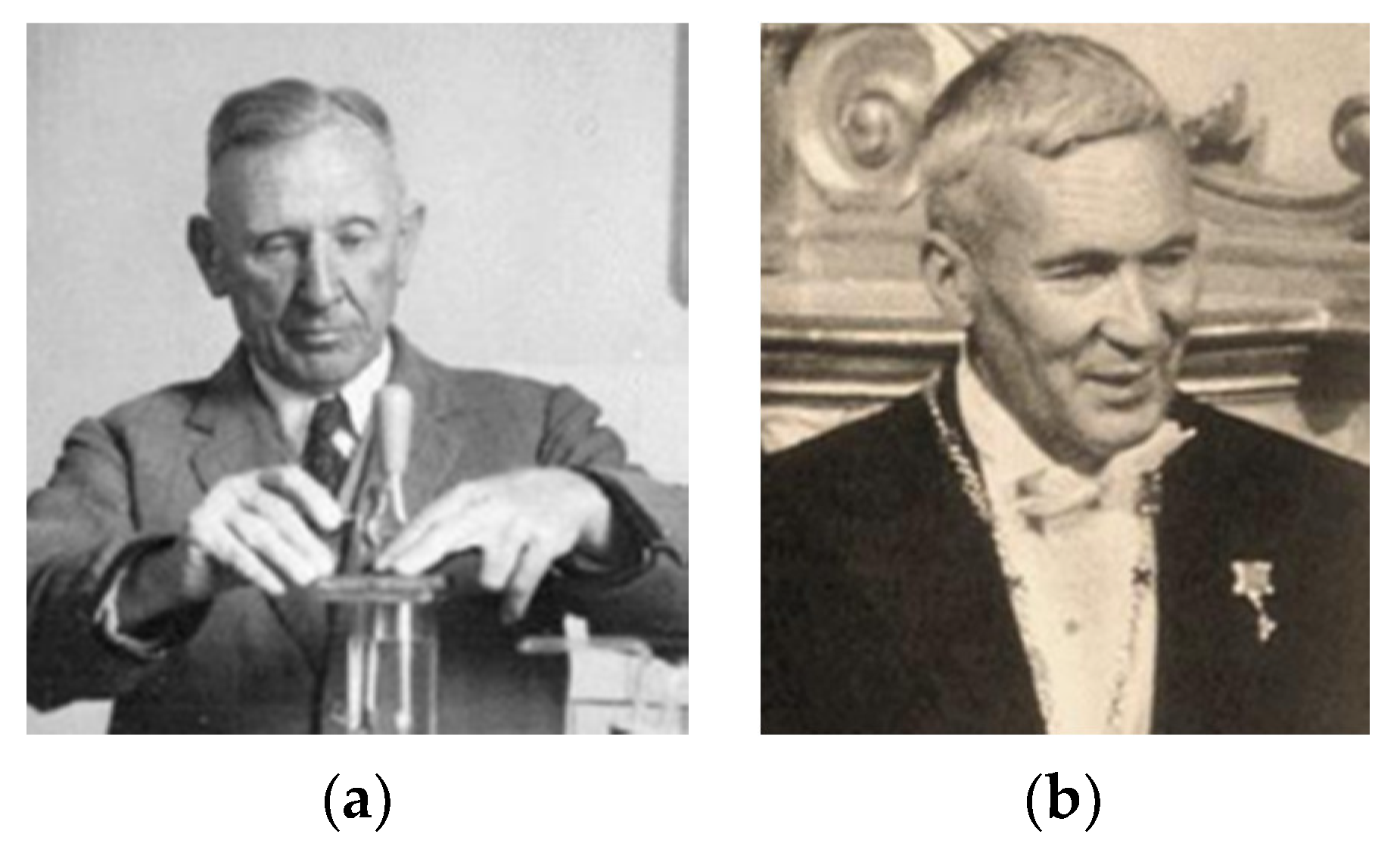
Clustering in nature was first identified by Hurst [1] (Figure 1a) while studying the long-term behavior in a variety of scales of the discharge timeseries of the Nile River to develop engineering projects in its basin. Particularly, Hurst discovered a tendency of high-discharge years to cluster into high-flow periods, and low-discharge years to cluster into low-flow periods. This behavior, also known as the Hurst phenomenon or Joseph effect [2], is characterized by long-term persistence (LTP; also called long-range dependence), which leads to high unpredictability on large scales due to the clustering of events as compared to the purely random process (i.e., white noise) or other short-range dependence models (e.g., Markovian).
The mathematical description of the Hurst phenomenon is attributed to A.N. Kolmogorov (Figure 1b) who developed it while studying turbulence in 1940 [3]. Based on this, Koutsoyiannis [4] coined the term Hurst–Kolmogorov (HK) dynamics (Figure 2), so as to give credit to both contributing scientists and to expand it from the narrower Gaussian LTP processes (e.g., fractional Gaussian noise [5]). The HK dynamics also incorporate short-range dependence (e.g., fractal-type behavior [6]) and intermediate-scale behavior often observed in global-scale hydrological-cycle and turbulent processes [7].
The HK dynamics are also linked to the entropy maximization principle, and thus, to robust physical justification [8]. It is worth noting that the stochastic simulation of the HK dynamics is still a mathematical challenge [9] since it requires the explicit preservation of high-order moments in a vast range of scales [10,11], affecting both the intermittent (fractal) behavior in small scales [12] and the dependence in extremes [13].
The 1D clustering behavior has been identified in many scientific fields (see reviews in [7,15,16,17]). The 2D spatial clustering behavior has also been explored in many fields such as hydrology (e.g., [18,19,20], and references therein), biology and ecosystems (e.g., [21,22]), life sciences (e.g., [23,24,25,26]), networks (e.g., [27,28,29]), urban structures (e.g., [30,31]), rock formation (e.g., [32]), turbulence (e.g., [7,33]), art (e.g., [34,35,36]), landscape analysis (e.g., [37,38]), simulated evolution of the universe [39] and many others (e.g., [40]). A unified approach for the quantification of the 2D spatio-temporal clustering in terms of variability in the scale domain (instead of in the common lag and frequency domains) can be found in the applications of the current entry, where a stochastic methodology is presented that quantifies clustering in 2D spatial fields by analyzing the spatial structures over time, and by exploring how the HK dynamics highly increase the induced uncertainty in terms of spatio-temporal variability in the scale domain.
1.2. Stochastic Analysis in the Scale Domain
The most common stochastic metrics in literature are based on the dependence structure of the second-order statistics (see discussions in [5,7,13,41]), which are commonly estimated through the autocovariance function, c(h), or the autocorrelation function, i.e., c(h)/c(0), where h is the continuous time lag in time units, or through the power spectrum, whose definition is based on c(h), i.e., , where is the continuous frequency in reverse time units. Common estimators of the latter are the so-called periodogram and the autocovariance (or autocorrelation) [42,43]. However, the latter estimators are based only on the domains of lag and frequency. Beran [44], inspired by the empirical work of Smith [45] in agricultural crops and by similar works in other fields [46,47], applied a similar estimator but to the scale domain (i.e., plot in logarithmic axes of the variance of the accumulated or aggregated process vs. scale [48,49]). Nevertheless, this estimator was later abandoned, since it was characterized as a “bad estimator” of the long-term persistence, mainly due to the large estimation bias [43,50]. Another similar estimator for the identification of long-term persistence, introduced by Hurst [1] and known as rescaled range (R/S), was also found to have similar or even worse issues than the aggregated variance method [43,51,52,53,54,55].
The identification of the stochastic structure in the scale domain is revisited much later and compared to the lag domain (i.e., through the correlogram estimator of the autocovariance/autocorrelation function) and the frequency domain (i.e., through the power spectrum), but after theoretically defining the expressions, estimators and bias expressions for all three metrics in the three domains [56].
The aggregated variance was also found to be a misnomer of this method in the scale domain (i.e., the variance is not aggregated but rather the scale is [57]), and a single name for this method did not exist (as, for example, for the periodogram or the correlogram methods); hence, Koutsoyiannis [4] suggested to use the term climacogram to emphasize the graphical representation and the link of the concept to scale (i.e., climax in Greek), and so as not to be confused with the already established term of scale(o)gram. It is noted that the climacogram is explicitly linked to the autocovariance c(h), i.e., , and thus, also to the power spectrum [5].
Through the above works, the climacogram could now be adjusted for estimation bias [10,12,14,56,58,59], as well as the autocovariance and power spectrum for estimation and discretization bias. (See next section for the bias expressions of the multi-dimensional second-order climacogram, while for the autocovariance and power spectrum, the bias expressions can be found in [40,56].) Thus, after eliminating the main criticized limitations of this estimator, Dimitriadis and Koutsoyiannis [56] illustrated how the climacogram outperforms the other two estimators. Particularly, the climacogram is shown (a) to exhibit a smaller estimation bias than the more commonly used tools of autocorrelation and power spectrum (i.e., autocovariance-based metrics); thus, it can robustly identify from fields analysis both the short-term structure and the long-range dependence behavior, with the latter highly linked to the clustering effect, which emerges specifically in complex systems as opposed to the simplest yet uncommon behavior of white noise (absence of dependence) or Markov structure (i.e., short-range dependence); (b) to be free of discretization bias as opposed to the autocovariance-based metrics, in which the transformation of the continuous to discrete representation of the spatio-temporal field is involved due to the double integration calculations; and (c) to be well defined and with a monotonic behavior, as compared to the autocovariance-based metrics, whose double logarithmic slopes (e.g., used to identify the long-term persistence) exhibit a non-monotonic behavior. Thus, a stochastic process with short-term fractal and long-term persistent structures should be analyzed in the scale domain instead of in the lag and frequency domains.
Based on this scientific boost, the climacogram (rather than autocovariance-based metrics) was found preferable for the identification, model building and simulation of a stochastic process. Since then, the interest in the scale domain has been highly increased, and the climacogram has been used to identify the LTP behavior in various scientific studies. For a review of such studies, see [7,13] and references therein, where also a massive global-scale analysis in the scale domain is included for several hydrological-cycle processes (i.e., near-surface air temperature, dew point, humidity, atmospheric pressure, near-surface wind speed, streamflow and precipitation) and microscale turbulent processes (such as grid turbulence and turbulent jets). Alternative scientific fields, where the analysis is performed in the scale domain and by using the climacogram, include studies of rock formations [32], landscapes [37,38], water–energy nexus [60,61], time-irreversible processes [62,63], multilayer perceptron [64] and many others [65] as shown in the applications of the entry. It is again emphasized that this entry focuses on the multi-dimensional spatio-temporal stochastic metrics in the scale domain, as presented in the next sections.
2. Methodology
For the exploration of change and estimation of the spatio-temporal variability in the scale domain (instead of in the traditional lag and frequency domains), we use the stochastic metric of the climacogram, as thoroughly discussed in the previous section.
Particularly, we expand the 1D scale domain to an -dimensional (D) one. We denote , the continuous-state random variable of a stochastic stationary and isotropic process in L dimensions, with , a vector of variables, and , an index varying from 1 to , i.e., , that is used to describe each dimension of the process (e.g., can be a temporal variable, a spatial one etc.). Note that the L dimensions are considered independent of each other. Discretized processes are subject to a sampling frequency and a response time as in the 1D case. Both and have the same units with the corresponding variable (e.g., if is a temporal variable measured in seconds then and will be measured also in seconds). Here, we focus only on the case of = > 0. Finally, n denotes the total amount of data in the D field. Thus, the discretized stochastic process , for > 0, can be estimated from the continuous stochastic process as [40]:
where are indices of each variable in .
In Table 1, we provide all necessary definitions and equations for the true continuous, true discrete and most common estimators and estimations for the expected climacogram for a D process (for the autocovariance, variogram and power spectrum, see [40]). As shown in Table 1, the climacogram estimator is expressed through the classical estimator of variance, but other and higher-order moments can be used (e.g., [13]).
For example, the second-order climacogram estimator in two dimensions (i.e., called 2D-C) is shown for the estimation of spatial variance vs. scale, where the spatial scale is defined as the ratio of the area of k × k adjacent cells (i.e., scale k), whose values are averaged to form the (scaled) spatial field. The 2D-C is defined as (see also [13]):
where the ‘^’ over γ denotes estimate, κ is the dimensionless spatial scale, represents the local average of the space-averaged process at scale κ and at grid cell (i, j) and upper-lined x is the global average, while underlined variables represent random variables as opposed to regular ones. Note that Δ = 1 and the maximum available scale for this estimator is n/2, but estimation beyond n/10 is not reliable [56].
As previously mentioned, an important stochastic process that characterizes the variability over small and large scales is the Hurst–Kolmogorov (HK) behavior. For example, the general case of an LD HK process can be described by the equation:
where μ is the mean of the process , and is the same process at scale κ.
The D climacogram in the continuous-scale domain can be expressed as:
where is now the geometric mean of scales , ,…, , i.e., , α is a scale parameter in units of , so that , and H is the Hurst parameter (0 < H < 1). For 0 < H < 0.5, the HK process exhibits an anti-persistent behavior, while H = 0.5 corresponds to the white noise process, and for 0.5 < H < 1, the process exhibits persistence, a common behavior exhibited in nature.
The long-term persistence behavior can be quantified by the Hurst parameter as described by the previous equation. The problem with this process is that it yields an infinite variance as scale tends to zero. One way to remedy this is by introducing a modified and also generalized form of the HK model, which was found to be efficient in geophysical processes [7], and as also shown in the applications, as it can simulate both short-term and long-term dependence structures. This can be expressed in a standardized form through the climacogram expression (for additional models, see [7,13]) as:
where 0 < M < 1 is a fractal parameter indicative of the roughness of the process. For M < 0.5, the process is characterized as rough, and M > 0.5 as smooth, whereas for M = 0.5, there is neutrality, corresponding to the so-called generalized (GHK) model [6].
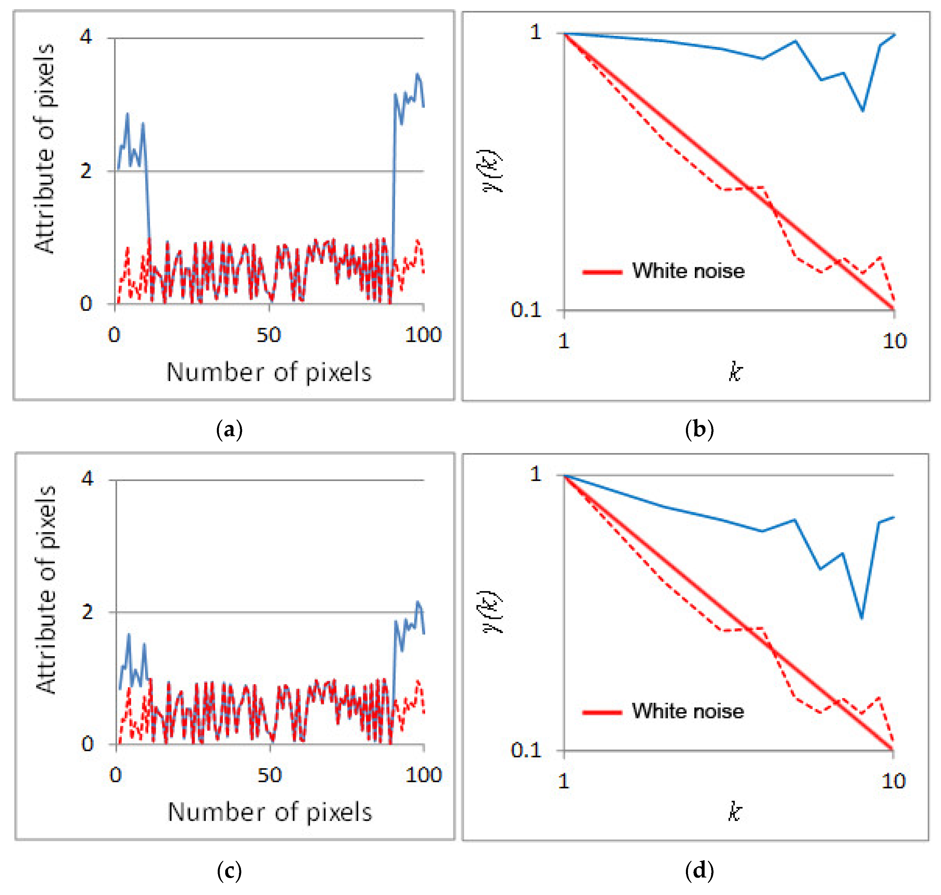
Finally, since the clustering behavior is of particular interest for this entry, we show a simple example of how a cluster in a timeseries can be easily identified through the second-order climacogram (i.e., plot of variance of the averaged process vs. scale in logarithmic axes). In Figure 3a,c, the cases of two 1D data series are depicted, each with a different change in magnitude at the beginning and at the end of the series. The data series with the larger change in magnitude Figure 3a corresponds to the climacogram with the higher log-log slope (Figure 3b), which is an indication of a stronger clustering behavior of the 1D data series. Similarly, the weaker clustering behavior, although still stronger than in the white noise one, corresponds to the smaller log-log slope of the climacogram (Figure 3d) and the data series with the smaller change in magnitude (Figure 3a).
3. Illustrative Applications
3.1. One-Dimensional Turbulence
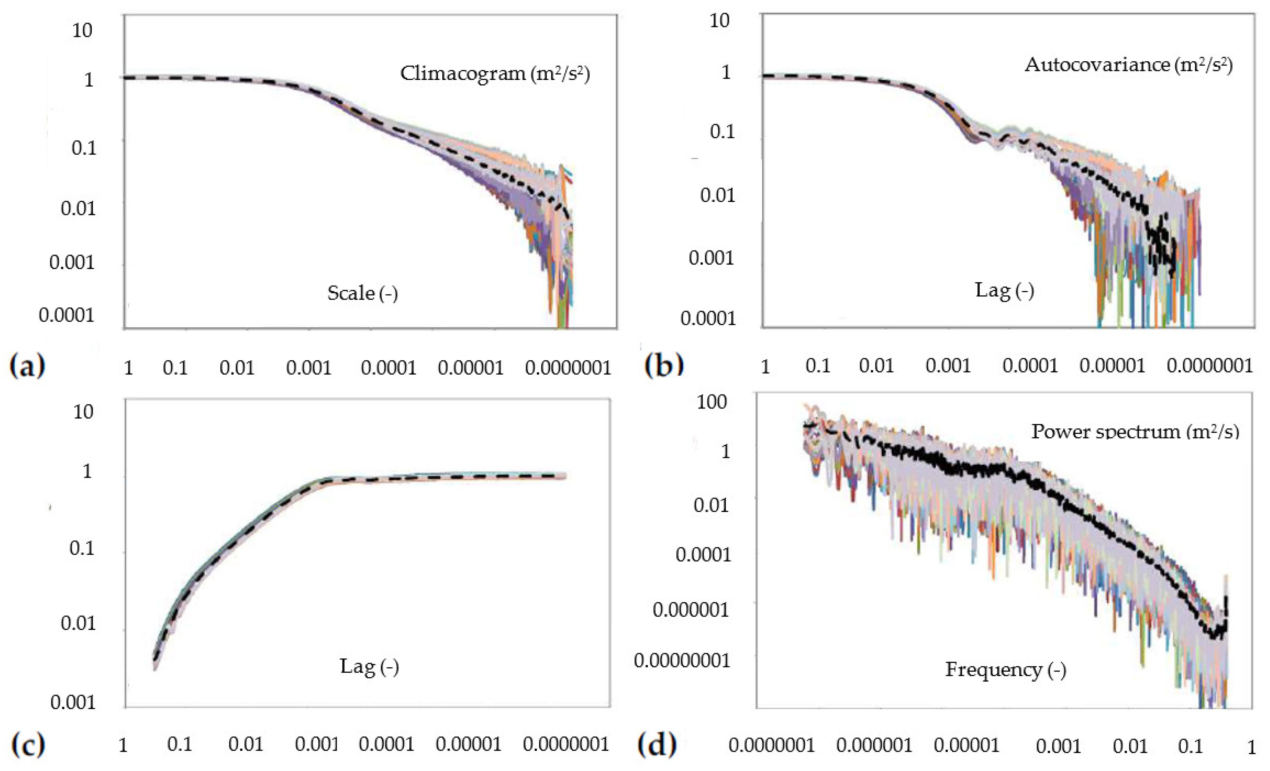
Here, we present the analysis of a massive dataset comprising 40 timeseries of the longitudinal velocity behind a grid provided by the John Hopkins university [66]. Each timeseries comprises 36 × 106 records, and after a data-homogenization procedure, we were able to analyze them as if they were recorded at the same location and with similar initial conditions (for more details on the homogenization, see [12]). In Figure 4, we show the standardized second-order metrics of the climacogram, autocovariance and variogram, i.e., c(h) − c(0), and power spectrum, where it can be seen that the variogram and the climacogram exhibit the smallest uncertainty at the long-range scales and, in particular, on the double logarithmic slope that is attributed to the strength of the long-range dependence (i.e., the magnitude of the Hurst parameter). However, since the variogram has the limitation that the double logarithmic slope tends to zero, only from the climacogram is it possible to robustly estimate the Hurst parameter (for comparison between the two metrics, see [32]).
3.2. Benchmark Analysis of Two-Dimensional Art Paintings
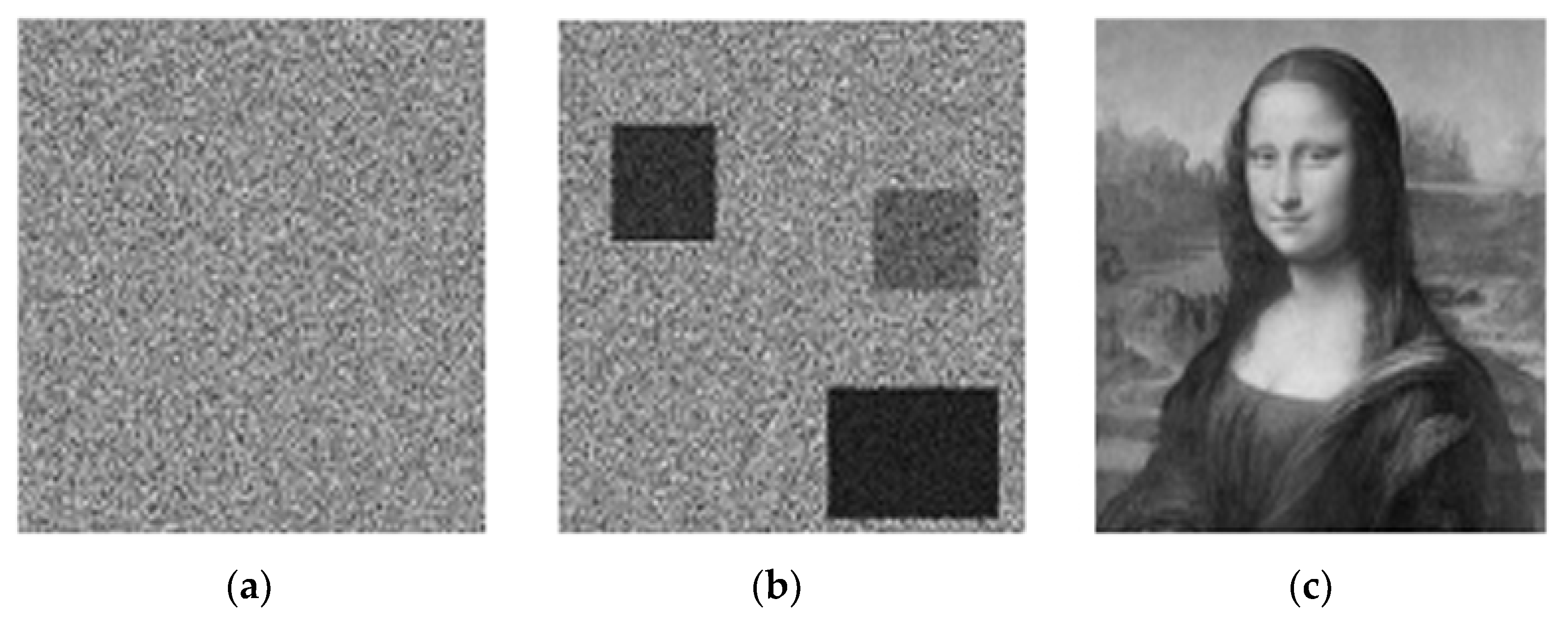
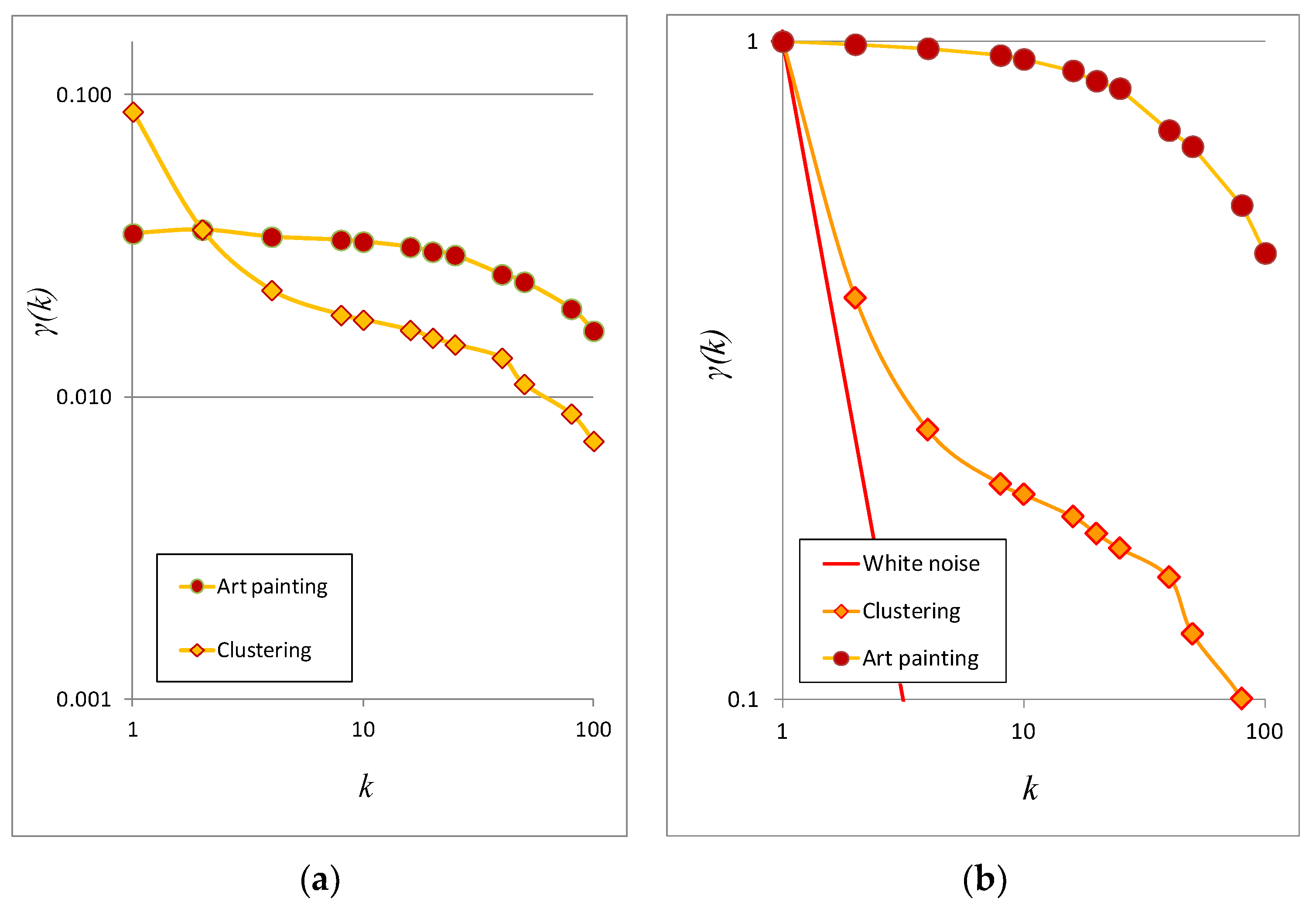
Here, we show an application of the stochastic metric 2D-C in a benchmark white noise process without (Figure 5a) and with (Figure 5b) cluster areas, and we compare this to a famous art painting (Figure 5c). Particularly, in Figure 6, we show how the 2D-C can effectively be used for comparison of the magnitude of the variabilities among images. Specifically, it illustrates how much larger and smaller is the variability vs. the scale of the benchmark image when including a few cluster areas, as compared to that of the white noise process and to that of the art painting, respectively.
3.3. Two-Dimensional Rock-Formations
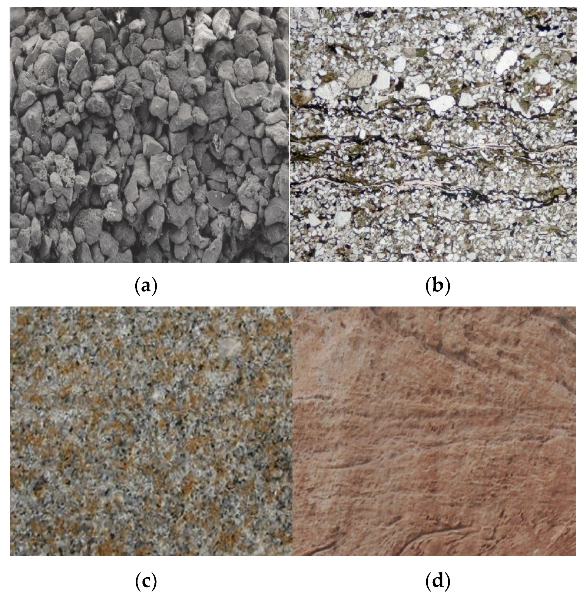
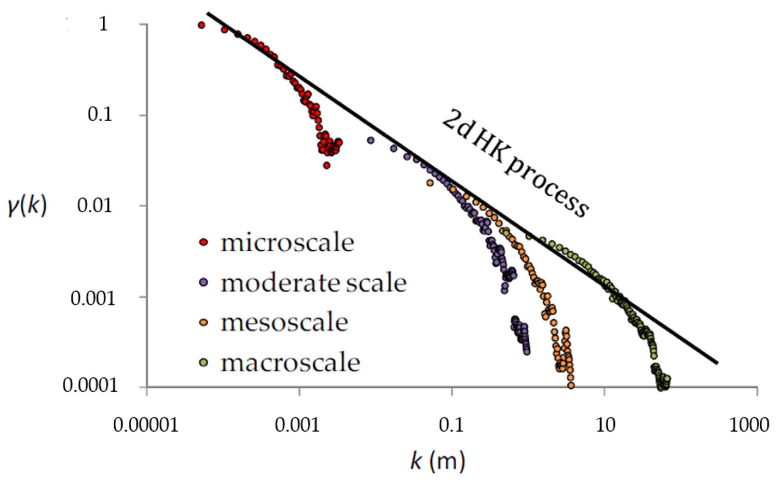
Here, we show the application of the 2D-C metric at images of sandstones depicted at different spatial scales of 8 orders of magnitude (Figure 7 and Figure 8). We see how all the different samples can be both easily compared to each other, in terms of the variability, and unified under the HK dynamics, when analyzed through the scale domain (for more information on the samples and the derived Hurst parameter, see [32]).
3.4. Spatio-Temporal Wind Speed of a Hurricane
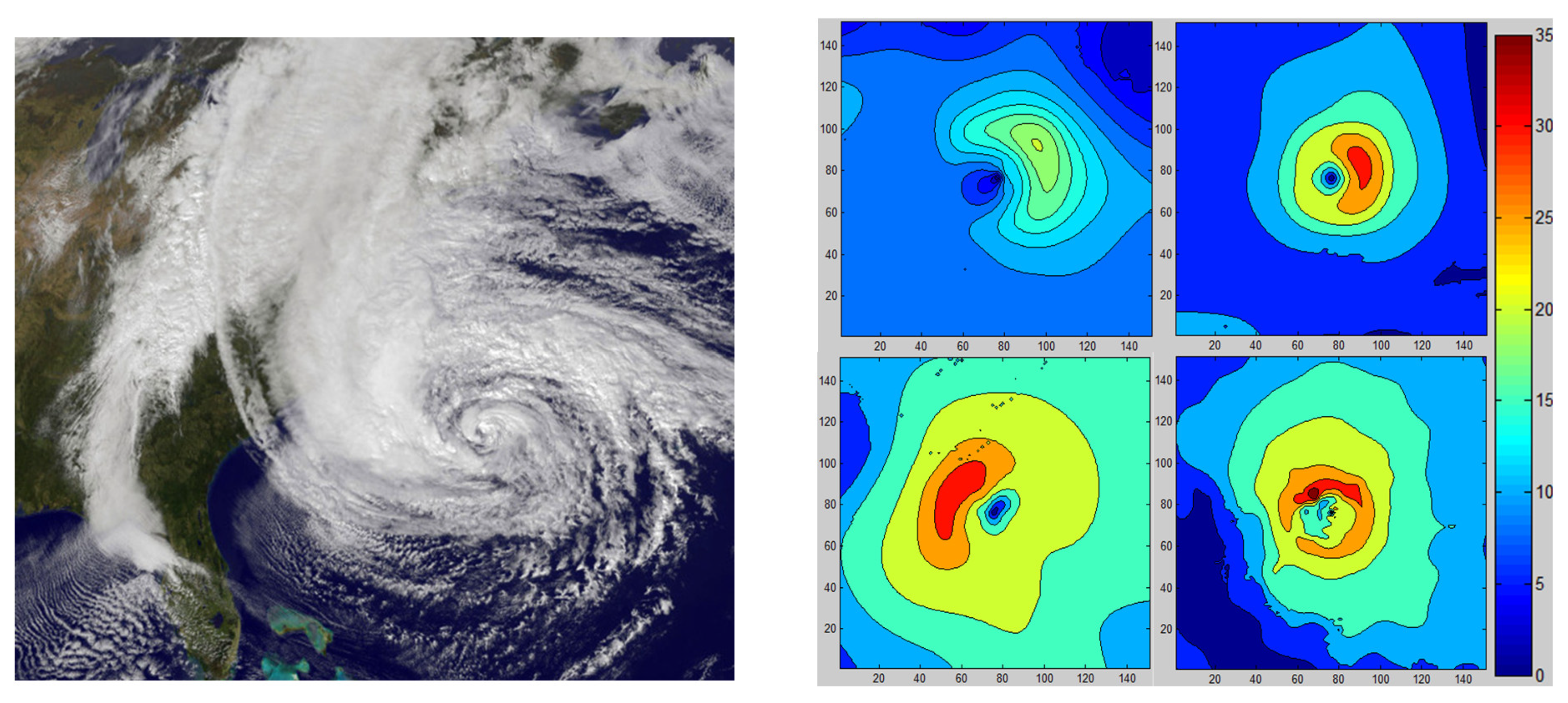
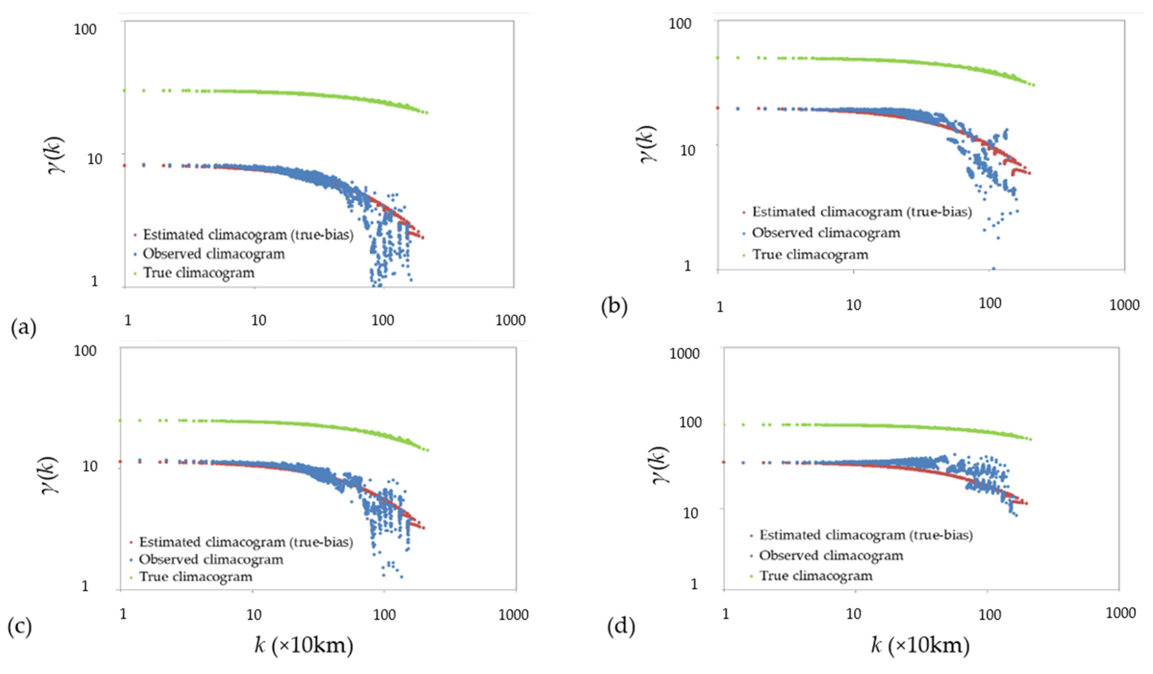
Next, we apply the 2D-C metric to a spatial image of wind speed magnitude from Hurricane Sandy (www.nhc.noaa.gov/data), observed in October 2012 (Figure 9). As the starting point for the estimation of the climacogram, we chose the center of the image, which has approximately 0 wind speed as it is the eye of the hurricane [40]. In Figure 10, we estimate the climacogram of the hurricane images in several time frames (observed climacogram), and we fit, for illustration, the GHK model (denoted as true climacogram) by adjusting for bias (that is extremely high in this example), a procedure that is usually neglected in stochastic analysis.
3.5. Spatio-Temporal Evolution of Clustering
The tool called 2D-C quantifies the variability of images through the variance of the brightness intensity in grayscale. By a careful selection of images with spatial information, we can quantify how clustering alters over time, which can be useful for either characterizing spatial variability, such as in urbanization, and thus enabling tracking of their spatio-temporal evolution, or for revealing spatial hidden patterns through scales that may be invisible in the first glance of the image. A range of such applications is presented in [39], with focus in (a) natural sciences, in terms of the evolution of the universe as suggested by cosmological simulations and of the ecosystems, such as forests and lakes, and in (b) social sciences dealing with social structures, as revealed by the evolution of worldwide cropland data, satellite images of night lights and spatial data on urban land cover.
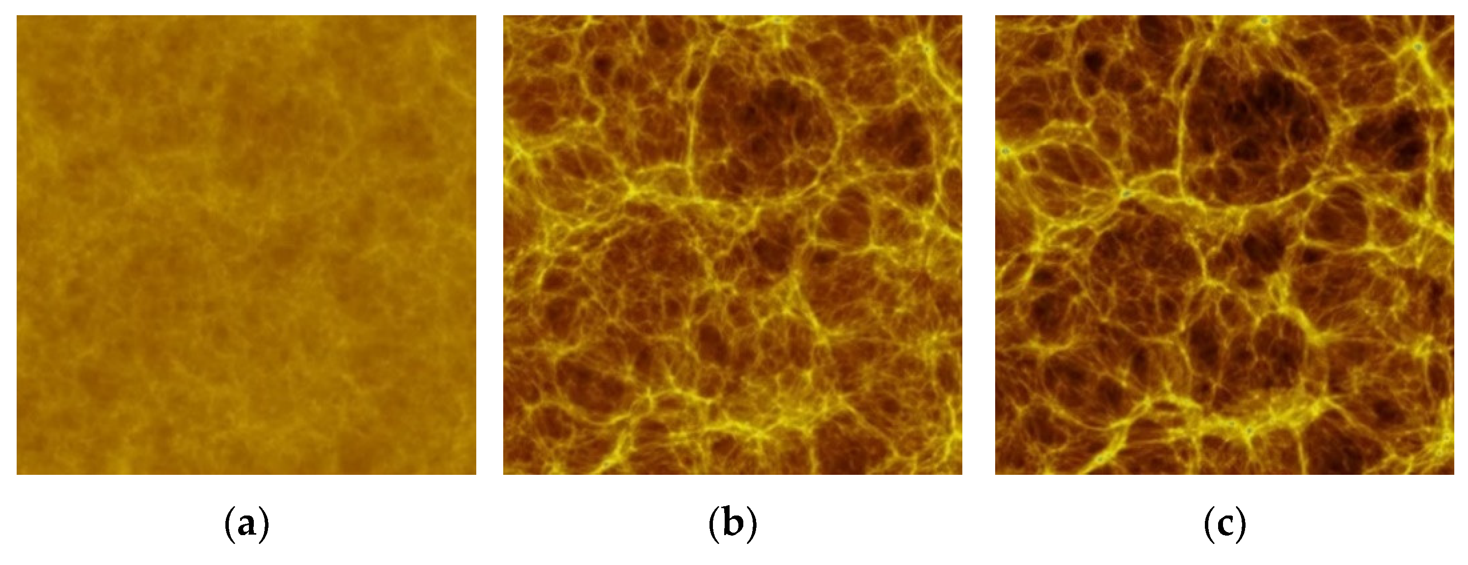
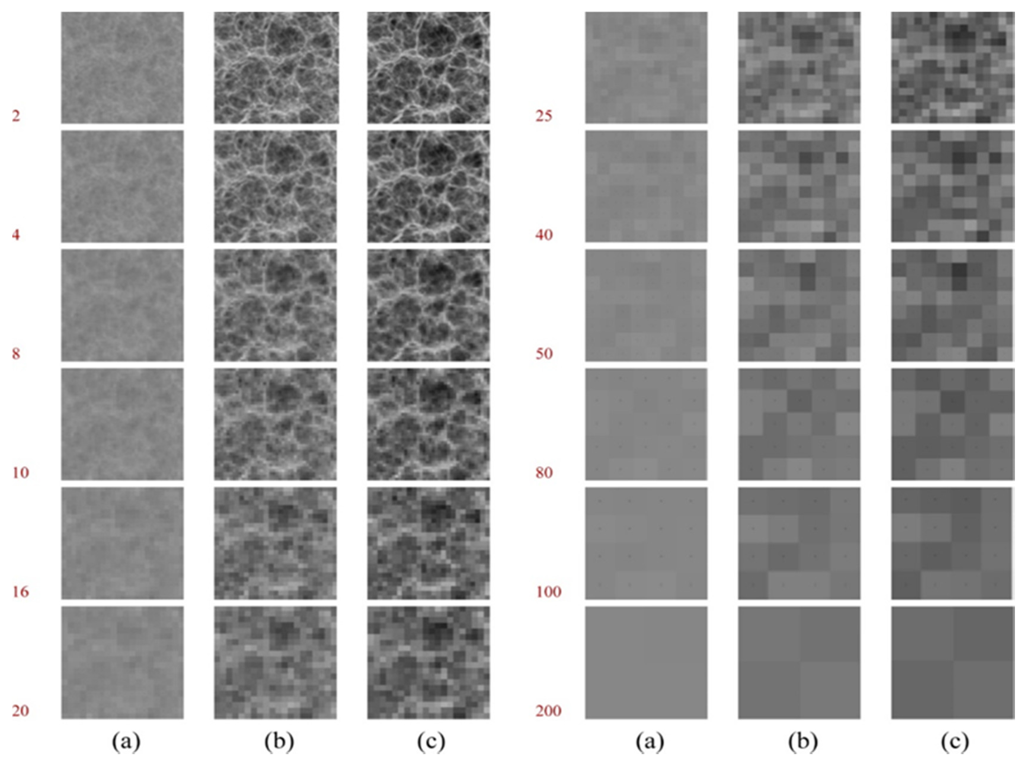
Here, the 2D-C is implemented for the estimation of spatial variance vs. scale in temporal sequence of images (after being processed by filtering or enhancing techniques [65]). The pixels analyzed are represented by numbers denoting their color intensity in grayscale (white = 1, black = 0). Figure 11 presents images from three timeframes of the evolution of the universe as generated by a cosmological model of evolution [67]: (a) 500 million years after Big Bang, an image with faint clustering; (b) 1000 million years after Big Bang, an image with mild clustering; and (c) 10,000 million years after Big Bang, an image with intense clustering. Figure 12 depicts the scaled images at scales k = 2, 4, 8, 16, 20, 25, 40, 50, 80, 100 and 200, which are used to calculate the 2D climacogram.
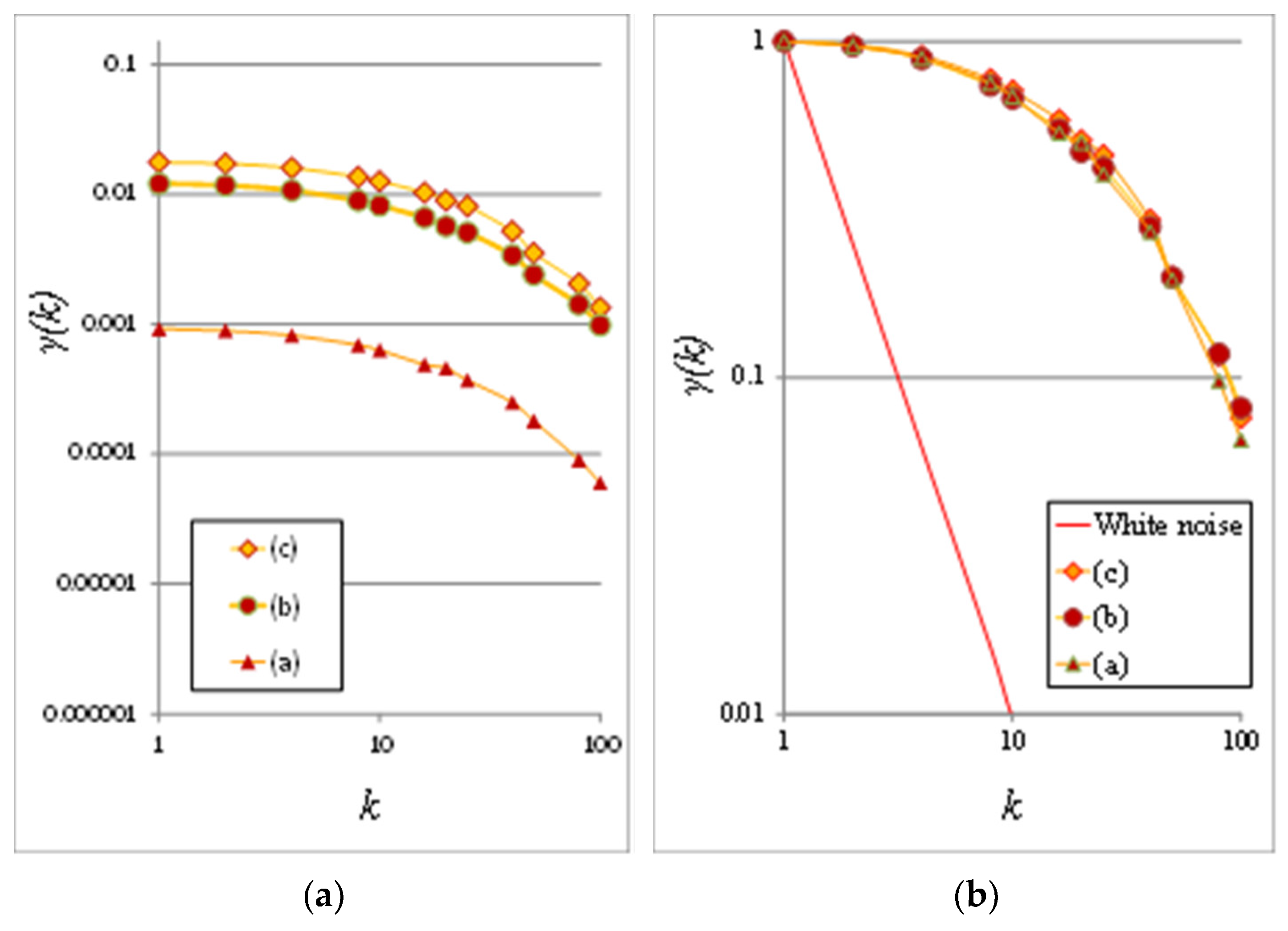
The presence of clustering is reflected in the climacogram (Figure 13a,b), which shows a marked difference as the scale increases. Specifically, the variance of the images is notably higher at the scales with higher clustering, indicating a greater degree of variability of the process at these scales.
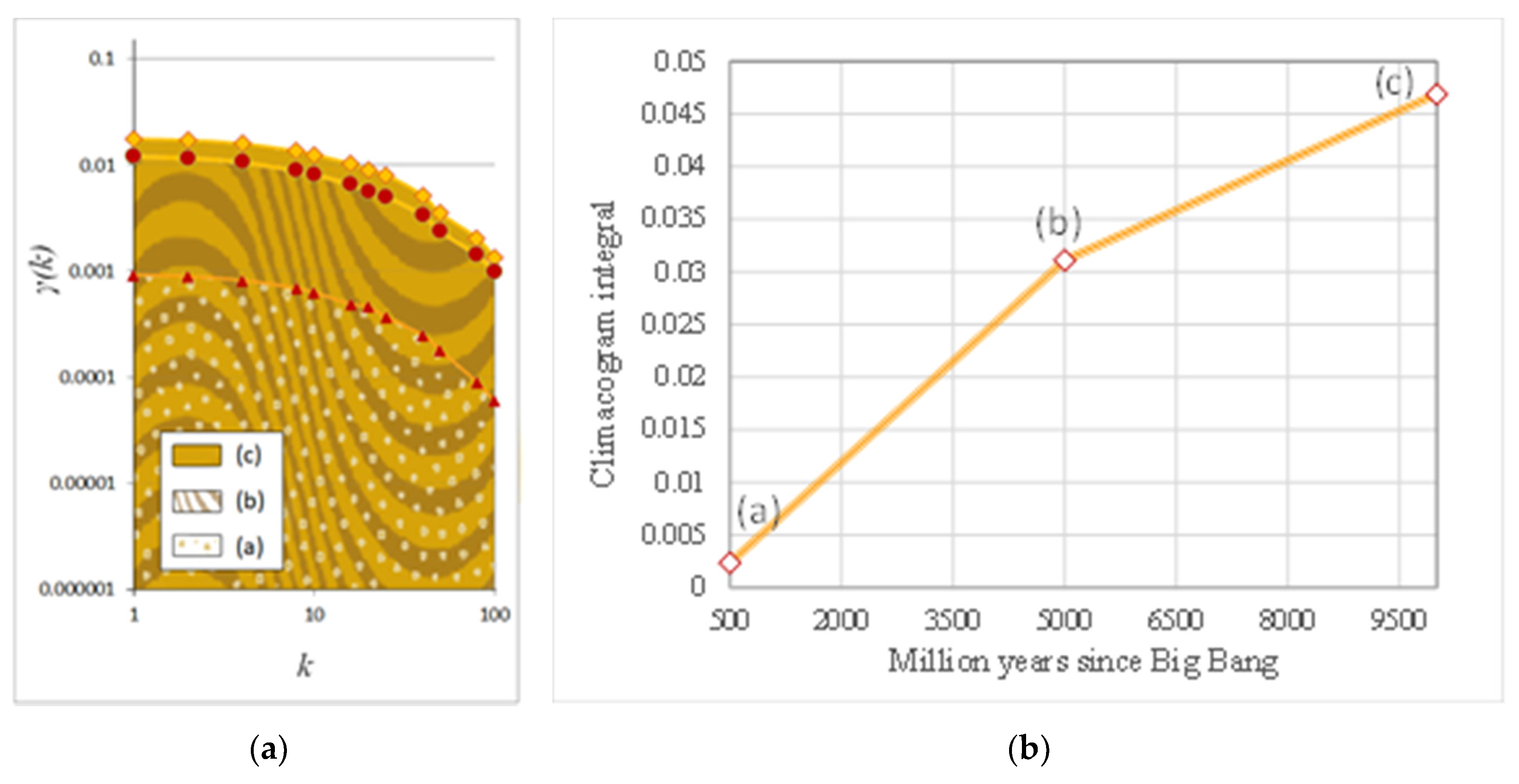
For the integration of all information contained in the 2D climacogram of each image, we evaluate the cumulative areas underneath each one for all scales, i.e., the climacogram integral , where Δ and k are the minimum and maximum scale, and we divided by x in order for the integral to converge for arbitrarily high k (). In the discrete case, this can be approximated as:
where n(k) is the number of integration intervals for scale k. We evaluate at the maximum available spatial scale, so that it is the best approximation of the limit .
In Figure 14a,b, each climacogram is represented by its corresponding integral, permitting the evaluation of the rate of the alteration of clustering through time.
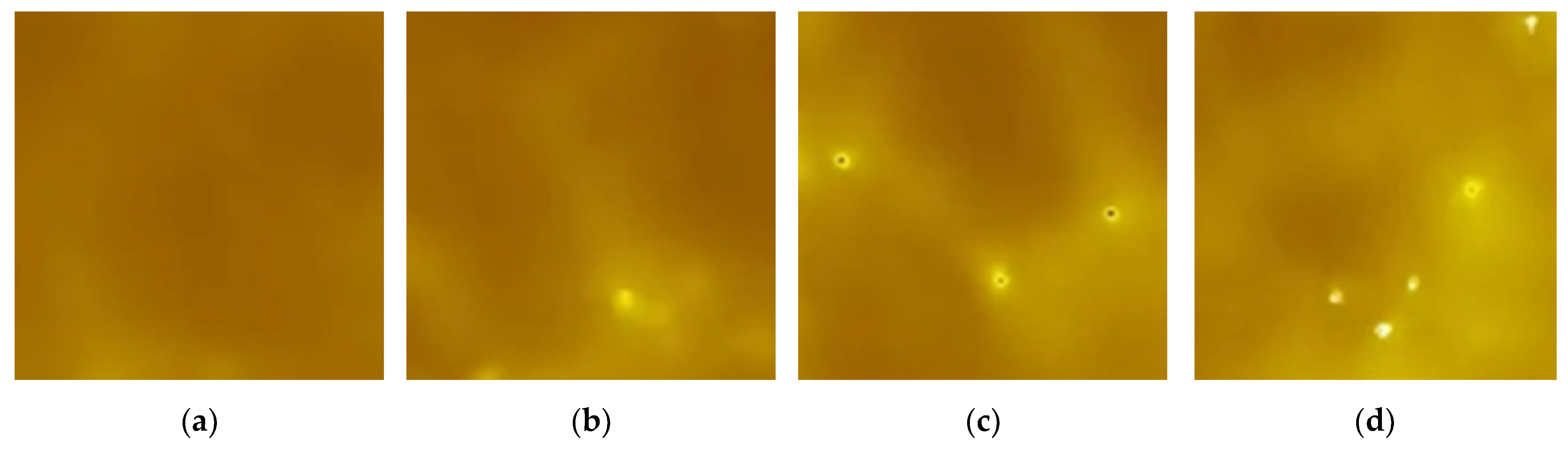
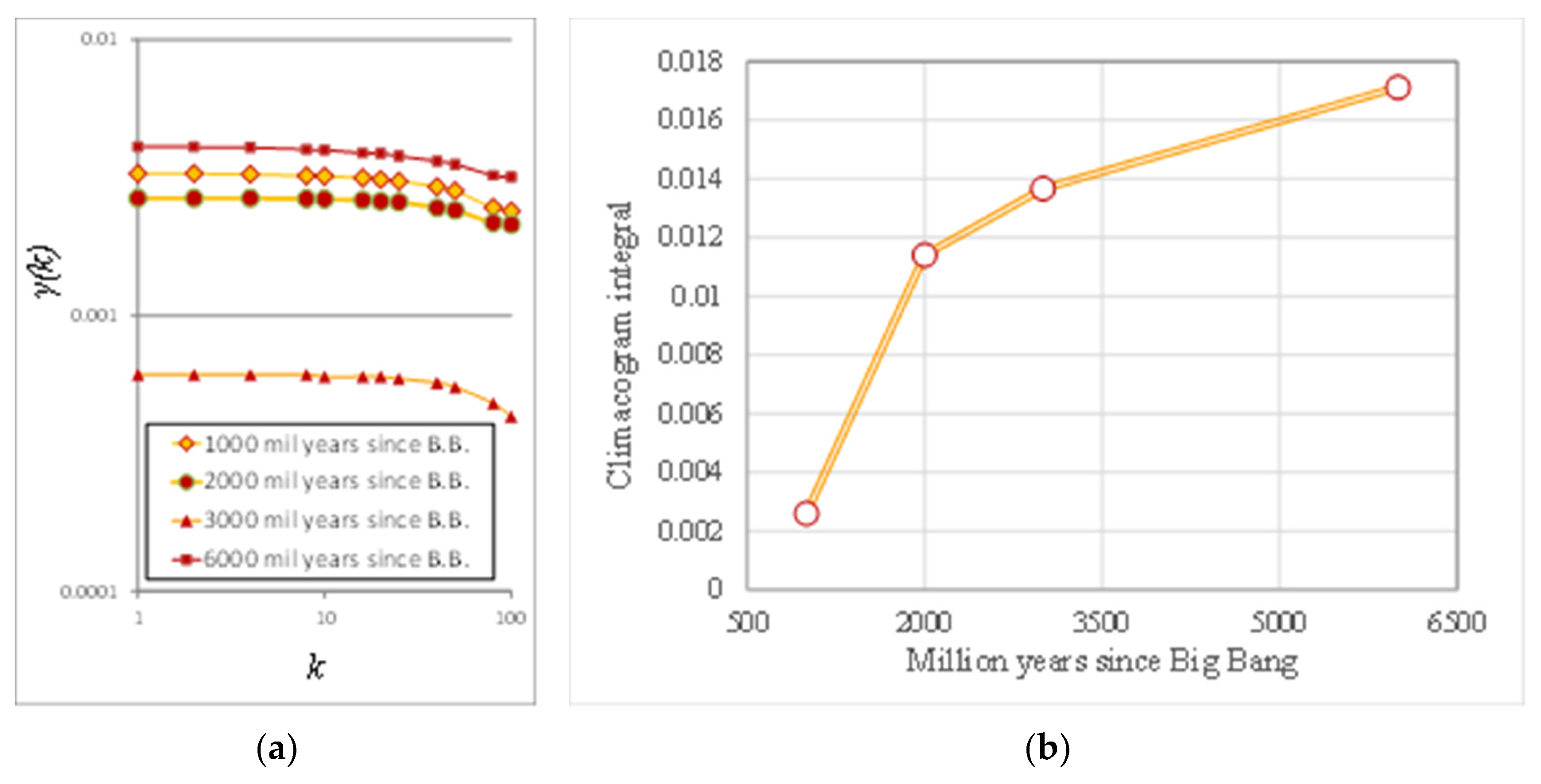
One more example is given in Figure 15 and Figure 16, where we evaluate the evolution of clustering in (randomly picked) zoomed areas from the original images of the evolution of the universe of clustering through time.
This method enables the comparison of clustering patterns at various spatial scales and among different time frames, and it is a meaningful metric for understanding and quantifying the change in clustering through time.
4. Conclusions
The Hurst–Kolmogorov dynamics describe a commonly observed structure in multidimensional spatio-temporal natural processes, which includes a short-term (fractal) structure in small scales and a long-range dependence (or persistence) behavior in large ones. The latter attribute is linked to the clustering effect of a spatio-temporal stationary stochastic process with an arbitrary marginal distribution function and a power-type dependence structure in large spatio-temporal scales yielding a high probability of low- (or high-) magnitude events to group together in space and time.
The analysis in the scale domain through the climacogram (instead of in the common lag and frequency domains, through the autocovariance and power spectrum, respectively) can effectively be used for identification and simulation of the Hurst–Kolmogorov behavior in a vast range of scales. Moreover, through spatio-temporal information, we can quantify how clustering alters over time, which can be useful for either characterizing spatial variability, thus enabling tracking of their spatio-temporal evolution, or for revealing hidden patterns through scales that may be difficult to trace with conventional methods.
The exploration of different topics in the stochastic nature of natural processes on a multidimensional spatio-temporal scale domain can be numerous and related to different scientific fields, as illustrated in the literature review and the presented applications of the current entry.
Author Contributions
Conceptualization, P.D., T.I., G.-F.S. and D.K.; methodology, P.D., T.I., G.-F.S. and D.K.; validation, P.D., T.I., G.-F.S. and D.K.; writing—original draft preparation, P.D., T.I., G.-F.S. and D.K.; writing—review and editing, P.D., T.I., G.-F.S. and D.K. All authors have read and agreed to the published version of the manuscript.
Funding
This research received no external funding.
Institutional Review Board Statement
Not applicable.
Conflicts of Interest
The authors declare no conflict of interest.
Entry Link on the Encyclopedia Platform
References
- Hurst, H.E. Long term storage capacities of reservoirs. Trans. Am. Soc. Civ. Eng. 1951, 116, 770–799. [Google Scholar] [CrossRef]
- Mandelbrot, B.B.; Wallis, J.R. Noah, Joseph and operational hydrology. Water Resour. Res. 1968, 4, 909–918. [Google Scholar] [CrossRef]
- Kolmogorov, A.N. Wiener spirals and some other interesting curves in a Hilbert space. In Selected Works of A. N. Kolmogorov; Mathematics and Mechanics; Tikhomirov, V.M., Ed.; Kluwer: Dordrecht, The Netherlands, 1991; pp. 303–307. [Google Scholar]
- Koutsoyiannis, D. A random walk on water. Hydrol. Earth Syst. Sci. 2010, 14, 585–601. [Google Scholar] [CrossRef]
- Papoulis, A.; Pillai, S.U. Stochastic Processes; McGraw-Hill: New York, NY, USA, 1991. [Google Scholar]
- Gneiting, T.; Schlather, M. Stochastic Models That Separate Fractal Dimension and the Hurst Effect. SIAM Rev. 2004, 46, 269–282. [Google Scholar] [CrossRef]
- Dimitriadis, P.; Koutsoyiannis, D.; Iliopoulou, T.; Papanicolaou, P. A Global-Scale Investigation of Stochastic Similarities in Marginal Distribution and Dependence Structure of Key Hydrological-Cycle Processes. Hydrology 2021, 8, 59. [Google Scholar] [CrossRef]
- Koutsoyiannis, D. Hurst–Kolmogorov dynamics as a result of extremal entropy production. Phys. A Stat. Mech. Appl. 2011, 390, 1424–1432. [Google Scholar] [CrossRef]
- Koutsoyiannis, D.; Dimitriadis, P. Towards generic simulation for demanding stochastic processes. Science 2021, 3, 34. [Google Scholar] [CrossRef]
- Koutsoyiannis, D. Generic and parsimonious stochastic modelling for hydrology and beyond. Hydrol. Sci. J. 2016, 61, 225–244. [Google Scholar] [CrossRef]
- Beven, K. Issues in Generating Stochastic Observables for Hydrological Models. Hydrol. Process. 2021. [Google Scholar] [CrossRef]
- Dimitriadis, P.; Koutsoyiannis, D. Stochastic synthesis approximating any process dependence and distribution. Stoch. Environ. Res. Risk Assess. 2018, 32, 1493–1515. [Google Scholar] [CrossRef]
- Koutsoyiannis, D. Stochastics of Hydroclimatic Extremes—A Cool Look at Risk; Edition 0; National Technical University of Athens: Athens, Greece, 2021; 330p. [Google Scholar]
- Koutsoyiannis, D. Hurst-Kolmogorov Dynamics and Uncertainty. J. Am. Water Resour. Assoc. 2011, 47, 481–495. [Google Scholar] [CrossRef]
- Beran, J.; Feng, Y.; Ghosh, S.; Kulik, R. Long-Memory Processes; Springer: Berlin/Heidelberg, Germany, 2013. [Google Scholar] [CrossRef]
- O’Connell, P.; Koutsoyiannis, D.; Lins, H.F.; Markonis, Y.; Montanari, A.; Cohn, T. The scientific legacy of Harold Edwin Hurst (1880–1978). Hydrol. Sci. J. 2016, 61, 1571–1590. [Google Scholar] [CrossRef]
- Graves, T.; Gramacy, R.; Watkins, N.; Franzke, C. A Brief History of Long Memory: Hurst, Mandelbrot and the Road to ARFIMA, 1951–1980. Entropy 2017, 19, 437. [Google Scholar] [CrossRef]
- Koutsoyiannis, D.; Paschalis, A.; Theodoratos, N. Two-dimensional Hurst–Kolmogorov process and its application to rainfall fields. J. Hydrol. 2011, 398, 91–100. [Google Scholar] [CrossRef]
- Paschalis, A.; Molnar, P.; Fatichi, S.; Burlando, P. A stochastic model for high-resolution space-time precipitation simulation. Water Resour. Res. 2013, 49, 8400–8417. [Google Scholar] [CrossRef]
- Varouchakis, E.A.; Hristopulos, D.T. Comparison of spatiotemporal variogram functions based on a sparse dataset of ground-water level variations. Spat. Stat. 2017, 34, 100245. [Google Scholar] [CrossRef]
- McGarvey, R.; Feenstra, J.E.; Mayfield, S.; Sautter, E.V. A diver survey method to quantify the clustering of sedentary invertebrates by the scale of spatial autocorrelation. Mar. Freshw. Res. 2010, 61, 153–162. [Google Scholar] [CrossRef]
- Tachmazidou, I.; Verzilli, C.J.; De Iorio, M. Genetic Association Mapping via Evolution-Based Clustering of Haplotypes. PLoS Genet. 2007, 3, e111. [Google Scholar] [CrossRef]
- Hütt, M.-T.; Neff, R. Quantification of spatiotemporal phenomena by means of cellular automata techniques. Phys. A Stat. Mech. Appl. 2001, 289, 498–516. [Google Scholar] [CrossRef]
- Khater, I.M.; Nabi, I.R.; Hamarneh, G. A Review of Super-Resolution Single-Molecule Localization Microscopy Cluster Analysis and Quantification Methods. Patterns 2020, 1, 100038. [Google Scholar] [CrossRef]
- Murase, K.; Kikuchi, K.; Miki, H.; Shimizu, T.; Ikezoe, J. Determination of arterial input function using fuzzy clustering for quantification of cerebral blood flow with dynamic susceptibility contrast-enhanced MR imaging. J. Magn. Reson. Imaging 2001, 13, 797–806. [Google Scholar] [CrossRef]
- Mier, P.; Andrade-Navarro, M.A. FastaHerder2: Four Ways to Research Protein Function and Evolution with Clustering and Clustered Databases. J. Comput. Biol. 2016, 23, 270–278. [Google Scholar] [CrossRef] [PubMed]
- McDermott, P.L.; Wikle, C.K. Bayesian Recurrent Neural Network Models for Forecasting and Quantifying Uncertainty in Spatial-Temporal Data. Entropy 2019, 21, 184. [Google Scholar] [CrossRef]
- Papacharalampous, G.; Tyralis, H.; Koutsoyiannis, D. Comparison of stochastic and machine learning methods for multi-step ahead forecasting of hydrological processes. Stoch. Environ. Res. Risk Assess. 2019, 33, 481–514. [Google Scholar] [CrossRef]
- Abe, S.; Suzuki, N. Dynamical evolution of clustering in complex network of earthquakes. Eur. Phys. J. B 2007, 59, 93–97. [Google Scholar] [CrossRef]
- Ellam, L.; Girolami, M.; Pavliotis, G.A.; Wilson, A. Stochastic modelling of urban structure. Proc. R. Soc. A Math. Phys. Eng. Sci. 2018, 474, 20170700. [Google Scholar] [CrossRef]
- Levine, N. Spatial Statistics and GIS: Software Tools to Quantify Spatial Patterns. J. Am. Plan. Assoc. 1996, 62, 381–391. [Google Scholar] [CrossRef]
- Dimitriadis, P.; Tzouka, K.; Koutsoyiannis, D.; Tyralis, H.; Kalamioti, A.; Lerias, E.; Voudouris, P. Stochastic investigation of long-term persistence in two-dimensional images of rocks. Spat. Stat. 2019, 29, 177–191. [Google Scholar] [CrossRef]
- Pandey, P.; Mitra, D. Clustering and energy spectra in two-dimensional dusty gas turbulence. Phys. Rev. E 2019, 100, 013114. [Google Scholar] [CrossRef]
- Sargentis, G.F.; Ioannidis, R.; Chiotinis, M.; Dimitriadis, P.; Koutsoyiannis, D. Aesthetical Issues with Stochastic Evaluation. In Data Analytics for Cultural Heritage; Belhi, A., Bouras, A., Al-Ali, A.K., Sadka, A.H., Eds.; Springer: Cham, Switzerland, 2021. [Google Scholar] [CrossRef]
- Sargentis, G.-F.; Dimitriadis, P.; Koutsoyiannis, D. Aesthetical Issues of Leonardo Da Vinci’s and Pablo Picasso’s Paintings with Stochastic Evaluation. Heritage 2020, 3, 283–305. [Google Scholar] [CrossRef]
- Sargentis, G.-F.; Dimitriadis, P.; Iliopoulou, T.; Koutsoyiannis, D. A Stochastic View of Varying Styles in Art Paintings. Heritage 2021, 4, 21. [Google Scholar] [CrossRef]
- Sargentis, G.-F.; Dimitriadis, P.; Ioannidis, R.; Iliopoulou, T.; Koutsoyiannis, D. Stochastic Evaluation of Landscapes Transformed by Renewable Energy Installations and Civil Works. Energies 2019, 12, 2817. [Google Scholar] [CrossRef]
- Sargentis, G.-F.; Ioannidis, R.; Iliopoulou, T.; Dimitriadis, P.; Koutsoyiannis, D. Landscape Planning of Infrastructure through Focus Points’ Clustering Analysis. Case Study: Plastiras Artificial Lake (Greece). Infrastructures 2021, 6, 12. [Google Scholar] [CrossRef]
- Sargentis, G.-F.; Iliopoulou, T.; Sigourou, S.; Dimitriadis, P.; Koutsoyiannis, D. Evolution of clustering quantified by a stochastic method—Case studies on natural and human social structures. Sustainability 2020, 12, 7972. [Google Scholar] [CrossRef]
- Dimitriadis, P.; Koutsoyiannis, D.; Onof, C. N-Dimensional generalized Hurst-Kolmogorov process and its application to wind fields. In Proceedings of the Facets of Uncertainty: 5th EGU Leonardo Conference—Hydrofractals 2013—STAHY 2013, Kos Island, Greece, 17–19 October 2013. [Google Scholar] [CrossRef]
- Lombardo, F.C.; Volpi, E.; Koutsoyiannis, D.; Papalexiou, S.M. Just two moments! A cautionary note against use of high-order moments in multifractal models in hydrology. Hydrol. Earth Syst. Sci. 2014, 18, 243–255. [Google Scholar] [CrossRef]
- Geweke, J.; Porter-Hudak, S. The estimation and application of long memory time series models. J. Time Ser. Anal. 1983, 4, 221–238. [Google Scholar] [CrossRef]
- Beran, J. Statistical Methods for Data with Long-Range Dependence. Stat. Sci. 1992, 7, 404–416. [Google Scholar]
- Beran, J. Estimation, Testing and Prediction for Self-Similar and Related Processes. Ph.D. Thesis, ETH Zurich, Zurich, Switzerland, 1986. [Google Scholar]
- Smith, F.H. An empirical law describing heterogeneity in the yields of agricultural crops. Agric. Sci. 1938, 28, 1–23. [Google Scholar] [CrossRef]
- Cox, D.R. Long-Range Dependence: A review, Statistics: An Appraisal. In Proceedings of the 50th Anniversary Conference; David, H.A., David, H.T., Eds.; Iowa State University Press: Ames, IA, USA, 1984; pp. 55–74. [Google Scholar]
- Beran, J. A Test of Location for Data with Slowly Decaying Serial Correlations. Biometrika 1989, 76, 261. [Google Scholar] [CrossRef]
- Mandelbrot, B.B.; Van Ness, J.W. Fractional Brownian motions, fractional noises and applications. J. Soc. Ind. Appl. Math. 1968, 10, 422–437. [Google Scholar] [CrossRef]
- Granger, C.W.J.; Joyeux, R. An Introduction to Long-memory Time Series, Models and Fractional Differencing. J. Time Ser. Anal. 1980, 1, 15–29. [Google Scholar] [CrossRef]
- Beran, J. Statistical Aspects of Stationary Processes with Long-Range Dependence; Mimeo Series 1743; University of North Carolina: Chapel Hill, NC, USA, 1988. [Google Scholar]
- Cannon, M.J.; Percival, D.B.; Caccia, D.C.; Raymond, G.M.; Bassingthwaighte, J.B. Evaluating scaled windowed variance methods for estimating the Hurst coefficient of time series. Phys. A Stat. Mech. Appl. 1997, 241, 606–626. [Google Scholar] [CrossRef]
- Montanari, A.; Rosso, R.; Taqqu, M.S. Fractionally differenced ARIMA models applied to hydrologic time series: Identification, estimation, and simulation. Water Resour. Res. 1997, 33, 1035–1044. [Google Scholar] [CrossRef]
- Montanari, A.; Taqqu, M.S.; Teverovsky, V. Estimating long-range dependence in the presence of periodicity: An empirical study. Math. Comput. Model. 1999, 29, 217–228. [Google Scholar] [CrossRef]
- Bloschl, G.; Sivapalan, M. Scale issues in hydrological modelling: A review. In Scale Issues in Hydrological Modelling; Kalma, J.D., Sivapalan, M., Eds.; John Wiley: New York, NY, USA, 1995; pp. 9–48. [Google Scholar]
- Koutsoyiannis, D. The Hurst phenomenon and fractional Gaussian noise made easy. Hydrol. Sci. J. 2002, 47, 573–595. [Google Scholar] [CrossRef]
- Dimitriadis, P.; Koutsoyiannis, D. Climacogram versus autocovariance and power spectrum in stochastic modelling for Markovian and Hurst–Kolmogorov processes. Stoch. Environ. Res. Risk Assess. 2015, 29, 1649–1669. [Google Scholar] [CrossRef]
- Koutsoyiannis, D. Climate change impacts on hydrological science: A comment on the relationship of the climacogram with Allan variance and variogram. ResearchGate 2018. [Google Scholar] [CrossRef]
- Koutsoyiannis, D. Climate change, the Hurst phenomenon, and hydrological statistics. Hydrol. Sci. J. 2003, 48, 3–24. [Google Scholar] [CrossRef]
- Tyralis, H.; Koutsoyiannis, D. Simultaneous estimation of the parameters of the Hurst–Kolmogorov stochastic process. Stoch. Environ. Res. Risk Assess. 2010, 25, 21–33. [Google Scholar] [CrossRef]
- Mamassis, N.; Efstratiadis, A.; Dimitriadis, P.; Iliopoulou, T.; Ioannidis, R.; Koutsoyiannis, D. Water and Energy, Handbook of Water Resources Management: Discourses, Concepts and Examples; Bogardi, J.J., Tingsanchali, T., Nandalal, K.D.W., Gupta, J., Salamé, L., van Nooijen, R.R.P., Kolechkina, A.G., Kumar, N., Bhaduri, A., Eds.; Springer Nature: Cham, Switzerland, 2021; Chapter 20; pp. 617–655. [Google Scholar] [CrossRef]
- Papoulakos, K.; Pollakis, G.; Moustakis, Y.; Markopoulos, A.; Iliopoulou, T.; Dimitriadis, P.; Koutsoyiannis, D.; Efstratiadis, A. Simulation of water-energy fluxes through small-scale reservoir systems under limited data availability. Energy Procedia 2017, 125, 405–414. [Google Scholar] [CrossRef]
- Koutsoyiannis, D. Time’s arrow in stochastic characterization and simulation of atmospheric and hydrological processes. Hydrol. Sci. J. 2019, 64, 1013–1037. [Google Scholar] [CrossRef]
- Vavoulogiannis, S.; Iliopoulou, T.; Dimitriadis, P.; Koutsoyiannis, D. Multiscale Temporal Irreversibility of Streamflow and Its Stochastic Modelling. Hydrology 2021, 8, 63. [Google Scholar] [CrossRef]
- Rozos, E.; Dimitriadis, P.; Mazi, K.; Koussis, A.D. A Multilayer Perceptron Model for Stochastic Synthesis. J. Hydrol. 2021, 8, 67. [Google Scholar] [CrossRef]
- Zhang, H.; Fritts, J.E.; Goldman, S.A. An entropy-based objective evaluation method for image segmentation. In Proceedings of the SPIE 5307, Storage and Retrieval Methods and Applications for Multimedia, San Jose, CA, USA, 20 January 2004. [Google Scholar] [CrossRef]
- Kang, H.S.; Chester, S.; Meneveau, C. Decaying turbulence in an active-grid-generated flow and comparisons with large-eddy simulation. J. Fluid Mech. 2003, 480, 129–160. [Google Scholar] [CrossRef]
- Evolution of the Universe. Available online: http://timemachine.cmucreatelab.org/wiki/Early_Universe (accessed on 13 October 2020).
- Di Matteo, T.; Colberg, J.; Springel, V.; Hernquist, L.; Sijacki, D. Direct cosmological simulations of the growth of black holes and galaxies. Astrophys. J. 2008, 676, 33–53. [Google Scholar] [CrossRef]
Figure 1.
(a) In 1951, H.E. Hurst discovered the clustering behavior in nature while (b) A.N. Kolmogorov proposed a decade before a stochastic process that describes this clustering behavior. Source: Wikipedia.
Figure 1.
(a) In 1951, H.E. Hurst discovered the clustering behavior in nature while (b) A.N. Kolmogorov proposed a decade before a stochastic process that describes this clustering behavior. Source: Wikipedia.

Figure 2.
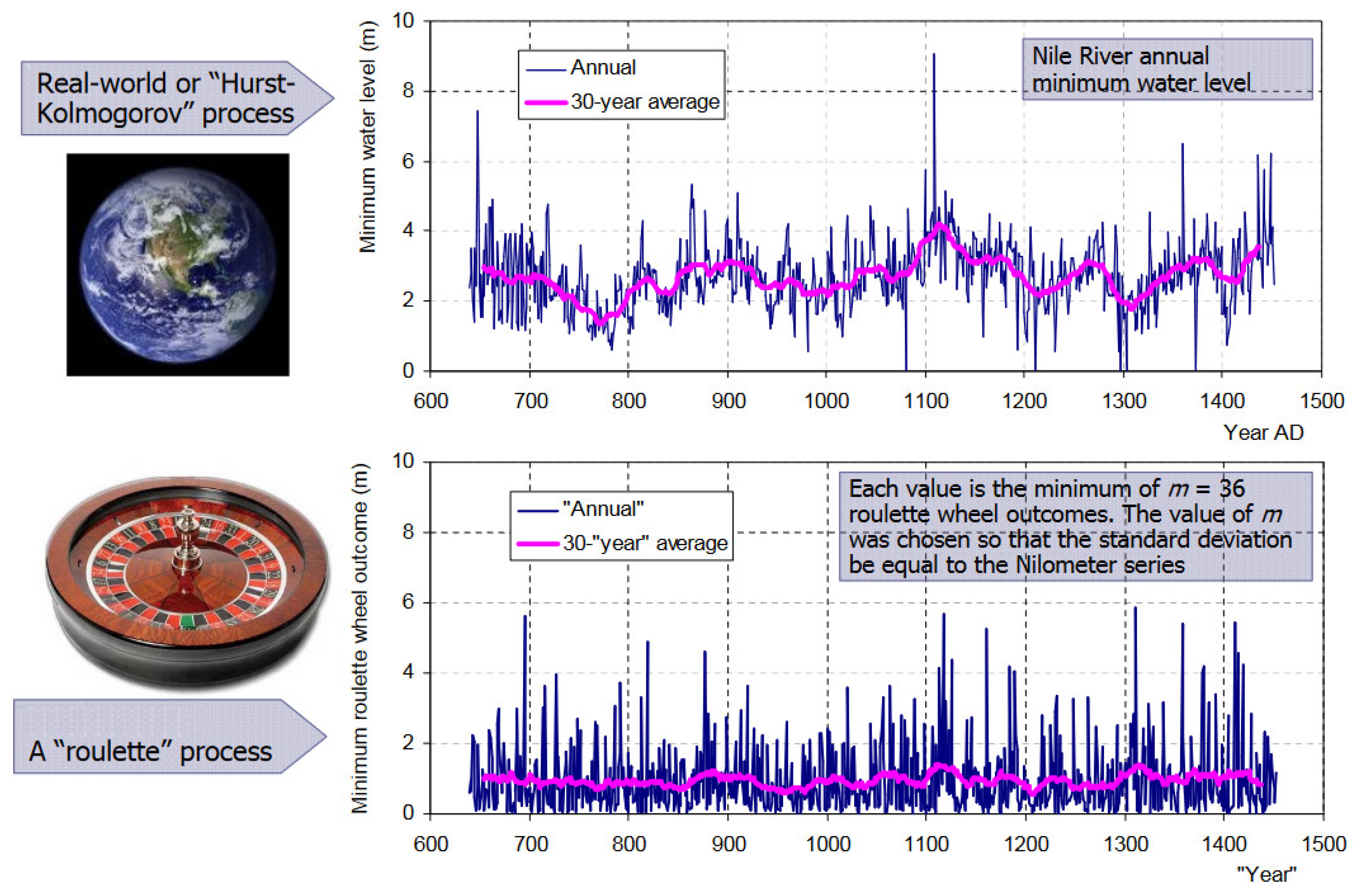
Hurst–Kolmogorov (HK) dynamics present in the annual minimum water level of the Nile River as a result of the perpetual change of Earth’s climate, and as compared to a roulette timeseries resembling a white noise process. Source: [14] (supplementary material).
Figure 2.
Hurst–Kolmogorov (HK) dynamics present in the annual minimum water level of the Nile River as a result of the perpetual change of Earth’s climate, and as compared to a roulette timeseries resembling a white noise process. Source: [14] (supplementary material).

Figure 3.
(a,c) Examples of data series with different statistical characteristics in one dimension. (b,d) Standardized climacograms of the data series shown in (a,c).
Figure 3.
(a,c) Examples of data series with different statistical characteristics in one dimension. (b,d) Standardized climacograms of the data series shown in (a,c).

Figure 4.
Standardized second-order stochastic metrics for the longitudinal velocity of the grid-turbulence dataset: (a) climacogram; (b) autocovariance; (c) variogram; (d) power spectrum. Source: [56].
Figure 4.
Standardized second-order stochastic metrics for the longitudinal velocity of the grid-turbulence dataset: (a) climacogram; (b) autocovariance; (c) variogram; (d) power spectrum. Source: [56].

Figure 5.
Benchmark image analysis; (a) white noise; (b) image with clustering; (c) art painting. Source: [35].
Figure 5.
Benchmark image analysis; (a) white noise; (b) image with clustering; (c) art painting. Source: [35].

Figure 6.
(a) Climacograms of the benchmark images; (b) standardized climacograms (i.e., divided by the variance of the image) of the benchmark images. Source: [35].
Figure 6.
(a) Climacograms of the benchmark images; (b) standardized climacograms (i.e., divided by the variance of the image) of the benchmark images. Source: [35].

Figure 7.
Images of sandstone as seen (a) from the SEM (50 μm); (b) from a polarizing microscope, (3.5 mm); (c) from a hand specimen (with length approximately 5 cm); and (d) from a field outcrop (1 m). For more information on the source, description and processing of the images, see [32].
Figure 7.
Images of sandstone as seen (a) from the SEM (50 μm); (b) from a polarizing microscope, (3.5 mm); (c) from a hand specimen (with length approximately 5 cm); and (d) from a field outcrop (1 m). For more information on the source, description and processing of the images, see [32].

Figure 8.
Standardized climacograms of sandstone images depicted at four different scales and the fitted 2D HK model (source: [32]).
Figure 8.
Standardized climacograms of sandstone images depicted at four different scales and the fitted 2D HK model (source: [32]).

Figure 9.
The image on the left shows Hurricane Sandy from a satellite view (source: www.nhc.noaa.gov/data; accessed on 15 January 2013), on which wind velocity and directions measurements are based. The images on the right represent the wind speed magnitude (in m/s) across a 150 × 150 grid, with 10 km resolution, centralized to the eye of the hurricane observed on (from upper left to lower right) 23, 25, 27 and 29 October 2012 (more details in [40]).

Figure 10.
Climacograms (i.e., aggregated variance of brightness vs. spatial scale in units k × 10 km) for the (a) 23rd, (b) 25th, (c) 27th and (d) 29th day of October 2012. Source: [40].
Figure 10.
Climacograms (i.e., aggregated variance of brightness vs. spatial scale in units k × 10 km) for the (a) 23rd, (b) 25th, (c) 27th and (d) 29th day of October 2012. Source: [40].

Figure 11.
Benchmark of image analysis, the evolution of the universe [68]: (a) 500 million years after Big Bang image with faint clustering, average brightness 0.45; (b) 5000 million years after Big Bang image with clustering, average brightness 0.37; (c) 10,000 million years after Big Bang image with intense clustering, average brightness 0.33. Source: [39].

Figure 12.
Example of the stochastic analysis of a 2D picture, in escalating spatial scales, as shown in red color on the left. The variability of the grouped pixels at different scales are used to construct the climacogram’s images; (a–c) correspond to different time frames as given in Figure 11. Source: [39].

Figure 13.
(a) Climacograms of the benchmark images; (b) standardized climacograms of the benchmark images. A standardized climacogram is not helpful to evaluate the range of the evolution of clustering but is helpful to estimate the curves’ slope for further analysis. Source: [39].
Figure 13.
(a) Climacograms of the benchmark images; (b) standardized climacograms of the benchmark images. A standardized climacogram is not helpful to evaluate the range of the evolution of clustering but is helpful to estimate the curves’ slope for further analysis. Source: [39].

Figure 14.
(a) Cumulative areas underneath each climacogram for each scale; (b) rate of alteration. Source: [39].
Figure 14.
(a) Cumulative areas underneath each climacogram for each scale; (b) rate of alteration. Source: [39].

Figure 15.
Example of image analysis, evolution of the universe (zoomed view): Images of millions of years after the Big Bang (a) 1000; (b) 2000; (c) 3000; (d) 6000. Source: [39].
Figure 15.
Example of image analysis, evolution of the universe (zoomed view): Images of millions of years after the Big Bang (a) 1000; (b) 2000; (c) 3000; (d) 6000. Source: [39].

Figure 16.
(a) Climacograms; (b) rate of alteration of clustering through time. Source: [39].
Figure 16.
(a) Climacograms; (b) rate of alteration of clustering through time. Source: [39].


Table 1.
Climacogram definition and expressions for a 2D continue process, a discretized one, a common estimator for the climacogram and the estimated value, based on this estimator.
Table 1.
Climacogram definition and expressions for a 2D continue process, a discretized one, a common estimator for the climacogram and the estimated value, based on this estimator.
| Type | 2D Climacogram | |
|---|---|---|
| continuous | (T1-1) | |
| discretized | (T1-2) | |
| typical estimator | (T1-3) | |
| expected value of estimator | (T1-4) |
Publisher’s Note: MDPI stays neutral with regard to jurisdictional claims in published maps and institutional affiliations. |
© 2021 by the authors. Licensee MDPI, Basel, Switzerland. This article is an open access article distributed under the terms and conditions of the Creative Commons Attribution (CC BY) license (https://creativecommons.org/licenses/by/4.0/).
Share and Cite
MDPI and ACS Style
Dimitriadis, P.; Iliopoulou, T.; Sargentis, G.-F.; Koutsoyiannis, D. Spatial Hurst–Kolmogorov Clustering. Encyclopedia 2021, 1, 1010-1025. https://0-doi-org.brum.beds.ac.uk/10.3390/encyclopedia1040077
AMA Style
Dimitriadis P, Iliopoulou T, Sargentis G-F, Koutsoyiannis D. Spatial Hurst–Kolmogorov Clustering. Encyclopedia. 2021; 1(4):1010-1025. https://0-doi-org.brum.beds.ac.uk/10.3390/encyclopedia1040077
Chicago/Turabian StyleDimitriadis, Panayiotis, Theano Iliopoulou, G.-Fivos Sargentis, and Demetris Koutsoyiannis. 2021. "Spatial Hurst–Kolmogorov Clustering" Encyclopedia 1, no. 4: 1010-1025. https://0-doi-org.brum.beds.ac.uk/10.3390/encyclopedia1040077