Noise Events Monitoring for Urban and Mobility Planning in Andorra la Vella and Escaldes-Engordany

Abstract

Noise pollution is a critical factor and it has an important impact on public health, with the relationship between road traffic noise (RTN) and several illnesses in urban areas of particular concern. Andorra is currently developing a national strategy regarding noise pollution in their urban environments. The Ministry of Environment, Agriculture and Sustainability is trying to to identify, monitor, map and model the effects of noise pollution and design mitigation policies to reduce the impact in certain priority areas. This analysis should take into account the existence of different types of anomalous noise events (ANEs) present in the street, e.g., horns, people talking, music, and other events that coexist with RTN, to characterize the soundscape of each of the locations. This paper presents a preliminary analysis considering both the Signal-to-Noise Ratio (SNR) and the duration of the ANEs to evaluate their presence in urban areas in the three different locations in Andorra la Vella and Escaldes-Engordany. The experiments conducted required a 10-h recording campaign distributed in the three locations under study, which was evaluated on two different days, one during the week and the other on the weekend. Afterwards, the data were carefully labeled and the SNR of each event was evaluated to determine the potential impact of the four categories under study: vehicles, works, city life and people.

1. Introduction

Noise is one of the major issues in big cities, especially noise coming from traffic, which is one of the main pollutants in urban and suburban areas that affect the quality of life of citizens [1]. However, even more important is the fact that it also has an impact on their health, and can cause health issues such as lack of concentration, sleep disturbance and stress [2]. The problem is increasing as cities grow both territorially and in population, making it a more pressing issue for city councils. Several studies have been conducted in order to prevent and cut down the negative effects of this traffic noise exposure on the population [3].

Several European countries have reacted to this alarming increase of environmental noise pollution by approving the directives issued by the European Noise Directive (END) [4], which advocate the creation of maps to inform citizens of their exposure to noise and preparing action plans to reduce the impact of noise pollution [5]. These maps are represented using the equivalent noise level ($L_{DEN}$) and require an expensive and time consuming process carried out by local governments, and the resulting actions can only be implemented and evaluated every five years. Historically, these maps have been created using certified devices, based on short periods of time and have been designed to be as representative as possible.

Nevertheless, this classic method is becoming obsolete given the new paradigm created by the Wireless Acoustic Sensor Networks (WASNs) [6]. WASNs have been developed under the paradigms of smart cities and the Internet-of-Things (IoT). Furthermore, WASNs are being used to manage city noise, which include noise mapping, developing action plans or increasing population awareness among others [7]. For instance, the project SENSEable [8] proposed a WASN to collect acoustic information in Pisa (Italy) using low cost acoustic sensors to study the relationships among public health, mobility and pollution caused by citizens’ behavior. Some of the projects that have adapted a similar position are the IDEA Project in Belgium [9], the RUMEUR network in France [10] with a special emphasis on aircraft noise, the “Barcelona noise monitoring network”, which is integrated in Sentilo in the management platform of the city [11], or the DYNAMAP project, which has the objective of developing a dynamic noise map, capable of detecting and representing the acoustic impact of road traffic noise (RTN) in real time in the cities of Rome and Milan (Italy) [12].

Nowadays, the combined population of Andorra and Escaldes-Engordany is roughly 40,000 inhabitants, but this number increases during August and the winter season, when people visit its ski resorts and consequently there is a significant increase in traffic. This project aimed to be an initiation to noise monitoring in Andorra to provide an idea of the problem and determine whether its impact is relevant enough to be controlled and monitored. The Government of Andorra started monitoring acoustic pollution levels across the country in 2009, using a quality indicator with a similar scale as defined in [13,14], as well as the soundscape ISO technical specifications [15]. The information published in the report only states that these indicators are based on the measured values and a zoning of different levels of sensitivity based on the potential activities to be affected (residential, leisure, etc.).

Andorra, as a non-EU country, is not required to apply and implement the END or any other European Directives. However, the government tends to deploy regulations and frameworks following most of these European regulations usually with slight changes to take into account the particularities of the country. Thus far, for this specific case, the Government of Andorra implemented the regulation for the control of the acoustic pollution in 1996 [16]. The regulation states that maximum levels allowed from emitting sources are 65 dBA during the day and 55 dBA at night. In non-industrial areas (e.g., residential, commercial, etc.), the maximum allowed levels are 55 dBA during the day and 55 dBA at night. Maximum reception levels allowed inside residential buildings cannot be higher than 35 dBA during the day and 28 dBA at night; nevertheless, in common areas, higher values are allowed. In dorm rooms, these values have to be at maximum 30 dBA during the day and 27 dBA during the night. In 2017, the statistics were of very good quality with 52% of the records measuring excellent conditions, 37% good conditions and only 11% moderate and bad conditions (The criteria used to determine the excellent, good, moderate and bad conditions is contained in a private document owned by the Government of Andorra.) The average values of Andorra la Vella stated that 8% of days had bad conditions and around 30% of days had moderate conditions [17]. These spots correspond to the most touristic and crowded areas in the country, combined with the roads with the highest traffic density.

On the other hand, the National Strategic Plan of Tourism and Commerce 2015–2019 [18] fixed the goal of developing a sustainability label and improving most of the sustainability indicators related to the impact and experience of tourism together with the Ministry of Environment. In this context, the improvement of the quality of the acoustic environment and a reduction in the exposure of both locals and tourists in order to improve their quality of life and tourism experience have been fixed as a short-term objective. Andorra is currently developing a national strategy regarding noise pollution. In this line, the Ministry of Environment, Agriculture and Sustainability is aiming to identify, monitor, map and model the effects of noise pollution and design mitigation policies to reduce the impact in the determined priority areas.

The present study aimed to be the first step to better understanding the acoustic pollution dynamics in some of the spots with the poorest acoustic quality according to the reports of the official monitoring statistics. Thus far, the official measures have only considered levels of noise pollution [17], and no noise typology has been considered leisure, traffic, etc. However, even though traffic is one of the most important sources of noise in the area, other sources make an important contribution. In this study, besides the measurements of level of noise $L_{Aeq}$ in the points of study, the identification and measurements of the contributing sources were obtained. This study added a new dimension in the analysis and created a better understanding of the dynamics in the area, where the contributing sources can change over time. Its results set the basis for a deeper analysis of the three key locations, and paves the way for future effective interventions and mitigation actions in accordance with the results in order to improve the quality of life in these areas.

This paper is structured as follows: in Section 2, a brief state of the art of noise monitoring is described. In Section 3, a description of the pilot areas and the on-site recording campaign is provided. In Section 4, an analysis of the events present in the recording campaign is detailed. In Section 5, the future lines to be developed in Andorra and Escaldes-Engordany are discussed.

2. State of the Art of Noise Monitoring

In response to the requirement for automatic noise measurements in urban areas, WASN-based projects are being carried out in several countries. Furthermore, some of these projects also include other environmental measurements. In this section, we describe several approaches deployed to automatically conduct the noise measurements in cities in order to obtain noise maps [19].

One of the very first reports in the literature about the wireless acoustic sensor networks (WASNs) was by Telos [20]. An ultra-low power wireless sensor module is introduced, designed for research and experimentation in the Wireless Sensor Networks (WSNs) area and developed by the University of California, Berkeley, which became the leading reference in the investigation in automatic environmental monitoring. In [21], Santini et al. also proved the possibility of using a WASN in a vast number of environmental monitoring applications, in order to monitor the environmental noise pollution in cities [22]. In [23], the authors described the deployment of a WASN with the objective of measuring acoustic noise in residential and industrial surroundings in Ostrobothnia (Western Finland). All of the sensor nodes evaluate the $L_{Aeq}$ noise level at its current location, and the information is processed into a web-based database.

In the SENSEable project [8], a WASN was used to gather information about the acoustic environment of the city by means of low-cost acoustic sensors with the final goal of studying the relationship between public health, mobility and pollution by observing the citizens’ behavior, obtaining promising results about the anthropogenic component not revealed by public strategic maps. Bartalucci et al. explained [24] how Monza project expects to carry out noise measurement activities in a pilot area using sound level meters of Class I precision through the development of a low-cost system. There are also several networks based on commercial sound level meters, such as the one used in Xiamen City (China) to monitor traffic noise [25]. The designed WASN also considers ZigBee technology and GPRS communication, and all the nodes of the network use the same type of device.

The Fi-Sonic project is based on the emerging IoT applied to the smart city concept, building low-cost acoustic sensors to deliver real time specific sound features capable of determining the location of sound sources for security and surveillance purposes [26]. The CENSE project [27] aims at proposing a new methodology for the production of more realistic noise maps due to the questionable relevance of the maps set out by the European Directive 2002/49/EC, based on an assimilation of simulated and measured data, collected through a dense network of low-cost sensors.

The RUMEUR platform developed by BruitParif (Urban Network of Measurement of the sound Environment of Regional Use) has three objectives: understanding phenomena, assessing actions against noise and openly and directly communicating information on the sound environment in Ile-de-France, especially focused on aircraft noise. One of the goals of the DYNAMAP network was to achieve a good trade-off between cost and accuracy in the WASN design [12,28]. This project has already deployed two pilots in Rome [29] and Milan [30], to evaluate the noise coming from road infrastructures in suburban and urban areas, respectively.

In Barcelona, Spain, an environmental noise monitoring network was set up for the purpose of managing resources efficiently in order to reduce the impact of urban infrastructures on the environment [11]. Once the deployment of the network was successful and had been working for some time, the Barcelona Noise Monitoring Network (NMN) performance was newly reviewed to establish its weak points, strong points and to define future open challenges [31]. In [32], the UrbanSense project attempts to monitor real-time urban noise together with other air pollutants in Canada. The infrastructure was designed in a scalable way, including a wide range of outdoor sensors combined with a data aggregation system and a web-based data management and visualization application with the goal of showing real-time event-based information integrated in a single platform.

The IDEA (Intelligent Distributed Environmental Assessment) project [9] in Belgium uses new capabilities offered by consumer hardware to deploy sound monitoring methodologies that imitate human environmental sound perception as closely as possible. The MESSAGE (Mobile Environmental Sensing System Across Grid Environments) project [33] monitors noise, pollution and air quality in addition to traffic flow, supplying real-time data in the United Kingdom. They are both focused on the use of a single-board computer with low computational capacity and even using low-cost sound acquisition cards. This idea allows the deployment of a large number of nodes network, increasing the number of sensed locations in the city.

Other issues have to be taken into account for a proper design of a WASN and the evaluation of its measurements. Following the idea of the real-time monitoring of city environments, several works have focused on the assessment of the impact of human activity on environment and human health [34]. In the field of information processing and evaluation, spatial integration of measurements is also a big issue [35], as is the influence of contextual factors [36]. Furthermore, this last work considers the possibility of participative monitoring by the citizen, which is also considered and evaluated in [37,38], but the accuracy of the results depends on the devices and the number of measurements. The approximation of noise mapping to the real perception of the people is also an issue to study deeply once one a good measurements system has been deployed [39,40].

3. Pilot Areas On-Site Recording Campaign

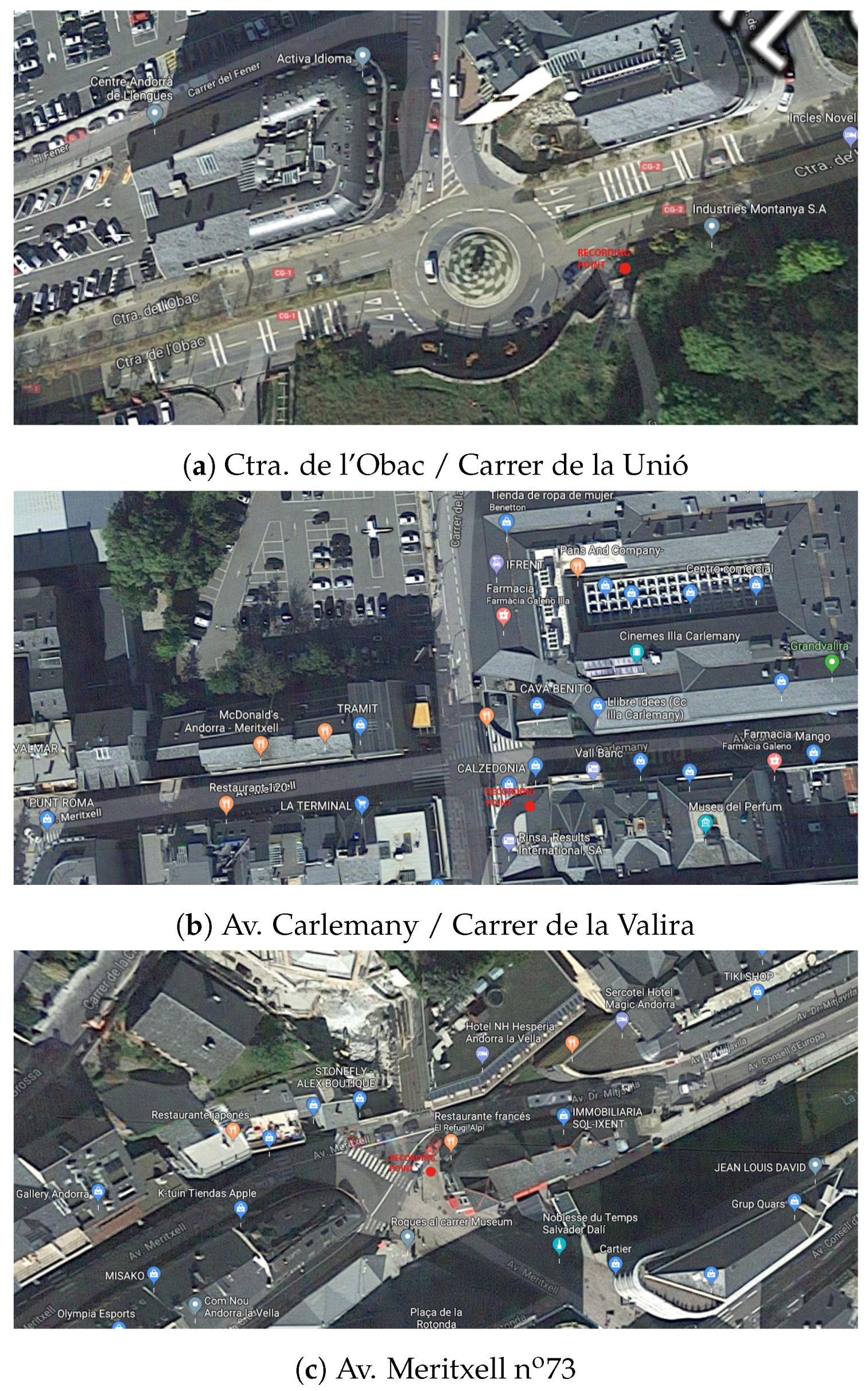
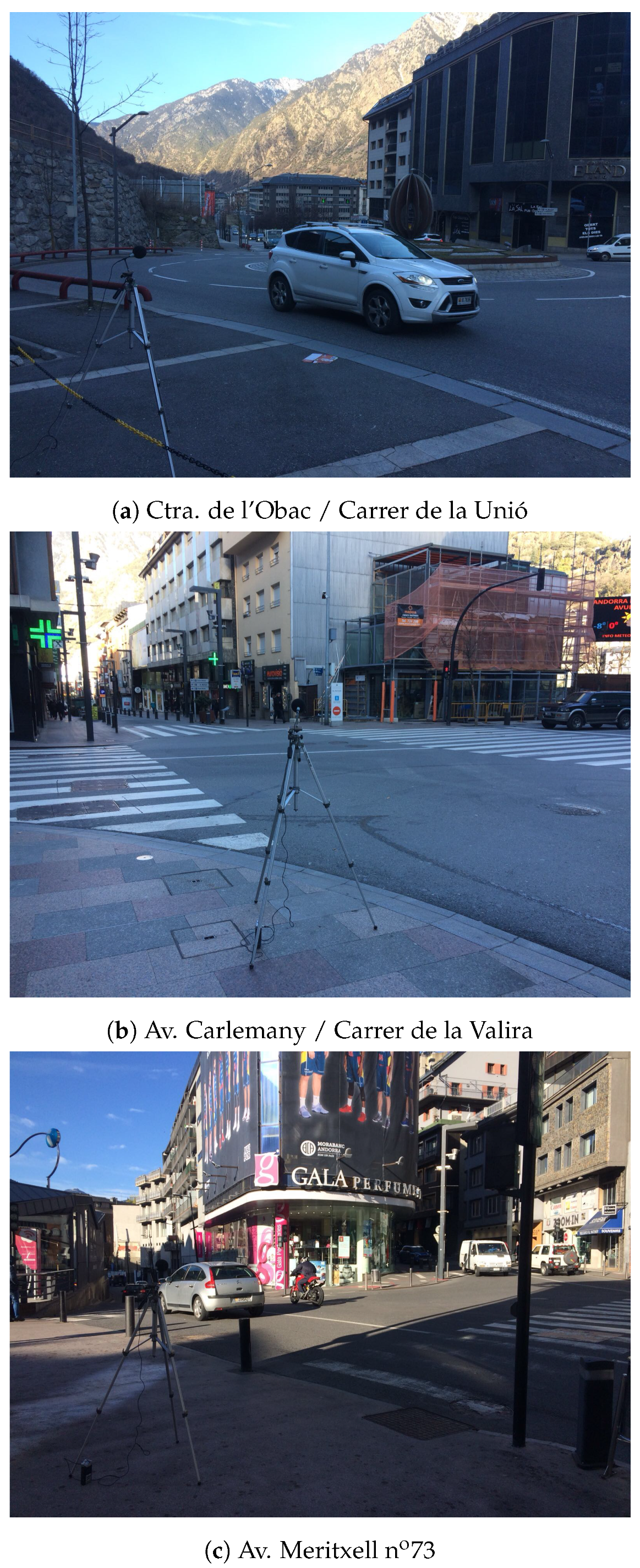
In this section the areas of the three measuring locations are described in Andorra la Vella and Escaldes-Engordany, together with the reasons that guided the choices, mainly related to the results of preliminary analysis with automatic level meters deployed in several critical locations in the country. The first one corresponds to a residential area near a speed-road, the second one to a mostly pedestrian and commercial area, and finally the third one is a touristic area close to dense traffic. Details about the instruments used to carry out the recording campaign and the sampling design schedule used are provided.

3.1. Locations

The selected measuring locations correspond to three important nodes in terms of volume, both for pedestrians or for vehicles. Location (a) (see Figure 1a) is the connection between the country’s three main roads in the capital [16,41], with the highest traffic congestion experienced during rush hours. In this area, the main sources of noise are expected to be cars. This is expected to have constantly high levels of noise and a lower variability in terms of contributing sources compared to other areas. Location (b) (see Figure 1b) is the intersection between CG-3, the road leading traffic from the capital to the north valley, with the main pedestrian and commercial axis, one of the most frequented points by tourists. In this area, the mix of potential sources of noise should be higher, as should the variability of contributing sources of noise in different days or during the day. This location is of additional interest due to its recent transformation into the biggest pedestrian zone in the country. Location (c) (see Figure 1c) is also the intersection of an important road and the pedestrian axis, sharing the same interest for the study as Location (b). Compared to Location (b), in this case, the axis is not fully pedestrianized but with an intervention of reducing and slowing the traffic. In this case, the variability of the sources should also be higher during the day. In this case, the impact of two different types of urban intervention is expected to produce different noise dynamics in the area. Thus, these three locations were chosen to analyzse noise source identification. Furthermore, these are the most likely places to prioritize future interventions and mitigation measures.

The recordings took place on 2 March and 15 April of 2018. The reason for recording on these two specific days was to collect a database of audio recordings during a weekday as well as a database recorded during the weekend. With these results, we attempted to see a difference in the results and detect which are the noisiest areas, when and why, of the universe of two entire days of data recording. Day 1 was cloudy and windy with an average temperature of 0 ${}^{\circ }$C, while Day 2 was sunny with an average temperature of 13 ${}^{\circ }$C. As previously mentioned, the three places were carefully selected to cover crowded areas in terms of traffic (see Figure 2a,c) and for people (Figure 2b). While Figure 2c is inside the city and has traffic lights, Figure 2a is a road where cars reach higher speeds and there is only one roundabout to slow vehicles, creating higher impact. On the other hand, Figure 2b is characterized by human noises for it is in the middle of the city and has less traffic since it is partially pedestrianized. As evidence that these are crowded areas in terms of traffic, it should be noted that during Day 1, 45.39% of labels used belong to Vehicles, and during Day 2, 43.42% were used for Vehicles. The labeling system is detailed in Section 4.

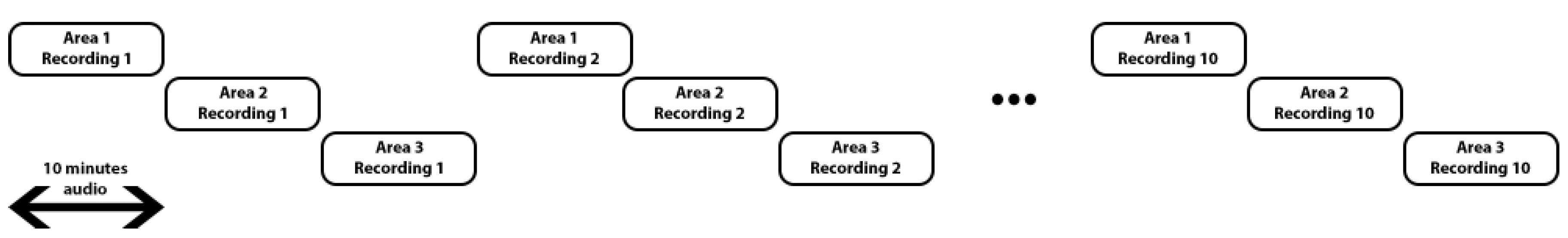
3.2. Material and Methodology

To conduct the recordings, a ZOOM H4n digital recorder [42] was used. The sensor was placed on a tripod at a height of 1.5 m and with an inclination of 45${}^{\circ }$, and the tripod was placed 5 m from the targeted area to be recorded and 2 m from any wall behind the device, as can be observed in Figure 2. This methodology was applied for the three recording locations taking into account particularities from each location, but maintaining the criteria for all recordings during the two days.

A 94 dBSPL, 1 KHz calibration tone was used at the beginning and at the end of every recording to verify its sensitivity and ensure the correct performance of the sensor. Each recording lasted between 11 and 12 min to guarantee at least 10 min of usable audio, assuming that this value could give us the $L_{Aeq}$ for 10 min and also a diversity of events to detect in each location. With only one set of equipment available, the three areas could not be recorded simultaneously, hence we started at 08:00 in the first location. When the first recording was conducted, we headed to the second area, and then to the third. This was repeated up to 10 times, thus, for each day, 30 audio recordings at 48 KHz were collected. Each round took almost 1 h, which was the second reason to choose 10-min recording. Figure 3 shows a visual description of this iterative process of recording. To stick close to the original goal of recording simultaneously the three areas, and to be as rigorous as possible, this sequential method was chosen to emulate the initial idea, taking into account that there is a slight delay between the end of one recording and the next start as all the equipment had to be moved. It is important to mention that all the recordings were supervised by a technician, and notes were taken by hand to have a reliable sample set of any noise event that could be misleading during the post-processing, and also to make it more consistent and easier to leave out overlapping sounds.

4. Analysis of the Acoustic Events Present in the Recording Campaign

After the recording campaign, the noises of each area were analyzed to evaluate common events and noise dynamics. To classify them, four categories were decided by the Observatori de Sostenibilitat d’Andorra (OBSA) and Actua. Traffic played an important part in all three recording areas, so a category for all kind of Vehicles was required and it was the one with most labels. Besides Vehicles, already expected to be one of the main sources of noise in all three pilot areas, three other classes were considered in the analysis. People was classified as any noise made by persons, because two of the three pilot areas are highly frequented places for tourists, with crossing points for pedestrians (Location (b)) or half-pedestrian (Location (c)) areas. In this line, City Life class, as any noise taking place in an urban area but omitting traffic noise, was also used due to expected noises coming from urban elements such as traffic light emitters or street music. Finally, some construction works were carried out in places near the measuring pilot areas, thus the Works category was also considered. Moreover, once the dynamics of these four categories had been identified in the pilot locations, the information could be focused on the design of specific measures to mitigate the impacts on the quality of the environment.

• Vehicles: All noises coming from any mean of transport, not necessarily having an engine.
• Works: All noises related to construction jobs.
• City Life: Any noise taking place in an urban area excluding vehicles.
• People: Any noise made by a person.

Brief descriptions of labels used in this study are presented below.

• alrm: noise of car alarms.
• bark: dog barking.
• beep: noise of a crane or a truck going backwards.
• bell: noise of a bell.
• bike: noise of bikes.
• bird: birdsong.
• bldz: noise of a bulldozer.
• brak: noise of vehicles brakes.
• cano: noise of a can being opened.
• clap: noise of hands clapping.
• coug: person coughing.
• cptr: noise of a compactor.
• door: opening or closing noise of a vehicle door.
• drll: noise of drilling.
• dryb: noise of a dry blow.
• heli: noise made by helicopters propellers and engine.
• horn: horn vehicles noise.
• lves: noise of dry leaves on the floor.
• mbke: noise of motorbikes.
• mblw: noise of a metal blow.
• meca: noise of a metal can falling on the floor.
• musi: music coming from the street or a vehicle.
• pbag: noise of a plastic bag being moved by wind on the floor.
• peop: people talking.
• phmr: noise of a pneumatic hammer.
• quad: noise of a quad.
• radi: noise of a radial cutting.
• rtn: road traffic noise, used as background label during this project.
• scar: noise of sports car speeding up.
• sctr: noise of scooter wheels.
• shvl: noise of a shovel.
• shout person shouting.
• sire: noise made by an ambulance or police car siren.
• skte: noise of skate wheels.
• snze: person sneezing.
• stfs: strong falling noise.
• strt: engine noise while starting a car.
• swrl: noise of a vehicle passing over a sewer lid.
• tlbp: traffic light beep (adapted for blind people).
• trck: noise of trucks.
• trll: noise of a wheeled suitcase.
• walk: people walking without talking.
• wata: people talking on a walkie-talkie.
• whst: person whistling.

The final classification for all labels divided into the four categories explained in Section 4 is detailed in

Table 1. All labels used at least once during the post-processing stage.

Noise Events Category List
Vehicles	Works	City Life	People
alrm	beep	bell	cano
bike	bldz	bird	clap
brak	cptr	bark	coug
door	drll	bkmu	keys
heli	dryb	lves	peop
horn	mblw	meca	shout
mbke	mtlf	musi	snze
quad	phmr	pbag	walk
rtn	radi	swrl	wata
scar	shvl	tlbp	whst
sctr	stfs	trll
sire
skte
strt
trck

.

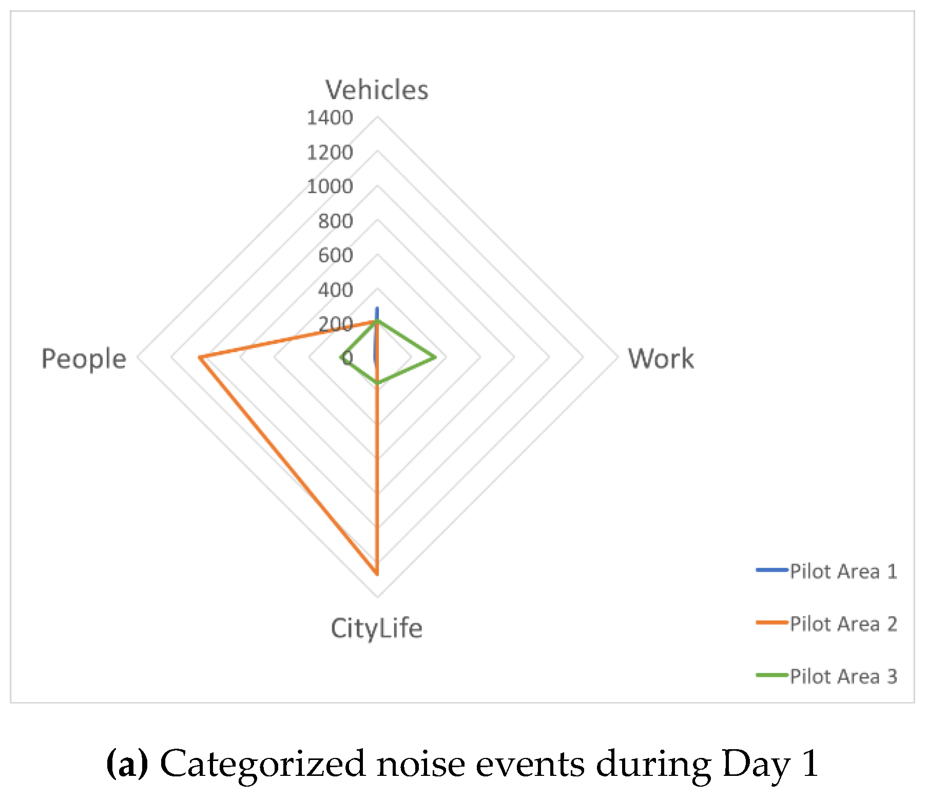
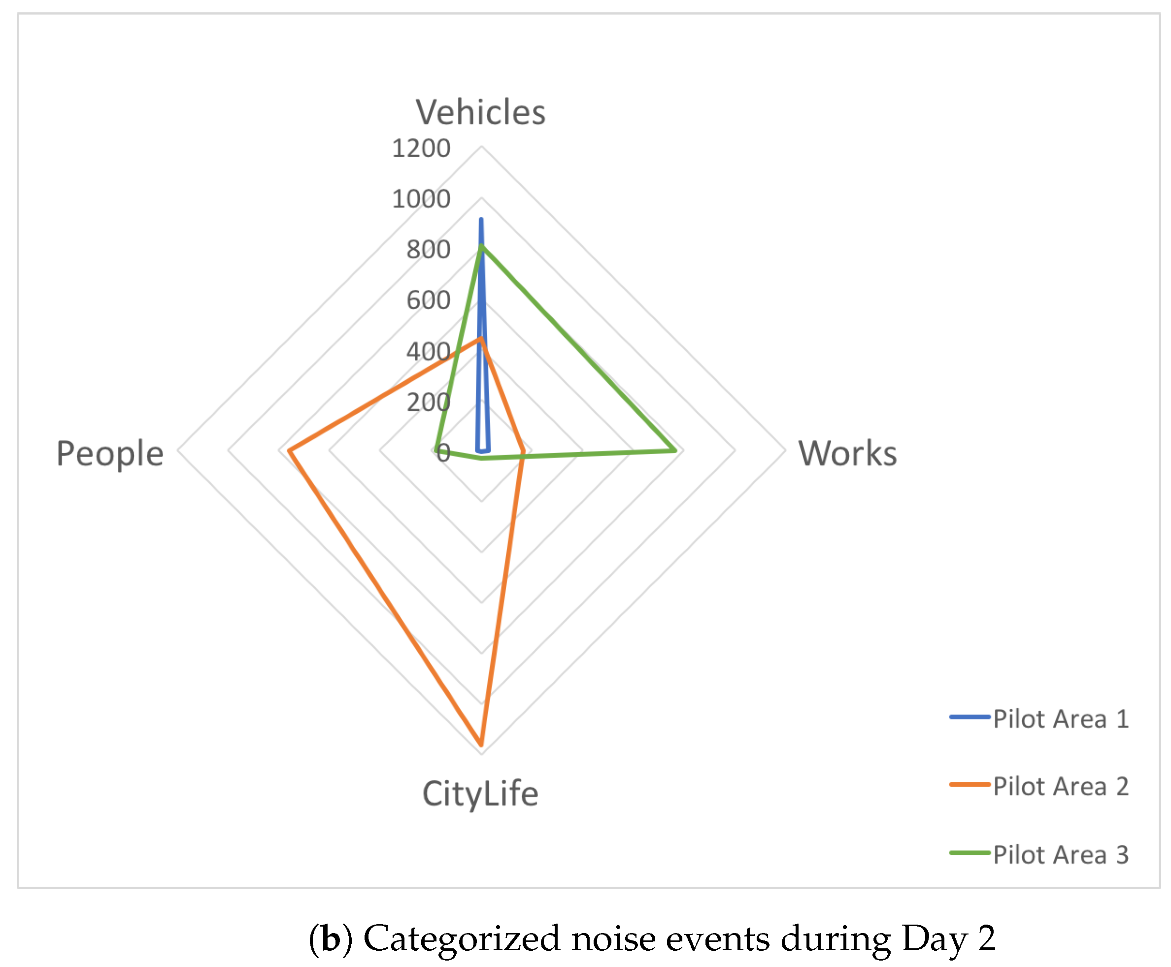
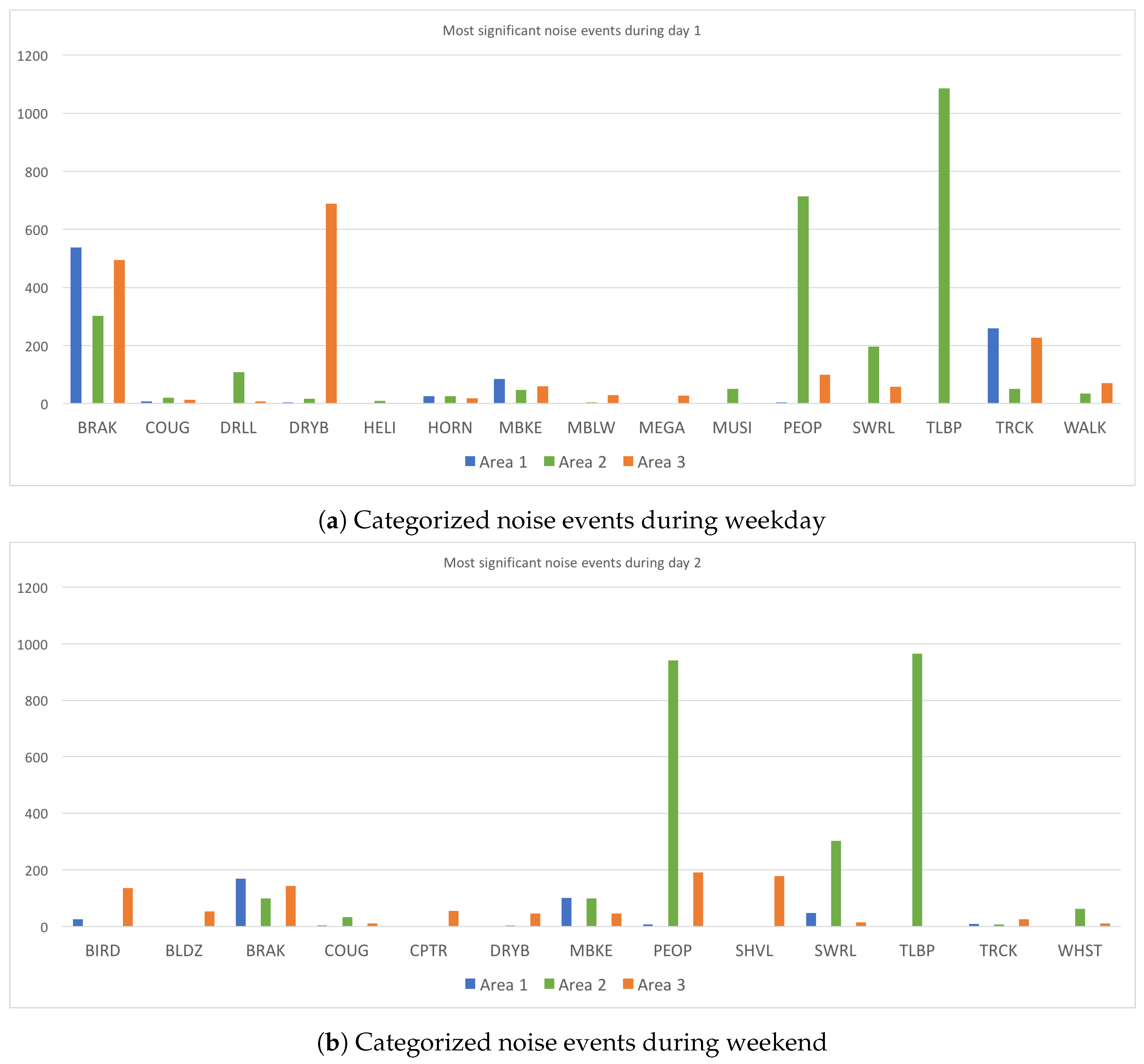
4.1. Event Occurrences

We analyzed the presence of different types of noise at each of the locations. The four categories are displayed in a radar plot. In Figure 4, the aggregated time recorded for all events in the three locations is shown for both days. Basically, Pilot Area 1 always contains noise from vehicles, and some works, but no more sounds associated to city life or people, neither during the week nor on the weekend. Pilot Area 2 corresponds to the semi-pedestrian zone, and contains mainly city life and people, followed by works due to a water leakage and some vehicles. Finally, Pilot Area 3 registers mainly works, some people and vehicles, corresponding to the description of the location.

Figure 5 shows the detail of the occurrences aggregated in Figure 4 by type of sound, location and day of the week.

As stated in Figure 5, Pilot Area 2 is the only one with adapted traffic lights for blind people, hence this event only exists at this point. Comparing Figure 5a,b, it is clear that during the weekend there is barely any traffic in any of the pilot areas and the total number of cars dramatically decreases with the reduction in brake and horn labels a good indicator of this fact. On the second day (Figure 5), in Pilot Area 3, a water pipeline broke leading to sudden Works that lasted for over half of the recording time, which also affected regular traffic as the road was blocked. Events such as shvl, cptr or bldz appear exclusively there due to this rare event but would not normally take place. We can also state that, in Figure 5, Pilot Area 1 is a purely traffic area since there was a very narrow sidewalk on which practically nobody walked. The amount of People recorded on both days is similar, but the difference lies in the times when they were recorded. On Day 1, the vast majority of them took place when kids finished school or adults left work while during the weekend it was more balanced throughout the whole day.

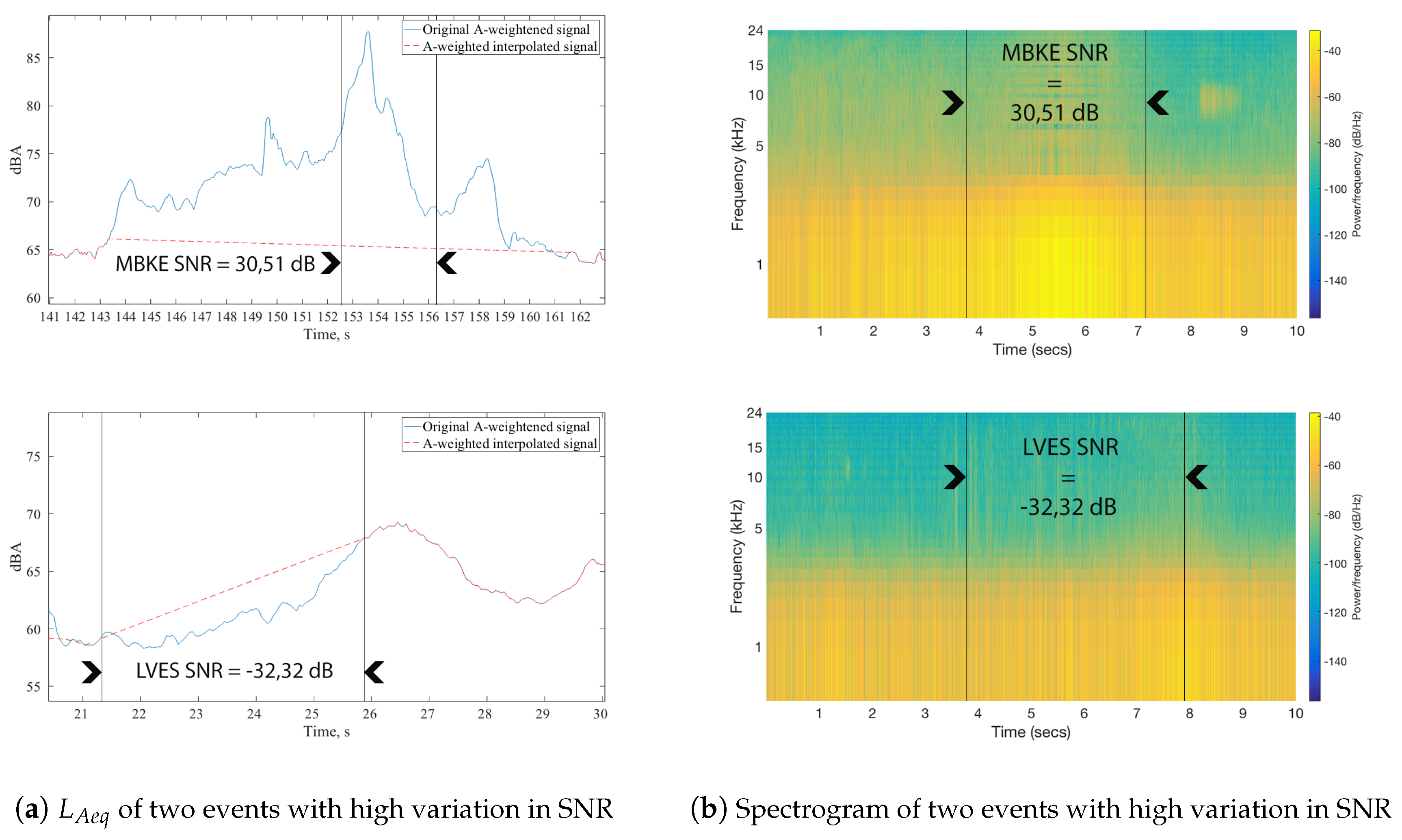
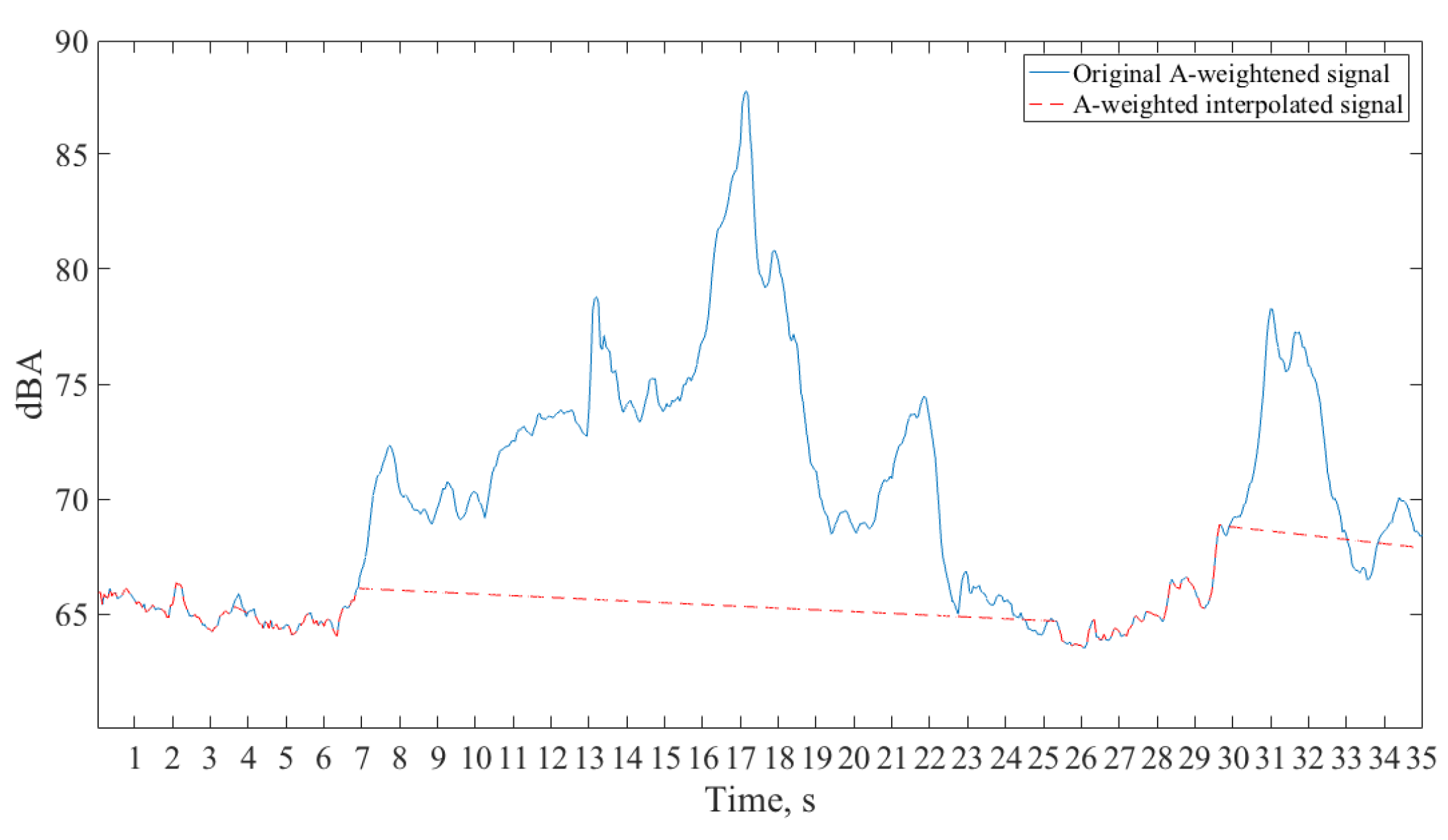
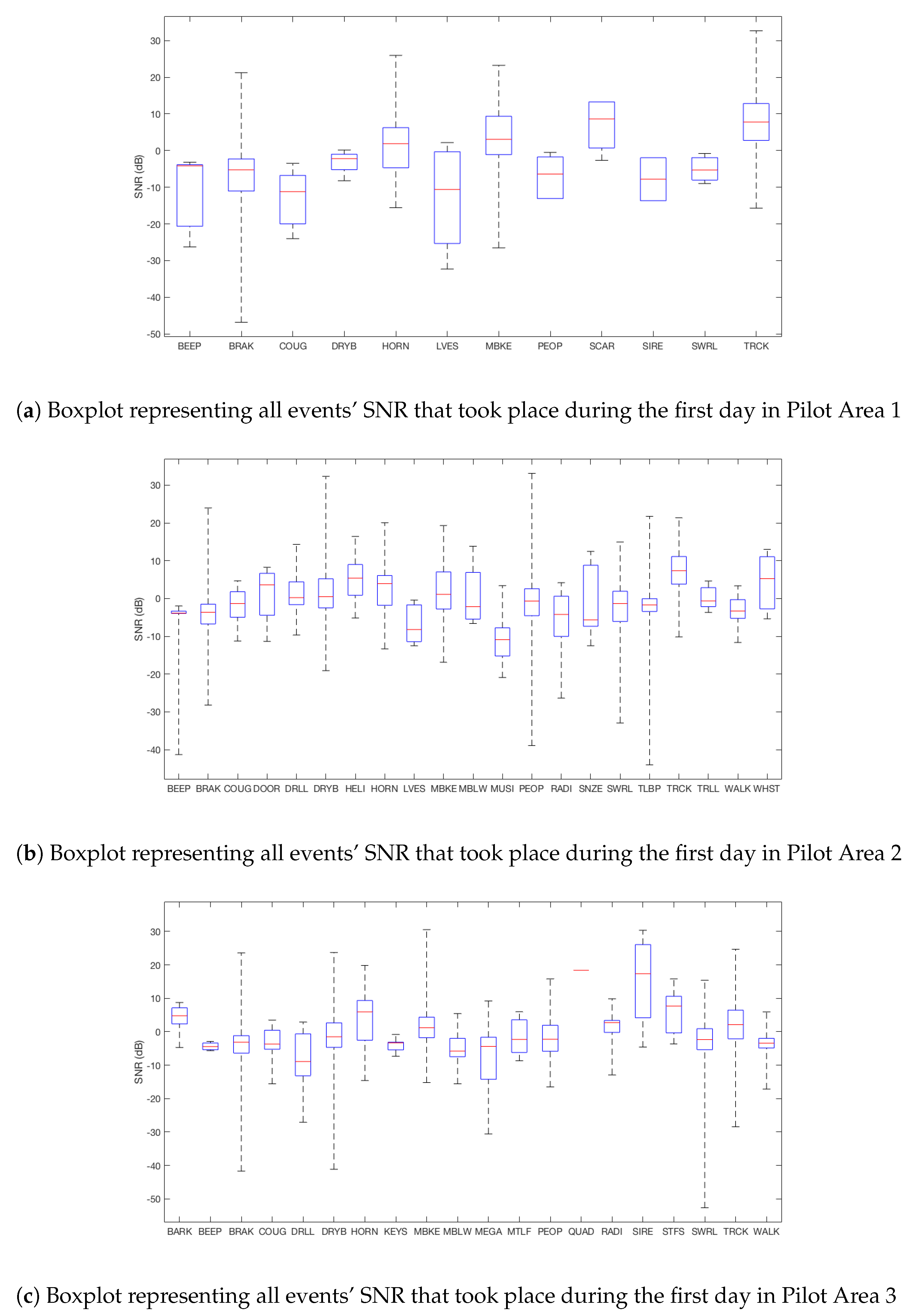
4.2. Events Signal to Noise Ratio Evaluation

In this section, an exhaustive analysis of the noise events shown in Section 4 is described. Together with SNR, we provide a wide view on what are each region’s most significant problems in terms of acoustic pollution.

• SNR: It is defined as the relation between the power of the noise event being evaluated and the previous and posterior RTN power of that given event. The following equation explains how it is calculated [43].

$$P_x=\sum _{t=1}^N\left(\frac{x{\left(t\right)}^2}{N}\right),$$

(1)

where N is the number of samples and $x\left(t\right)$ is the event we want to calculate its power. Once this is done, SNR is computed as stated in its definition.

$$SNR=10lo{g}_{10}\left(\frac{P_{NE}}{P_{RTN}}\right),$$

(2)

where $P_{NE}$ matches the noise event power and $P_{RTN}$ stands for the previous and posterior RTN to that event. It is worth noting that, when calculating both powers, it is not strictly necessary for N to be the same size, since it is a summation that will be divided by N in the end. Furthermore, it can be observed that some events will have a negative SNR. This can happen due to high traffic noise that makes an event irrelevant despite being clearly audible.

There is a large amount of events with a negative SNR value mwhich can either mean that the surrounding vehicle noise was louder than the labeled noise or that the event itself was very weak. Whatever the reason, these events are not relevant in the specific moment they took place as they do not represent an impact on humans even though they can be heard.

Figure 6a shows two events that took place at different locations during the same day and have similar duration, but have a dramatic contrast in terms of SNR. The first noise belongs to a motorbike that lasts for 3650 ms and has a 30.51 dB SNR and the second one to dry leaves on the ground moved by wind gusts of for 4250 ms with a −32.32 dB SNR. Figure 6b presents the same events as spectrograms. Both events can be extrapolated to most of the labels and do not follow a certain pattern since a brake can have a minimum SNR when its surrounded by other vehicles or a medium or even high SNR in a calm environment.

The spectrograms can be seen as a more visual way of detecting a high SNR through an event’s spectral power density when represented in colors. The spectrogram also offers the possibility of seeing at a glance to which frequency band the event belongs through the sharpness of the colors. In the mbke event, even though there is a stronger presence between 5 KHz and 24 KHz, it is not relevant but the low frequency part where we can detect a condensation without any effort showing that this is the margin where the event is taking place. Moreover, in the first area, if leaves had not been labeled, it would have been impossible for anyone to detect any kind of event between the marked boundaries.

As detailed in Equation (2), SNR is the relation between the noise event and two RTNs which are always intended to be as nearby as possible from the event. It can be appreciated in Figure 7 that the RTN after the noise event happens with no other event in between. On the other hand, there are other frames that have to be avoided when calculating the SNR between $RT{N}_1$ and the motorbike event. For this process to be meaningful, a careful labeling process was imperative r to guarantee that the SNR was a reliable measurement.

In Figure 8 the average SNR for most of the labels used in the three pilot areas are presented during the first day. Through these boxplots, the SNR limits of all events can be appreciated. Readers may notice how patent it is that Pilot Area 1 barely has any human activity and most of the labels belong to Vehicles category. Out of the twelve labels used in Pilot Area 1 post-processing, 50% of them corresponded to Vehicles. It is also worth mentioning that, despite having a clear average, all events have both positive and negative peaks, and those above average due to their impact on humans are more important for this study. These peaks occur due to environmental quietness, especially visible in the brake label in the three pilot areas, whereas tlbp, only present in Pilot Area 2 is also a clear example. In addition, the proximity of the event to the sensor makes a noticeable difference in any noise, but especially in those which would normally still have a high SNR regardless of the distance, such as horn. As a conclusion, Pilot Area 2 depicts quite different values from the other two areas, and this is probably because it is the most commercial and pedestrian zone measured, i.e., the one where the traffic noise had less impact on the measurements.

5. Discussion

The government is currently working on national strategies to identify, monitor, map and model the effects of noise pollution and design mitigation policies to reduce the impact in priority areas. These first monitoring campaigns permitted us to explore the potential of measuring noise pollution in different areas of the city to better understand urban dynamics during a given day, in order to plan deeper studies considering also the meteorological conditions throughout the year. The recording campaign should be expanded throughout the year to obtain data from different meteorological conditions. One of the goals of the Andorran Government and the municipality of Escaldes-Engordany is to create a system of real-time monitoring and data integration of different sources of information to inform about the urban dynamics such as traffic and pedestrian patterns, energy consumption, environmental pollution among others. The preliminary recording campaign and analysis presented in this study permitted us to explore the potential to integrate and cross noise information of different locations of the city in order to better understand what are the different sources that are impacting the most the citizens and tourists, and what are their spatial and temporal dynamics. First, the inclusion of this kind of information in the integral “single-view” system of the city can help us to better understand the most important drivers and their dynamics that lead to an increase in noise pollution. Second, these data analyzed together with different sources of information can provide relevant results to design more suitable policies, measures and urban interventions to reduce noise pollution in the areas where a higher number of citizens and tourists are exposed to, and can help in the objective from both the government and the municipality, to increase the environmental quality and the welfare of these groups.

Further work will be devoted to developing a longer measuring campaign that deploys in parallel with other devices such as cameras to apply computer vision to continuously record metrics about the events that occurred during the measurements periods and spanning a greater period to capture other dynamics such as day-night and inter-daily variability. Finally, a further process to identify other measurement points that can reproduce other events and dynamics that were not represented in the current points should be carried out to finally design efficiently a potential network of permanent measurement points, and the parallel data required to gather in order to visualize in the City data Platform the relevant information. It is relevant, therefore, for a future intelligent type of noise monitoring system in Andorra, to bear in mind that there will be a wide variability of samples of noise registered in the different locations, and, therefore, each class will also have a different impact on the population. Thus, the automatic detection [44] of the four types of noise defined in this work could be crucial for a suitable design of the noise map, for further epidemiological studies over population [43]. The final goal is to model the noise pollution and achieve a layer of information relevant to better inform about the impact analysis of particular events and periods and improve the decision-making processes of the city.

6. Environmental Policies Involved

The only law regarding noise management in Andorra is the one about environmental and acoustic pollution [41] and the regulation of control of acoustic pollution [16]. This regulation defines the maximum permitted thresholds for the municipalities to control and take measures when achieved. Moreover, the Andorran Government and the different municipalities are working to create the national acoustic register. Nowadays, this cadaster is based only on acoustic levels. Thus, this work can contribute to starting to explore the impact of the diversity of noises in the different areas of study and the potential interest to include these kinds of measures in the acoustic cadaster.

References

1. World Health Organization (WHO). Environmental Noise Guidelines for the European Region; World Health Organization (WHO): Geneva, Switzerland, 2018. [Google Scholar]
2. Babisch, W. Transportation noise and cardiovascular risk. Noise Health 2008, 10, 27–33. [Google Scholar] [CrossRef] [PubMed]
3. Öhrström, E.; Skånberg, A.; Svensson, H.; Gidlöf-Gunnarsson, A. Effects of road traffic noise and the benefit of access to quietness. J. Sound Vib. 2006, 295, 40–59. [Google Scholar] [CrossRef]
4. European Union. Directive 2002/49/EC of the European Parliament and the Council of 25 June 2002 relating to the assessment and management of environmental noise. Off. J. Eur. Commun. L 2002, 189, 2002. [Google Scholar]
5. European Environment Agency. Good Practice Guide on Quiet Pilot Areas; European Environment Agency: Copenhagen, Denmark, 2014. [Google Scholar]
6. Bertrand, A. Applications and trends in wireless acoustic sensor networks: A signal processing perspective. In Proceedings of the 18th IEEE Symposium on Communications and Vehicular Technology in the Benelux (SCVT), Ghent, Belgium, 22–23 November 2011; IEEE: Ghent, Belgium, 2011; pp. 1–6. [Google Scholar]
7. Manvell, D. Utilising the Strengths of Different Sound Sensor Networks in Smart City Noise Management. In Proceedings of the EuroNoise 2015, Maastrich, The Netherlands, 31 May–3 June 2015; EAA-NAG-ABAV: Maastrich, The Netherlands, 2015; pp. 2305–2308. [Google Scholar]
8. Nencini, L.; De Rosa, P.; Ascari, E.; Vinci, B.; Alexeeva, N. SENSEable Pisa: A wireless sensor network for real-time noise mapping. In Proceedings of the EuroNoise 2012, Prague, Czech Republic, 10–13 June 2012; pp. 10–13. [Google Scholar]
9. Botteldooren, D.; De Coensel, B.; Oldoni, D.; Van Renterghem, T.; Dauwe, S. Sound monitoring networks new style. In Acoustics 2011: Breaking New Ground: Proceedings of the Annual Conference of the Australian Acoustical Society; Mee, D.J., Hillock, I.D., Eds.; Australian Acoustical Society: Queensland, Australia, 2011; pp. 93:1–93:5. [Google Scholar]
10. Mietlicki, F.; Mietlicki, C.; Sineau, M. An innovative approach for long-term environmental noise measurement: RUMEUR network. In Proceedings of the EuroNoise 2015, Maastrich, The Netherlands, 31 May–3 June 2015; EAA-NAG-ABAV: Maastrich, The Netherlands, 2015; pp. 2309–2314. [Google Scholar]
11. Camps, J. Barcelona noise monitoring network. In Proceedings of the EuroNoise 2015, Maastrich, The Netherlands, 31 May–3 June 2015; EAA-NAG-ABAV: Maastrich, The Netherlands, 2015; pp. 2315–2320. [Google Scholar]
12. Sevillano, X.; Socoró, J.C.; Alías, F.; Bellucci, P.; Peruzzi, L.; Radaelli, S.; Coppi, P.; Nencini, L.; Cerniglia, A.; Bisceglie, A.; et al. DYNAMAP—Development of low cost sensors networks for real time noise mapping. Noise Mapp. 2016, 3, 172–189. [Google Scholar] [CrossRef]
13. Axelsson, Ö. How to measure soundscape quality. In Proceedings of the EuroNoise 2015, Maastrich, The Netherlands, 31 May–3 June 2015; pp. 1477–1481. [Google Scholar]
14. Kang, J.; Aletta, F.; Margaritis, E.; Yang, M. A model for implementing soundscape maps in smart cities. Noise Mapp. 2018, 5, 46–59. [Google Scholar] [CrossRef] [Green Version]
15. International Organization for Standarization. ISO/TS 12913-2:2018 Acoustics—Soundscape—Part 2: Data Collection and Reporting Requirements; International Organization for Standarization: Geneva, Switzerland, 2018. [Google Scholar]
16. Govern Andorra. Reglament de Control de la contaminació acústica. Butlletí Oficial del Principat d’Andorra. Any 8, número 32. 1996. [Google Scholar]
17. Ministry of Environment, Agriculture and Sustainability. Acoustic Quality of Andorra 2017 Annual Report. 2017. Available online: https://www.mediambient.ad/images/stories/PDF/temes-interes/QualitatAcustica2017.pdf (accessed on 21 February 2019).
18. Ministeri de Turisme i Comerç d’Andorra, Govern d’Andorra. Estratègia Nacional del Ministeri de Turisme i Comerç. 2015. [Google Scholar]
19. Basten, T.; Wessels, P. An overview of sensor networks for environmental noise monitoring. In Proceedings of the 21st International Congress on Sound and Vibration (ICSV21), Beijing, China, 13–17 July 2014; pp. 1–8. [Google Scholar]
20. Polastre, J.; Szewczyk, R.; Culler, D. Telos: Enabling ultra-low power wireless research. In Proceedings of the 4th International Symposium on Information Processing in Sensor Networks, Boise, ID, USA, 15 April 2005; p. 48. [Google Scholar]
21. Santini, S.; Vitaletti, A. Wireless sensor networks for environmental noise monitoring. 6. Fachgespräch Sensornetzwerke 2007, 98, 1–4. [Google Scholar]
22. Santini, S.; Ostermaier, B.; Vitaletti, A. First experiences using wireless sensor networks for noise pollution monitoring. In Proceedings of the Workshop on Real-World Wireless Sensor Networks, Glasgow, Scotland, 1 April 2008; pp. 61–65. [Google Scholar]
23. Hakala, I.; Kivela, I.; Ihalainen, J.; Luomala, J.; Gao, C. Design of low-cost noise measurement sensor network: Sensor function design. In Proceedings of the 2010 First International Conference on Sensor Device Technologies and Applications (SENSORDEVICES), Venice, Italy, 18–25 July 2010; pp. 172–179. [Google Scholar]
24. Bartalucci, C.; Borchi, F.; Carfagni, M.; Furferi, R.; Governi, L. Design of a prototype of a smart noise monitoring system. In Proceedings of the 24th International Congress on Sound and Vibration (ICSV24), London, UK, 23–27 July 2017. [Google Scholar]
25. Wang, C.; Chen, G.; Dong, R.; Wang, H. Traffic noise monitoring and simulation research in Xiamen City based on the Environmental Internet of Things. Int. J. Sustain. Dev. World Ecol. 2013, 20, 248–253. [Google Scholar] [CrossRef] [Green Version]
26. Paulo, J.; Fazenda, P.; Oliveira, T.; Casaleiro, J. Continuos sound analysis in urban environments supported by FIWARE platform. In Proceedings of the EuroRegio2016/TecniAcústica, Porto, Portugal, 13–15 June 2016; pp. 1–10. [Google Scholar]
27. Cense—Characterization of Urban Sound Environments. Available online: http://cense.ifsttar.fr/ (accessed on 26 June 2018).
28. Nencini, L. DYNAMAP monitoring network hardware development. In Proceedings of the 22nd International Congress on Sound and Vibration (ICSV22), Florence, Italy, 12–16 July 2015; The International Institute of Acoustics and Vibration (IIAV): Florence, Italy, 2015; pp. 1–4. [Google Scholar]
29. Bellucci, P.; Peruzzi, L.; Zambon, G. LIFE DYNAMAP project: The case study of Rome. Appl. Acoust. 2017, 117, 193–206. [Google Scholar] [CrossRef]
30. Zambon, G.; Benocci, R.; Bisceglie, A.; Roman, H.E.; Bellucci, P. The LIFE DYNAMAP project: Towards a procedure for dynamic noise mapping in urban areas. Appl. Acoust. 2017, 124, 52–60. [Google Scholar] [CrossRef]
31. Camps-Farrés, J.; Casado-Novas, J. Issues and challenges to improve the Barcelona Noise Monitoring Network. In Proceedings of the EuroNoise 2018, Heraklion, Greece, 27–31 May 2018; EAA—HELINA: Heraklion, Greece, 2018; pp. 693–698. [Google Scholar]
32. Rainham, D. A wireless sensor network for urban environmental health monitoring: UrbanSense. IOP Conf. Ser. Earth Environ. Sci. 2016, 34, 012028. [Google Scholar] [CrossRef]
33. Bell, M.C.; Galatioto, F. Novel wireless pervasive sensor network to improve the understanding of noise in street canyons. Appl. Acoust. 2013, 74, 169–180. [Google Scholar] [CrossRef]
34. Reis, S.; Seto, E.; Northcross, A.; Quinn, N.W.; Convertino, M.; Jones, R.L.; Maier, H.R.; Schlink, U.; Steinle, S.; Vieno, M.; et al. Integrating modelling and smart sensors for environmental and human health. Environ. Model. Softw. 2015, 74, 238–246. [Google Scholar] [CrossRef] [PubMed] [Green Version]
35. Can, A.; Dekoninck, L.; Botteldooren, D. Measurement network for urban noise assessment: Comparison of mobile measurements and spatial interpolation approaches. Appl. Acoust. 2014, 83, 32–39. [Google Scholar] [CrossRef] [Green Version]
36. Zhao, X.; Zhang, S.; Meng, Q.; Kang, J. Influence of Contextual Factors on Soundscape in Urban Open Spaces. Appl. Sci. 2018, 8, 2524. [Google Scholar] [CrossRef]
37. Maisonneuve, N.; Stevens, M.; Ochab, B. Participatory noise pollution monitoring using mobile phones. Inf. Polity 2010, 15, 51–71. [Google Scholar] [CrossRef]
38. Guillaume, G.; Can, A.; Petit, G.; Fortin, N.; Palominos, S.; Gauvreau, B.; Bocher, E.; Picaut, J. Noise mapping based on participative measurements. Noise Mapp. 2016, 3. [Google Scholar] [CrossRef] [Green Version]
39. Memoli, G.; Licitra, G. From noise mapping to annoyance mapping: A soundscape approach. In Noise Mapping in the EU: Models and Procedures; CRC Press: Boca Raton, FL, USA, 2013; pp. 371–391. [Google Scholar]
40. Vogiatzis, K.; Remy, N. From environmental noise abatement to soundscape creation through strategic noise mapping in medium urban agglomerations in South Europe. Sci. Total Environ. 2014, 482, 420–431. [Google Scholar] [CrossRef] [PubMed]
41. M.I. Consell General; Govern d’Andorra. Llei Sobre la Contaminació AtmosféRica i els Sorolls. 1985. Available online: http://www.aire.ad/assets/documents/10200707_Llei_Contaminacio.pdf (accessed on 21 February 2019).
42. Corporation, Z. H4nPro Handy Recorder Manual. 2016. Available online: https://www.zoom.co.jp/sites/default/files/products/downloads/pdfs/S_H4nPro.pdf (accessed on 2 September 2018).
43. Orga, F.; Alías, F.; Alsina-Pagès, R.M. On the Impact of Anomalous Noise Events on Road Traffic Noise Mapping in Urban and Suburban Environments. Int. J. Environ. Res. Public Health 2017, 15, 13. [Google Scholar] [CrossRef] [PubMed]
44. Socoró, J.C.; Alías, F.; Alsina-Pagès, R.M. An Anomalous Noise Events Detector for Dynamic Road Traffic Noise Mapping in Real-Life Urban and Suburban Environments. Sensors 2017, 17, 2323. [Google Scholar] [CrossRef] [PubMed]
Figure 1. The three places where the recordings took place from a satellite perspective using Google Maps. The red dot in each picture indicates the place where the recordings were conducted.
Environments 06 00024 g001
Figure 2. The three places where the recordings took place.
Environments 06 00024 g002
Figure 3. A diagram explaining how the recording was executed.
Environments 06 00024 g003
Figure 4. Radar graphs comparing the four defined noise categories, in terms of number of occurrences of each event in each category.
Environments 06 00024 g004aEnvironments 06 00024 g004b
Figure 5. Bar graphs comparing all labeled events in all three pilot areas during the two recorded days.
Environments 06 00024 g005
Figure 6. L A e q and spectrogram of two events with high variation in SNR. The first event belongs to a motorbike recorded during the first day in Location 3 at 08:58 and the second one is associated to dry leaves moved by wind recorded during the first day in Location 1 at 15:20.
Environments 06 00024 g006
Figure 7. L A e q of a motorbike showing its previous and posterior available RTN frames used to calculate its SNR.
Environments 06 00024 g007
Figure 8. Boxplots representing all events’ SNR that took place during Day 1 in each of three recorded pilot areas.
Environments 06 00024 g008