Environmental Gamma Dose Rate Monitoring and Radon Correlations: Evidence and Potential Applications

Abstract

Gamma emitting radionuclides naturally present in the Earth’s crust and the radon exhaled by soil in the atmosphere with its short-lived progeny are two of the main contributors to the environmental gamma dose rate that typically characterizes an outdoor measurement site. The present work aims to investigate variations in the environmental dose-rate time series originated by different natural phenomena, such as weather and seismic events, which can modify the radon concentration in the air. The data analyzed here were acquired over a five-year period using a Reuter–Stokes high-pressure ionization chamber placed in the ENEA Casaccia Research Center (Rome, Italy), from November 2013 to December 2018. The detector was set to take a single measurement of the equivalent ambient dose $H^{*}\left(10\right)$ every 15 min, thereby collecting more than 184,000 values over the five-year period under consideration. The detector’s sensitivity to the short-lived radon progeny was verified in a preparatory study performed by means of simultaneous radon flux measurement on field. Variations induced by meteorological events as well as variations potentially induced by seismic events were investigated by implementing different data analysis techniques. In the latter case, a retrospective preliminary study was conducted, applying the ARFIMA class of models in order to test the method’s potential. The analysis techniques, results and potential applications are presented and discussed in this article.

1. Introduction

Real-time monitoring of environmental gamma dose rates plays a fundamental role in both emergency scenarios (as a prompt alarm for the population in case of radiological or nuclear accidents) and in the study of the radiological status of outdoor measurement sites. In the latter case, the gamma dose rate background measured at a specific measurement site depends on different contributors, which can be divided into two main groups. The first is related to the gamma emitting radionuclides naturally present in the Earth’s crust, such as the K-40, and those of the natural chains of Uranium and Thorium, for which the deposition history and depth profile in the soil characterize the mean dose rate background at the site [1]. The latter group is related to radon exhaled into air from the soil and its short-lived progeny [2,3]. When natural phenomena such as rain, snow, and seismic events occur, they produce specific variations of the natural gamma dose rate on different timescales, which are peculiar for each phenomenon.

The timescale of radon concentration variations in air, which influence the environmental gamma dose rate, is on the order of 15–120 min if generated by meteorological events such as rainfalls [4], and a few days if originated by seismic events due to the presence of pre-shock and after-shock events [5]. Other variations can be induced by the seasonal cycle of the environmental gamma dose rate [6,7], on a monthly timescale, as well as by the daily cycle of radon, whose induced variations can be observed on hourly timescale [8]. A stable detector with an instrumental response independent of temperature and pressure is needed to study these kind of phenomena in order to avoid instrumental variations that can mimic the investigated natural effects. In this work, a Reuter–Stokes (RS) High-Pressure Ionization Chamber (HPIC) [9] was used to collect dose rate values every 15 min, acquiring more than 184,000 values over a five-year period (2013–2018).

The detector’s sensitivity to the short-lived gamma progeny of radon was tested in a preparatory study, exploiting simultaneous measurement of the radon flux exhaled by soil.

After this preparatory study, meteorological contributions to the environmental gamma dose rate were investigated; phenomena such as rainfalls and snow can affect the dose rate value through rain-out and wash-out mechanisms [10], which take place over a period of few hours. The cross-sectional dose rate data distribution was studied using a log-normal model [11]; days related to values falling in the distribution tails were investigated in terms of weather conditions, identifying meteorological events that are quite uncommon at the measurement site.

Variations possibly related to seismic events were investigated in a preliminary retrospective study presented in this work. Several authors have reported variations in the gamma background prior to an earthquake [12,13,14], theoretically induced by radon concentration variations acknowledged as physical precursors of seismic events [15]. In the type of studies presented in the literature, the two main challenges are the response variability of the different employed detectors (mainly scintillators, with a sensitivity to temperature variations that is well known [16]) and the complex time patterns of gamma background levels. Generally, analyses are performed on hourly or daily data, where gamma anomalies can be recognized as sharp peaks above a baseline. Several authors have proposed mathematical models that are data-descriptive (used to de-trend the time series using running average models [12] or polynomial functions [13]), while others modelling the radon daily cycle using the first Fourier harmonic [17]). The first approach has low potential in terms of gamma background forecasting to discriminate anomalies, while the latter should be used together with other measurements (e.g., concentration of Th/U in soil) in order to exploit its application to investigate anomalies as earthquake precursors .

In this work, a retrospective preliminary study of the collected dose rate data (averaged on a daily basis) was performed with the Autoregressive Fractionally Integrated Moving Average (ARFIMA) class of models in order to identify outliers in time series. The ARFIMA models were chosen because they are particularly suitable to studying long-persistence time series (long-memory stochastic processes), such as the dose rate one, featured by the seasonality of radon contribution. A possible relationship between the identified outliers in dose rate time series and earthquakes registered in central Italy by the seismograph network of the INGV (Istituto Nazionale di Geofisica e Vulcanologia, the Italian National Institute of Geophysics and Volcanology) [18] was investigated. Even though the daily-averaged dose rate data are less sensitive to weather conditions than the data acquired every 15 min (because the small timescale of rain-out and wash-out phenomena), meteorological conditions were taken into account in our analysis. Data on the temperature, pressure, relative humidity, and rain collected by a weather station placed about 400 m from the detector [19] were considered, and the results obtained by the log-normal model were exploited in order to rule out uncommon weather conditions at the measurement site. Once the outliers are identified with the ARFIMA class of models and potential interference induced by weather and anthropogenic contributions are ruled out, the possible relations with earthquakes is presented and discussed.

2. Materials and Methods

2.1. The Reuter–Stokes (RS) Ionization Chamber

The RS ionization chamber, part of the environmental monitor network of the ENEA Casaccia Research Center, is a dose-rate meter sensitive to gamma radiation and specifically designed to acquire measurements outdoor. This class of detectors, known for their accuracy and stability in dose rate measurements, are characterized by hardware and software features that decouple the detector response from temperature and pressure variations in the usage range. The detector used in this study is located in the ENEA Casaccia Research Center, 20 km north of Rome, and is part of the Research Centre environmental monitoring network. In the following, the detector characteristics are briefly described; for more details, see [9]. The High Pressure Ionization Chamber (HPIC) consists of two concentric stainless steel spheres; the outer sphere serves as the cathode ($\mathrm{diameter}=25.4\mathrm{cm}$) and is set at $-400\mathrm{V}$ with respect to the inner sphere ($\mathrm{diameter}=5.1\mathrm{cm}$), which is grounded and serves as the anode. In the volume between the two spheres, Argon gas is sealed at $2.5\times {10}^6\mathrm{Pa}$ and used as active medium. The equivalent ambient dose $H^{*}\left(10\right)$ rate is measured every 15 min, with an overall accuracy of $5\%$ at $10\mathsf{\mu }\mathrm{R}/\mathrm{h}$ ($0.1\mathsf{\mu }\mathrm{Sv}/\mathrm{h}$). The angular response of the detector is uniform, with a $98\%$ accuracy, due to its spherical geometry; the $2\%$ reduction is due to the flange used to mount the anode support which connects it to the ground. The HPIC signal is processed by an electrometer and subsequently by an Analog-to-Digital Converter (ADC). The gamma sensitivity of the HPIC detector is almost entirely unaffected by temperature variations in the range of interest ($-20÷35C$), with a RAdiation Constant (RAC) equal to $2.5\times {10}^{-8}\mathrm{Amp}/\mathrm{R}/\mathrm{h}$. The insulation guard ring on the cathode, used to hold the anode support, prevents temperature-induced offset signals. Temperature drift mainly affects the electrometer subsystem, which consists of a trans-impedance amplifier with three different feedback resistors. Such effects on the electrometer are minimized by a differential Field Effect Transistor (FET) used in the amplification stage. This solution removes the majority of the temperature-dependent effects with respect to a single-ended configuration, which requires operating at an experimentally determined point in order to minimize the drift.

The residual temperature drift effects on the electrometer are then compensated by the DAQ system firmware through a mathematical model accounting for the well-known temperature-induced behaviors of an operational amplifier. The detector and the electronic equipment are placed in an aluminium box designed to protect them from external weather conditions. The relative response of the ionization chamber, evaluated in a calibration procedure, is calculated as the ratio between the measured and the expected dose rate values at different gamma energies . For the RS, its value is close to 1 between the maximum and minimum energies of gamma radiation emitted by radon progeny [9], which vary from a maximum of 1.1 for the 239 keV ²¹²Pb line to a minimum of 0.9 for the 1120 keV ²¹⁴Bi line.

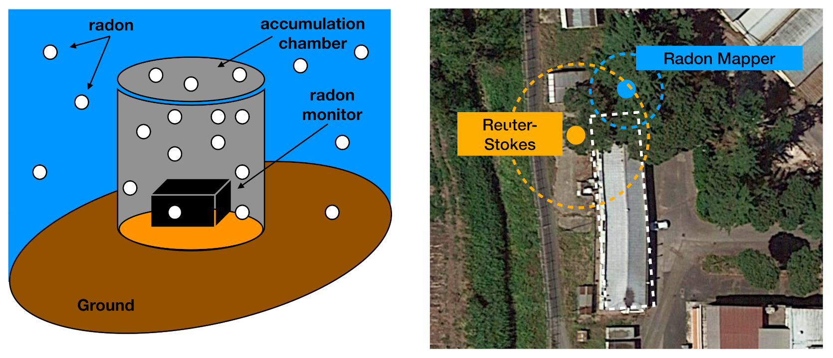
2.2. Radon Flux Monitor and External Accumulation Chamber

The RS sensitivity to the radon concentration variation was verified by comparing the dose rate data acquired by the RS with the radon concentration measured by a Radon Mapper detector placed in an external accumulation chamber installed near the RS detector. The accumulation chamber used was an iron half-barrel with a volume of 230 m${}^3$, completely closed, as shown in Figure 1. It was placed in a shaded spot in order to avoid a large temperature gradient between the inside and outside of the barrel during the day, which could greatly vary the radon exhalation flux.

Generally, the exhalation rate of Rn-220 (thoron) in soil is higher than the exhalation rate of radon [20], because the thorium concentration in the Earth crust is higher than that of U-238 (see the Discussion section for the site characteristics). The short half-life of thoron (56 s), however, prevents its diffusion on long distances, and the main part of the exhaled thoron decays directly in the soil without reaching the accumulation chamber. On the contrary, radon can be exhaled by the deeper layers of soil and reach the accumulation chamber thanks to its quite long half-life, making the net contribution of radon in the chamber greater than that of thoron [21]. In addition, the Radon Mapper monitor used within the accumulation chamber works in diffusion mode without any pumping, and has a limited sensitivity to thoron [22]. Considering these two points, it is possible to assume that the main contribution in the presented measurement is from radon, neglecting at first approximation the thoron contribution. The simultaneous measurements were conducted for 174 h (about seven days). The variation in the radon atom number over time inside the chamber is provided by the following differential equation [23]:

$$\dot{N}\left(t\right)=S^{\prime }-(\lambda +R)N\left(t\right)$$

(1)

where $\dot{N}\left(t\right)$ is the variation of radon atoms number in the accumulation chamber over time, $S^{\prime }$ is the number of radon atoms exhaled by the soil over time, $\lambda$ is the radon decay constant, and R is the leakage factor (which has the same dimensions of $\lambda$${\left[h\right]}^{-1}$). In the studied case the leakage factor is quite small, as it is due only to radon back-scattering in the soil. Dividing Equation (1) by the volume of the accumulation chamber and solving the differential equation between $t_0$ and $t>t_0$, the following expression is obtained:

$$C\left(t\right)=C_0{e}^{-(\lambda +R)t}+\frac{S_0}{\lambda +R}(1-e^{-(\lambda +R)t}).$$

(2)

where $C\left(t\right)$ and $C_0$ are the radon concentrations at time $\mathrm{t}$ and ${\mathrm{t}}_0$, respectively, and $S_0=S^{\prime }/V$ is the radon concentration exhaled by the soil, expressed as ${\left[\mathrm{Bq}\right]\left[\mathrm{m}\right]}^{-3}{\left[\mathrm{h}\right]}^{-1}$. The obtained equation can be used to fit the radon mapper data and extract the values of $S_0$ and R. The multiplication of the term $S_0$ by the accumulation chamber height (0.72 m) provides the parameter S, which is the radon flux exhaled by the soil, commonly measured as $\left[\mathrm{Bq}\right]{\left[\mathrm{m}\right]}^{-2}{\left[\mathrm{h}\right]}^{-1}$.

2.3. Meteorological Contributions to the Environmental Dose Rate—Model

Data acquired every 15 min by the RS detector were analyzed in order to investigate weather contributions, characterized by a timescale that spans from 30 min to several hours. The cross-sectional distribution of the dose rate data, the shape of which reflects the contribution of the radon concentration in the air, is generally studied in the literature using a log-normal model [4], because the variable is the product of multiple variables that, at first approximation, follow a Gaussian distribution. The log-normal function used to fit the cross-sectional distribution of dose rate data is given by the following formula [24]:

$$f\left(x\right)=\frac{1}{(x-\theta )\sigma \sqrt{2\pi }}{e}^{-\frac{{\left(ln\left(\frac{x-\theta }{m}\right)\right)}^2}{2{\sigma }^2}}$$

(3)

where $\sigma$ is the shape parameter (the standard deviation of the log of the distribution), $\theta$ is the location parameter, and m is the scale parameter (the median of the distribution). The data fitting procedure is based on ${\chi }^2$ minimization. The weather conditions of the days when the dose rate data fall in the distribution tails were investigated in order to determine correlations with specific meteorological events.

2.4. Retrospective Study to Investigate Seismic Contribution to the Dose Rate Time Series

The dose rate daily-averaged data collected by the Reuter–Stokes detector was used in this specific analysis because the timescale of the radon variations induced by seismic events was expected to be of few days order [5]. In addition, daily-averaged data are less sensitive to weather-induced variations; a dose rate peak due to the rain-out phenomenon and the following wash-out phase develops and ends in a few hours, and a 24-h average operation mitigates such contributions to the variable. A dedicated database was realized for this study, obtained by merging the daily-averaged dose rate data with the seismic event data (registered by the INGV seismographs network and free available on-line [25]) and the meteorological data collected by a weather station (Davis Vantage Pro 2 Plus Wireless [19]) placed a few hundred meters from the detector site.

Seismic events registered within a radius of 100 km from the detector and with a magnitude equal or higher than 3.5 on the Richter scale were selected according to [25] (see the discussion in the Results section). A total of eleven events were accordingly selected, and their locations are shown in Figure 2. During the considered period (2013–2018), a large number of seismic events were registered in central Italy, in particular in the Apennines region (see Figure 2); thus, a selection of events was needed in order to have the necessary degrees of freedom to correctly implement the model. For each of these eleven seismic events (in cases of multiple earthquakes in a single day, the one with the highest magnitude was chosen), a blind time region of eight days was defined in the daily dose rate time series, according to [5] (four days before the event, the day of the event, and three days following the event). After these regions were cut from the original time series, the remaining detached sub-series were used to study the dose rate values registered prior to the reference earthquakes. These series, indicated in the following as background series, include by definition the dose rate data registered concurrently with earthquakes with a magnitude less than 3.5 or located farther than 100 km from the detector in all kinds of weather conditions at the measurement site. The background series were analyzed using the Autoregressive Fractionally Integrated Moving Average (ARFIMA) class of models, a generalization of the conventional Autoregressive Integrated Moving Average (ARIMA) and the Autoeregressive Moving Average (ARMA) models. This class of models is particularly suitable for describing time series with long–memory, such as those analyzed in this work, which show auto-correlation functions with a decay-rate slower than exponential decay [26]. Considering a general variable at time t, $x_t$, a generalized form of the ARFIMA model can be written as

$$\varphi \left(L\right){(1-L)}^d{x}_t=\theta \left(L\right){ϵ}_t$$

(4)

where L is the lag operator, ${ϵ}_t$ is a white noise process, and $\varphi \left(L\right)$ and $\theta \left(L\right)$ are the p-order autoregressive (AR) and q-order moving average (MA) polynomials in L, respectively, with no common roots and all outside the unity circle. The fractional difference operator ${(1-L)}^d$, where $d\in (-0.5,0.5)$, is the part of the model which allows for the description of the long-term persistence of the time series, and is defined as

$${\displaystyle {(1-L)}^d=\sum _{k=0}^{\infty }\left(\genfrac{}{}{0pt}{}{d}{k}\right){(-L)}^k=\sum _{k=0}^{\infty }\frac{\Gamma (d+1)}{\Gamma (k+1)\Gamma (d+1-k)}{(-L)}^k}$$

(5)

The analysis of the dose rate time series was performed with the R package ARFIMA [27], which implements a frequency domain-based maximum likelihood estimation (MLE) of the fractional differentiation parameter d, the $\varphi \left(L\right)$ and $\theta \left(L\right)$ polynomials, and the noise variance ${\sigma }^2$. The best ARFIMA model for each background sub-series was evaluated using the Akaike Information Criterium (AIC) [26].

3. Results

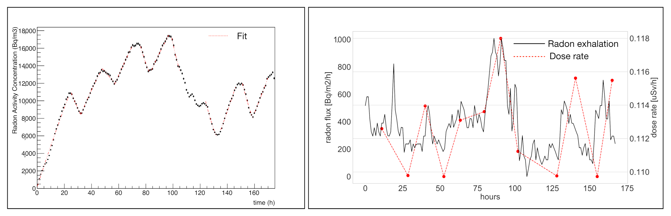
3.1. RS Sensitivity to the Radon Concentration Variations

Data acquired by the radon flux monitor during the 174 h of data-taking (almost seven days) along with the results of the fitting procedure according to Equation (2) are shown in Figure 3:

Data were fitted in time series intervals of about ten hours in both the increasing and the decreasing parts, in order to have sufficient degrees of freedom to obtain reliable results. In the fit procedure, the $\lambda$ parameter of Rn-222 is kept fixed while all the other parameters are free to vary. The radon exhalation flux, S, is calculated starting from the $S_0$ value (see Equation (2)) obtained in the fit, multiplying it for the height of the accumulation chamber (0.72 m). The result is then superimposed to the dose rate data registered simultaneously by the RS (see the right panel of Figure 3), using as time index the mean interval time considered in each fit.

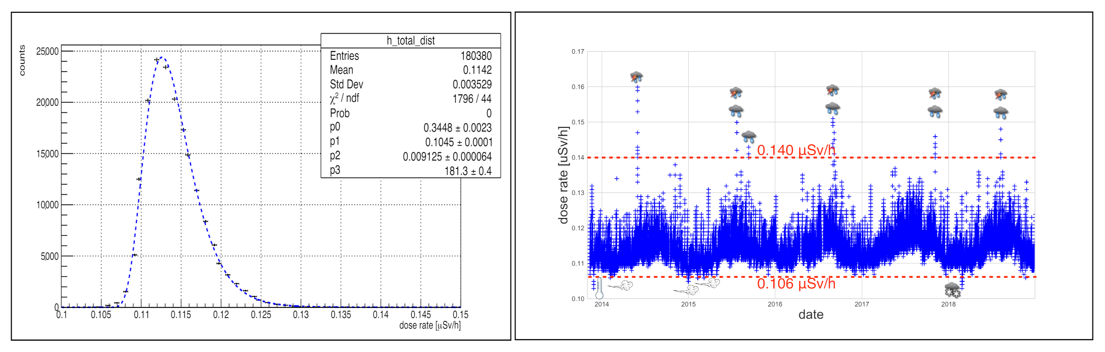
3.2. Weather Contribution

The cross-sectional distribution of the entire bulk of the data acquired over five years was fitted using the log-normal distribution in Equation (3). The results are shown in Figure 4.

The log-normal model explains the data distribution, even if large residuals (>5%) were observed along the distribution tails. In particular, these variations were noted below the value $S_L=0.106\mathsf{\mu }\mathrm{Sv}/\mathrm{h}$ and above the value $S_H=0.140\mathsf{\mu }\mathrm{Sv}/\mathrm{h}$. When dose rate values are characterized by large residuals, the meteorological conditions at the measurement site were investigated, finding some expected correlations; the results are summarized in

Table 1. Meteorological conditions at the measurement site for the days when dose rate registered values show large residual . The humidity values reported in the table are the average (first) and the maximum (in parenthesis). The last column reports where the dose rate data fall in the distribution, either in the low or high dose rate tail.

Date	Humidity (%)	Pressure (mbar)	Event	Dose Rate
27/11/2013	84 (93)%	1019	temperature <0	low tail
31/5/2014	78 (94)%	1013	storm, rain 20 mm	high tail
29/12/2014	47 (65)%	1014	gust, 61 km/h	low tail
9-10/2/2015	37 (65)%	1016	gust, 63 km/h	low tail
7/3/2015	38 (49)%	1016	gust, 54 km/h	low tail
24/7/2015	50 (74)%	1010	storm, rain 8 mm	high tail
31/8/2016	76 (94)%	1018	storm, rain 18 mm	high tail
16/9/2016	72 (94)%	1013	storm, rain 78 mm	high tail
5/11/2017	76 (93)%	1013	storm, rain 52 mm	high tail
26,28/2/2018	87 (100)%	1016	snow	low tail
8/8/2018	45 (65)%	1014	storm, rain 16 mm	high tail

.

3.3. Retrospective Study with ARFIMA Models

The daily-averaged gamma dose rate data ($\mathsf{\mu }\mathrm{Sv}/\mathrm{h}$), collected over five years beginning on 11 November 2013, at the ENEA Casaccia Research Center, are shown in Figure 5.

The time series of data acquired at the measurement site is characterized by an average background dose rate of $0.114\mathsf{\mu }\mathrm{Sv}/\mathrm{h}$, with a Standard Deviation of $0.003\mathsf{\mu }\mathrm{Sv}/\mathrm{h}$. Maximum values were registered in summer periods and minimum values in winter, for a maximum amplitude variation due to the seasonal cycle [6,7] of $0.006\mathsf{\mu }\mathrm{Sv}/\mathrm{h}$ within a semi-period of six months. In order to have sufficient degrees of freedom to implement the model, it was necessary to select significant events among the large number of seismic events registered in central Italy during these five years (see Figure 2). In a radius of 100 km from the detector, which corresponds to about three times the radius of the Earthquake Preparation Zone-EPZ [28], the maximum magnitude of expected earthquakes within it is between 4 and 5 [25].

For this reason, only events with a magnitude equal to or higher than 3.5 on the Richter scale were selected for the preliminary study, resulting in eleven events. Following [5], a blind time-region of eight days (four days before the event, the day of the seismic event, and three days after the event) was defined for each seismic event in the daily-averaged dose rate data series. Cutting these blind time regions from the original time series and considering two short detector-maintenance periods, a total of fourteen sub-series were defined to study the dose rate values before the reference seismic events.

Because the d fractional index value characterises the long-memory of the entire dose rate time series, a first round of fits on the sub-series was performed. All of the estimated d values consistently converged to 0.11, in particular for the longest sub-series, as this is a characteristic of stationary time series ($d<1$).

A second fitting procedure was performed on the sub-series by keeping fixed the d parameter with the weighted average of the values obtained before ($0.11\pm 0.04$) and defining the parameters of the best ARFIMA model for each sub-series according to the Akaike Information Criterion. The results are shown in Figure 6.

Table 2. Details of the ARFIMA best model evaluated for each sub-series. The last two columns report the order of the AutoRegressive (AR) and Moving Average (MA) polynomials.

Sub-Series Number	Total Length (Days)	Background Length (Days)	AR	MA
1	22	14	7	0
2	312	312	2	1
3	597	589	8	5
4	20	20	0	0
5	456	456	5	4
6	131	123	5	2
7	30	22	1	0
8	34	26	0	2
9	17	9	6	0
10	21	13	8	0
11	11	3	0	0
12	109	101	1	2
13	21	13	8	1
14	73	65	1	0

reports the details of the best ARFIMA models used to fit each subseries selected in this work to forecast the expected dose rate values in the defined blind regions.

Comparing the ARFIMA forecasting and the real data in the blind regions, significant deviations (>2$\sigma )$ are observed. Such deviations (called anomalies in the following) can be positive, with a measured gamma background higher than the expected value (as reported in literature for earthquake gaseous precursors [5]), or negative, with a gamma background lower than the expected value. The method used for this analysis was further validated on ten mock subseries extracted from a time period between September 2017 and December 2018 when no seismic events with magnitude higher than 3.5 and closer than $100\mathrm{km}$ were registered (background conditions); no anomalies were found (see Discussion section). Before discussing the potential relationship between the observed anomalies and seismic events, it is important to consider other contributors that can induce variations in the time series in order to rule out any potential interference. These are examined in the following:

• Rainstorms and Snow—these types of weather events are quite uncommon at the measurement site. Specifically, rainstorm and snow as individuated in the weather contribution study do not occur in the defined blind regions of the examined sub-series. The correlation between the daily-averaged dose rate and rain data was investigated and no significant (p-$\mathrm{value}=0.866$) correlation ($\rho =-0.005$) was found. The lack of an evident correlation with rain can be explained by the daily averaging operation on the dose rate data, which mitigates the presence of outliers due to the rain-out and wash-out phenomena [4], as these are characterized by hourly timescale.
• Radon Annual Cycle—This phenomenon manifests itself on a monthly timescale, inducing variations of less than $1\%$ on a month at the measurement site (see Figure 5). The blind regions defined for the studied sub-series are of eight days, where this effect is negligible. Moreover, the ARFIMA models used in this part of the work allow the consideration of long-persistence in the time series, in this case due to the radon annual cycle contribution.
• Radon Daily Cycle—The radon daily cycle contribution is due to atmospheric mixing categories [29] and manifests itself on hourly timescale as a day/night time effect. Averaging the dose rate on a daily basis mitigates the impact of any effects on the data, in the same way as for the rain case.
• Anthropogenic Radionuclide Contributions—As the detector is located within a Research site which hosts several radiological and nuclear installations (including two research nuclear reactors), the contributions of anthropogenic radionuclides eventually released into the environment was examined. Anthropogenic radionuclides releases due to either accidental or normal activities were investigated by checking the measurements performed by the safety environmental measurement network of the ENEA site. This network consists of a series of dosimeters, detectors, and periodical contamination measurements on environmental samples (i.e., water, grass, soil, milk, air) taken in an area covering a radius of 5 km from the ENEA Research Center. During the time period considered in this study, there was no evidence of any release of anthropogenic radionuclides; therefore, such a contribution can be excluded.
• Other Effects—The correlation of the dose rate daily averaged data with other weather variables, such as pressure, temperature and humidity, was considered. In the study, high significance (p-$\mathrm{value}=1.1\times {10}^{-22}$ and p-$\mathrm{value}=2.8\times {10}^{-8}$), though weak anti-correlations, were found for relative humidity ($\rho =-0.265$) and pressure ($\rho =-0.152$). On the other hand, the dose rate daily averaged data were significantly (p-$\mathrm{value}=2.4\times {10}^{-22}$) correlated with the temperature ($\rho =0.726$). Even if the correlation between temperature, pressure and daily dose rate is due to a well known effect of these exogenous variables on the daily radon cycle [30], sudden changes in temperature, and to a lesser extent, in pressure and relative humidity, can generate variations that can mimic those generated by seismic events. For this reason, the rain, relative humidityextent, pressure, and temperature time series are considered in following discussion of the results obtained by the ARFIMA modelextents.

In light of the above considerations, the potential interference to the daily average dose rate variations can be excluded. Therefore, the possible relationship with seismic events can be considered. In particular, in the next section the three cases with the highest number of consecutive days when the anomalies were registered are described and discussed in detail.

4. Discussion

4.1. RS Sensitivity to the Radon Concentration Variations

The results shown in Figure 3 confirm the detector’s sensitivity to the radon activity concentration in the air, as can be seen from the superimposition of the radon exhalation flux and the dose rate data time series. The mathematical model (Equation (2)) assumes that the radon exhalation flux is constant for the time interval considered for the fitting procedure. The evaluated high-exhalation radon fluxes are consistent with the volcanic origin of the soil type at the measurement site. According to the Geochemical Atlas of Europe FOREGS , the Uranium and Thorium concentrations for the measurement site are among the highest values found in Europe [31].

The large Ra-226 activity concentration reported in

Table 3. Uranium and Thorium soil content profile according to FOREGS data.

Soil Sample Depth	Th (mg/kg)	U (mg/kg)	Ra-226 (Bq/kg)
0–10 cm	23.1	6.60	81.5
10–25 cm	24.0	7.37	91.0

, evaluated by multiplying the U concentration by a factor equal to 12.35, according to [32], can account for the high radon fluxes observed [33,34]. The assumption made on the constant exhalation rate in the time interval used for the fit can be therefore considered valid, demonstrating with this measure the sensitivity of the RS to dose-rate variation induced by radon and its gamma emitting progeny in air.

However, it must be considered that even if the data are acquired hourly, the fitting procedure fixes the time interval to evaluate radon exhalation at about 10 h, limiting the opportunity to examine in detail the radon day/night cycle induced by the atmospheric mixing categories [29]. It would be interesting to include this kind of study in future investigations.

4.2. Weather Contribution

The log-normal model (Equation (3)) used to study the cross-sectional distribution of the dose rate data acquired every 15 min highlights certain peculiar influences of the weather on the dose rate time series. In particular dose rate values falling in the high dose rate tail of the distribution were correlated with storms and abundant precipitation according to the observation of the rain-out phenomenon. The dose rate values falling in the low dose rate tail of the distribution appear to be correlated with strong wind and snow. For this last event, the wash-out phenomenon is easily observable, as it lasts for few days until the snow melts. The weather events highlighted by the presented method are quite unlikely at the measurement site; precipitation of only a few mm of rain, soft winds, and temperatures well above $0{}^{\circ }C$ are the general conditions characterizing the CR Casaccia site.

4.3. Retrospective Study with ARFIMA Models

Eleven earthquakes registered in 2013–2017 were identified by applying the selection criteria to seismic events, mostly located in the N-N-E direction at a distance between 75 and 100 km (see

Table 4. Seismic events related to environmental gamma anomalies detected at the Casaccia Research Center site. Those events where anomalies persisted for the longest time period (in days) are reported in bold font. The distance from the detector was calculated using the Haversine formula.

Location	Distance (km)	Earthquake Date	Magnitude	Deviations (Number of Days)	Hypocenter Depth (km)
Cittareale (RI)	99	30/11/2013	3.7	7	10
Castel San Giorgio (TR)	78	30/05/2016	4.1	1	8
Cittareale (RI)	99	30/10/2016	4.0	1	11
Capitignano (AQ)	97	29/11/2016	4.4	4	11
Campello sul Clitunno (PG)	92	02/01/2017	3.9	2	8
Montereale (AQ)	97	18/01/2017	4.2	7	11
Spoleto (PG)	76	09/02/2017	3.7	4	8
Montereale (AQ)	97	20/02/2017	3.9	2	11
Pizzoli (AQ)	98	09/06/2017	3.8	0	12
Cittareale (RI)	99	30/06/2017	3.8	6	12
S. Marsicana (AQ)	85	10/09/2017	3.7	3	8

). No weather events reported in Table 2 fall within the considered blind regions.

The earthquake cases for which dose rate anomalies persisted for the longest time period (in days) are reported with bold font in Table 4 and are detailed in the following. A separate discussion should be provided for the earthquake registered in Cittareale in 2013; however, even if there are significant deviations in the data, there is a lack of meteorological data for that period. Hence, it is not considered in the following discussion.

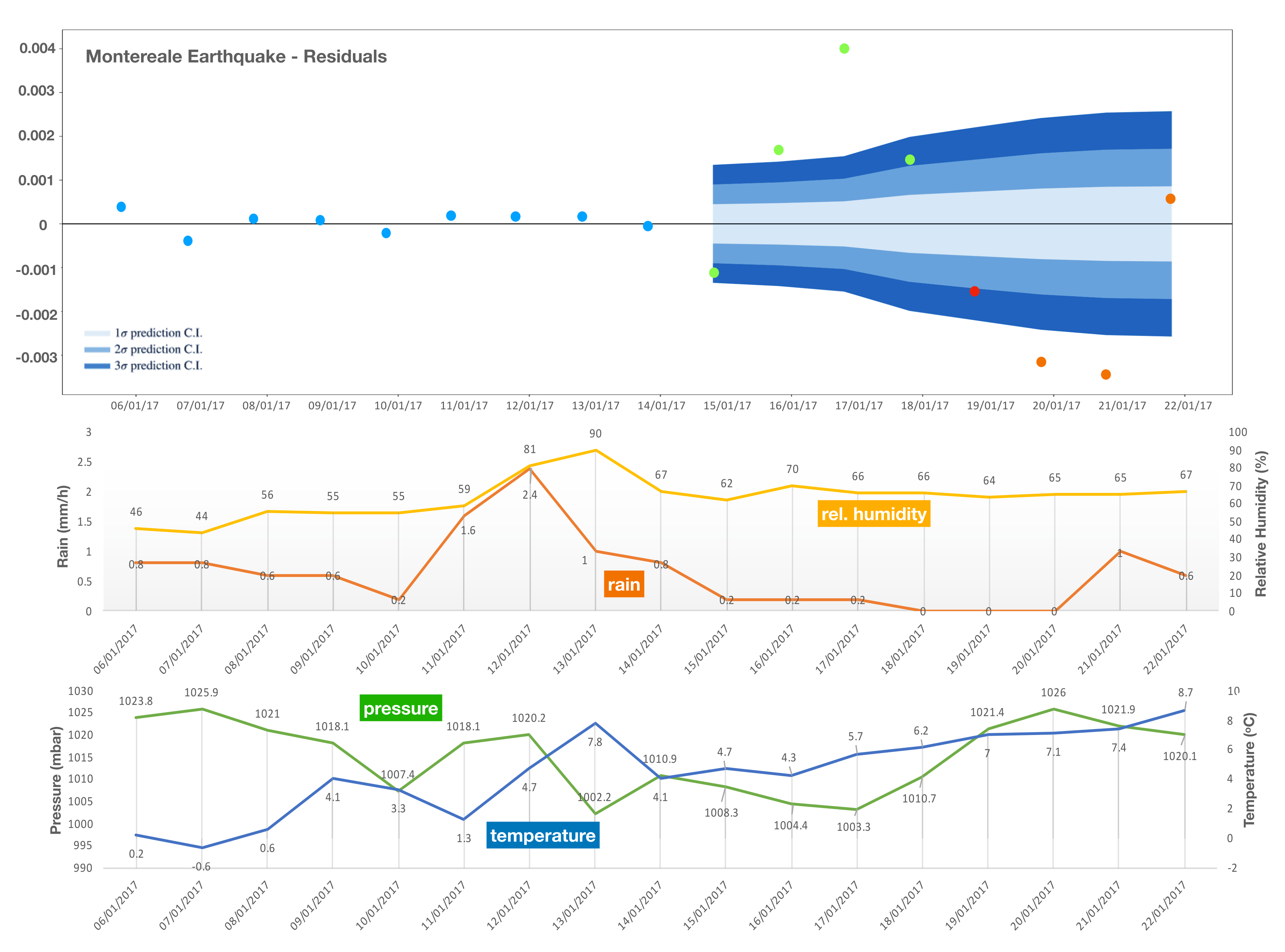
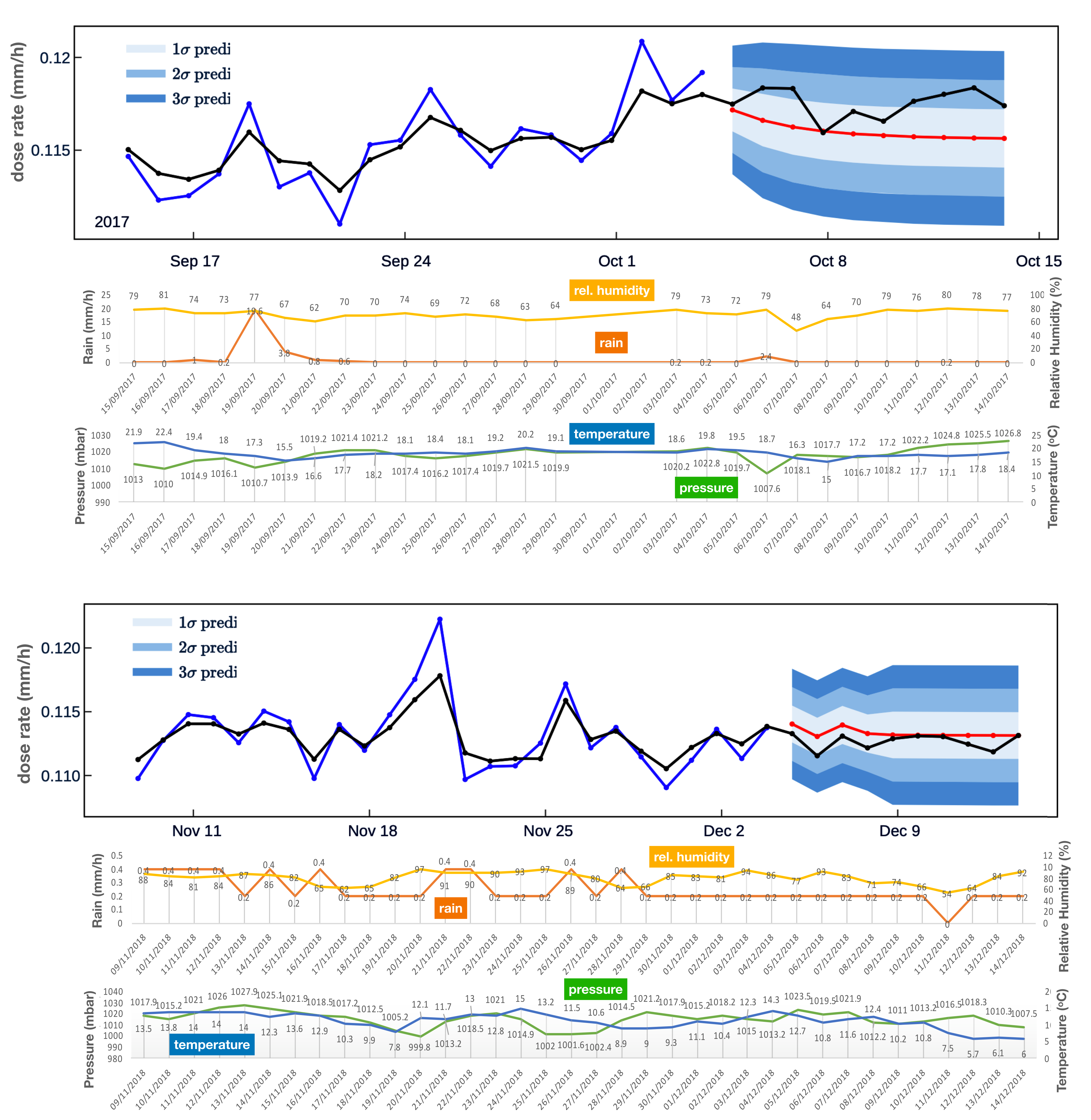
• Montereale earthquake—18-01-2017: The earthquake epicenter (magnitude 4.2) was located at 42.58 (lat), 12.23 (lon), 97 km from the detector. The hypocenter was located 8 km underground. In the blind time-region, seven outliers (deviations $>2\sigma$), four before the earthquake, one during the earthquake day, and two after the event, were identified.

  Figure 7. Montereale earthquake (color on-line)—upper panel: residuals of the best ARFIMA model. Blue points correspond to the dose rate background data and green points to the pre-shock events; the red point is the earthquake event and the orange points represent aftershock events. The confidence level bands for coverage factor k = 1, 2, 3 (from the lightest to the darkest blue) are drawn in the blind time region. In the middle and lower panels the relative humidity, rainfall, temperature, and pressure time series are shown, as indicated by the respective labels.

  Figure 7. Montereale earthquake (color on-line)—upper panel: residuals of the best ARFIMA model. Blue points correspond to the dose rate background data and green points to the pre-shock events; the red point is the earthquake event and the orange points represent aftershock events. The confidence level bands for coverage factor k = 1, 2, 3 (from the lightest to the darkest blue) are drawn in the blind time region. In the middle and lower panels the relative humidity, rainfall, temperature, and pressure time series are shown, as indicated by the respective labels.
  Residuals, rain, temperature, pressure and humidity data are shown in Figure 7. Positive anomalies (dose rate higher than the one predicted by the model) and negative ones (dose rate lower than the one predicted by the model) were identified in the blind time region. Small changes in weather conditions were registered over three days of background data (from 11 to 13 January) due to rainfall. The model, however, correctly follows the data behaviour, as shown by the residuals. No sudden changes in weather data were registered within the blind time region; the occurred minor changes in rain data in the background period, that can potentially induce variations, are correctly considered in the model, as it is shown by the residual distribution.

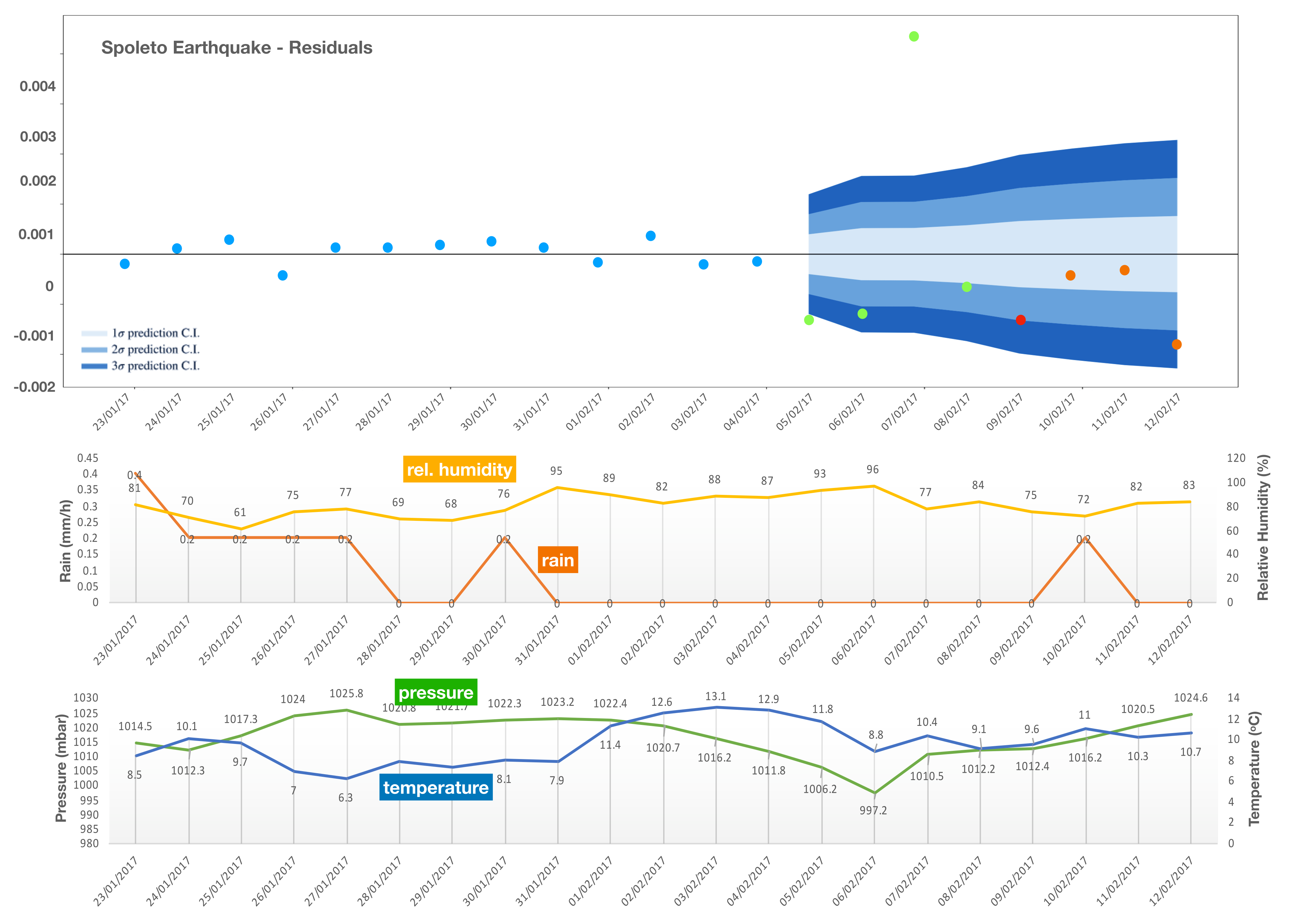
• Spoleto—09-02-2017: The earthquake epicenter (magnitude 3.7) was located at 42.66 (lat), 12.68 (lon), 76 km from the detector. The hypocenter was located 8 km underground. In the blind time-region, four outliers (deviations $>2\sigma$), three before the earthquake and one after the seismic event, were identified. Residuals, rain, temperature, pressure and humidity data are shown in Figure 8. Positive and negative anomalies were identified in the blind time region. No sudden changes in weather conditions were registered for that period, in particular for days when anomalies were identified.

  Figure 8. Spoleto earthquake (color on-line)—upper panel: residuals of the best ARFIMA model. Blue points correspond to the dose rate background data and green points to the pre-shock events; the red point is the earthquake event and the orange points represent aftershock events. The confidence level bands for coverage factor k = 1, 2, 3 (from the lightest to the darkest blue) are drawn in the blind time region. In the middle and lower panels the relative humidity, rainfall, temperature, and pressure time series are shown, as indicated by the respective labels.

  Figure 8. Spoleto earthquake (color on-line)—upper panel: residuals of the best ARFIMA model. Blue points correspond to the dose rate background data and green points to the pre-shock events; the red point is the earthquake event and the orange points represent aftershock events. The confidence level bands for coverage factor k = 1, 2, 3 (from the lightest to the darkest blue) are drawn in the blind time region. In the middle and lower panels the relative humidity, rainfall, temperature, and pressure time series are shown, as indicated by the respective labels.

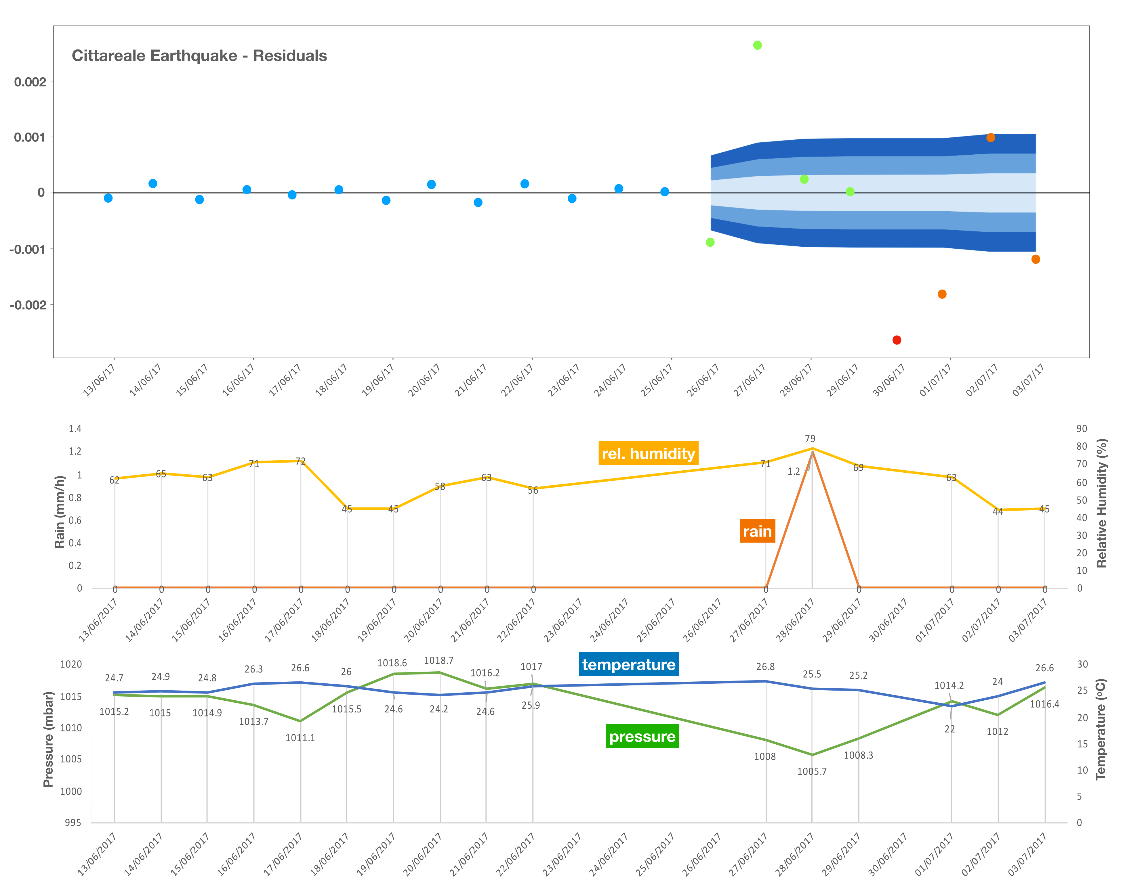
• Cittareale earthquake—30-06-2017: The earthquake epicenter (magnitude 3.6) was located at 42.63 (lat), 12.68 (lon), 99 km from the detector. The hypocenter was located 12 km underground. In the blind time-region defined for this earthquake, six outliers, two before the earthquake, one during the seismic event, and three after the earthquake, were identified. Residuals, rain, temperature, pressure and humidity data are shown in Figure 9. Positive and negative anomalies were identified . There is a lack of meteorological data from 23 June to 26 June as well as on 30 June. For the days from 23 June to 25 June, the model correctly follows the background data behaviour. For 25 and 30 June, sudden changes in the weather variables can be excluded because the points that follow the missing data do not highlight any anomaly in the previous days (e.g., in the event of a strong rainfall, changes in pressure and temperature should be observed in the day after along with a peak in relative humidity with a lag of approximately one day). Moreover, considering the climate conditions of the detector site region, a sudden change in these parameters is quite unlikely.

  Figure 9. Cittareale earthquake (color on-line)—upper panel: residuals of the model. Blue points correspond to the dose rate background data and green points to the pre-shock events; the red point is the earthquake event and the orange points represent aftershock events. The confidence level bands for coverage factor k = 1, 2, 3 (from the lightest to the darkest blue) are drawn in the blind time region. In the middle and lower panels the relative humidity, rainfall, temperature, and pressure time series are shown, as indicated by the respective labels.

  Figure 9. Cittareale earthquake (color on-line)—upper panel: residuals of the model. Blue points correspond to the dose rate background data and green points to the pre-shock events; the red point is the earthquake event and the orange points represent aftershock events. The confidence level bands for coverage factor k = 1, 2, 3 (from the lightest to the darkest blue) are drawn in the blind time region. In the middle and lower panels the relative humidity, rainfall, temperature, and pressure time series are shown, as indicated by the respective labels.

The eleven earthquakes considered in this work were all superficial seismic events (hypocenter between 0 and 70 km) located within 100 km of the detector. The dose rate data acquired during other earthquakes with a magnitude less than 3.5 or with an epicenter more distant than 100 km were considered as background in the ARFIMA model training. Analysis of the mock-subseries used to test false positive results, shows no evidences of deviations beyond 2$\sigma$. Two typical results obtained via the mock subseries are shown in Figure 10.

5. Conclusions

This work presents the results of a study on the environmental gamma dose rate variations induced by natural effects, in particular weather and seismic events. By exploiting the different timescales of variations induced by different types of phenomena it is possible to discriminate their origin and apply suitable analysis techniques, allowing for the study of their characteristics.

The comparative measurements simultaneously performed by the Reuter–Stokes and the Radon Mapper detector confirmed our hypothesis that the ionization chamber is sensitive to variations in concentrations of radon and its gamma emitting progeny in the air. In the future, it would be desirable to perform simultaneous measurements using other techniques, such as an external accumulation chamber with forced ventilation that is activated at preset times [23]. The filling and subsequent ventilation allows radon to accumulate in the chamber only during the first hours, when the concentration rises. Using this approach, a simple linear model can be applied to infer the radon exhalation flux (see Equation (1)). This technique allows for a finer time grid in terms of radon flux measurements, opening up the opportunity to investigate the radon daily cycle in more detail.

The study performed using a log-normal model of the cross-sectional distribution of dose-rate data taken every 15 minutes, highlighted uncommon weather conditions at the measurement site, finding correlations with rainfalls (rain-out and wash-out phenomena), snow, and wind. Concerning the last part of the work, all of the results obtained in the analysis were used to rule out those phenomena that can mimic dose-rate variations induced by seismic events. The study represents a first step in implementing the ARFIMA class of model to investigate dose rate time series; although further studies remain necessary in order to establish a solid correlation between dose rate anomalies and seismic events, preliminary considerations can be reached. Anomalies in dose rate data that could be interpreted as seismic precursors were identified in seven out of eleven studied earthquakes, and for five of these the anomalies began four days earlier than the earthquake. The observed deviations have a sign that can be also negative (only positive deviations are reported in the literature [4]), a phenomenon that can be explained by the displacement of the radon release region far from the detector due to changes in the underground gas pattern caused by seismic events. Another interesting result is related to the best ARFIMA models obtained in this study; the order of the auto-regressive (AR) part is considerably higher than the moving average (MA) part, probably representing a characteristic of the gamma environmental dose rate variable (see Table 2). Further studies are currently in progress to improve the method presented in this work, which constitutes only a first investigation into its potential application for studying anomalies in radon variations. The first concern is the implementation of other models to identify possible deviations in the dose rate time series, such as ARFIMAX, which allows the inclusion of exogenous variables such as the weather parameter [35], and CARFIMA (Continuos ARFIMA), which allows forecast periods with no data to be overcome [36]), as well as unsupervised algorithms to identify deviations, such as the Isolation Forest algorithm [37]. The results obtained by these different methods can then be compared in order to check the consistency of the findings. Another important improvement for investigating the possibility of correlating a specific earthquake with the dose rate data variations is the planned installation of two other RS detectors, each with a dedicated weather station nearby. These detectors will be placed about 100 km from the Casaccia site and 100 km apart from each other, allowing to explore the applicability of a triangulation technique based on the EPZ empirical formula .

References

1. Saito, K.; Ishigure, N.; Petoussi-Henss, N.; Schlattl, H. Effective dose conversion coefficients for radionuclides exponentially distributed in the ground. Radiat. Environ. Biophys. 2012, 51, 411–423. [Google Scholar] [CrossRef] [PubMed] [Green Version]
2. Čeliković, I.; Pantelić, G.; Vukanac, I.; Krneta Nikolić, J.; Živanović, M.; Cinelli, G.; Gruber, V.; Baumann, S.; Quindos Poncela, L.S.; Rabago, D. Outdoor Radon as a Tool to Estimate Radon Priority Areas—A Literature Overview. Int. J. Environ. Res. Public Health 2022, 19, 662. [Google Scholar] [CrossRef] [PubMed]
3. Tchorz-Trzeciakiewicz, D.E.; Rysiukiewicz, M.T. Ambient gamma dose rate as an indicator of geogenic radon potential. Sci. Total Environ. 2021, 755, 142771. [Google Scholar] [CrossRef] [PubMed]
4. Burnett, J.L.; Croudace, I.W.; Warwick, P.E. Short-lived variations in the background gamma-radiation dose. J. Radiol. Prot. 2007, 7, 525–533. [Google Scholar] [CrossRef]
5. Immé, G.; Morelli, D. Radon as earthquake precursor. In Earthquake Research and Analysis; D’Amico, S., Ed.; IntechOpen: Rijeka, Croatia, 2012; Chapter 7. [Google Scholar] [CrossRef] [Green Version]
6. Melintescu, A.; Chambers, S.D.; Crawford, J.; Williams, A.G.; Zorila, B.; Galeriu, D. Radon-222 related influence on ambient gamma dose. Pure Appl. Geophys. 2018, 189, 67–68. [Google Scholar] [CrossRef]
7. Inomata, Y.; Chiba, M.; Igarashi, Y.; Aoyama, M.; Hirose, K. Seasonal and spatial variations of enhanced gamma ray dose rates derived from 222Rn progeny during precipitation in Japan. Atmos. Environ. 2007, 41, 8043–8057. [Google Scholar] [CrossRef]
8. Greenfield, M.B.; Domondon, A.T.; Okamoto, N.; Watanabe, I. Variation in γ-ray count rates as a monitor of precipitation rates, radon concentrations, and tectonic activity. J. Appl. Phys. 2002, 91, 1628–1633. [Google Scholar] [CrossRef]
9. RSS -131- ER / RSS -131 User’s Manual—Part Number: RSS-131-OM Revision: R. 2014. Available online: https://www.industrial.ai/sites/g/files/cozyhq596/files/acquiadam_assets/rss_131_user_manual_all_units_rev_r_english.pdf (accessed on 28 March 2022).
10. Takeuchi, N.; Katase, A. Rainout-Washout Model for Variation of Environmental Gamma-Ray Intensity by Precipitation. J. Nucl. Sci. Technol. 1982, 19, 393–409. [Google Scholar] [CrossRef]
11. Burnett, J.L. Understanding the Contribution of Naturally Occurring Radionuclides to the Measured Radioactivity in AWE Environmental Samples. Ph.D. Thesis, University of Southampton, Southampton, UK, 2007. [Google Scholar]
12. Tsvetkova, T.; Monnin, M.; Nevinsky, I.; Perelygin, V. Research on variation of radon and gamma-background as a prediction of earthquakes in the caucasus. Radiat. Meas. 2001, 33, 1–5. [Google Scholar] [CrossRef]
13. Fu, C.; Wang, P.; Lee, L.; Lin, C.; Chang, W.; Giuliani, G.; Ouzounov, D. Temporal variation of gamma rays as a possible precursor of earthquake in the longitudinal valley of eastern taiwan. J. Asian Earth Sci. 2015, 114, 362–372. [Google Scholar] [CrossRef]
14. Barbosa, S.; Miranda, P.; Azevedo, E.B. Short-term variability of gamma radiation at the arm eastern north atlantic facility (azores). J. Environ. Radioact. 2017, 172, 218–231. [Google Scholar] [CrossRef] [PubMed] [Green Version]
15. Beran, J. Fundamentals of Earthquake Prediction; John Wiley and Sons: New York, NY, USA, 1994. [Google Scholar]
16. Ianakiev, K.D.; Alexandrov, B.S.; Littlewood, P.B.; Browne, M.C. Temperature behavior of NaI (Tl) scintillation detectors. Nucl. Instrum. Methods Phys. Res. Sect. 2006, 607, 432–438. [Google Scholar] [CrossRef] [Green Version]
17. Tsvetkova, T.; Nevinsky, I.; Nevinsky, V. Results of spectral monitoring of environmental gamma background in a fault zone of the western caucasus for seismological application. J. Environ. Radioact. 2014, 69, 35–49. [Google Scholar] [CrossRef]
18. Bollettino Sismico Italiano—Istituto Nazionale di Geofisica e Vulcanologia. Available online: http://terremoti.ingv.it/ (accessed on 10 November 2021).
19. Meteonenetwork Weater Station. Available online: http://my.meteonetwork.it/station/laz198 (accessed on 10 November 2021).
20. Hosoda, M.; Michikuni, S.; Masato, S.; Yuji, Y.; Masahiro, F. Radon and Thoron Exhalation Rates and Their Some Correlating Factors. Available online: https://www.ipen.br/biblioteca/cd/irpa/2004/files/6a30.pdf (accessed on 10 May 2022).
21. Gulshan, K.; Kumari, P.; Kumar, A.; Prasher, S.; Kumar, M. A study of radon and thoron concentration in the soil along the active fault of NW Himalayas in India. Ann. Geophys. 2017, 60, S0329. [Google Scholar]
22. Omori, Y.; Shimo, M.; Janik, M.; Ishikawa, T.; Yonehara, H. Variable Strength in Thoron Interference for a Diffusion-Type Radon Monitor Depending on Ventilation of the Outer Air. Int. J. Environ. Res. Public Health 2020, 17, 974. [Google Scholar] [CrossRef] [PubMed] [Green Version]
23. Rábago, D.; Quindós, L.; Vargas, A.; Sainz, C.; Radulescu, I.; Ioan, M.R.; Cardellini, F.; Capogni, M.; Rizzo, A.; Celaya, S.; et al. Intercomparison of Radon Flux Monitors at Low and at High Radium Content Areas under Field Conditions. Int. J. Environ. Res. Public Health 2022, 19, 4213. [Google Scholar] [CrossRef] [PubMed]
24. NIST/SEMATECH e-Handbook of Statistical Methods. Available online: https://www.itl.nist.gov/div898/handbook/eda/section3/eda3669.htm (accessed on 30 March 2022).
25. Sundar De, S. Seismo-Electromagnetism: Atmosphere-Lithosphere Coupling. Available online: https://www.researchgate.net/publication/324756915_Seismo-Electromagnetism_Atmosphere-Lithosphere_coupling/link/5ae0a0d8a6fdcc91399dcf26/download (accessed on 1 March 2022).
26. Beran, J. Statistics for Long-Memory Processes; CRC Press: Boca Raton, FL, USA, 1994. [Google Scholar]
27. Veenstra, J.Q.; McLeod, A.I. Fractional ARIMA (and Other Long Memory) Time Series Modeling. Available online: https://cran.r-project.org/web/packages/ARFIMA/ARFIMA.pdf (accessed on 29 November 2020).
28. Dobrovolsky, I.P.; Zubkov, S.I.; Miachkin, V.I. Estimation of the size of earthquake preparation zones. Pure Appl. Geophys. 1979, 117, 1025–1044. [Google Scholar] [CrossRef]
29. Grossi, C.; Vogel, F.R.; Curcoll, R.; Àgueda, A.; Vargas, A.; Rodó, X.; Morguí, J.-A. Study of the daily and seasonal atmospheric CH4 mixing ratio variability in a rural Spanish region using 222Rn tracer. Atmos. Chem. Phys. 2018, 18, 5847–5860. [Google Scholar] [CrossRef] [Green Version]
30. Siino, M.; Scudero, S.; Cannelli, V.; Piersanti, A.; D’Alessandro, A. Multiple seasonality in soil radon time series. Sci. Rep. 2019, 1, 8610. [Google Scholar] [CrossRef] [Green Version]
31. FOREGS Geochemical Atlas of Europe—Part 1: Background Information, Methodology and Maps. Available online: http://weppi.gtk.fi/publ/foregsatlas/maps_table.php (accessed on 11 May 2022).
32. Joel, E.S.; Omeje, M.; Olawole, O.C.; Adeyemi, G.A.; Akinpelu, A.; Embong, Z.; Saeed, M.A. In-situ assessment of natural terrestrial-radioactivity from Uranium-238 (238U), Thorium-232 (232Th) and Potassium-40 (40K) in coastal urban-environment and its possible health implications. Sci. Rep. 2021, 11, 17555. [Google Scholar] [CrossRef]
33. Ashry, A.H.; Arafa, W.; Abou-Leila, M.; Taha, A.A.; AbdElnaeem, O.E. Radium Content and Radon Exhalation Rate from Natural Samples Using SSNTD. J. Radiat. Nucl. Appl. 2019, 4, 101–107. [Google Scholar]
34. Porstendoerfer, J.; Butterweck, G.; Reineking, A. Daily variation of the radon concentration indoors and outdoors and the influence of meteorological parameters. Health Phys. 1994, 67, 283–287. [Google Scholar] [CrossRef]
35. Degiannakis, S. ARFIMAX and ARFIMAX-TARCH realized volatility modeling. J. Appl. Stat. 2008, 35, 1169–1180. [Google Scholar] [CrossRef]
36. Tsai, H. On continuous-time autoregressive fractionally integrated moving average processes. Bernoulli 2009, 15, 178–194. [Google Scholar] [CrossRef]
37. Liu, F.T.; Ting, K.M.; Zhou, Z.H. Isolation Forest. Available online: https://cs.nju.edu.cn/zhouzh/zhouzh.files/publication/icdm08b.pdf?q=isolation-forest (accessed on 29 March 2022).
Figure 1. (Left) A sketch of the Radon Mapper experimental setup with the accumulation chamber. (Right) Aerial view of the measurement site with the position of the Reuter–Stokes and the Radon Mapper.
Environments 09 00066 g001
Figure 2. Distribution of seismic events around the RS detector. The Z axis represents the number of events, and the black points are the seismic events chosen to test the analysis method (Credits: Google My Maps).
Environments 09 00066 g002
Figure 3. (Left) Radon activity concentration in the accumulation chamber (black dots) with the fit results superimposed (red dashed line, color on-line). (Right) Superimposition of the radon exhalation flux (red dashed line, color on-line) evaluated using fit results and the simultaneous dose rate measurement results obtained by the Reuter–Stokes (black continuous line).
Environments 09 00066 g003
Figure 4. (Left) Cross sectional distribution of the dose rate data acquired every 15 min and the log-normal fit (blue dashed line, color on-line). (Right) dose rate time-series showing the meteorological events that are the source of the variations.
Environments 09 00066 g004
Figure 5. Daily averaged dose rate ( μ Sv / h ) measured from November 2013 to December 2018, for a total of 2702 collected daily values.
Environments 09 00066 g005
Figure 6. Results of the ARFIMA model forecasting in the blind time-regions defined around the seismic events of interest (color on-line). The solid black line represents the daily averaged dose rate data, the blue line corresponds to the fit results using the ARFIMA model, and the red line is the ARFIMA prediction in the blind time region. For the blind time regions, the confidence level bands for coverage factor k = 1, 2, 3 (from the lightest to the darkest blue, color on-line) are drawn. Solid (empty) green markers represent data before the earthquake that deviate more (less) than 2 σ from the prediction. The red solid circle represents the earthquake event and the solid (empty) orange markers represent data after the earthquake that deviate more (less) than 2 σ from the prediction. The time series for the seismic event registered on 20 February 2017 is not reported in the figure because the background series was too brief (three days) to build a reliable ARFIMA model.
Environments 09 00066 g006
Figure 10. Typical results obtained for sub-series extracted from a long background-only series (color on-line). The first and third panels show the model results for two different data series. The black lines represent the collected dose rate data (daily average), the blue lines correspond to the the fits of the best ARFIMA models, and the red lines correspond to the model predictions. The confidence level bands for coverage factor k = 1, 2, 3 (from the lightest to the darkest blue) are drawn in the validation region. In the second and fourth panels the relative humidity, rainfall, temperature, and pressure time series are shown, as indicated by the respective labels.
Environments 09 00066 g010