Comparison of UAV LiDAR and Digital Aerial Photogrammetry Point Clouds for Estimating Forest Structural Attributes in Subtropical Planted Forests

Abstract

Estimating forest structural attributes of planted forests plays a key role in managing forest resources, monitoring carbon stocks, and mitigating climate change. High-resolution and low-cost remote-sensing data are increasingly available to measure three-dimensional (3D) canopy structure and model forest structural attributes. In this study, we compared two suites of point cloud metrics and the accuracies of predictive models of forest structural attributes using unmanned aerial vehicle (UAV) light detection and ranging (LiDAR) and digital aerial photogrammetry (DAP) data, in a subtropical coastal planted forest of East China. A comparison between UAV-LiDAR and UAV-DAP metrics was performed across plots among different tree species, heights, and stem densities. The results showed that a higher similarity between the UAV-LiDAR and UAV-DAP metrics appeared in the dawn redwood plots with greater height and lower stem density. The comparison between the UAV-LiDAR and DAP metrics showed that the metrics of the upper percentiles (r for dawn redwood = 0.95–0.96, poplar = 0.94–0.95) showed a stronger correlation than the lower percentiles (r = 0.92–0.93, 0.90–0.92), whereas the metrics of upper canopy return density (r = 0.21–0.24, 0.14–0.15) showed a weaker correlation than those of lower canopy return density (r = 0.32–0.68, 0.31–0.52). The Weibull α parameter indicated a higher correlation (r = 0.70–0.72) than that of the Weibull β parameter (r = 0.07–0.60) for both dawn redwood and poplar plots. The accuracies of UAV-LiDAR (adjusted (Adj)R² = 0.58–0.91, relative root-mean-square error (rRMSE) = 9.03%–24.29%) predicted forest structural attributes were higher than UAV-DAP (Adj-R² = 0.52–0.83, rRMSE = 12.20%–25.84%). In addition, by comparing the forest structural attributes between UAV-LiDAR and UAV-DAP predictive models, the greatest difference was found for volume (ΔAdj-R² = 0.09, ΔrRMSE = 4.20%), whereas the lowest difference was for basal area (ΔAdj-R² = 0.03, ΔrRMSE = 0.86%). This study proved that the UAV-DAP data are useful and comparable to LiDAR for forest inventory and sustainable forest management in planted forests, by providing accurate estimations of forest structural attributes.

1. Introduction

Planted forests cover approximately 7.3% (290 million ha) of global forests, and they increased steadily by over 105 million ha since the 1990s [1]. The development of planted forests can effectively increase the supply of wood, benefit the production of fiber, and enhance forest carbon storage [2,3], as well as maintain biodiversity and mitigate climate change [3,4]. Effectively acquiring forest information and accurately estimating planted forest structural attributes are critical for sustainable forest management [5]. Although there are increasing requirements for enhancing management in planted forest, traditional forest inventory methods have limited capacities in the objectivity and consistency of tree measurements due to manual operations [6,7]. However, remote sensing technologies have the ability to provide accurate and spatially updated information for forest inventories to characterize forest vertical structure and measure forest structural attributes [8,9,10,11].

Enhanced forest inventory (EFI) refers to a forest inventory that is based on traditional field inventory data and advanced remote sensing technologies to monitor forest resource information [12]. Compared to traditional forest inventory, two main technologies, i.e., light detection and ranging (LiDAR) and digital aerial photogrammetry (DAP), can provide more accurate, detailed, and continuously updated forest information [6,13] and three-dimensional (3D) descriptions of the forest canopy [14,15,16]. Forest resource information (i.e., stand structure, composition, and forest attributes) can be characterized with enhanced data acquired by LiDAR and DAP to support EFIs [6]. LiDAR is an active remote sensing technology that provides 3D information of forest canopy [17,18]. It emits laser pulses that penetrate through the canopy to describe the horizontal and vertical distribution of canopy structure [19]. Næsset (2002) [15] estimated forest structural attributes using airborne LiDAR data in southeast Norway. He found that the estimations of Lorey’s mean height (R² = 0.82–0.95, root-mean-square error (RMSE) = 0.05–0.07) had the highest accuracies, followed by mean diameter at breast height (DBH) (R² = 0.39–0.78, RMSE = 0.12) and volume (R² = 0.80–0.93, RMSE = 0.16–0.22).

Recently, there was increasing interest in DAP data for EFIs [16,20,21,22,23], due to its lower cost compared to airborne LiDAR data, and the potential capability to provide 3D point clouds as with LiDAR [6,14,24], and a finer scale to support forest inventory applications. Goodbody et al. (2018) [25] acquired high-spatial-resolution images from boreal forests of East Canada and generated DAP point clouds using image-matching algorithms; then, structural and spectral metrics were extracted to predict basal area and volume in spruce-dominated stands. The prediction results indicated that volume (R² = 0.80, RMSE = 49.69 m³∙ha⁻¹) had a similar performance with basal area (R² = 0.90, RMSE = 4.11 m²·ha⁻¹). Similar studies [16,21,26,27,28] also compared the performance of airborne LiDAR and DAP for the estimations of forest structural attributes, and the predicting model outcomes of airborne LiDAR data were better than those of DAP data, but the accuracies of DAP data were acceptable. Giannetti et al. (2018) [29] compared non-normalized and normalized DAP data, and airborne LiDAR data to estimate forest growing stock. The prediction results demonstrated that non-normalized DAP data can be used effectively for predicting forest growing stock volume. Unmanned aerial vehicles (UAVs) have advantages of cost effectiveness and widespread availability [30,31], and are increasingly being used as an alternative remote sensing platform to acquire high-spatial- and temporal-resolution data [32]; thus, UAVs were applied in EFIs in recent years [31,33,34]. With the increasing development of the compatibility and detecting ability of sensors [35], UAVs have the capability of acquiring high-spatial-resolution imageries [6,36], and generating high-density LiDAR and DAP point clouds. Puliti et al. (2015) [37] used a fixed-wing UAV to acquire high-resolution DAP imagery from southeast Norway. UAV-DAP metrics were extracted from DAP point clouds, which were generated by the structure from motion (SFM) algorithm. The predictive models for Lorey’s mean height, basal area, and volume were fitted by the metrics and field-measured data. UAVs can also be equipped with LiDAR sensors to retrieve LiDAR data for estimating forest structural attributes. Jaakkola et al. (2010) [38] reported the first application of UAV-LiDAR in forestry. Wallace et al. (2012) presented an early research in the forestry application using UAV-LiDAR and UAV-DAP point clouds. Chisholm et al. (2013) [39] extracted forest below-canopy information using UAV-LiDAR data, and developed a postprocessing software to detect trees and estimate their DBH (R² = 0.45, relative RMSE (rRMSE) = 25.1%) within a 20 m × 20 m study site. Sankey et al. (2017) [40] used UAV platforms to acquire high-resolution LiDAR, hyperspectral, and multispectral data in northern Arizona, United States of America (USA).

However, most of the previous studies only used the UAV platforms to acquire imageries and extract spectral indices for estimating forest structural attributes, while only a few studies used UAV platforms to acquire both LiDAR and DAP data at the same time; thus, the assessments of variations and prediction capabilities using two types of metrics are limited. To the best of our knowledge, no study assessed the variations of LiDAR- and DAP-derived metrics under different forest conditions (e.g., various tree species, stem densities, and stand heights), as well as integrated UAV-LiDAR and UAV-DAP metrics to estimate forest structural attributes in subtropical forests. In this study, we extracted two suites of point cloud metrics from UAV-based LiDAR and DAP data and compared the metrics across different tree species (i.e., dawn redwood (Metasequoia glyptostroboides Hu & W. C. Cheng) and poplar (Populus deltoides Marsh)), heights, and stem densities in a subtropical planted forest of east China. The main objectives of this study were (1) to assess the correlations of UAV-LiDAR- and UAV-DAP-derived standard and canopy metrics; (2) to compare the variations of UAV-LiDAR and UAV-DAP metrics across different stages of stand development; and (3) to evaluate the estimation accuracies of plot-level forest structural attributes (i.e., mean DBH, Lorey’s mean height, stem density, basal area, volume, and aboveground biomass) by fitting UAV-LiDAR and DAP metrics alone and in combination with field measurements.

2. Materials and Methods

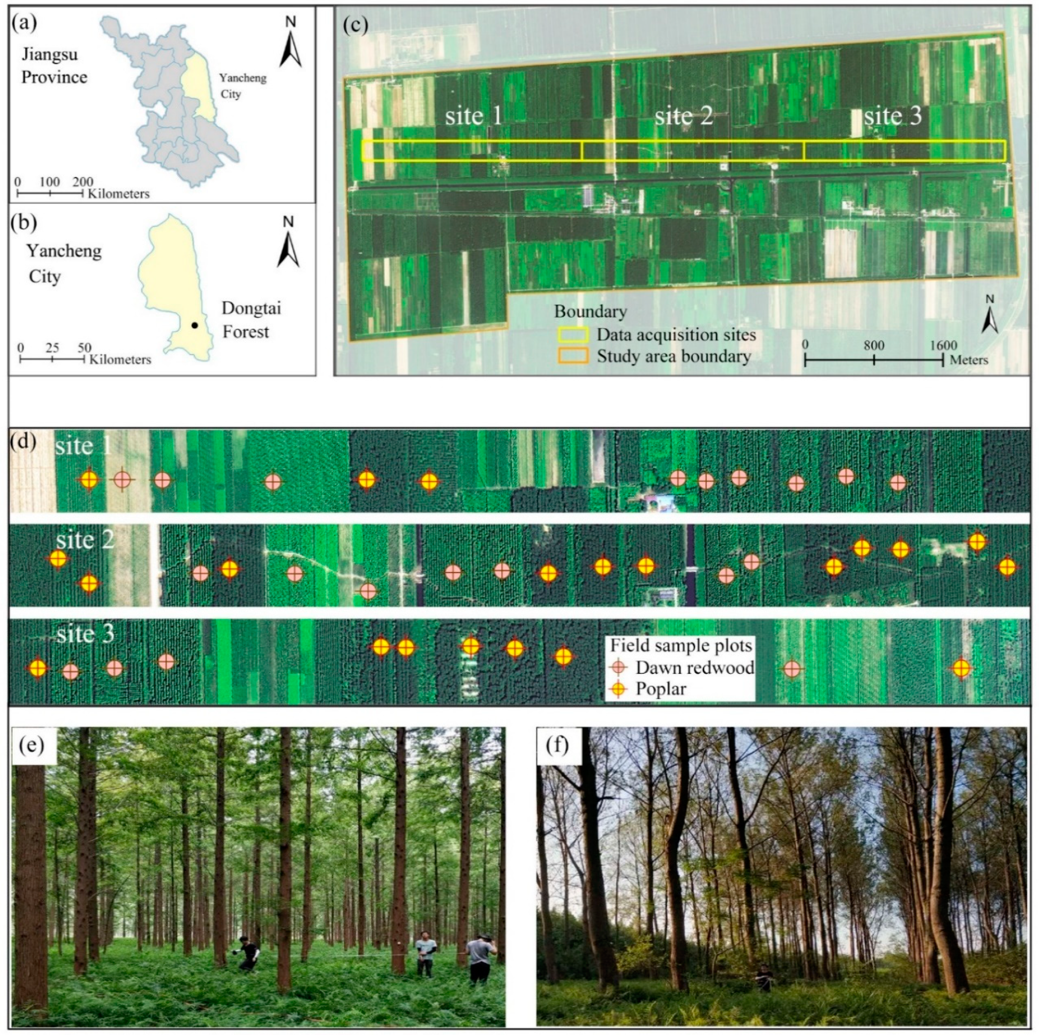
2.1. Study Area

The study area covered approximately 1963 ha and was located in Dongtai Forest, a planted forest in coastal Jiangsu province, east China (120°49′32.2″ E, 32°52′20.6″ N). The annual mean temperature is 14.6 °C, and the annual mean precipitation is 1050 mm [41]. The topography within the study area is flat, and the mean elevation ranges from 11 to 14 m above sea level. The major planted tree species include dawn redwood and poplar. Figure 1 shows the location of the study area and field sample plots for both tree species, as well as the photos of two typical plots.

2.2. Field Data

The field data within the study area were collected from 11–18 September 2016, and were based on the dominant tree species, age classes, and site index of historical survey data; a total of 41 circular plots (radius (r) = 15 m) were set in the data acquisition sites (Figure 1c). All plots (n = 41) were divided into a dawn redwood group (n = 20) and a poplar group (n = 21) according to the tree species composition. The centers of field plots were positioned according to Trimble GeoXH6000 global positioning system (GPS) (Trimble, Sunnyvale, CA, USA) units, which were corrected with high-precision real-time differential signals received from the Jiangsu Continuously Operating Reference Stations (JSCORS), resulting in a sub-meter accuracy [41]. DBH was measured using a diameter tape, and tree-top height was measured using a Vertex IV hypsometer (Haglöf, Långsele, Sweden). Based on the measurement data, a number of forest structural attributes for each plot were calculated, including average DBH (cm), Lorey’s mean height (m) (i.e., mean height weighted by basal area), stem density (n·ha⁻¹), basal area (m²·ha⁻¹), volume (m³·ha⁻¹), and aboveground biomass (mg·ha⁻¹). The plot-level volume was calculated using the provincial species-specific volume equations based on DBH (Appendix A (

Table A1. Equations used in this study for calculating volume.

Tree Species	Equations	Parameters
Dawn redwood	V = A × DB × ((E + F × e(G × D))H)C	A = 0.000058777042, B = 1.9699831, C = 0.89646157, E = 1.000438, F = −0.00024755, G = −0.07897864, H = 7101.252.
Poplar	V = A × DB × ((E + F × e(G × D))H)C	A = 0.000050479055, B = 1.9085054, C = 0.99076507, E = 0.9236004, F = 0.0502109, G = −0.09686479, H = −37.80742.

Note: Tree-level volumes of dawn redwood and poplar were calculated using the equation V = A × D^B × ((E + F × e^{(G × D)})^H)^C, where D is the DBH (cm) and A, B, C, E, F, G, and H are coefficients.

)). The aboveground biomass (AGB) components (including stem, branch, and foliage) were calculated by the species-specific allometric equations based on DBH and height that were developed by Ji et al. [42]. A summary of field-measured forest structural attributes is provided in

Table 1. A summary of field-measured forest structural attributes.

Attributes	All Plots (n = 41)			Dawn Redwood (n = 20)			Poplar (n = 21)
	Range	Mean	SD	Range	Mean	SD	Range	Mean	SD
DBH (cm)	6.3–37.1	23.0	8.3	6.3–30.3	19.4	8.4	11.0–37.1	26.3	6.7
H (m)	4.9–33.4	21.2	8.0	4.9–25.4	16.8	7.5	9.7–33.3	25.3	6.1
D (n·ha−1)	142–850	484.8	190.7	425–850	643.9	129.8	142–482	333.3	85.8
G (m2·ha−1)	6.3–40.1	24.9	8.3	6.3–40.1	25.1	9.6	8.5–35.2	24.8	7.1
V (m3·ha−1)	22.9–352.4	191.0	82.1	22.9–352.4	182.3	100.7	44.3–284.6	199.2	60.8
AGB (Mg·ha−1)	20.1–138.2	80.7	30.9	20.1–138.2	79.0	37.3	27.4–130.8	81.6	24.1

Notes: DBH: mean diameter at breast height; H: Lorey’s mean height; D: stem density; G: basal area; V: volume; AGB: aboveground biomass.

.

2.3. UAV Platforms and Sensors

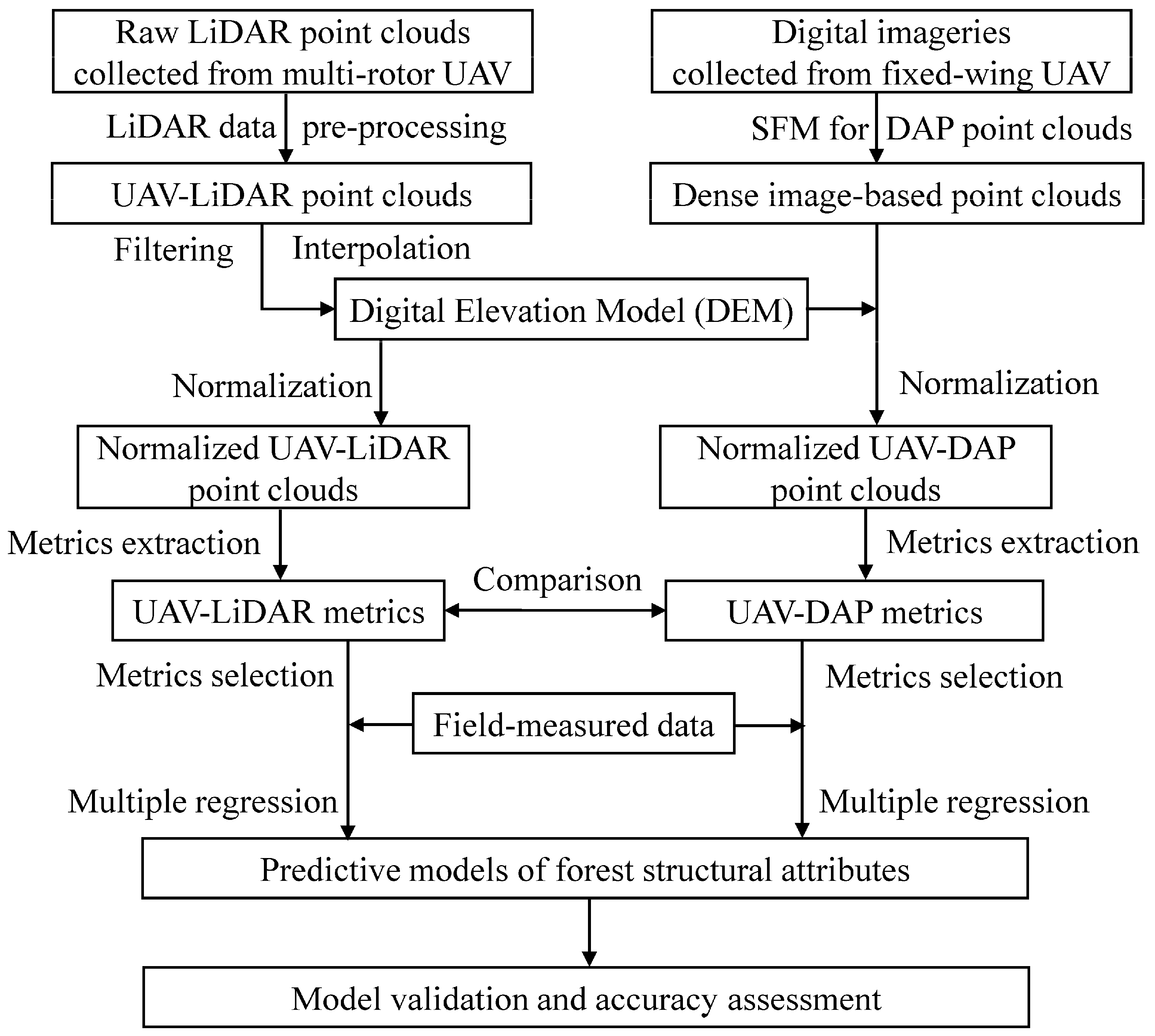
LiDAR data covering the data acquisition sites were acquired using a multi-rotor UAV. High-resolution digital imageries were acquired from a fixed-wing UAV, covering the whole study area (Figure 1c).

The GV1300 (GreenValley International, Berkeley, CA, USA) multi-rotor UAV used in this study was equipped with a Velodyne Puck VLP-16 laser scanner (Velodyne, San Jose, CA, USA) to acquire the LiDAR data. The GV1300 UAV has eight brushless motors, ensuring that the flight has a strong driving force and high stability [43]. The GV1300 UAV was controlled by a ground control station linked with a long-range Wi-Fi system, which transferred information on the real-time trajectory and flying parameters (e.g., flying altitude and speed) supported by a Novatel inertial measurement unit (IMU) (IMU-IGM-S1) and a dual-frequency GPS (Novatel).

The E-DO (E-DO, Shenzhen, China) fixed-wing UAV used in this study was equipped with a Canon EOS 5D Mark II camera (Canon, Japan) to acquire the digital imagery. The flight altitude can reach a maximum of 3500 m with an airspeed of 25 m/s. The UAV was controlled by a custom ground control system using a predefined flight mission. The GPS and IMU of the fixed-wing UAV recorded the longitude and latitude, elevation, roll angle, and pitch angle of each image in real time.

2.4. UAV Data

An overview of the UAV data processing workflow is shown in Figure 2. Firstly, dense image-based point clouds were generated using the SFM algorithm to obtain UAV-DAP point clouds. Secondly, normalized UAV-LiDAR point clouds were generated using a digital elevation model (DEM), which was created based on ground point clouds after filtering; then, the DEM was used to normalize the UAV-DAP point clouds. Thirdly, two suites of metrics were derived from the normalized UAV-LiDAR and UAV-DAP point clouds, and then metric comparisons were conducted under different forest conditions. Finally, the accuracies of predictive models of forest structural attributes, which were generated by UAV-LiDAR and UAV-DAP metrics, were compared. Figure 2 provides an overview of the analysis workflow.

2.4.1. UAV-LiDAR Data and Processing

LiDAR data were obtained from 24–25 August 2016, using a Velodyne VLP-16 laser sensor operating at a flight altitude of 80 m above ground level and a flight speed of 4.8 m/s, which was designed by self-defined trajectories to acquire LiDAR data (Figure 3). The swath width of the LiDAR strip was 42 m. The pulse repetition rate was 18.2 kHz, and the scan frequency was 21.7 Hz, with a maximum scan angle of 30°. The beam divergence was 3 mrad, and the wavelength was 903 nm. The overlap of LiDAR strips was 75%. The average point density of each plot was 50.24 pts·m⁻². Firstly, the LiDAR point clouds were denoised to remove outliers, and the processing was preformed using the Outlier Removal algorithm in LiDAR360 software (GreenValley International, California, CA, USA). The algorithm depends on the average and maximum distance from the point to its neighboring points and the user-defined parameter setting (i.e., neighboring points and multiples of standard deviation) to identify the outlier points. Secondly, the improved progressive Triangulated Irregular Network (TIN) densification (IPTD) filter algorithm was used to classify the ground points [41], and the default parameters were employed in processing (i.e., max building size (m): 20; max terrain angle (°): 88; iteration angle (°): 30; iteration distance (m): 1.6). Then, the DEM (spatial resolution = 0.5 m) was generated using the inverse distance weighting (IDW) interpolation algorithm. Finally, the DEM was subtracted from the elevation value of each point [28,44,45] using the normalization function in LiDAR360 software (GreenValley International, California, CA, USA) for generating normalized point clouds.

2.4.2. UAV Imagery Acquisition and Point Cloud Processing

Digital imagery acquisition was conducted on 7 August 2016, using a Canon EOS 5D Mark II camera with a flight altitude of 500 m above ground level, which covered the whole study area (Figure 1c). The end lap of the flight was 80%, and the side lap was 65%. A fixed camera setting was used during the whole flight to ensure constant radiometry for the imagery [46]. The exposure time was set to 1/1000 s, the focal length was 35 mm, and the aperture value was fixed at f/3.2. The setting of a low Light Sensibility Ordinance (ISO) speed (ISO 250) ensured effective luminosity. The imagery was collected with 0.10 m ground sample distance (GSD). The pixel size was 6.4 μm, and the average point density was 13.10 pts·m⁻². At the same time, 18 ground control points (GCPs) were set within the study area and were located using the Trimble RTK (Real-Time Kinematic). Imagery pre-processing was performed using the SFM algorithm as implemented in Pix4D (Version 4.2.26) (Pix4D S.A., Lausanne, Switzerland) to generate dense image point clouds. The average point density of each plot was 13.10 pts·m⁻². After the DAP processing, DAP point clouds were normalized by the LiDAR-generated DEM to derive heights above ground and obtain normalized DAP point clouds.

2.5. UAV-LiDAR and UAV-DAP Point Cloud Metrics

To compare UAV-LiDAR and UAV-DAP data, two suites of metrics were calculated from normalized UAV-LiDAR and DAP point clouds. i.e., standard and canopy metrics (

Table 2. Description of the metrics derived from unmanned aerial vehicle (UAV) light detection and ranging (LiDAR) and digital aerial photogrammetry (DAP) point clouds that were used for the comparison and modeling forest structural characteristics.

Metrics		Description
Standard metrics
Height-based	Height percentiles (H25, H50, H75, H95)	The percentiles of the canopy height distributions (25th, 50th, 75th, and 95th) above 2 m.
	Mean height (Hmean)	Mean of return heights above 2 m.
	Coefficient of variation of heights (Hcv)	Variation of heights of LiDAR returns above 2 m.
	Maximum height (Hmax)	Maximum of return heights above 2 m.
Density-based	Canopy return density (D3, D5, D7, D9)	The proportion of points above the quantiles (30th, 50th, 70th, and 90th) to total number of points above 2 m.
Canopy cover	Canopy cover above mean height (CC2m)	Percentages of LiDAR return heights above 2 m.
	Canopy cover above mean height (CCmean)	Percentages of LiDAR return heights above average point cloud height.
Canopy metrics
Canopy volume	Open and closed gap zones of canopy volume metric (CVM) (i.e., Open and Closed)	The “Empty” voxels were located above and below the canopy, respectively.
	Euphotic and oligophotic zones of CVM (i.e., Euph and Oligo)	The voxels located within an uppermost percentile (65%) of all filled grid cells of that column, and voxels located below the point in the profile, respectively.
Weibull-fitted	Parameter α and β of Weibull distribution	The scale parameter α and shape parameter β of the Weibull density distribution fitted to the canopy height distribution (CHD).

). These metrics included (i) height-based metrics (H₂₅, H₅₀, H₇₅, H₉₅, H_mean, H_cv, and H_max); (ii) density-based metrics (D₃, D₅, D₇, and D₉); (iii) canopy cover (CC_mean); (iv) canopy volume metrics (Open, Euph, Oligo, and Closed); and (v) Weibull-fitted metrics (Weibull α and Weibull β). The descriptions of UAV-LiDAR and UAV-DAP metrics are shown in Table 2.

2.5.1. Canopy Volume Metric Calculation

The canopy volume model (CVM) approach, which was based on voxels, represented the vertical structural distribution of elements in a canopy space [47,48]. The canopy spaces were divided into four parts of three-dimensional crown volume zones (i.e., Open, Euphotic, Oligophotic, and Closed zones). Firstly, according to whether there was a point cloud in the voxel (5 × 5 × 0.5 m³), all voxels of each canopy space were divided into “Filled” and “Empty” voxels. Secondly, the voxels defined as “Filled” were further classified according to their vertical distribution; the uppermost 65% of the “Filled” voxels were classified as the euphotic (“Euph”) voxels and the lowermost 35% as the oligophotic (“Oligo”) voxels, whereas “Empty” voxels continued to be classified as the higher (“Open”) or lower (“Closed”) voxels of the “Empty” voxels. Finally, canopy volume metrics (i.e., Open, Euph, Oligo, and Closed) were calculated as a set of metrics by running a program conducted in MATLAB R2016b software (The Mathworks, Natick, MA, USA). The descriptions of canopy volume metrics are shown in Table 2.

2.5.2. Weibull Metric Calculation

The canopy height distribution (CHD) profile described the vertical distribution of point clouds, which characterized the condition of the foliage elements and the non-photosynthetic tissues within the canopy [19]. According to previous studies [19,47], the same height interval (0.3 m) was selected so that the results could be compared. All point clouds of the canopy space were sliced into the same interval of stratified layers from the ground to the top of canopy, and the ratio of the number of point clouds to the total point cloud in a certain height interval was calculated, which represented the vertical distribution of the point clouds [49,50]. The Weibull function reflects the distribution of different tree species [51,52], as well as the height distribution of the canopy [53]. Thus, in this study, a Weibull density function was used to fit the CHD, and the Weibull-fitted parameters (parameter α and parameter β) were derived to represent Weibull-fitted metrics. Parameter α was the shape parameter (i.e., the vertical scaling and positioning factor), and β was the scaling parameter (i.e., the capability to control the increase or decrease in the width of the distribution) [19]. A detailed description of the metrics is shown in Table 2.

$$F\left(z\right)={{\displaystyle \int }}_{z1}^{z2}CHD\left(z\right)dz,$$

(1)

$$F\left(z\right)=1-\left(e^{-{\left(\frac{1-\frac{z}{H_{max}}}{\alpha }\right)}^{\beta }}\right),$$

(2)

where $F\left(z\right)$ is the cumulative CHD function, $CHD\left(z\right)$ is the CHD value of $z1$ and $z2$ stratified intervals with a change in the height of CHD, $z$ is the height above the ground, and $H_{max}$ is the maximum height of the canopy.

2.6. Metric Selection and Regression Analysis

In this study, a number of metrics were extracted to assess the accuracies of the predictive models of forest structural attributes. To quantitatively compare the difference between UAV-LiDAR and UAV-DAP metrics, the mean difference (MD), the root-mean-square deviation (RMSD), and Pearson’s correlation coefficient (r) were used in this study (see details in White et al. (2015) [28]). MD represented the average difference between two suites of metrics, RMSD indicated the general level of difference, and r represented the correlation between UAV-LiDAR and UAV-DAP metrics. Previous studies [47,54] provided helpful references for the selection of metrics that proved useful in predictive models. Pearson’s correlation coefficient (r) was used to analyze the relationships between forest structural attributes and all of the metrics (i.e., height-based, density-based, canopy cover, canopy volume, and Weibull-fitted metrics). The metrics with low correlation (r < 0.2) were eliminated, and other metrics were selected for use in the regression analysis.

The multiple regression models were separately fitted to predict the forest structural attributes (i.e., mean DBH, Lorey’s mean height, stem density, basal area, volume, and aboveground biomass) using UAV-LiDAR and UAV-DAP metrics. All dependent variables (forest structural attributes) and independent variables (derived metrics) were transformed using the natural logarithm for linearity and were corrected for bias using a bias correction factor (BCF) [55]. F-tests were applied, and the independent variables with a p < 0.05 significance level were kept in the model. Multicollinearity was assessed by principal component analysis (PCA) based on the correlation matrix to ensure a relatively low correlation between independent variables. Models with a low condition number (k < 30) were selected to reduce multicollinearity [56]. Finally, the best predictive models were selected based on Akaike information criterion (AIC) [57]. The accuracies of the predictive models were evaluated using the coefficient of determination (R²), adjusted R² (Adj-R²), root-mean-square error (RMSE), and relative root-mean-square error (rRMSE), defined as the percentage of the ratio of RMSE and the observed mean values, the root-mean-square error (RMSE) of the adjustment decision coefficient (Adj-R²), and the relative RMSE (rRMSE). After selecting the optimal model, leave-one-out cross-validation was used to evaluate the accuracies of the predictive models [58]. Equations (3)–(6) were used as follows:

$$R^2=1-\frac{{\displaystyle \sum _{i=1}^n{(x_i-{\widehat{x}}_i)}^2}}{{\displaystyle \sum _{i=1}^n{(x_i-{\overline{x}}_i)}^2}}$$

(3)

$$\mathrm{Adj}-R^2=1-\frac{\mathrm{n}-1}{\mathrm{n}-\mathrm{p}-1}(1-R^2)$$

(4)

$$RMSE=\sqrt{\frac{1}{\mathrm{n}}{\displaystyle \sum _{i=1}^{\mathrm{n}}{(x_i-{\widehat{x}}_i)}^2}}$$

(5)

$$rRMSE=\frac{RMSE}{\overline{x}}\times 100\%$$

(6)

where $x_i$ represents the field-measured values for plot $i$; $\overline{x_i}$ represents the average field-measured values for plot $i$; ${\widehat{x}}_i$ represents the estimated values for plot $i$; $\overline{x}$ represents the average field-measured values for all plots; $p$ is the number of variables; $n$ is the number of plots; and $i$ is the sample number.

3. Results

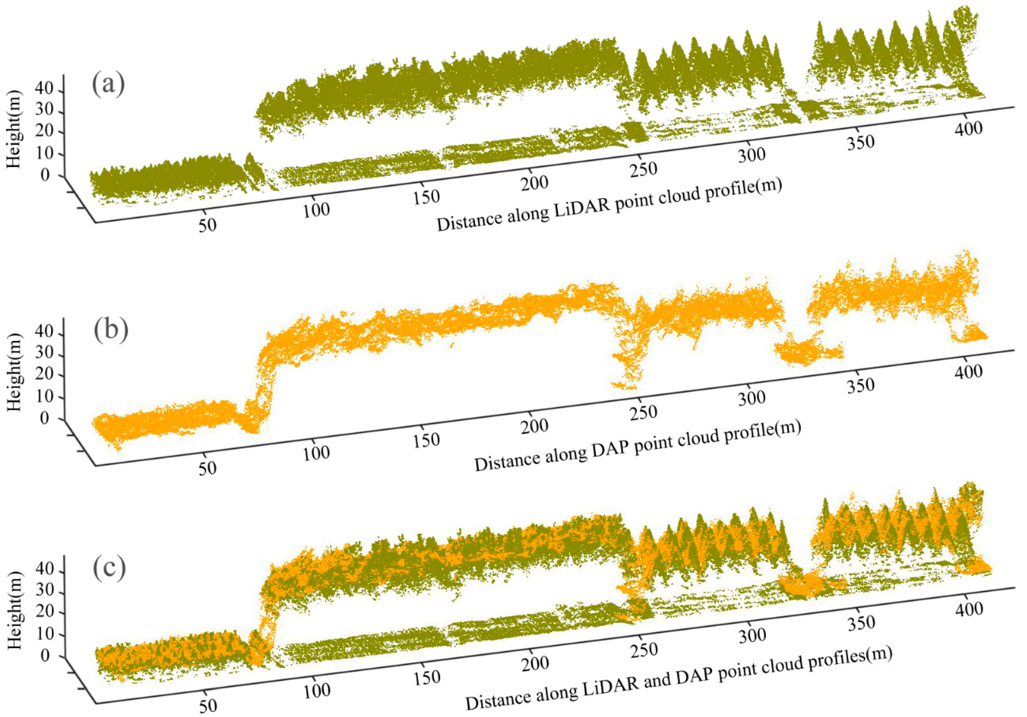
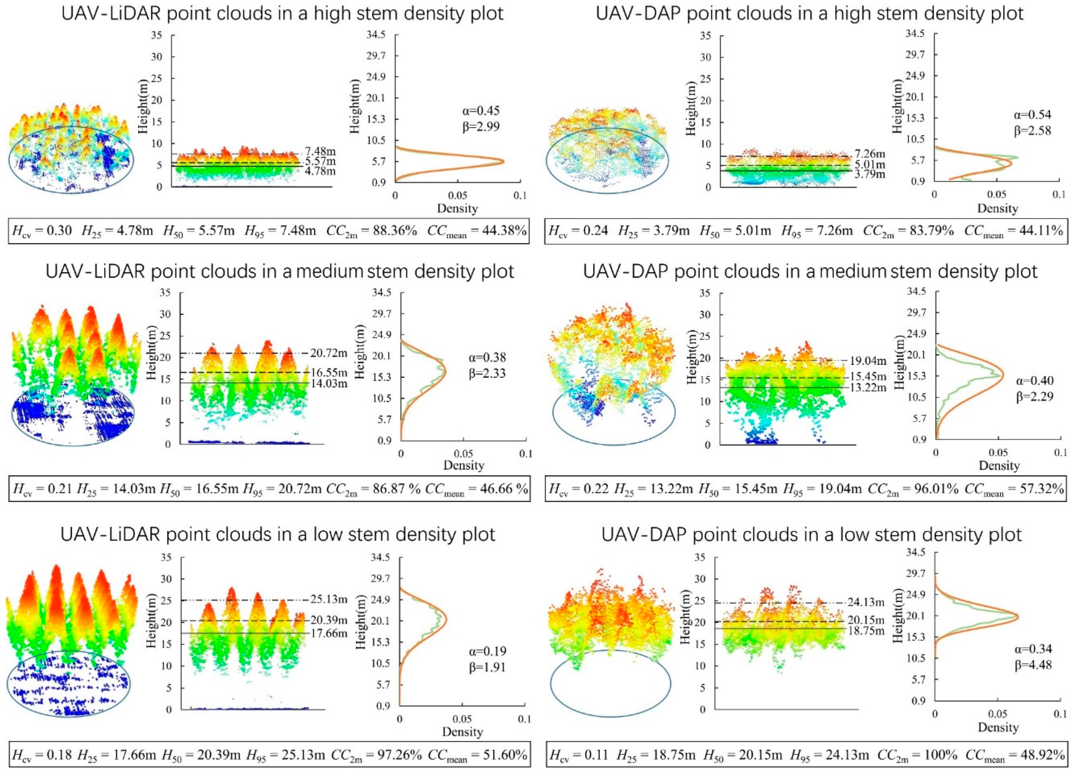
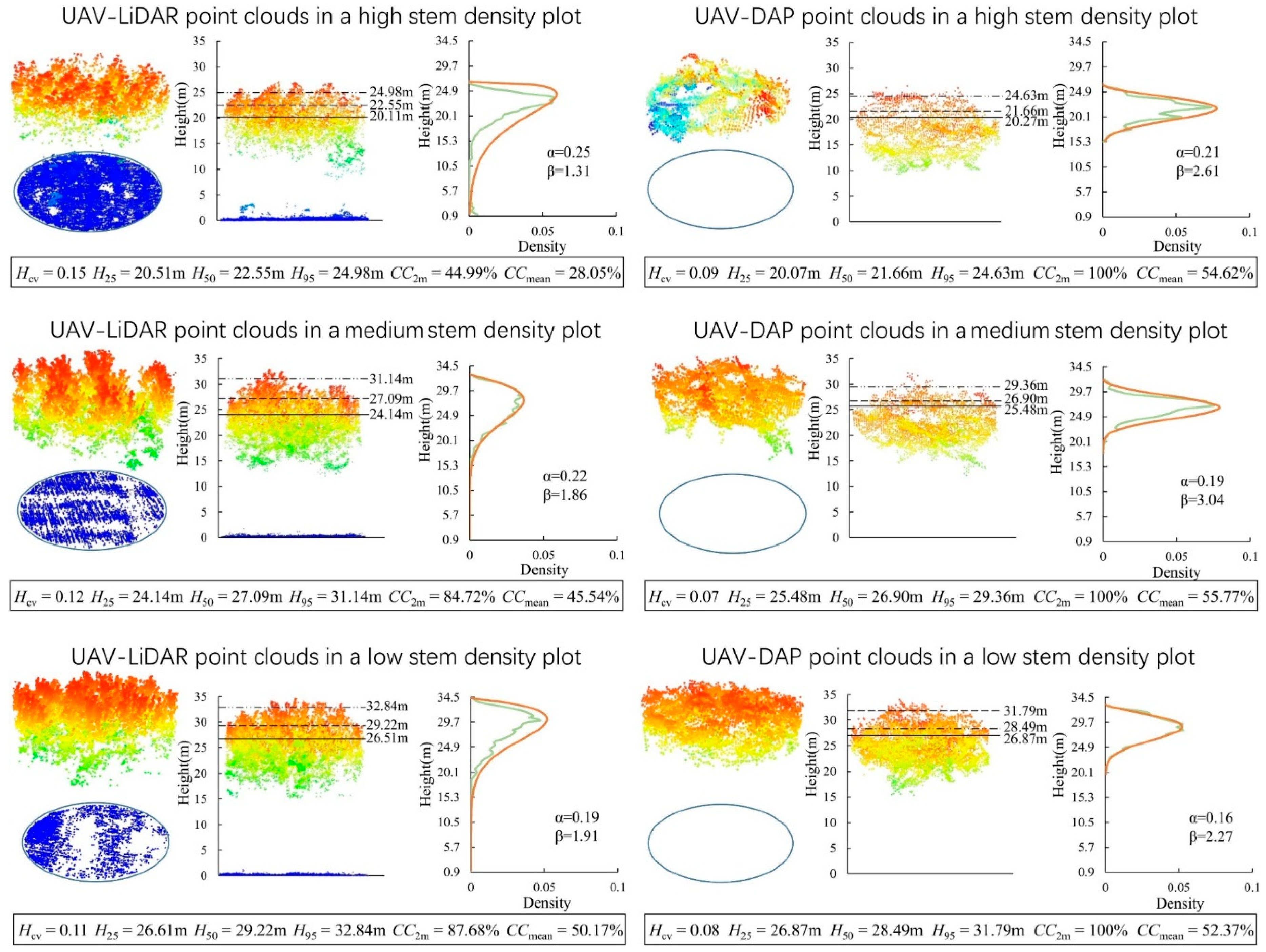
3.1. Visual Comparison of UAV-LiDAR and UAV-DAP Point Clouds and Metrics

The comparison of a UAV-LiDAR and UAV-DAP strip, across forest stands with different tree species, heights, and stem densities, is shown in Figure 3. A total of 1230 images were generated from SFM and resulted in a GSD with 0.1 m. The GCPs made it effective to align the LiDAR and DAP data. A total of 18 GCPs were used in the processing of image matching, resulting in a mean RMSE of 0.012 m.

Three typical sample plots (with different stem densities) for each tree species, i.e., dawn redwood (Figure 4) and poplar (Figure 5), were selected for visual comparison by analyzing the point cloud profiles and height distributions. Overall, UAV-DAP point clouds had similarities with UAV-LiDAR point clouds in the vertical distributions, and the difference in the height percentile metrics between the two data sources for dawn redwood plots showed higher similarity than that for the poplar plots. For dawn redwood plots (Figure 4), the difference value (DV, i.e., the absolute differences between UAV-LiDAR and UAV-DAP metrics) of H₉₅ (the 95th percentile of heights) varied from 0.22 m to 1.68 m, the DV of H₂₅ (the 25th percentile of heights) varied from 0.99 m to 1.09 m, and the plot with the highest density exhibited the smallest difference. For the coefficient of variation of heights (H_cv), the DV of the two data sources ranged from 0.01 to 0.07. For poplar plots (Figure 5), the difference in H₉₅ was higher than that in dawn redwood plots, with the DV ranging from 0.35 m to 1.78 m, but no similar trend was detected for H₂₅ (DV = 0.16–1.34 m). The DV of H_cv ranged from 0.03 to 0.06, and H_cv of UAV-LiDAR was higher than UAV-DAP.

For canopy cover above 2 m (CC_2m) and canopy cover above mean height (CC_mean), generally, CC_2m (ΔDV = 2.74–55.01%) showed a greater difference than CC_mean (ΔDV = 0.27–26.57%). However, there was a greater disparity in CC_2m of poplar plots than that of dawn redwood plots. Additionally, ΔDV = 0.27–10.66% for dawn redwood plots and 2.2–26.57% for poplar plots. The results showed CC_mean with ΔDV = 2.74%–9.17% for dawn redwood plots and 12.32%–55.01% for poplar plots. Canopy height distribution (CHD) profiles are shown in Figure 4 and Figure 5. Weibull curves (orange line) were used to fit CHDs, and the Weibull shapes of UAV-LiDAR were slightly steeper than those of UAV-DAP. It was evident that the Weibull scales of UAV-LiDAR were slightly larger than those of UAV-DAP. The peak of the Weibull curves of UAV-LiDAR was higher than seen for UAV-DAP, especially in poplar plots.

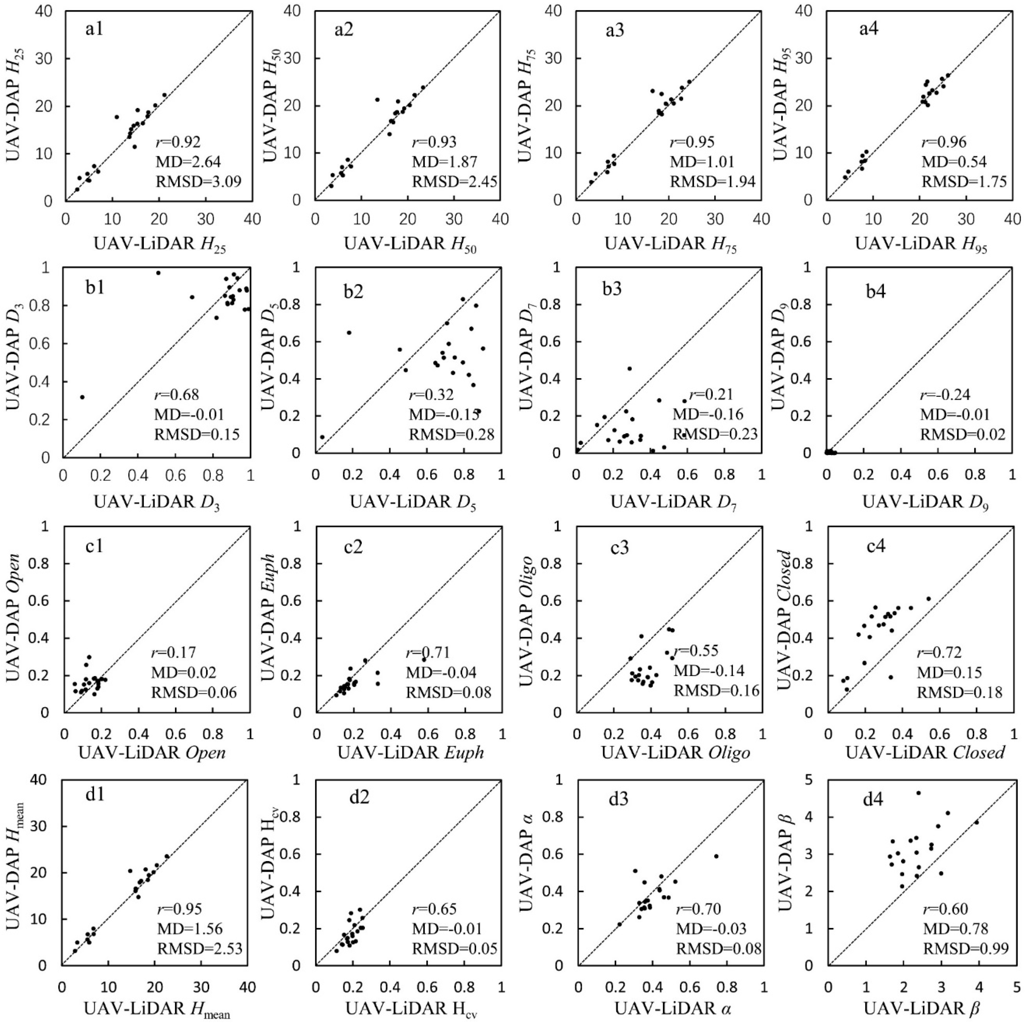
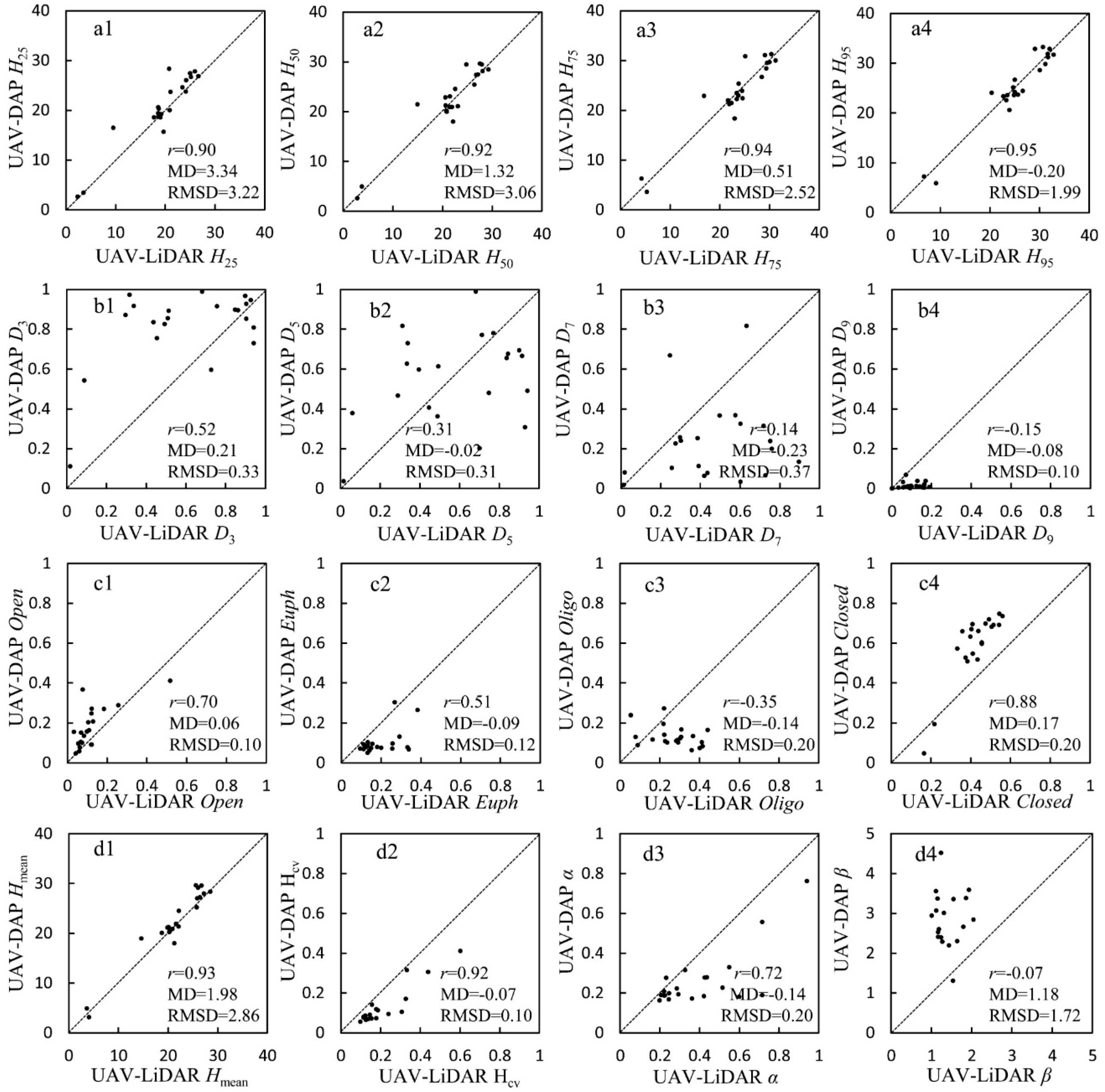
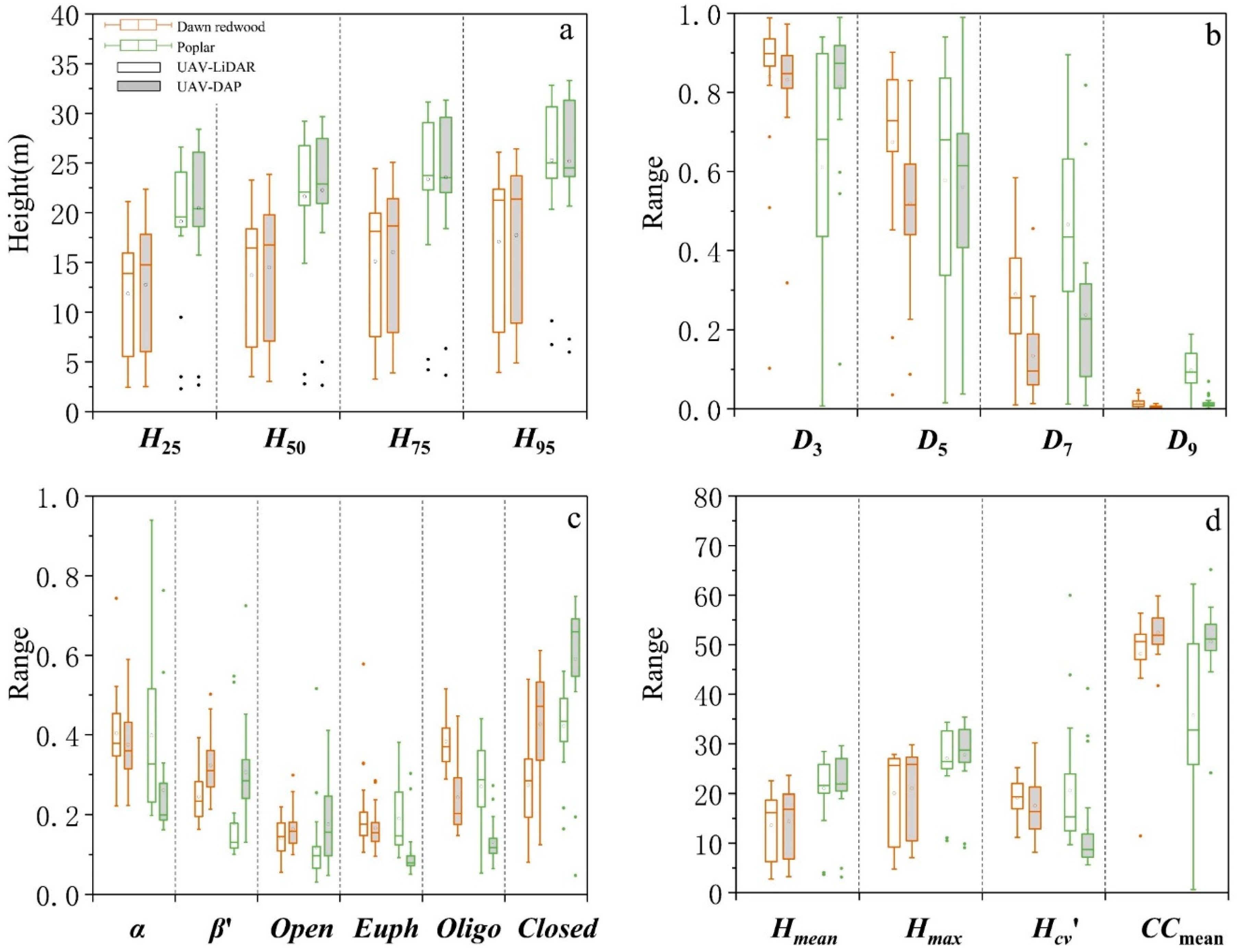
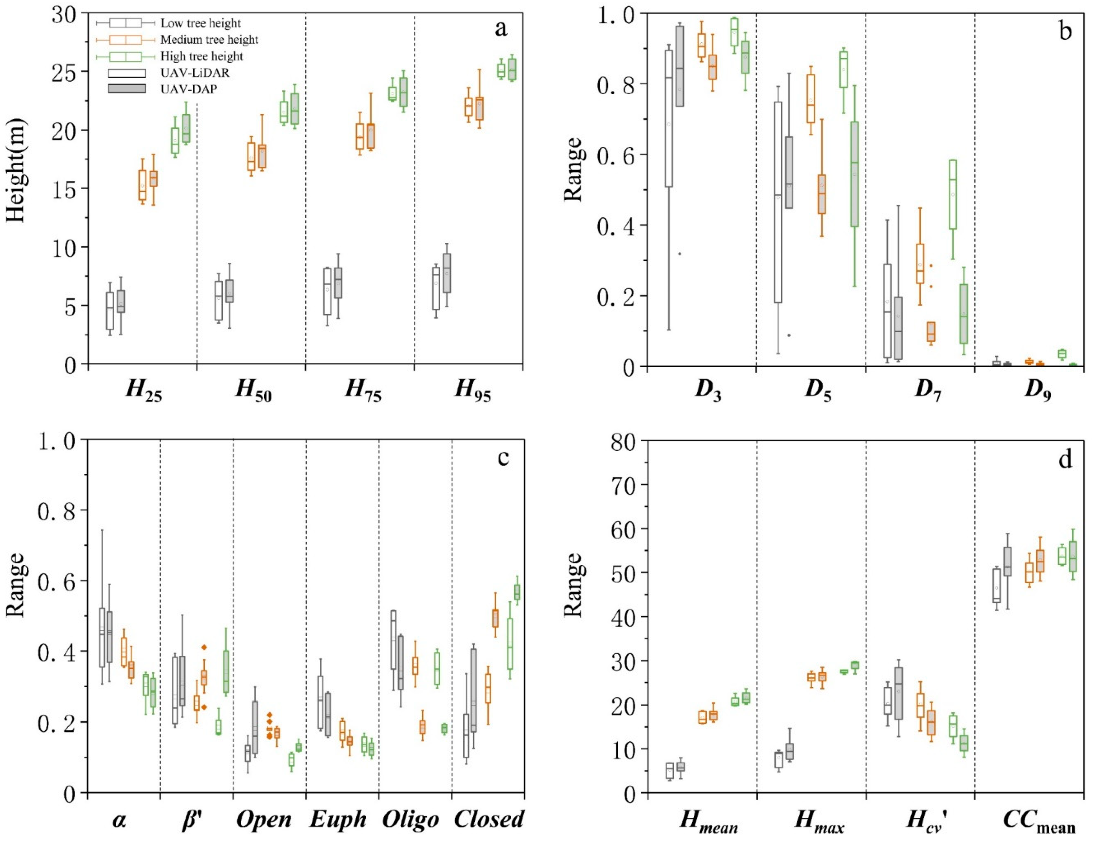
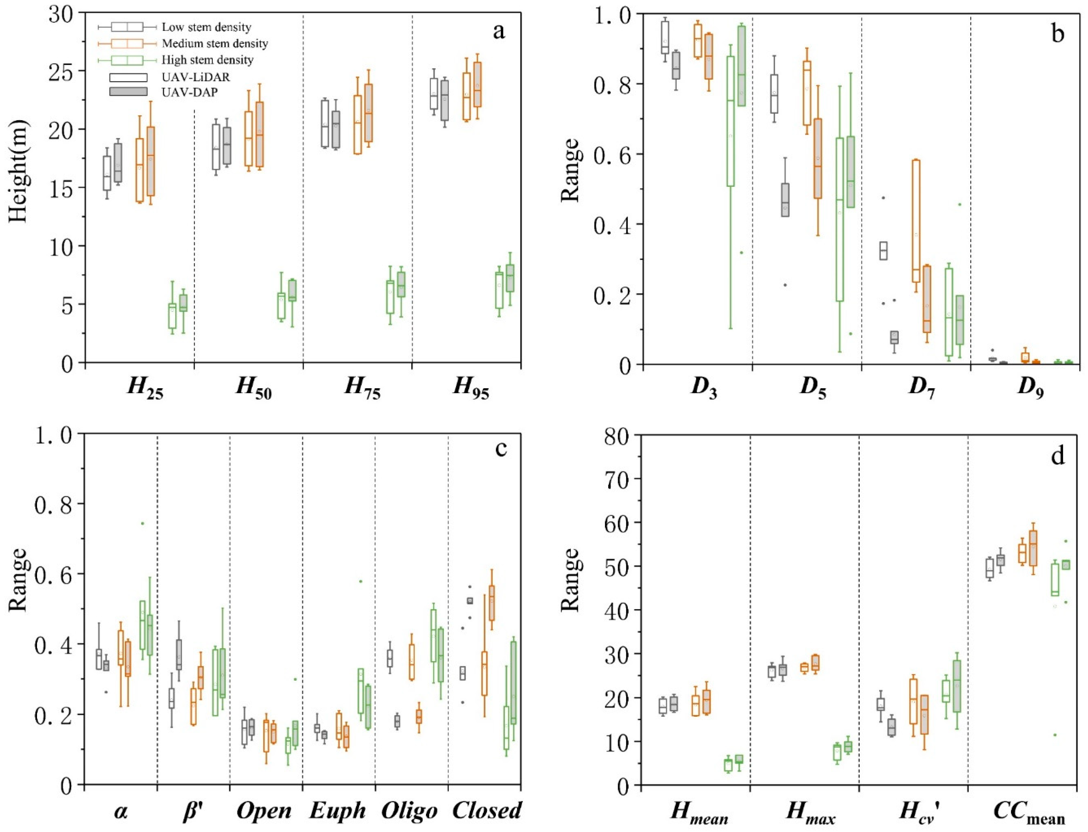
3.2. Statistical Comparison of UAV-LiDAR and DAP Metrics

Figure 6 and Figure 7 show the results of scatterplots of UAV-LiDAR and UAV-DAP metrics in dawn redwood and poplar plots, respectively. In general, the metrics of the upper percentiles (r = 0.95–0.96, 0.94–0.95) showed a higher correlation than those of lower percentiles (r = 0.92–0.93, 0.90–0.92), whereas the metrics of the upper canopy return density (r = 0.21–0.24, 0.14–0.15) showed a lower correlation than those of the lower canopy return density (r = 0.32–0.68, 0.31–0.52). The metric of the closed zone showed the highest correlation (r = 0.72–0.88) within the canopy volume profile model-derived metrics. The Weibull α parameter indicated a relatively high correlation (r = 0.70–0.72), and showed a trend that the height-based metrics had a stronger correlation than the other metrics. The correlations for dawn redwood plots were higher than those for poplar plots in both height-based and density-based metrics. For height percentiles, MD varied from 2.64 to 0.54, whereas RMSD ranged from 3.09 to 1.75, which showed a decreasing trend.

Figure 8 shows the comparison of two suites of metrics using boxplots; metrics were selected to compare dawn redwood (red plot) and poplar plots (green plot). The white-filled plot (left) represents UAV-LiDAR metrics, whereas the gray-filled plot (right) represents UAV-DAP metrics. The transverse line of each box represents the median value, and the circle within the plot represents the average value. In total, all metrics were classified into four groups. In general, for height percentiles, poplar plots showed slightly higher heights compared with dawn redwood. For both tree species, the similarities between the two suites of metrics increased with increasing percent height. The difference in the median and average value for poplar was larger than that for dawn redwood in general. The median value of DAP was higher than that of LiDAR for all height percentiles in dawn redwood plots. Plots of DAP metrics showed slightly higher heights compared with LiDAR metrics from H₂₅ to H₅₀, and then become lower than LiDAR metrics. For density-based metrics, the variation of poplar plots was larger than that of dawn redwood plots. For the Weibull parameters, the difference in α was smaller than that in β. H_mean and H_max were similar between the two suites of metrics. Other metrics exhibited no significant similarity.

In this study, to further analyze the influence of forest conditions on DAP, we selected dawn redwood plots with different heights and stem densities. Figure 9 shows a comparison between two suites of metrics in dawn redwood plots, which were grouped by field-measured Lorey’s mean height (i.e., low, medium, and high tree heights). In general, plots with high height presented greater similarities than did low and medium height plots. The height percentiles seemed to be similar for all plots, but the median line indicated a small difference in low and high heights and a lower variation in medium- and high-height plots. For density-based metrics, plots with low height showed greater variation than other height plots. For canopy volume metrics, plots with low height and high height performed better. For other metrics, in Figure 9d, there was no obvious difference for all plots, except for CC_2m. Therefore, considering height-grouped plots, plots with greater height were relatively stable for both UAV-LiDAR and UAV-DAP.

Figure 10 shows another grouping method for assessing the two suites of metrics. All dawn redwood plots were grouped into different stem densities (i.e., low, medium, and high stem densities), according to the field-summarized stem density data. In general, Figure 10 indicates that plots with lower stem densities had more similarity than other stem densities plots. For height percentiles, the median line was closer for low-stem-density plots than for medium-stem-density plots, whereas the variation of boxplots was the largest for high-stem-density plots. For density-based metrics, according to the median line and the variation of boxplots, high-stem-density plots had more similarity. For canopy volume metrics, plots with low stem density had more similarity in α and Open metrics than did other grouped plots, whereas plots with high stem density had more similarity in β’ than did other grouped plots. For other metrics, low-stem-density plots were more similar than other plots in H_mean and H_max. In general, low-stem-density plots had relatively greater similarity for UAV-LiDAR and UAV-DAP.

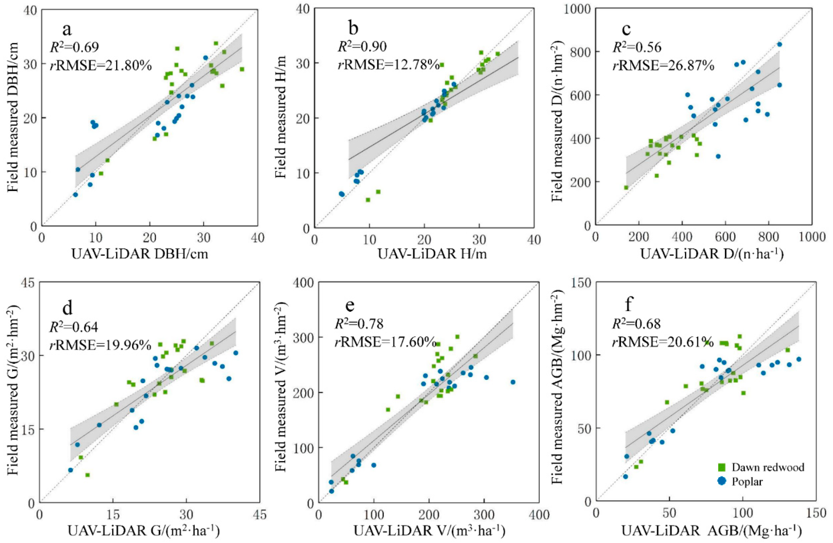
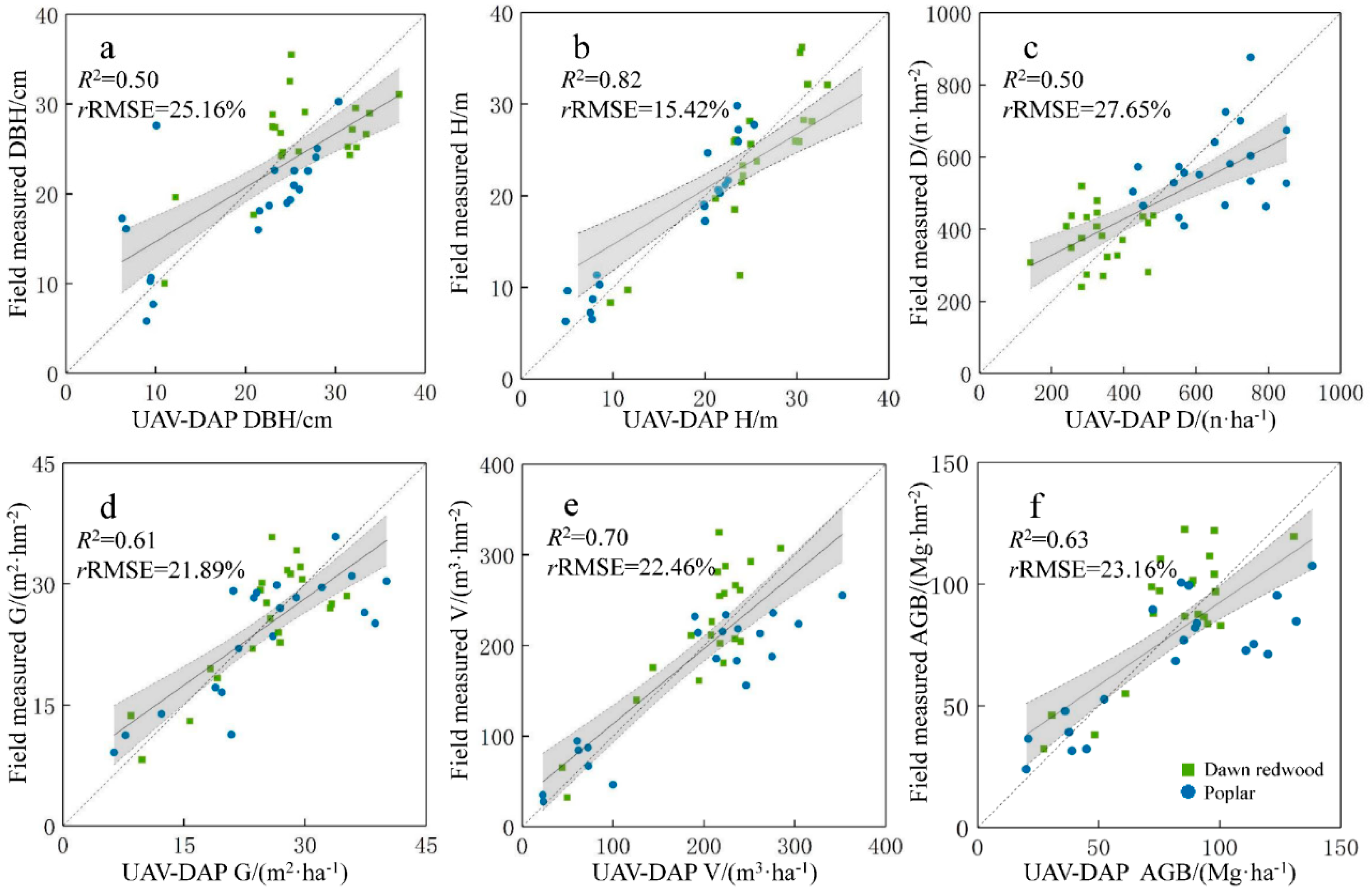
3.3. Forest Structural Attribute Modeling and Accuracy Assessment

In this study, a number of forest structural attributes were evaluated using the multi-regression models with UAV-LiDAR and UAV-DAP metrics alone, as well as the integration of LiDAR and DAP metrics (see

Table 3. A summary of predictive models and accuracy assessment results. Adj-R²: adjusted R²; RMSE: root-man-square error; rRMSE: relative RMSE.

Attributes	Predictive Models	R2	Adj-R2	RMSE	rRMSE (%)
DBHlidar	exp(−1.02 × lnD3 + 1.12 × lnD5 + 0.40 × lnClosed + 3.75) × 1.029	0.72	0.69	4.57	19.92
Hlidar	exp(−0.55 × lnH75 + 1.45 × lnH95 + 0.09 × lnClosed + 0.33) ×1.001	0.92	0.91	1.91	9.03
Dlidar	exp(−0.33 × lnH95 + 0.41 × lnD5 − 0.14 × lnD9 + 6.86) ×1.027	0.61	0.58	117.76	24.29
Glidar	exp(0.41 × lnH95 + 0.28 × lnD7 − 0.11 × lnD9 + 1.93) × 1.017	0.69	0.66	4.58	18.36
Vlidar	exp(0.98 × lnH95 + 0.19 × lnD5 + 0.17 × lnOpen + 2.72) × 1.016	0.81	0.79	26.81	14.04
AGBlidar	exp(0.71 × lnH95 + 0.17 × lnD5 − 0.05 × lnD9 + 2.14) × 1.016	0.73	0.71	15.87	19.75
DBHDAP	exp(−0.48 × lnD5 + 0.21 × lnD7 + 0.73 × lnClosed + 3.77) × 1.047	0.60	0.57	5.17	22.52
HDAP	exp(0.17 × lnH25 + 0.89 × lnH95 − 0.35 × lnD3 − 0.21) × 1.005	0.85	0.83	2.60	12.20
DDAP	exp(0.68 × lnD3 − 0.16 × lnD7 + 0.45 × lnOligo + 6.73) × 1.042	0.56	0.52	125.28	25.84
GDAP	exp(0.83 × lnHmean + 0.28 × lnOligo + 0.33 × lnα + 1.68) × 1.021	0.66	0.63	4.79	19.22
VDAP	exp(1.53 × lnH95 + 0.45 × lnD3 − 0.60 × lnClosed + 0.13) × 1.028	0.73	0.70	34.84	18.24
AGBDAP	exp(1.06 × lnHmean − 0.27 × lnClosed + 0.26 × lnα + 1.46) × 1.020	0.67	0.65	17.42	21.68
DBHL-D	exp(0.80 × lnH95L + 0.11 × lnClosedL + 0.07 × lnβD + 0.75) × 1.021	0.75	0.73	4.26	16.64
HL-D	exp(0.94 × lnH95L − 0.07 × lnD3L − 0.05 × lnOpenD + 0.04) × 1.001	0.95	0.95	1.60	7.20
D L-D	exp(0.44 × lnD3L − 0.10 × lnD9L − 0.31 × lnH75D + 6.84) × 1.022	0.70	0.68	108.58	22.40
GL-D	exp(0.35 × lnH95L + 0.21 × lnD7L + 0.24 × lnβD + 2.15) × 1.015	0.73	0.72	4.51	18.09
V L-D	exp(0.98 × lnH95L + 0.19 × lnD5L + 0.17 × lnOpenD + 2.72) × 1.012	0.86	0.85	22.87	11.21
AGBL-D	exp(0.66 × lnH95L + 0.15 × lnD5L + 0.14 × lnβD + 2.31) × 1.015	0.77	0.76	15.19	18.51

Notes. DBH_lidar: mean diameter at breast height for UAV-LiDAR model; H_lidar: Lorey’s mean height for UAV-LiDAR model; D_lidar: stem density for UAV-LiDAR model; G_lidar: basal area for UAV-LiDAR model; AGB_lidar: aboveground biomass for UAV-LiDAR model; V_lidar: volume for UAV-LiDAR model; DBH_DAP: mean diameter at breast height for UAV-DAP model; H_DAP: Lorey’s mean height for UAV-DAP model; D_DAP: stem density for UAV-DAP model; G_DAP: basal area for UAV-DAP model; AGB_DAP: aboveground biomass for UAV-DAP model; V_DAP: volume for UAV-DAP model; DBH_L-D: mean diameter at breast height for LiDAR-DAP model; H_L-D: Lorey’s mean height for LiDAR-DAP model; D_L-D: stem density for LiDAR-DAP models; G_L-D: basal area for LiDAR-DAP models; AGB_L-D: aboveground biomass for LiDAR-DAP models; V_L-D: volume for LiDAR-DAP models; L in the lower right corner of the variable represents the metrics of LiDAR; D represents the metrics of DAP. L-D represents the metrics of both LiDAR and DAP.

). In general, the integration of LiDAR and DAP metrics performed the best for predicting the forest structural attributes (Adj-R² = 0.73–0.95, rRMSE = 7.20–22.40%). The accuracies of UAV-LiDAR models were higher than those of UAV-DAP models; basal area exhibited the smallest difference (ΔAdj-R² = 0.03, ΔrRMSE = 0.86%), and volume had the greatest difference (ΔAdj-R² = 0.09, ΔrRMSE = 3.55%). The UAV-LiDAR model outcomes showed that the estimation of Lorey’s mean height (Adj-R² = 0.91, rRMSE = 9.03%) and volume (Adj-R² = 0.79, rRMSE = 14.04%) had the highest accuracies, followed by aboveground biomass (Adj-R² = 0.71, rRMSE = 19.75%), DBH (Adj-R² = 0.69, rRMSE = 19.92%), and basal area (Adj-R² = 0.66, rRMSE = 18.36%), whereas stem density (Adj-R² = 0.58, rRMSE = 24.29%) had a relatively low accuracy. The UAV-DAP model outcomes showed that the estimations of Lorey’s mean height (Adj-R² = 0.83, rRMSE = 12.20%) and volume (Adj-R² = 0.70, rRMSE = 18.24%) had the highest accuracies, followed by aboveground biomass (Adj-R² = 0.65, rRMSE = 21.68%), basal area (Adj-R² = 0.63, rRMSE = 19.22%), and DBH (Adj-R² = 0.57, rRMSE = 22.52%), whereas stem density (Adj-R² = 0.52, rRMSE = 25.84%) had a relatively low accuracy.

For the selected metrics of the UAV-LiDAR and UAV-DAP predictive models, H₉₅ (selected seven times in total) and Closed (selected five times in total) were most frequently selected, indicating that these metrics are sensitive and representative of the forest structural attributes. For all predictive models, canopy volume metrics (including Open, Oligo, and Closed) contributed to models that were selected by six out of the 12 total models. The model-predicted and the field-measured results of forest structural attributes predicted by UAV-LiDAR and UAV-DAP metrics are shown in Figure 11; Figure 12, as are the cross-validation results. Overall, the UAV-LiDAR models (R² = 0.56–0.90, rRMSE = 12.78–26.87%) performed better than the UAV-DAP models (R² = 0.50–0.82, rRMSE = 15.42–27.65%).

4. Discussion

4.1. Comparison of UAV-LiDAR and UAV-DAP Point Clouds and Metrics

In this study, we demonstrated the capabilities of UAV-acquired LiDAR and DAP data for estimating forest structural attributes in a coastal planted forest of East China. Although both LiDAR and DAP data can provide three-dimensional information on forest structure, there are differences in detecting the vertical distribution of the canopy [6], resulting in a difference of the variations of LiDAR and DAP metrics. Previous studies [16,21,26,28,59,60,61,62] often acquired the LiDAR and DAP data using airborne platforms or used UAV-DAP data (normalized by the airborne LiDAR-generated DEM) to update forest inventory information [63]. Only a few studies used UAV platforms to acquire both LiDAR and DAP data at the same time [40,43], and the assessments of both types of metrics are limited. In this study, we found UAV-DAP point clouds had similarities with UAV-LiDAR point clouds in the vertical height distribution. The point clouds of the two sensors showed similarity in dawn redwood plots, but not in poplar plots. We visually compared the difference between UAV-LiDAR and UAV-DAP data in six plots with different forest types (coniferous and broadleaved) and different stem densities using point cloud profiles (Figure 4 and Figure 5). Three sample plots (with different stem densities) of each tree species, including dawn redwood (coniferous) and poplar (broadleaved), were selected for a visual comparison. Most UAV-DAP point clouds were limited to the upper canopy, as shown in Figure 4 and Figure 5, because the method lacked the ability to penetrate below the canopy as can UAV-LiDAR, except for the UAV-DAP point clouds of the dawn redwood plot in medium stem density (Figure 4). This effect is likely due to the large gaps (regarding the crown width of an individual tree according to LiDAR point clouds), which may have been caused by harvesting of the individual trees due to their illness. Then, the information for the large gaps was captured by high-resolution images and the image matching algorithm.

Compared with UAV-DAP point clouds of the poplar plots, UAV-DAP point clouds of the dawn redwood plots were more similar to UAV-LiDAR point clouds. This similarity may exist because the dawn redwood has a more regular tree crown shape than the poplar, which facilitated identification by the algorithm. For plots with different stem densities (Figure 4 and Figure 5), visually, UAV-DAP point cloud profiles had similar canopy shapes to those of UAV-DAP, and dawn redwood plots were less different than were poplar plots. Canopy height distribution (CHD) profiles were fitted by Weibull curves. Parameter α represented the shape parameter (i.e., the vertical scaling and positioning factor), and β represented the scaling parameter (the capability to control the increase or decrease in the width of the distribution). We found that the Weibull shapes of UAV-LiDAR were slightly steeper than those UAV-DAP, while the Weibull scales of UAV-LiDAR were slightly larger than those of UAV-DAP. This difference may be caused by the concentrated distribution of LiDAR point clouds and the relatively wide distribution of DAP point clouds. In this study, we compared the correlation of UAV-LiDAR and UAV-DAP metrics using traditional metrics and canopy metrics (Figure 6 and Figure 7) for different tree species. The comparison results between the UAV-LiDAR and DAP metrics showed that the metrics of upper percentiles (r = 0.95–0.96, 0.94–0.95) exhibited a higher correlation than the lower percentiles (r = 0.92–0.93, 0.90–0.92), whereas the metrics of upper canopy return density (r = 0.21–0.24, 0.14–0.15) exhibited a lower correlation than those of lower canopy return density (r = 0.32–0.68, 0.31–0.52). The Weibull α parameter indicated a relatively higher correlation (r = 0.70–0.72) than the Weibull β parameter (r = 0.07–0.60) for both dawn redwood and poplar plots. Because DAP was limited to characterizing the outer canopy, most point clouds were focused on the surface of the canopy, whereas the capability to acquire understory forest information was limited. The upper metrics of DAP reflected the canopy surface, which was able to be well characterized by LiDAR. In contrast, the lower metrics did not adequately represent the structural characteristics of the understory. In general, dawn redwood plots (Figure 6) had greater correlation than poplar plots (Figure 7). The difference of H₂₅ and H₉₅ in the poplar plots between UAV-LiDAR and UAV-DAP metrics was greater than that in the dawn redwood plots, because poplar (broadleaf) has structural instability and is easily disturbed by strong wind or heavy snow. The H_cv of UAV-LiDAR was larger than that of UAV-DAP, indicating the ability of LiDAR to penetrate through the forest canopy and obtain the below-canopy information, and highlighting the limitation of DAP in characterizing the outer canopy information; the same trend was reported in previous studies [6].

The boxplot of UAV-LiDAR and UAV-DAP metrics (Figure 8) showed that the difference in height-based metrics was the smallest and that the ranges of plots varied closely. Compared with the median line of plots, as the height percentiles increased, UAV-LiDAR and UAV-DAP data were closer to each other, indicating the similarity of the two suites of metrics, which is the same trend as that exhibited by the height percentile metrics in Figure 6 and Figure 7. There were similar increases for UAV-LiDAR and UAV-DAP data as the height percentiles increased, as Vastaranta et al. (2013) found [59]. In this study, in order to further analyze the influence on forest conditions for DAP, we selected dawn redwood plots with different heights and stem densities to assess the variations of the plots (Figure 9 and Figure 10). In general, the higher similarity between the UAV-LiDAR and DAP metrics appeared in the dawn redwood plots with higher height and lower stem density. One of the reasons may be that, in more open forest, the DAP point clouds resemble more the LiDAR ones since it is possible to obtain photogrammetric points in canopy gaps, thus providing more height variation in DAP point clouds. In this study, by comparing the different stem densities of dawn redwood plots, it was found that lower-stem-density plots had more similarity than other plots. The reason for this similarity may be that, in a mature forest, low-stem-density plots are related to taller trees and, thus, can provide more distinguishing characteristics. To meet the needs of silvicultural treatments in planted forests, young trees were usually planted with high density. With the increase in tree height and canopy width, thinning was applied to ensure the robust growth of the stand, which reduced the stem density. Therefore, in this study, the medium- and high-density plots were mostly young and middle-aged forest stands, while the low-density plots were mature forests. Mature forests have a relatively stable stand structure and canopy information, which increases the probability that the image matching algorithm will capture feature elements, thus improving the similarity between UAV-LiDAR and UAV-DAP.

4.2. Forest Structural Attribute Modeling and Accuracy Assessment

As reported by Wallace et al. (2016) [43] with respect to the estimation of forest attributes, more forest structural attributes should be examined with the rapid development of sensor technology and the application of new analysis methods to data collected from UAVs [34,64]. In this study, we assessed more forest structural attributes (i.e., DBH, Lorey’s mean height, stem density, basal area, volume, and aboveground biomass) using UAV-LiDAR and UAV-DAP metrics combined with field-measured data. The accuracies of UAV-LiDAR (Adj-R² = 0.58–0.91, rRMSE = 9.03–24.29%) predictive models for forest structural attributes were relatively higher than those of UAV-DAP (Adj-R² = 0.52–0.83, rRMSE = 12.20–25.84%) models. We found the greatest difference between UAV-LiDAR and UAV-DAP predictive models for volume (ΔAdj-R² = 0.09, ΔrRMSE = 4.20%) and the lowest difference for basal area (ΔAdj-R² = 0.03, ΔrRMSE = 0.86%). The UAV-LiDAR model outcomes showed that the estimation of Lorey’s mean height (Adj-R² = 0.91, rRMSE = 9.03%) and volume (Adj-R² = 0.79, rRMSE = 14.04%) had the greatest accuracies, followed by aboveground biomass (Adj-R² = 0.71, rRMSE = 19.75%), DBH (Adj-R² = 0.69, rRMSE = 19.92%), and basal area (Adj-R² = 0.66, rRMSE = 18.36%), whereas stem density (Adj-R² = 0.58, rRMSE = 24.29%) had a relatively lower accuracy. The UAV-DAP model outcomes showed that the estimation of Lorey’s mean height (Adj-R² = 0.83, rRMSE = 12.20%) and volume (Adj-R² = 0.70, rRMSE = 18.24%) had the greatest accuracies, followed by aboveground biomass (Adj-R² = 0.65, rRMSE = 21.68%), basal area (Adj-R² = 0.63, rRMSE = 19.22%), and DBH (Adj-R² = 0.57, rRMSE = 22.52%), whereas stem density (Adj-R² = 0.52, rRMSE = 25.84%) had a relatively lower accuracy. Hall et al. (2005) [65] used airborne LiDAR data to estimate stand structural attributes in the Colorado Front Range, USA. The results showed that Lorey’s mean height (R² = 0.87, standard error = 0.69) had the highest accuracies, followed by aboveground biomass (R² = 0.74, standard error = 0.20) and stem density (R² = 0.67, standard error = 0.36). Bottalico et al. (2017) [66] modeled several forest structural attributes using airborne LiDAR-derived metrics in Italy. The model results indicated that Lorey’s mean height had the highest accuracy (R² = 0.83, rRMSE = 10.5%) among all the extracted attributes. White et al. (2015) [28] selected complex coastal natural forest as the study area. LiDAR and DAP metrics were separately derived from airborne LiDAR and DAP point clouds; then, the point cloud metrics and plot-level models for Lorey’s height, basal area, and gross volume were compared. The results showed that the most significant difference in the predicting models of the two data sources was for Lorey’s mean height (ΔrRMSE = 5.04%), followed by gross volume (ΔrRMSE = 3.63%), and the lowest difference was for basal area (ΔrRMSE = 2.33%).

There are two reasons explaining the higher accuracies of UAV-LiDAR models than those of UAV-DAP models. One is that DAP point clouds have limited capability to penetrate through the forest canopy and acquire the vertical distribution information for the whole canopy, which leads to a lower ability to estimate forest structural attributes [28,59,67]. The other is that DAP data can be affected by image quality, thereby further impacting the image matching algorithm [27,59]. The lower accuracies of models for UAV-DAP can be partly attributed to shadows and occlusions from surrounding trees or the occasional shaking of leaves, especially in broadleaf stands, which may impact the algorithm. Zhang et al. (2017) [47] used airborne LiDAR data and extracted canopy metrics to estimate forest structural parameters in a north subtropical secondary forest. The results indicated that the estimation accuracies of Lorey’s mean height (Adj-R² = 0.61–0.88) and aboveground biomass (Adj-R² = 0.54–0.81) models were the highest, followed by volume (Adj-R² = 0.42–0.78), DBH (Adj-R² = 0.48–0.74), and basal area (Adj-R² = 0.41–0.69), whereas stem density (Adj-R² = 0.39–0.64) models were relatively lower. The models showed lower accuracies than in the study for Lorey’s mean height (Adj-R² = 0.83–0.91), aboveground biomass (Adj-R² = 0.65–0.71), volume (Adj-R² = 0.70–0.79), DBH (Adj-R² = 0.57–0.69), basal area (Adj-R² = 0.63–0.66), and stem density (Adj-R² = 0.52–0.58). It was likely that the planted forest in this study had a simpler and more homogeneous forest structure than the secondary forest, resulting in higher estimation accuracies.

4.3. Limitations of DAP Point Clouds and Future Works

The results of this study indicated that DAP with a lower point density than LiDAR may not strongly affect the estimation accuracies of plot-level forest structural attributes, although DAP point clouds exhibited higher density than LiDAR in some other studies [26,28,60]. Recently, Lin et al. (2011) [68] found that, compared to airborne LiDAR, UAV-based LiDAR improved point density to support forest measurement with higher precision. Dandois and Ellis (2015) [69] used the SFM algorithm to produce DAP point clouds of temperate deciduous forests at different UAV altitudes and image overlaps. They found that accurate estimates of canopy height were obtained under higher overlap (>80%) conditions, while no significant differences were found in height error at different altitudes (20–80 m) with their own GSD (0.8–3.4 cm). The authors considered the overlap to be crucial for DAP. According to their research, based on UAV-DAP data, the accuracy of estimations of forest structural attributes may be enhanced with higher overlap. However, due to the large difference between altitudes, this possibility deserves further studies to assess the variations of DAP and LiDAR metrics across different altitudes.

One limitation of DAP point clouds generated from the SFM algorithm is that the accuracy and effectiveness of SFM may be affected by the collection of imageries under different forest conditions. As this study indicated, the imageries were difficult to match, and resulted in higher error rates when using forests with the condition of lower mean tree height and higher stem density. Additionally, to some extent, shadows and occasional vibrations of the UAV platform and tree leaves from the canopy could be responsible for the final matching results. In this study, different tree species were considered and analyzed. Dawn redwood (a coniferous tree with a conical crown) and poplar (a broadleaf tree with an ellipsoid crown) were chosen because of their typical crown architecture. However, similar studies on different species should be carried out in other forest conditions, such as in different climatic zones and forest types (e.g., natural and secondary forest). UAV-acquired DAP data help provide low-cost, high-resolution, and continuously updated forest information for sustainable forest management. DAP has the potential to provide 3D point clouds similar to those provided by LiDAR on the canopy surface, but its limited ability to penetrate the canopy surface makes it difficult to acquire DEM, especially in dense-canopy forests [6], where LiDAR can provide highly accurate DEM.

In the future, a cost-effective and convenient means of updating forest inventory information by integrating LiDAR-derived DEM and multi-temporal DAP data should be developed. Moreover, not only can the canopy structural information be acquired by DAP, but spectral indices and texture information can also be obtained from spectral sensors. It will be valuable to assess the effects on the accuracies for estimating forest attributes by combining structural and spectral metrics. In this study, for dawn redwood (coniferous tree), DAP point clouds provided more similar structural attributes with LiDAR than for poplar (broadleaf tree). It is worth testing DAP-based tree segmentation and then obtaining individual tree information to enhance the accuracy of estimations of structural attributes. In addition, UAV-based DAP provides a top-down view to acquire information on the upper canopy, whereas ground-based DAP technology can characterize the understory of canopy structure [70]; the next logical step is to integrate UAV and ground-based DAP to obtain the complete forest vertical structure in a timely and cost-effective manner.

5. Conclusions

In this study, we used UAV-based LiDAR and DAP data to acquire two suites of point clouds, and compared the performance and similarity of point cloud-based metrics, as well as the accuracies of forest structural attributes predicted by the metrics, in a subtropical planted forest of east China. Since DAP data can characterize forest upper canopy structure at a lower cost and have the potential to provide 3D point clouds as with LiDAR, the comparison of UAV-LiDAR and DAP metrics was performed across plots among different conditions (i.e., a range of tree species, height, and stem density) to provide deeper assessments of the planted forest. The results indicated that low-cost UAV-DAP data had the ability to provide estimations of forest structural attributes with similar accuracies compared to those provided by UAV-LiDAR data in the planted forests. The results showed that a higher similarity between both suites of metrics appeared in the dawn redwood plots with greater height and lower stem density. The accuracies of UAV-LiDAR forest structural attribute predictive models were higher than those of UAV-DAP models. This study proved that the high-resolution and low-cost UAV-DAP data are useful and comparable to LiDAR for forest inventory and sustainable forest management in planted forests, by accurately estimating their structural attributes.

References

1. Food and Agriculture Organization of the United Nations (FAO). Global Forest Resources Assessment 2015: How Are the World’s Forests Changing? FAO: Rome, Italy, 2015. [Google Scholar]
2. Carle, J.; Holmgren, P. Wood from planted forests: A global outlook 2005–2030. For. Prod. J. 2008, 58, 6–18. [Google Scholar]
3. Carnus, J.-M.; Parrotta, J.; Brockerhoff, E.; Arbez, M.; Jactel, H.; Kremer, A.; Lamb, D.; O’Hara, K.; Walters, B. Planted forests and biodiversity. J. For. 2006, 104, 65–77. [Google Scholar]
4. Pawson, S.M.; Brin, A.; Brockerhoff, E.G.; Lamb, D.; Payn, T.W.; Paquette, A.; Parrotta, J.A. Plantation forests, climate change and biodiversity. Biodivers. Conserv. 2013, 22, 1203–1227. [Google Scholar] [CrossRef]
5. Wulder, M.A.; Bater, C.; Coops, N.C.; Hilker, T.; White, J.C. The role of LiDAR in sustainable forest management. For. Chron. 2008, 84, 807–826. [Google Scholar] [CrossRef]
6. White, J.C.; Coops, N.C.; Wulder, M.A.; Vastaranta, M.; Hilker, T.; Tompalski, P. Remote Sensing Technologies for Enhancing Forest Inventories: A Review. Can. J. Remote Sens. 2016, 42, 619–641. [Google Scholar] [CrossRef]
7. Thompson, I.D.; Maher, S.C.; Rouillard, D.P.; Fryxell, J.M.; Baker, J.A. Accuracy of forest inventory mapping: Some implications for boreal forest management. For. Ecol. Manag. 2007, 252, 208–221. [Google Scholar] [CrossRef]
8. Ewald, F.; Lati, H.; Stere, K.; Modzelewska, A.; Lefsky, M.; Waser, L.T.; Straub, C.; Ghosh, A. Review of studies on tree species classification from remotely sensed data. Remote Sens. Environ. 2016, 186, 64–87. [Google Scholar]
9. Breidenbach, J.; Magnussen, S.; Rahlf, J.; Astrup, R. Unit-level and area-level small area estimation under heteroscedasticity using digital aerial photogrammetry data. Remote Sens. Environ. 2018, 212, 199–211. [Google Scholar] [CrossRef]
10. Becker, G. Precision Forestry in Central Europe New Perspectives for a Classical Management Concept. Precis. For. 2001, 7, 397–414. [Google Scholar]
11. Holopainen, M.; Vastaranta, M.; Hyyppä, J. Outlook for the Next Generation’s Precision Forestry in Finland. Forests 2014, 5, 1682–1694. [Google Scholar] [CrossRef]
12. White, J.C.; Tompalski, P.; Vastaranta, M.; Wulder, M.A.; Saarinen, N.; Stepper, C.; Coops, N.C. A Model Development and Application Guide for Generating an Enhanced Forest Inventory Using Airborne Laser Scanning Data and an Area-Based Approach; Canadian Wood Fibre Centre: Victoria, BC, Canada, 2017; ISBN 9780660097381. [Google Scholar]
13. Groot, A.; Cortini, F.; Wulder, M.A. Crown-fibre attribute relationships for enhanced forest inventory: Progress and prospects. For. Chron. 2015, 91, 266–279. [Google Scholar] [CrossRef]
14. Leberl, F.; Irschara, A.; Pock, T.; Meixner, P.; Gruber, M.; Scholz, S.; Wiechert, A. Point Clouds. Photogramm. Eng. Remote Sens. 2010, 76, 1123–1134. [Google Scholar] [CrossRef]
15. Næsset, E. Predicting forest stand characteristics with airborne scanning laser using a practical two-stage procedure and field data. Remote Sens. Environ. 2002, 80, 88–99. [Google Scholar] [CrossRef]
16. Bohlin, J.; Wallerman, J.; Fransson, J.E.S. Forest variable estimation using photogrammetric matching of digital aerial images in combination with a high-resolution DEM. Scand. J. For. Res. 2012, 27, 692–699. [Google Scholar] [CrossRef]
17. Lefsky, M.A.; Cohen, W.B.; Harding, D.J. Lidar remote sensing of above-ground biomass in three biomes. Glob. Ecol. Biogeogr. 2002, 393–399. [Google Scholar] [CrossRef]
18. Drake, J.B.; Dubayah, R.O.; Knox, R.G.; Clark, D.B.; Blair, J.B. Sensitivity of large-footprint lidar to canopy structure and biomass in a neotropical rainforest. Remote Sens. Environ. 2002, 81, 378–392. [Google Scholar] [CrossRef]
19. Coops, N.C.; Hilker, T.; Wulder, M.A.; St-Onge, B.; Newnham, G.; Siggins, A.; Trofymow, J.A. Estimating canopy structure of Douglas-fir forest stands from discrete-return LiDAR. Trees—Struct. Funct. 2007, 21, 295–310. [Google Scholar] [CrossRef]
20. St-Onge, B.; Vega, C.; Fournier, R.A.; Hu, Y. Mapping canopy height using a combination of digital stereo-photogrammetry and lidar. Int. J. Remote Sens. 2008, 29, 3343–3364. [Google Scholar] [CrossRef]
21. Gobakken, T.; Bollandsås, O.M.; Næsset, E. Comparing biophysical forest characteristics estimated from photogrammetric matching of aerial images and airborne laser scanning data. Scand. J. For. Res. 2015, 30, 73–86. [Google Scholar] [CrossRef]
22. Rahlf, J.; Breidenbach, J.; Solberg, S.; Næsset, E.; Astrup, R. Comparison of four types of 3D data for timber volume estimation. Remote Sens. Environ. 2014, 155, 325. [Google Scholar] [CrossRef]
23. Puliti, S.; Gobakken, T.; Ørka, H.O.; Næsset, E. Assessing 3D point clouds from aerial photographs for species-specific forest inventories. Scand. J. For. Res. 2017, 32, 68–79. [Google Scholar] [CrossRef]
24. Lisein, J.; Pierrot-Deseilligny, M.; Bonnet, S.; Lejeune, P. A photogrammetric workflow for the creation of a forest canopy height model from small unmanned aerial system imagery. Forests 2013, 4, 922–944. [Google Scholar] [CrossRef]
25. Goodbody, T.R.H.; Coops, N.C.; Hermosilla, T.; Tompalski, P.; McCartney, G.; MacLean, D.A. Digital aerial photogrammetry for assessing cumulative spruce budworm defoliation and enhancing forest inventories at a landscape-level. ISPRS J. Photogramm. Remote Sens. 2018, 142, 1–11. [Google Scholar] [CrossRef]
26. Pitt, D.G.; Woods, M.; Penner, M. A comparison of point clouds derived from stereo imagery and airborne laser scanning for the area-based estimation of forest inventory attributes in boreal Ontario. Can. J. Remote Sens. 2014, 40, 214–232. [Google Scholar] [CrossRef]
27. White, J.C.; Tompalski, P.; Coops, N.C.; Wulder, M.A. Comparison of airborne laser scanning and digital stereo imagery for characterizing forest canopy gaps in coastal temperate rainforests. Remote Sens. Environ. 2018, 208, 1–14. [Google Scholar] [CrossRef]
28. White, J.C.; Stepper, C.; Tompalski, P.; Coops, N.C.; Wulder, M.A. Comparing ALS and image-based point cloud metrics and modelled forest inventory attributes in a complex coastal forest environment. Forests 2015, 6, 3704–3732. [Google Scholar] [CrossRef]
29. Giannetti, F.; Chirici, G.; Gobakken, T.; Næsset, E.; Travaglini, D.; Puliti, S. A new approach with DTM-independent metrics for forest growing stock prediction using UAV photogrammetric data. Remote Sens. Environ. 2018, 213. [Google Scholar] [CrossRef]
30. Torresan, C.; Berton, A.; Carotenuto, F.; Di, S.F.; Gioli, B.; Matese, A.; Miglietta, F.; Zaldei, A.; Wallace, L.; Torresan, C.; et al. Forestry applications of UAVs in Europe: A review Forestry applications of UAVs in Europe: A review. Int. J. Remote Sens. 2017, 38, 2427–2447. [Google Scholar] [CrossRef]
31. Goodbody, T.R.H.; Coops, N.C.; Marshall, P.L.; Tompalski, P.; Crawford, P. Unmanned aerial systems for precision forest inventory purposes: A review and case study. For. Chron. 2017, 93, 71–81. [Google Scholar] [CrossRef]
32. Wallace, L.; Lucieer, A.; Watson, C.; Turner, D. Development of a UAV-LiDAR system with application to forest inventory. Remote Sens. 2012, 4, 1519–1543. [Google Scholar] [CrossRef]
33. Puliti, S.; Ene, L.T.; Gobakken, T.; Næsset, E. Remote Sensing of Environment Use of partial-coverage UAV data in sampling for large scale forest inventories. Remote Sens. Environ. 2017, 194, 115–126. [Google Scholar] [CrossRef]
34. Dandois, J.P.; Ellis, E.C. High spatial resolution three-dimensional mapping of vegetation spectral dynamics using computer vision. Remote Sens. Environ. 2013, 136, 259–276. [Google Scholar] [CrossRef]
35. Goodbody, T.; Coops, N.; Hermosilla, T.; Tompalski, P.; Pelletier, G. Vegetation Phenology Driving Error Variation in Digital Aerial Photogrammetrically Derived Terrain Models. Remote Sens. 2018, 10, 1554. [Google Scholar] [CrossRef]
36. Goodbody, T.R.H.; Coops, N.C.; Hermosilla, T.; Tompalski, P.; Crawford, P. Assessing the status of forest regeneration using digital aerial photogrammetry and unmanned aerial systems. Int. J. Remote Sens. 2017, 1–19. [Google Scholar] [CrossRef]
37. Puliti, S.; Ørka, H.O.; Gobakken, T.; Næsset, E. Inventory of small forest areas using an unmanned aerial system. Remote Sens. 2015, 7, 9632–9654. [Google Scholar] [CrossRef]
38. Jaakkola, A.; Hyyppä, J.; Kukko, A.; Yu, X.; Kaartinen, H.; Lehtomäki, M.; Lin, Y. A low-cost multi-sensoral mobile mapping system and its feasibility for tree measurements. ISPRS J. Photogramm. Remote Sens. 2010, 65, 514–522. [Google Scholar] [CrossRef]
39. Chisholm, R.A.; Cui, J.; Lum, S.K.Y.; Chen, B.M. UAV LiDAR for below-canopy forest surveys. J. Unmanned Veh. Syst. 2013, 01, 61–68. [Google Scholar] [CrossRef]
40. Sankey, T.; Donager, J.; Mcvay, J.; Sankey, J.B. Remote Sensing of Environment UAV lidar and hyperspectral fusion for forest monitoring in the southwestern USA. Remote Sens. Environ. 2017, 195, 30–43. [Google Scholar] [CrossRef]
41. Zhao, X.; Guo, Q.; Su, Y.; Xue, B.-L. Improved progressive TIN densification filtering algorithm for airborne LiDAR data in forested areas. ISPRS J. Photogramm. Remote Sens. 2016, 117, 79–91. [Google Scholar] [CrossRef]
42. Ji, Y.; Zhang, J.; Kang, L. A study on biomass equations for Metasequoia glyptostroboides shelterbelt in the coastal agroforestry. Jiangsu For. Sci. Technol 2015, 24, 1–4. [Google Scholar]
43. Wallace, L.; Lucieer, A.; Turner, D.; Vopˇ, P. Assessment of Forest Structure Using Two UAV Techniques: A Comparison of Airborne Laser Scanning and Structure from Motion (SfM) Point Clouds. Forests 2016, 7, 62. [Google Scholar] [CrossRef]
44. Shen, X.; Cao, L. Tree-Species Classification in Subtropical Forests Using Airborne Hyperspectral and LiDAR Data. Remote Sens. 2017, 9, 1180. [Google Scholar] [CrossRef]
45. Cao, L.; Coops, N.C.; Innes, J.L.; Sheppard, S.R.J.; Fu, L.; Ruan, H.; She, G. Estimation of forest biomass dynamics in subtropical forests using multi-temporal airborne LiDAR data. Remote Sens. Environ. 2016, 178, 158–171. [Google Scholar] [CrossRef]
46. Sanz-Ablanedo, E.; Chandler, J.; Rodríguez-Pérez, J.; Ordóñez, C.; Sanz-Ablanedo, E.; Chandler, J.H.; Rodríguez-Pérez, J.R.; Ordóñez, C. Accuracy of Unmanned Aerial Vehicle (UAV) and SfM Photogrammetry Survey as a Function of the Number and Location of Ground Control Points Used. Remote Sens. 2018, 10, 1606. [Google Scholar] [CrossRef]
47. Zhang, Z.; Cao, L.; She, G. Estimating forest structural parameters using canopy metrics derived from airborne LiDAR data in subtropical forests. Remote Sens. 2017, 9, 940. [Google Scholar] [CrossRef]
48. Lefsky, M.A.; Cohen, W.B.; Acker, S.A.; Parker, G.G.; Spies, T.A.; Harding, D. Lidar remote sensing of the canopy structure and biophysical properties of Douglas-fir western hemlock forests. Remote Sens. Environ. 1999, 70, 339–361. [Google Scholar] [CrossRef]
49. Zhao, K.; Popescu, S.; Nelson, R. Lidar remote sensing of forest biomass: A scale-invariant estimation approach using airborne lasers. Remote Sens. Environ. 2009, 113, 182–196. [Google Scholar] [CrossRef]
50. Weishampel, J.F.; Drake, J.B.; Cooper, A.; Blair, J.B.; Hofton, M. Forest canopy recovery from the 1938 hurricane and subsequent salvage damage measured with airborne LiDAR. Remote Sens. Environ. 2007, 109, 142–153. [Google Scholar] [CrossRef]
51. Lovell, J.L.; van Gorsel, E.; Hopkinson, C.; Chasmer, L. Foliage Profiles from Ground Based Waveform and Discrete Point Lidar. SilviLaser 2011, 4, 1–10. [Google Scholar]
52. John, A.; Kershaw, J.; Maguire, D.A. Crown structure in western hemlock, Douglas-fir, and grand fir in western Washington: Trends in branch-level mass and leaf area. Can. J. For. Res. 1995, 25, 1897–1912. [Google Scholar]
53. Magnussen, S.; Eggermont, P.; Lariccia, V.N. Recovering tree heights from airborne laser scanner data. For. Sci. 1999, 45, 407–422. [Google Scholar]
54. Cao, L.; Gao, S.; Li, P.; Yun, T.; Shen, X.; Ruan, H. Aboveground biomass estimation of individual trees in a coastal planted forest using full-waveform airborne laser scanning data. Remote Sens. 2016, 8, 729. [Google Scholar] [CrossRef]
55. Sprugel, D.G. Correcting for Bias in Log-Transformed Allometric Equations. Ecology 1983, 64, 209. [Google Scholar] [CrossRef]
56. García-Gutiérrez, J.; Martínez-Álvarez, F.; Troncoso, A.; Riquelme, J.C. A comparison of machine learning regression techniques for LiDAR-derived estimation of forest variables. Neurocomputing 2015, 167, 24–31. [Google Scholar] [CrossRef]
57. Hirotugu, A. A new look at the statistical model identification. Autom. Control Comput. Sci 1974, 6, 716–723. [Google Scholar]
58. Bengio, Y.; Grandvalet, Y. No unbiased estimator of the variancee of k-fold cross-valudation. J. Mach. Learn. Res. 2004, 5, 1089–1105. [Google Scholar]
59. Vastaranta, M.; Wulder, M.A.; White, J.C.; Pekkarinen, A.; Tuominen, S.; Ginzler, C.; Kankare, V.; Holopainen, M.; Hyyppä, H.; Vastaranta, M.; et al. Airborne laser scanning and digital stereo imagery measures of forest structure: Comparative results and implications to forest mapping and inventory update Airborne laser scanning and digital stereo imagery measures of forest structure: Comparative res. Can. J. Remote Sens. 2014, 39, 382–395. [Google Scholar] [CrossRef]
60. Rahlf, J.; Breidenbach, J.; Solberg, S.; Astrup, R. Forest parameter prediction using an image-based point cloud: A comparison of semi-ITC with ABA. Forests 2015, 6, 4059–4071. [Google Scholar] [CrossRef]
61. Järnstedt, J.; Pekkarinen, A.; Tuominen, S.; Ginzler, C.; Holopainen, M.; Viitala, R. Forest variable estimation using a high-resolution digital surface model. ISPRS J. Photogramm. Remote Sens. 2012, 74, 78–84. [Google Scholar] [CrossRef]
62. Straub, C.; Stepper, C.; Seitz, R.; Waser, L.T. Potential of UltraCamX stereo images for estimating timber volume and basal area at the plot level in mixed European forests. Can. J. For. Res. 2013, 43, 731–741. [Google Scholar] [CrossRef]
63. Goodbody, T.R.H.; Coops, N.C.; Tompalski, P.; Crawford, P.; Day, K.J.K. Updating residual stem volume estimates using point clouds. Int. J. Remote Sens. 2016, 1161, 2938–2953. [Google Scholar]
64. Wallace, L.; Lucieer, A.; Watson, C.S. Evaluating Tree Detection and Segmentation Routines on Very High Resolution UAV LiDAR Data. IEEE Trans. Geosci. Remote Sens. 2014, 52, 7619–7628. [Google Scholar] [CrossRef]
65. Hall, S.A.; Burke, I.C.; Stoker, J. Estimating stand structure using discrete- return LiDAR: An example from low density, fire prone ponderosa pine forests Estimating stand structure using discrete-return lidar: An example from low density, fire prone ponderosa pine forests. For. Ecol. Manag. 2005. [Google Scholar] [CrossRef]
66. Bottalico, F.; Chirici, G.; Giannini, R.; Mele, S.; Mura, M.; Puxeddu, M.; Mcroberts, R.E.; Valbuena, R.; Travaglini, D. International Journal of Applied Earth Observation and Geoinformation Modeling Mediterranean forest structure using airborne laser scanning data. Int. J. Appl. Earth Obs. Geoinf. 2017, 57, 145–153. [Google Scholar] [CrossRef]
67. White, J.C.; Wulder, M.A.; Vastaranta, M.; Coops, N.C.; Pitt, D.; Woods, M. The utility of image-based point clouds for forest inventory: A comparison with airborne laser scanning. Forests 2013, 4, 518–536. [Google Scholar] [CrossRef]
68. Lin, Y.; Hyyppä, J.; Jaakkola, A. Mini-UAV-borne LIDAR for fine-scale mapping. IEEE Geosci. Remote Sens. Lett. 2011, 8, 426–430. [Google Scholar] [CrossRef]
69. Dandois, J.P.; Ellis, E.C. Remote sensing of vegetation structure using computer vision. Remote Sens. 2010, 2, 1157–1176. [Google Scholar] [CrossRef]
70. Meesuk, V.; Vojinovic, Z.; Mynett, A.E.; Abdullah, A.F. Urban flood modelling combining top-view LiDAR data with ground-view SfM observations. Adv. Water Resour. 2015, 75, 105–117. [Google Scholar] [CrossRef]
Figure 1. The location of the study area, field sample plots with two different tree species, and photos of two typical plots. High-resolution digital aerial photogrammetry imagery was acquired from an unmanned aerial vehicle (UAV), covering the whole study area. Light detection and ranging (LiDAR) data were obtained from the UAV, covering the data acquisition sites. (a) Location of Yancheng city in Jiangsu province; (b) location of Dongtai Forest; (c) orthophoto of the study area and locations of the data acquisition sites; (d) locations of sample plots, among which the pink circles represent dawn redwood and the yellow circles represent poplar; (e) photo of a typical dawn redwood plot; (f) photo of a typical poplar plot.
Forests 10 00145 g001
Figure 2. An overview of the analysis workflow for comparing the variations of UAV-LiDAR and UAV digital aerial photogrammetry (DAP) point cloud metrics, and the assessments of the accuracies of predictive models fitted by the metrics. SFM: structure from motion.
Forests 10 00145 g002
Figure 3. Comparison of the UAV-LiDAR point cloud and UAV-DAP point cloud profiles. (a) Side view of the UAV-LiDAR point cloud profile; (b) side view of the UAV-DAP point cloud profile; (c) display of the UAV-LiDAR and UAV-DAP point cloud profiles.
Forests 10 00145 g003
Figure 4. Comparisons of UAV-LiDAR and UAV-DAP point clouds and canopy height distribution (CHD) profiles in three dawn redwood plots with different stem densities. Metrics are defined in Table 2.
Forests 10 00145 g004
Figure 5. Comparisons of UAV-LiDAR and UAV-DAP point clouds and canopy height distribution profiles in three poplar plots with different stem densities. Metrics are defined in Table 2.
Forests 10 00145 g005
Figure 6. Scatterplots of UAV-LiDAR and UAV-DAP metrics in dawn redwood plots, including (a) percentile height metrics (H25, H50, H75, and H95), (b) density-based metrics (D3, D5, D7, and D9), (c) canopy metrics (Open, Euph, Oligo, and Closed), and (d) other metrics (Hmean, Hcv, α, β). Notes: Mean difference (MD) represents the average difference between two suites of metrics, root-mean-square deviation (RMSD) indicates the general level of difference, and r represents the correlation relationship between UAV-LiDAR and UAV-DAP metrics. For metric descriptions, see Table 2.
Forests 10 00145 g006
Figure 7. Scatterplots of UAV-LiDAR and UAV-DAP metrics in poplar plots, including (a) percentile height metrics (H25, H50, H75, and H95), (b) density-based metrics (D3, D5, D7, and D9), (c) canopy metrics (Open, Euph, Oligo, and Closed), (d) other metrics (Hmean, Hcv, α, β). Notes: MD represents the average difference between two suites of metrics, RMSD indicates the general level of difference, and r represents the correlation relationship between UAV-LiDAR and UAV-DAP metrics. For metric descriptions, see Table 2.
Forests 10 00145 g007
Figure 8. Boxplots of UAV-LiDAR and UAV-DAP metrics in all plots, including (a) percentile height metrics (H25, H50, H75, and H95), (b) density-based metrics (D3, D5, D7, and D9), (c) canopy metrics (α, β, Open, Oligo, Euph, and Closed), and (d) other metrics (Hmean, Hmax, Hcv, and CCmean) Notes: β’: β/10; Hcv’: Hcv × 100%. Metrics are described in Table 2.
Forests 10 00145 g008
Figure 9. Boxplots of UAV-LiDAR and UAV-DAP metrics in dawn redwood plots, which were grouped by field-measured Lorey’s mean height, including (a) percentile height metrics (H25, H50, H75, and H95), (b) density-based metrics (D3, D5, D7, and D9), (c) canopy metrics (α, β, Open, Oligo, Euph, and Closed), and (d) other metrics (Hmean, Hmax, Hcv, and CCmean). Notes: β’: β/10; Hcv’: Hcv × 100%. Metrics are described in Table 2.
Forests 10 00145 g009
Figure 10. Boxplots of UAV-LiDAR and UAV-DAP metrics in dawn redwood plots, which were grouped by field-measured stem density, including (a) percentile height metrics (H25, H50, H75, and H95), (b) density-based metrics (D3, D5, D7, and D9), (c) canopy metrics (α, β, Open, Oligo, Euph, and Closed), and (d) other metrics (Hmean, Hmax, Hcv, and CCmean). Notes: β’: β/10; Hcv’: Hcv × 100%. Metrics are described in Table 2.
Forests 10 00145 g010
Figure 11. Scatterplots of forest structural attributes between field-measured and UAV-LiDAR model-predicted results for cross-validation. (a) Mean diameter at breast height; (b) Lorey’s mean height; (c) stem density; (d) basal area; (e) volume; (f) aboveground biomass. Notes: DBH: mean diameter at breast height; H: Lorey’s mean height; D: stem density; G: basal area; V: volume; AGB: aboveground biomass.
Forests 10 00145 g011
Figure 12. Scatterplots of forest structural attributes between field-measured and UAV-DAP model-predicted results for cross-validation. (a) Mean diameter at breast height; (b) Lorey’s mean height; (c) stem density; (d) basal area; (e) volume; (f) aboveground biomass. Notes: DBH: mean diameter at breast height; H: Lorey’s mean height; D: stem density; G: basal area; V: volume; AGB: aboveground biomass.
Forests 10 00145 g012