Article

Artificial Neural Networks and Linear Regression Reduce Sample Intensity to Predict the Commercial Volume of Eucalyptus Clones

by
Ivaldo da Silva Tavares Júnior
1,*,
Jonas Elias Castro da Rocha
2,
Ângelo Augusto Ebling
2,
Antônio de Souza Chaves
3,
José Cola Zanuncio
4,
Aline Araújo Farias
1 and
Helio Garcia Leite
1
1
Departamento de Engenharia Florestal, Universidade Federal de Viçosa (UFV), Viçosa 36570-900, Minas Gerais State, Brazil
2
Universidade Federal Rural da Amazônia (UFRA), Belém 66077-830, Pará State, Brazil
3
DAP Engenharia Florestal Ltda., Serra 29165-680, Espírito Santo State, Brazil
4
Departamento de Entomologia/BIOAGRO, Universidade Federal de Viçosa (UFV), Viçosa 36570-900, Minas Gerais State, Brazil
*
Author to whom correspondence should be addressed.
Submission received: 12 January 2019 / Revised: 21 February 2019 / Accepted: 7 March 2019 / Published: 17 March 2019
(This article belongs to the Section Forest Inventory, Modeling and Remote Sensing)

Abstract

:
Equations to predict Eucalyptus timber volume are continuously updated, but most of them cannot be used for certain locations. Thus, equations of similar strata are applied to clonal plantations where trees cannot be felled to fit volumetric models. The objective of this study was to use linear regression and artificial neural networks (ANN) to reduce the number of trees sampled while maintaining the accuracy of commercial volume predictions with bark up to 4 cm in diameter at the top (v) of Eucalyptus clones. Two methods were evaluated in two scenarios: (a) regression model fit and ANN training with 80% of the data (533 trees) and per clone group with 80% of the trees in each group; and (b) model fit and ANN training with trees of only one clone group at ages two and three, with sample intensities of six, five, four, three, two, and one tree per diameter class. The real and predicted v averages did not differ in sample intensities from six to two trees per diameter class with different methods. The frequency distribution of individuals by volume class by the two methods (regression and ANN) compared to the real values were similar in scenarios (a) and (b) by the Kolmogorov–Smirnov test (p-value > 0.01). The application of ANN was more effective for total data analysis with non-linear behavior, without sampled environment stratification. The Prodan model also generates estimates with accuracy, and, among the regression models, is the best fit to the data. The volume with bark up to 4 cm in diameter at the top of Eucalyptus clones can be predicted with at least three trees per diameter class with regression (root mean square error in percentage, RMSE = 12.32%), and at least four trees per class with ANN (RMSE = 11.73%).

1. Introduction

Eucalyptus plantations are located all over the world [1]. In Brazil, most tree species used to supply the forest industry are of the genus Eucalyptus; they have favorable characteristics for the industry and can adapt to different edaphic and climatic conditions [2,3]. In the Amazon region, forest plantations with Eucalyptus are expanding, especially in pasture areas [4], where volumetric timber stock should be constantly evaluated. Despite the importance of Eucalyptus in Brazil, there is a lack of technical and scientific information on cultures in the Amazon region [5,6]. This is also the case for the availability of volumetric equations.
In forest measurement, allometric equations are important in the quantification of many dendrometric variables, such as the volume and tree biomass, to evaluate productivity and carbon stocks at specific (stands) to general (regions) levels [7,8,9,10]. Studies on the relationships between the independent variables of stem diameter and height to estimate timber production are useful in the management of commercial forest plantations [11]. In Brazil, about 91% of timber is produced from commercial forest plantations [12]. Considering the fact that volume predictions impact the planning and monitoring of these plantations, it is important to find ways to predict this variable with low cost and high accuracy.
Timber volume can be affected by environmental factors and stand characteristics, such as productive capacity, age, genetic material, and environmental variations [13]. Thus, equations to predict timber volume should be appropriate for different locations. However, some commercial and experimental clonal plantations have strata where it is not possible to harvest trees for fitting in volumetric models, making it necessary to apply equations of similar strata, which reduces the predicted accuracy [14].
Therefore, finding an efficient and objective methodology to calculate timber volume [14] is crucial for the design and monitoring of forest inventory and for predicting forest growth and yield [1]. An alternative is to consider that forest companies accumulate large quantities of tree volume data with different characteristics and forms [15]. These data can be used to implement artificial neural network (ANN) projects to predict tree volume accurately, without the need to stratify the data [16]. ANN is important for predicting the volume of trees at a lower cost [17].
In forestry, ANNs have been applied in several studies [18]. For instance, for modelling forest growth and dynamics [14], predicting height of individual trees [19], diametric distribution [20], prediction of biomass above ground [21], prognosis of diameter [22], volume of stems and branches [23], and modeling of survival and mortality [24]. ANNs are computer systems that are parallel distributed and composed of simple mathematical processing units. These processing units are the artificial neurons with one or more layers interconnected by a large number of connections in analogy to biological neural networks [20,22].
In this context, this study aims at using artificial neural networks—without losing accuracy—to evaluate the reduction in the number of trees sampled, in terms of the commercial timber volume of Eucalyptus clones in the Brazilian Amazon and compared with the classical method of linear regression. The final models should be easy to implement at a lower cost and result in high-precision estimates, thus contributing to the economic planning of timber production.

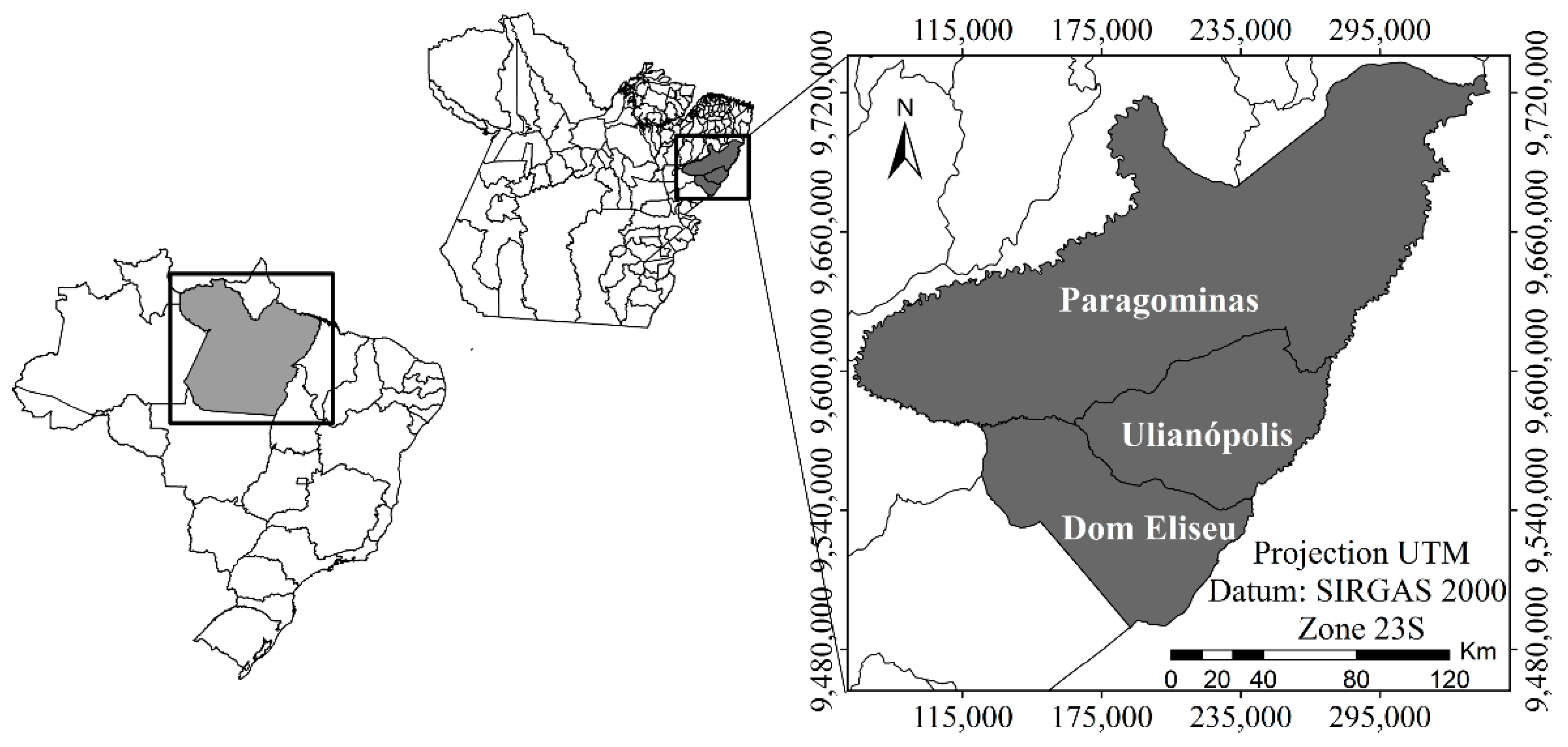
2. Materials and Methods
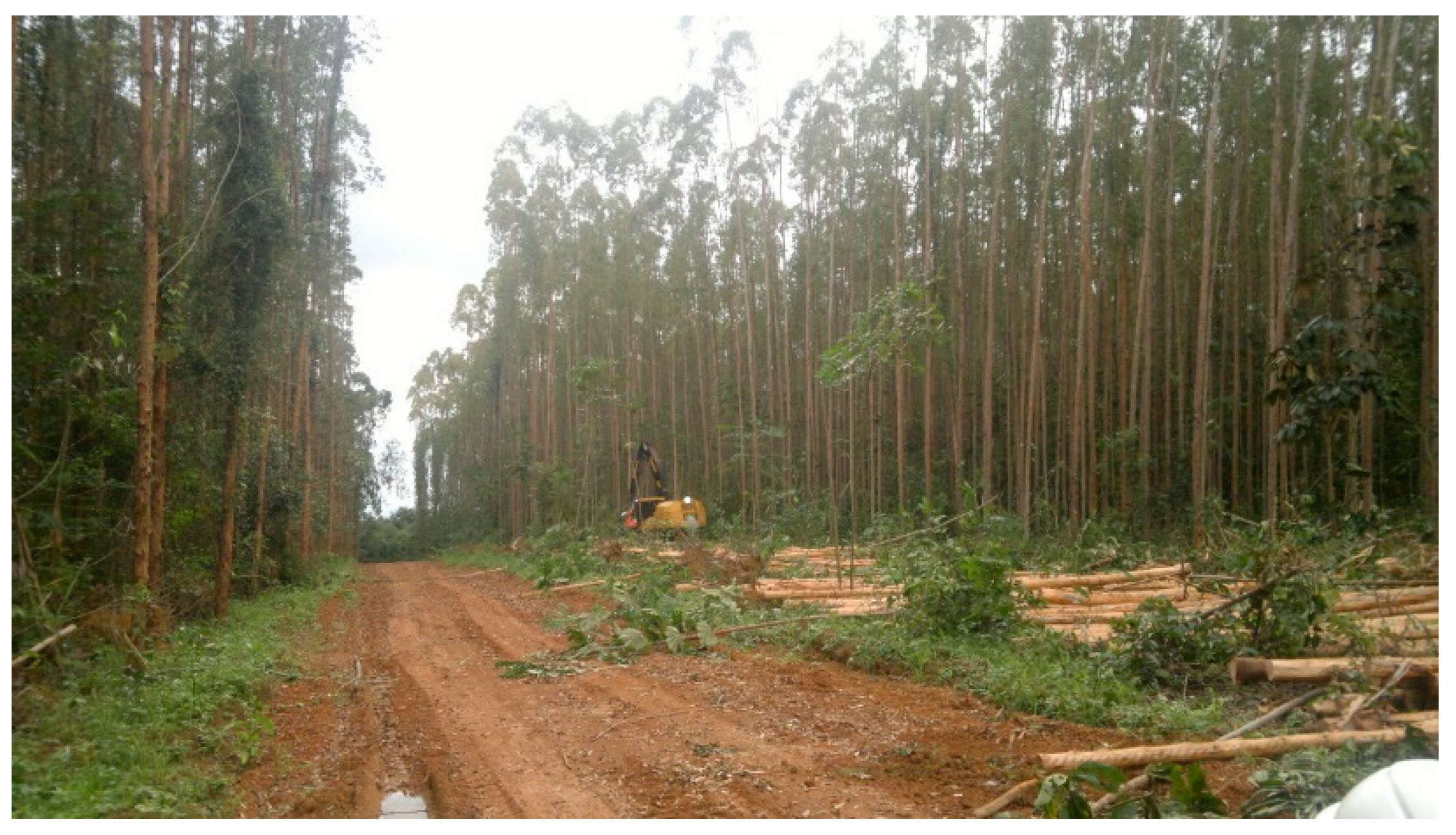
2.1. Data

The research was carried out in clonal Eucalyptus plantations, spaced 3 × 3 m and aged 2–6 years, in the municipalities of Dom Eliseu, Paragominas, and Ulianópolis, mesoregion of Pará State, Brazil (Figure 1). The representation of the Eucalyptus plantations structure can be visualized in Figure 2.
The minimum diameter at breast height (dbh) was 4.15 cm and the maximum was 25.90 cm. Thus, the trees were classified in classes of 2 cm amplitude (Table 1). The minimum volume was 0.0018 m3 and the maximum was 0.6822 m3.

Methods for Estimation of the Tree Attributes

A total of 666 sample trees, from 14 clones of different species and hybrids, were felled in 2010, 2011, 2012, and 2013 (Appendix ATable A1). The felled trees were selected in rectangular plots of 24 × 21 m, allocated in areas of all regions.
The diameter at breast height (dbh) in cm of the trees were measured with a tape measure. After harvesting the sample trees, the total height (h; m) was measured with long tape and the diameter with bark were measured in the positions of height (in meters) equal to 0.0, 0.5, 1.0, 1.3, 2.0, 4.0, and so on every two meters to the diameter with bark equal to 4.0 cm. The real volume with bark up to 4 cm in diameter at the top (v) of felled trees was obtained by the Smalian method [25].

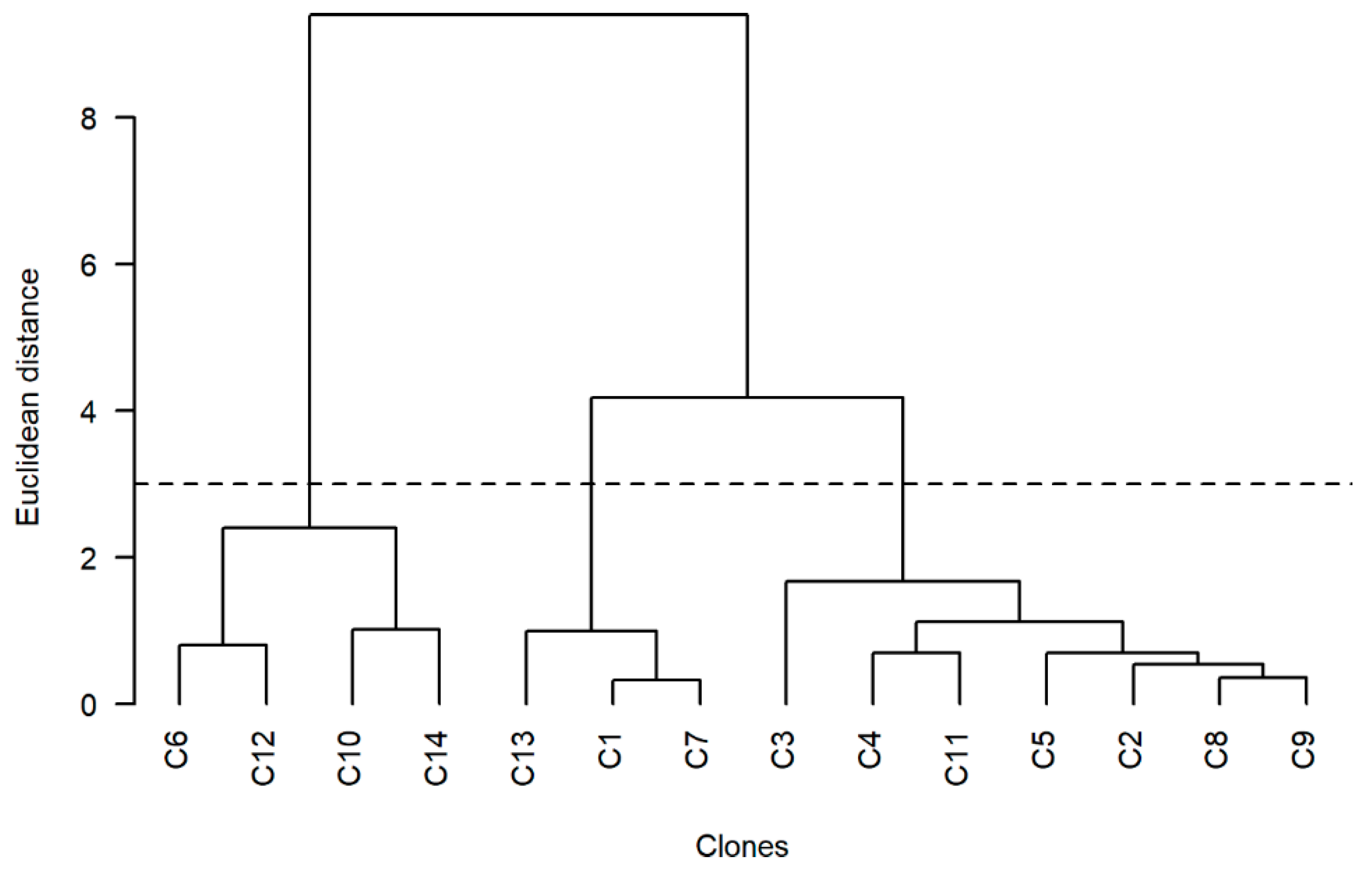
2.2. Clone Cluster Analysis

The cluster analysis was performed to divide the clones into homogeneous groups and allow the comparison between the regression model and ANN in different scenarios. The variables dbh, h, and v (means per clone) were used in the clustering analysis. The Euclidean distance [26], the measure of dissimilarity used to distinguish between groups, and Ward’s method [27], an agglomerative hierarchical technique, were both used to obtain data using the statistics package in R version 3.4.1 (R Core Team, Vienna, Austria).
The efficiency of the grouping method was evaluated with the cophenetic correlation coefficient. A horizontal line between branches was plotted on the resulting dendrogram, forming three groups of clones.

2.3. Settings to Select the Best Model

The 666 trees were used in five statistical models to identify the one with the best fit (Table 2).
The model’s parameters were estimated by the ordinary least squares (OLS) method with the “lm” function in R. The individual volume predicted by logarithmic models was multiplied by the Meyer correction factor [31] [F = e0.5 × MSres] to correct the logarithmic discrepancy, where: F = Meyer correction factor; e = base of natural logarithms; and MSres = mean square of the residuals. The variance inflation factor (VIF) was calculated for models 2, 4, and 5, to verify the presence of multicollinearity in the predictor variables.
The models were compared using the adjusted coefficient of determination (R2adj), residual standard error (Sy.x), variation coefficient (VC%), Student’s t-test for the estimated parameters (5% significance), Akaike’s Information Criterion (AIC), graphical analysis of percentage relative errors (E%) vs. real volumes, and histogram of frequency of E%.

2.4. ANN Training

The trained ANNs were of the multilayer perceptron type (MLP). The typical MLP architecture consists of one input layer containing the predictor variables, one or more hidden layers, and one output layer containing the predicted variable. The layers have a high degree of connectivity, whose strength of the connection is determined by the synaptic weights [32]. In the present study, the ANNs were trained with one hidden layer.
The dbh (cm), h (m), and age (months) were the quantitative input variables, and the region (Dom Eliseu, Paragominas, and Ulianópolis), farm (located in each region), and clone group were the qualitative variables. The clone group was inserted only in the model fit and ANN training with the general data. The number of categories for the qualitative variables varied per scenario, with maximums of 3, 3, and 39 for the region, clone group, and farm, respectively. The v (m3) was the output variable. The activation functions used in training were exponential, identity, logistic, and hyperbolic tangent. The Broyden–Fletcher–Goldfarb–Shanno (BFGS) training algorithm was used. The minimum learning rate was 0.0001, while the maximum was 0.001.
Two hundred ANN were trained by approaches from the two scenarios, totaling 2000 ANN trained. After the training, the five best ANNs were retained per approach based on the correlation coefficient between the real and predicted volumes (r): r = cov(y, ŷ)/[s2(y) × s2(ŷ)]1/2, where: s2 = variance; cov = covariance; y = real commercial volume with bark v (m3), and ŷ = predicted commercial volume with bark v (m3).
The initial ANN weights were randomly generated. The ANNs were obtained with the Neural Networks tool in Statistica 13.2 Trial version (StatSoft Inc., Tulsa, OK, USA).

Selection of the Best ANN

The ANNs retained in the training stage were applied in the generalization dataset and compared to each other by statistics: r, root mean square error in percentage, RMSE% = 100/ӯ × [1/n × ∑(ŷiyi)2]0.5, bias = 1/n × ∑[ŷiyi] and error variance = 1/n × ∑[bias − (ŷiyi)]2. The best network, per approach, was selected using the weighted value method [33]: WV = ∑Nri × Wi, where: WV = weighted value; yi = real commercial volume with bark v (m3); ŷi = predicted commercial volume with bark v (m3); ӯ = average of real volumes (m3); n = total number of observations; Nri = number of records with the ith placement; and Wi = weight of the ith placement.

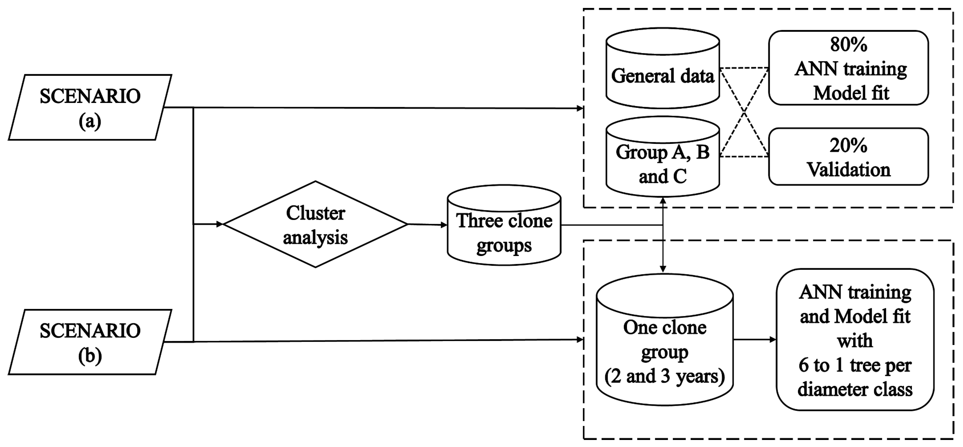
2.5. Experimental Scenarios

The methods were applied and evaluated in two scenarios: (a) the regression model fit and ANN training with 80% of the data (533 trees), and per clone group, after cluster analysis, with 80% of the trees in each group; and (b) model fit and ANN training with trees of only one clone group at the ages of 2 and 3 years, with six, five, four, three, two, and one tree per diameter class as sample intensities (Figure 3).
The datasets for the model fit and ANN training in the two scenarios were randomly selected. The age, in months, was included in the fit of the volumetric model in both scenarios to obtain more accurate predictions.

2.6. Methods Analysis

The analysis of the method predictions (regression and ANN) in both scenarios was based on the statistics cited: r, RMSE%, bias and error variance. Scatter plots of the standardized residuals as a function of the predicted v were plotted using the following equation: sr = ŷiyi/(∑eiē/n − 1)0.5, where sr = standardized residuals; yi = real commercial volume with bark v (m3); ŷi = predicted commercial volume with bark v (m3); ei = difference between the real and predicted volume of the ith tree (m3); ē = mean of the difference between the real and predicted volume (m3); and n = total number of observations.
In scenario (b), an analysis of variance (ANOVA) was performed with a 3 × 5 factorial arrangement: three treatments (regression, ANN, and real) and five sample intensity levels (six to two trees/class) were used to evaluate the differences between the means of the predicted and real values in the sample intensities.
Before ANOVA, the normality of the data was verified with the Lilliefors test and the homogeneity of variance (homoscedasticity) with the Bartlett’s test at the 1% significance level. The “lillie.test” function of the ‘nortest’ package was used in the normality test and the “bartlett.test” function of the statistics package was used in the homoscedasticity test, both in R.

2.7. Methods Validation

The regression and ANN predictions, at the 5% significance level, were tested with the Kolmogorov–Smirnov test [20]. The hypothesis tested was as follows: Hn = the frequency distribution of individuals by volume class was equal, and Ha = the frequency distribution of individuals by volume class was different. This statistic was calculated with the “ks.test” function of the statistics package inside R. The trees used to validate the datasets were those that did not participate in the ANN training and regression fit; thus, biases in the predictions were avoided.

3. Results

3.1. Clone Grouping

In the evaluation of the resulting dendrogram, the cophenetic correlation coefficient was 0.8031, representing good reliability and low distortion in the generation of the dendrogram from the data. The groups formed were named A, B, and C, with v averages of 0.1444, 0.1161, and 0.0758 m3, respectively. The horizontal line intercepted the dendrogram between the two and four Euclidean distances, configuring the following groups of clones: group A formed by clones C2, C3, C4, C5, C8, C9, and C11 (n = 222); B by C1, C7, and C13 (n = 373); and C by C6, C10, C12, and C14 (n = 71) (Figure 4). The union of clones by clustering, with high, medium, and low values of v in groups A, B, and C, respectively, reduced the variability of v within the groups. Due to the greater number of clones and a sufficient number of trees to reduce the sample intensity, clone group A was chosen for the model fit and ANN training in scenario (b) (Table A2).

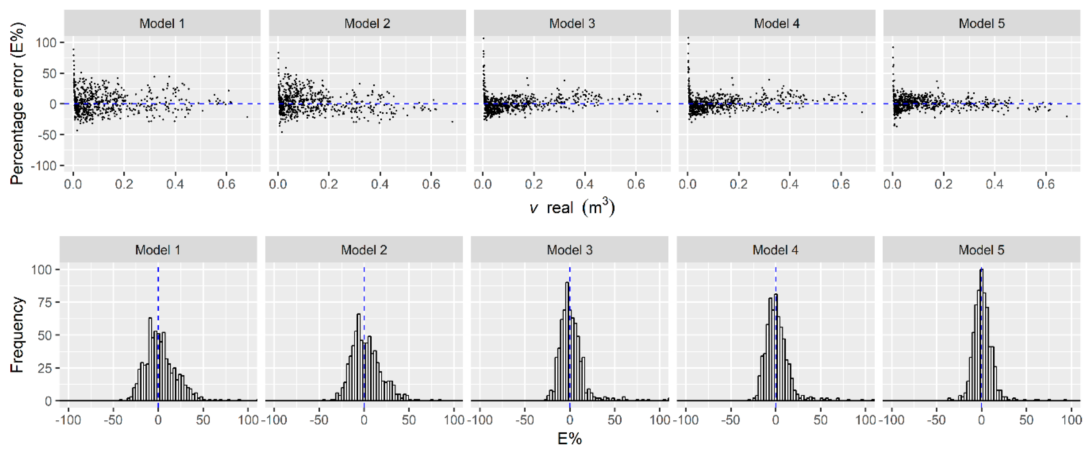
3.2. Best Model Selection

According to the statistical result, the Model 5 (Prodan) presented a higher R2adj value and smaller Sy.x, VC%, and AIC (Table 3). The distribution frequency of E% was more concentrated in the zero value for Model 5. The variation in errors of Model 5 was also smaller than that in the other models, and therefore, this model was selected for evaluation with ANN in the later stages (Figure 5). Models 2 and 5 presented VIF > 10, indicating the presence of multicollinearity.

3.3. ANN Retained in Scenarios (a) and (b)

The selected ANNs presented a high degree of correlation between the predicted and real v in the generalization, with r > 0.9860 (Table 4). The exponential activation function was the most frequent and the identity was the least frequent in the selected ANNs. The neuron number in the hidden layer varied from 3–25 in scenario (a) and from 1–30 in (b). In scenario (a), the number of input variables of ANNs with the general data was higher (22–48) than the other approaches of this same scenario and, in scenario (b), the number of input variables in the intensity of the one tree per diameter class was lower (13–19).

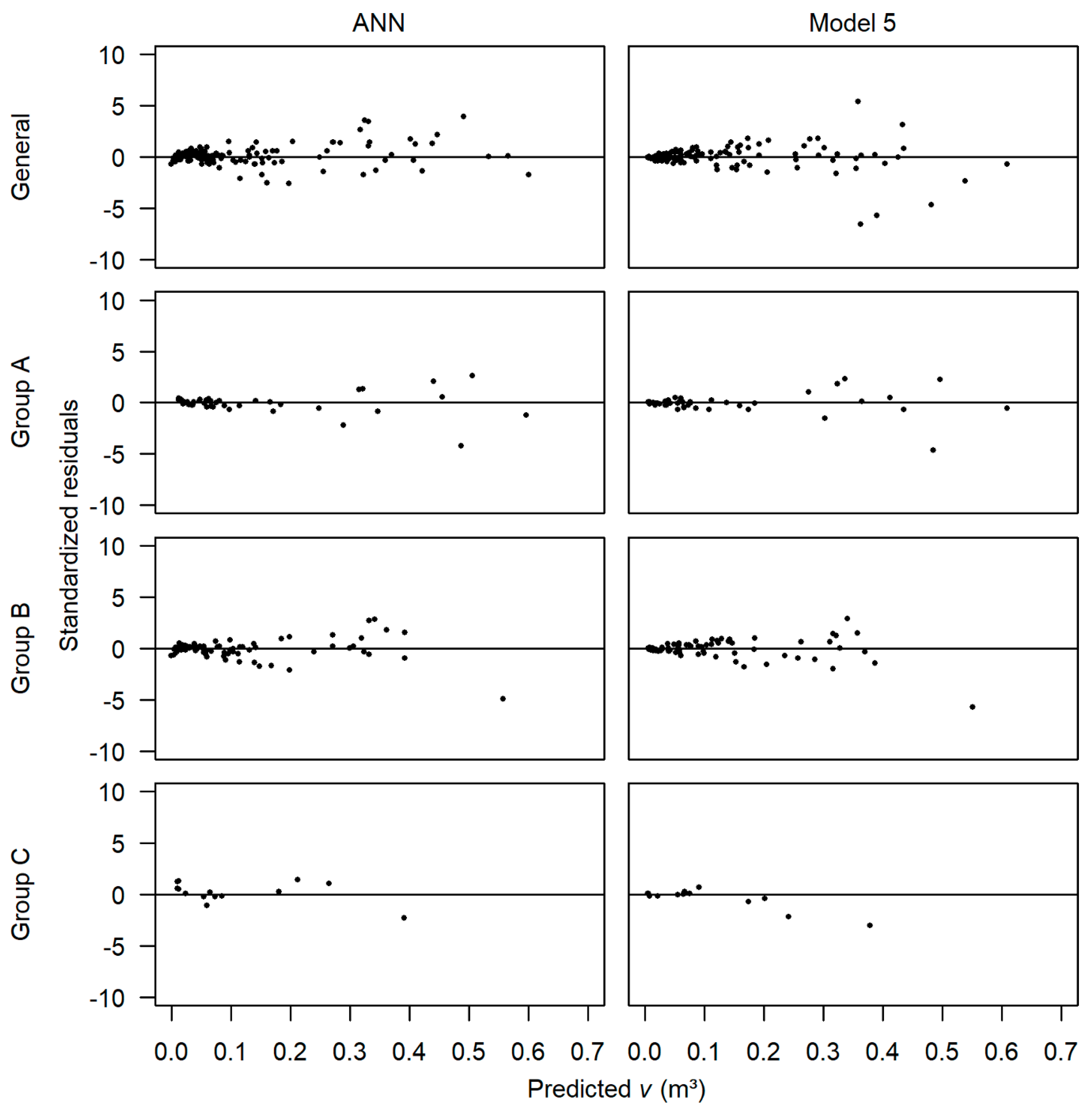
3.4. Predictions Assessment in Scenario (a)

The volume predictions of Model 5 and the best ANN selected for the general data and for each clone group showed a high correlation between real volumes, with r ≥ 0.9940 (Table 5). The ANN was modeled more efficiently in the approach with the general data, with an RMSE smaller than 8%. The error variations of Model 5 in clone groups A and B were smaller than those of ANN. The accuracy in the v predictions of upper classes was lower in both methods (Figure 6).

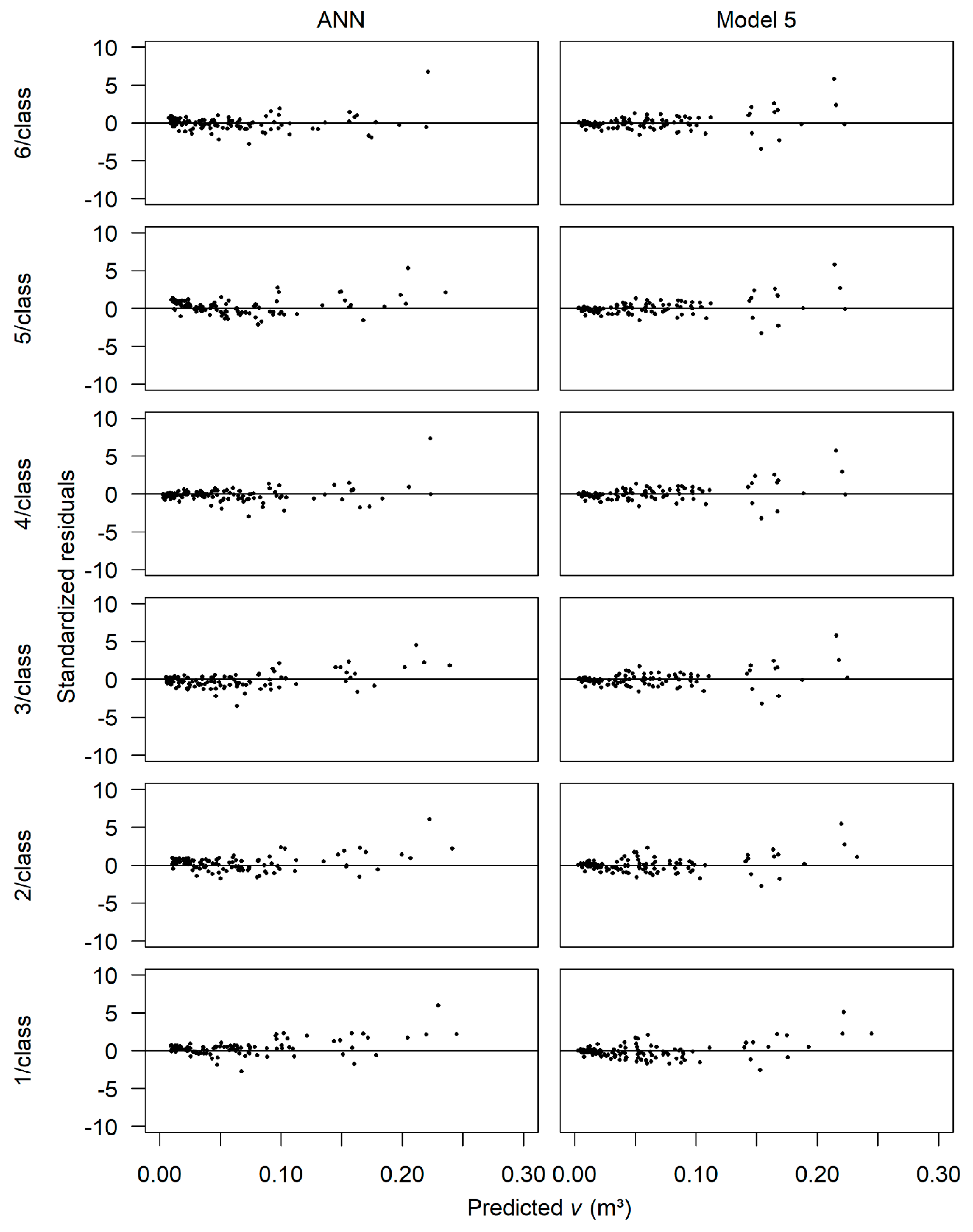
3.5. Predictions Assessment in Scenario (b)

As in scenario (a), the r values in the two methods were relatively high (≥0.9843) (Table 6). The RMSE% values of ANN with five, four, and two trees per class, and of Model 5 with six, three, and one tree per class were smaller. The dispersion of the residuals, for both methods, was more accurate along the zero axis in the smaller and intermediate values of v and less accurate in the larger values (Figure 7).

3.6. Variance Analysis for Means in Scenario (b)

In the normality test, values of v with Model 5 and ANN were significant at 1%, except for the intensity of five and four trees per diameter class, respectively (Table A3). Therefore, the values were transformed into natural logarithms and submitted to a new Lilliefors test. After the transformation, the real and predicted values in the intensities of six to two trees per diameter class presented normality. In the homoscedasticity test, the v values of all sample intensities presented homogeneity of variance, with p-values greater than 0.01. The mean values of v in ANOVA did not differ between treatments and intensities, with Fcal = 0.25 and p-value = 0.98 (Table A4).

3.7. Predictions Validation in Both Scenarios

The predicted v distributions relative to the real values in scenarios (a) and (b) with the Kolmogorov–Smirnov test were similar in both methods (Model 5 and ANN), with p-values greater than 1% (Table A5), thus, the hypothesis Hn was not rejected.

4. Discussion

New methods for predicting timber volume without reducing accuracy are needed to reduce the costs of felling sample trees. ANN has advantages over linear regression models due to factors such as the ability to learn and generalize, noise tolerance, and modeling of non-linear relationships between variables [34,35,36,37]. However, in the present study, it was observed that linear regression may also overcome the ANNs, contrary to other studies [21,38,39]. In addition, regression models are easier to implement and can provide logical estimates under extrapolation [1,40]. Thus, the comparison between the two methods is valid to investigate which is more appropriate for data modeling.
The overestimation of some smaller values of v in the five fitted models (Figure 5) indicated the presence of outliers [41,42,43], however, this did not significantly influence the predictions of the best model. The selection of Model 5 for ANN evaluation was due to the good statistical fit, more compact residual distribution, and lower variability and bias in the predictions. This choice reinforces the importance of testing more than one model per situation, despite the Schumacher–Hall model being reported as the best model to predict tree volume [44,45,46]. Thus, Model 5 best fits the data of this study, being the most suitable to predict commercial volume at the regional level. The presence of multicollinearity was expected for the independent variables of Models 2 and 5. Thus, the models should be used with caution for data coming from different locations and differing from the range of variables presented in this study.
The high r of ANN retained in both scenarios was due to their ability to model complex relationships between qualitative and quantitative variables [47,48,49]. The largest neuron number in the hidden layer for the general data was due to the modeling complexity with qualitative variables (region, farm, and groups of clones) [50]. The input number reduction in ANN up to the one tree per class intensity was due to data randomization without the inclusion of some categories of qualitative variables in the training (region and farm). According to Silva et al. [51], obtaining the appropriate architecture of the neural network is optimized by successive attempts that produce satisfactory results. Görgens et al. [15] argue that architecture is directly related to the learning power of the network, and, in more complex data, the demand for neurons and even for layers increases. In the present study, the non-linear behavior of the data required the use of more complex variables, and, therefore, influenced the number of neurons in the input and hidden layers. Thus, it is important to test as many architectures as possible to find the best fit for the data distribution.
Analyzing scenario (a), the highest r value and lowest RMSE% of the ANN, with the general data, indicate that the precision increases with the inclusion of the clone group as a qualitative variable [22,23,52]. The smaller error variations in the equations with Model 5 in the predictions per clone group are necessary to reduce the data variability by stratification, generating an equation per clone group. Similar results were obtained by Ribeiro et al. [23] using the Schumacher-Hall model and ANNs for estimation of the bole volume for different species in the Tapajós National Forest. After stratifying the data for the regression, they observed an improvement in the parameter estimates in comparison to the use of a single equation. The need to generate an equation per approach requires more time for data collection and fit [23] and, therefore, v can be predicted with an ANN for the general data. The smaller precision in the upper classes of v for the approach of both methods in scenario (a) was due to the greater data variation in these classes.
The high r value in scenario (b) indicates a good fit of the methods in predicting the data. The highest r value and lowest RMSE% of the equations with Model 5 compared to ANN in the intensities of six and three trees per class suggested that a greater number of trees decreased the quadratic error and increased the accuracy of the predictions. For Model 5, at least three trees per class are better for predicting v, while for ANN, at least four trees per class are better for prediction, based on the increase in RMSE% in the intensities of two and three trees per class, respectively. This result was similar to that found by David et al. [53], in which they affirmed that it is possible to predict stem volume of Eucalyptus grandis W. Hill ex Maiden × Eucalyptus urophylla ST Blake by measuring at least two trees per class. However, these authors used sampling proportional to the frequency of trees by diameter class; the present study used the same number of trees per class, except for the intensity with only one tree in the class.
The mean similarities of v in ANOVA between treatments and intensities of six to two trees per diameter class indicates that the reduction in the number of trees did not significantly decrease the accuracy of the estimates. The reduction in the sampling intensity may be feasible for the prediction of v, representing time and cost savings in the collection of volume data [17]. The increase in the error for volume prediction using one tree per diameter class indicates the difficulty in this sampling to represent all variations in the data. Therefore, further studies on volume estimation at different sample intensities can be performed locally or regionally in order to verify the gains in the optimization of the sampling and in the precision and accuracy of the estimates. In addition, tests of parameterization of ANNs and evaluation of possible gain by changing the algorithm to others such as the resilient propagation, backpropagation, and Levenberg-Marquardt, as well as normalization and equalization tests can bring better results when estimating commercial volume [23].
Concerning the Kolmogorov-Smirnov test, the similarities in the predicted v distribution relative to the real values indicated ANN and Model 5 as the most appropriate methods to predict timber volume of Eucalyptus clones at the tested sample intensities due to the accuracy [20]. The v distribution with the trend of real data, even with their complexity, resulted in a good quality fit for Model 5.

5. Conclusions

The ANN and linear regression proved to be efficient in predicting commercial volume in scenarios (a) and (b). The ANN more efficiently predicted data at more general levels (all clone groups). Model 5 (Prodan) also generated predictions with accuracy, and, among the regression models, was the best fit to the data.
The volume with bark up to 4 cm in diameter at the top of Eucalyptus clones in the southeast mesoregion of Pará State, Brazil, can be predicted with at least three sample trees per diameter class by regression and four trees per class by ANN.
In addition to the accuracy of the estimates using ANN and the model of Prodan, their performance in predicting volume using smaller samples represents costs and time reduction for forest inventory practices.

Author Contributions

Conceptualization, I.d.S.T.J. and J.E.C.d.R.; Formal analysis, I.d.S.T.J. and J.E.C.d.R.; Methodology, I.d.S.T.J. and J.E.C.d.R.; Resources, A.d.S.C.; Writing—original draft, I.d.S.T.J., J.E.C.d.R., J.C.Z. and H.G.L.; Writing—review and editing, I.d.S.T.J., J.E.C.d.R., Â.A.E., A.d.S.C., J.C.Z., A.A.F. and H.G.L.

Funding

This research was funded by CNPq (Conselho Nacional de Desenvolvimento Científico e Tecnológico) (Process: 134604/2017-2).

Acknowledgments

We thank the “Conselho Nacional de Desenvolvimento Científico e Tecnológico (CNPq)”, “Coordenação de Aperfeiçoamento de Pessoal de Nível Superior (CAPES)” and the “Fundação de Apoio à Pesquisa do Estado de Minas Gerais (FAPEMIG)” for their financial support, and DAP Engenharia Florestal Ltda. for operationally supporting this work.

Conflicts of Interest

The authors declare that they have no conflict of interest.

Appendix A

Table A1. Description of species and hybrids for each clone of Eucalyptus.
CloneSpecies/Hybridn
C1Eucalyptus grandis W. Hill ex Maiden × Eucalyptus urophylla S.T. Blake339
C2Eucalyptus grandis W. Hill ex Maiden × Eucalyptus urophylla S.T. Blake42
C3Eucalyptus grandis W. Hill ex Maiden × Eucalyptus urophylla S.T. Blake113
C4Eucalyptus grandis W. Hill ex Maiden43
C5Eucalyptus platyphylla F. Muell.2
C6Eucalyptus platyphylla F. Muell.2
C7Eucalyptus grandis W. Hill ex Maiden × Eucalyptus urophylla S.T. Blake2
C8Eucalyptus grandis W. Hill ex Maiden × Eucalyptus urophylla S.T. Blake2
C9Eucalyptus grandis W. Hill ex Maiden × Eucalyptus urophylla S.T. Blake13
C10Eucalyptus urophylla S.T. Blake11
C11Eucalyptus urophylla S.T. Blake7
C12Eucalyptus urophylla S.T. Blake54
C13Eucalyptus urophylla S.T. Blake32
C14Eucalyptus camaldulensis Dehnh. × Eucalyptus urophylla S.T. Blake4
Total 666
n = number of observations.
Table A2. Number of trees (n) per diametric class in clone A group at two and three years of age, simultaneously.
dbh Class (cm)n
4–623
6–828
8–1028
10–1227
12–1421
14–1613
16–1810
18–201
Total151
Table A3. Summary of the Lilliefors (normality) and Bartlett’s (homoscedasticity) tests for the real and predicted values in the different sample intensities of scenario (b).
Intensity SampleTreatmentnOriginal ValueTransformed Value
Lillieforsp-ValueBartlettp-ValueLillieforsp-Value
Real1080.13486 *0.00005 0.07881 ns>0.01
6/classANN1080.15964 *0.000380.14973 ns>0.010.07341 ns>0.01
Model 51080.14441 *0.008610.08355 ns>0.01
5/classANN1080.16288 *0.000190.21673 ns>0.010.07269 ns>0.01
Model 51080.14355 ns>0.010.09035 ns>0.01
4/classANN1080.14298 ns>0.010.21918 ns>0.010.08726 ns>0.01
Model 51080.14409 *0.009170.08969 ns>0.01
3/classANN1080.16724 *0.000070.40207 ns>0.010.07236 ns>0.01
Model 51080.14370 *0.009890.08892 ns>0.01
2/classANN1080.16676 *0.000080.16563 ns>0.010.06155 ns>0.01
Model 51080.14492 *0.007810.09548 ns>0.01
1/classANN1080.16423 *0.000140.46086 ns>0.010.06843 ns>0.01
Model 51080.15562 *0.000900.10664 *0.00416
* significant value; ns non-significant value; n = number of observations.
Table A4. Analysis of variance (ANOVA) of the means of the real and predicted values by ANN and regressions with Model 5 at sample intensities of six to two trees per diameter class in scenario (b).
Source of VariancedfSSMSFcal
Treatments20.60.2930.303 ns
Intensities41.20.2950.305 ns
Treatments × Intensities820.2460.254 ns
Residuals16051549.80.966
Total16191553.6
ns non-significant value (p > 0.05).
Table A5. Results of the Kolmogorov–Smirnov test calculated (Dcal) for validation of the predicted values by ANN and equations with Model 5 in all approaches to scenarios (a) and (b).
ScenarioApproachnANNModel 5
Dcalp-ValueDcalp-Value
AGeneral1330.0526 ns>0.010.0376 ns>0.01
AGroup A440.1136 ns>0.010.0682 ns>0.01
AGroup B740.0405 ns>0.010.0541 ns>0.01
AGroup C140.2857 ns>0.010.1429 ns>0.01
B6/class1080.0648 ns>0.010.0556 ns>0.01
B5/class1080.1389 ns>0.010.0648 ns>0.01
B4/class1080.0556 ns>0.010.0648 ns>0.01
B3/class1080.0648 ns>0.010.0463 ns>0.01
B2/class1080.1389 ns>0.010.0556 ns>0.01
B1/class1080.1111 ns>0.010.0648 ns>0.01
ns non-significant value; n = number of observations.

References

  1. Ferraz Filho, A.C.; Mola-Yudego, B.; Ribeiro, A.; Scolforo, J.R.S.; Loos, R.A.; Scolforo, H.F. Height-diameter models for eucalyptus sp. plantations in Brazil. Cerne 2018, 24, 9–17. [Google Scholar] [CrossRef]
  2. Binkley, D.; Campoe, O.C.; Alvares, C.; Carneiro, R.L.; Cegatta, I.; Stape, J.L. The interactions of climate, spacing and genetics on clonal Eucalyptus plantations across Brazil and Uruguay. For. Ecol. Manag. 2017, 405, 271–283. [Google Scholar] [CrossRef]
  3. Dasgupta, M.G.; Dharanishanthi, V. Identification of PEG-induced water stress responsive transcripts using co-expression network in Eucalyptus grandis. Gene 2017, 627, 393–407. [Google Scholar] [CrossRef] [PubMed]
  4. Rocha, J.E.C.; Brasil Neto, A.B.; Noronha, N.C.; Gama, M.A.P.; Carvalho, E.J.M.; Silva, A.R.; Santos, C.R.C. Organic matter and physical-hydric quality of an oxisol under eucalypt planting and abandoned pasture. Cerne 2016, 22, 381–388. [Google Scholar] [CrossRef]
  5. Santana, R.C.; Barros, N.F.; Leite, H.G.; Comerford, N.B.; Novais, R.F. Estimativa de biomassa de plantios de eucalipto no Brasil. Rev. Árvore 2008, 32, 697–706. [Google Scholar] [CrossRef] [Green Version]
  6. Matos, G.S.B.; Silva, G.R.; Gama, M.A.P.; Vale, R.S.; Rocha, J.E.C. Desenvolvimento inicial e estado nutricional de clones de eucalipto no nordeste do Pará. Acta Amazon. 2012, 42, 491–500. [Google Scholar] [CrossRef]
  7. Ounban, W.; Puangchit, L.; Diloksumpun, S. Development of general biomass allometric equations for Tectona grandis Linn.f. and Eucalyptus camaldulensis Dehnh. plantations in Thailand. Agric. Nat. Resour. 2016, 50, 48–53. [Google Scholar] [CrossRef]
  8. Paul, K.I.; Roxburgh, S.H.; Chave, J.; England, J.R.; Zerihun, A.; Specht, A.; Lewis, T.; Bennett, L.T.; Baker, T.G.; Adams, M.A.; et al. Testing the generality of above-ground biomass allometry across plant functional types at the continent scale. Glob. Chang. Biol. 2016, 22, 2106–2124. [Google Scholar] [CrossRef]
  9. Forrester, D.I.; Tachauer, I.H.H.; Annighoefer, P.; Barbeito, I.; Pretzsch, H.; Ruiz-Peinado, R.; Stark, H.; Vacchiano, G.; Zlatanov, T.; Chakraborty, T.; et al. Generalized biomass and leaf area allometric equations for European tree species incorporating stand structure, tree age and climate. For. Ecol. Manag. 2017, 396, 160–175. [Google Scholar] [CrossRef]
  10. Fortier, J.; Truax, B.; Gagnon, D.; Lambert, F. Allometric equations for estimating compartment biomass and stem volume in mature hybrid poplars: General or site-specific? Forests 2017, 8, 309. [Google Scholar] [CrossRef]
  11. García-Espinoza, G.G.; Aguirre-Calderón, O.A.; Quiñonez-Barraza, G.; Alanís-Rodríguez, E.; De Los Santos-Posadas, H.M.; García-Magaña, J.J. Taper and volume systems based on ratio equations for Pinus pseudostrobus Lindl. in Mexico. Forests 2018, 9, 344. [Google Scholar] [CrossRef]
  12. IBÁ. INDÚSTRIA BRASILEIRA DE ÁRVORES. Report IBÁ-2017. Indicators of Performance of the National Sector of Planted Trees for the Year 2016. Available online: http://iba.org/images/shared/Biblioteca/IBA_RelatorioAnual2017.pdf (accessed on 10 August 2018).
  13. Cosenza, D.N.; Leite, H.G.; Marcatti, G.E.; Binoti, D.H.B.; Alcântara, A.E.M.; Rode, R. Classificação da capacidade produtiva de sítios florestais utilizando máquina de vetor de suporte e rede neural artificial. Sci. For. 2015, 43, 955–963. [Google Scholar] [CrossRef]
  14. Zhang, D.; Zhang, L.; Ye, Q.; Ruan, H. Robust learning-based prediction for timber-volume of living trees. Comput. Electron. Agric. 2017, 136, 97–110. [Google Scholar] [CrossRef]
  15. Görgens, E.B.; Leite, H.G.; Gleriani, J.M.; Soares, C.P.B.; Ceolin, A. Influência da arquitetura na estimativa de volume de árvores individuais por meio de redes neurais artificiais. Rev. Árvore 2014, 38, 289–295. [Google Scholar] [CrossRef] [Green Version]
  16. Görgens, E.B.; Leite, H.G.; Santos, H.N.; Gleriani, J.M. Estimação do volume de árvores utilizando redes neurais artificiais. Rev. Árvore 2009, 33, 1141–1147. [Google Scholar] [CrossRef] [Green Version]
  17. Binoti, M.L.M.S.; Binoti, D.H.B.; Leite, H.G.; Garcia, S.L.R.; Ferreira, M.Z.; Rode, R.; Silva, A.A.L. Redes neurais artificiais para estimação do volume de árvores. Rev. Árvore 2014, 38, 283–288. [Google Scholar] [CrossRef] [Green Version]
  18. Cosenza, D.N.; Soares, A.A.V.; de Alcântara, A.E.M.; da Silva, A.A.L.; Rode, R.; Soares, V.P.; Leite, H.G. Site classification for eucalypt stands using artificial neural network based on environmental and management features. Cerne 2017, 23, 310–320. [Google Scholar] [CrossRef]
  19. Özçelik, R.; Diamantopoulou, M.J.; Crecente-Campo, F.; Eler, U. Estimating Crimean juniper tree height using nonlinear regression and artificial neural network models. For. Ecol. Manag. 2013, 306, 52–60. [Google Scholar] [CrossRef]
  20. Diamantopoulou, M.J.; Özçelik, R.; Crecente-Campo, F.; Eler, Ü. Estimation of Weibull function parameters for modelling tree diameter distribution using least squares and artificial neural networks methods. Biosyst. Eng. 2015, 133, 33–45. [Google Scholar] [CrossRef]
  21. Vahedi, A.A. Artificial neural network application in comparison with modeling allometric equations for predicting above-ground biomass in the Hyrcanian mixed-beech forests of Iran. Biomass Bioenergy 2016, 88, 66–76. [Google Scholar] [CrossRef]
  22. Reis, L.P.; Souza, A.L.; Mazzei, L.; Reis, P.C.M.; Leite, H.G.; Soares, C.P.B.; Torres, C.M.M.E.; Silva, L.F.; Ruschel, A.R. Prognosis on the diameter of individual trees on the eastern region of the amazon using artificial neural networks. For. Ecol. Manag. 2016, 382, 161–167. [Google Scholar] [CrossRef]
  23. Ribeiro, R.B.S.; Gama, J.R.V.; Souza, A.L.; Leite, H.G.; Soares, C.P.B.; Silva, G.F. Métodos para estimar o volume de fustes e galhos na Floresta Nacional do Tapajós. Rev. Árvore 2016, 40, 81–88. [Google Scholar] [CrossRef]
  24. Rocha, S.J.S.S.; Torres, C.M.M.E.; Jacovine, L.A.G.; Leite, H.G.; Gelcer, E.M.; Neves, K.M.; Schettini, B.L.S.; Villanova, P.H.; da Silva, L.F.; Reis, L.P.; et al. Artificial neural networks: Modeling tree survival and mortality in the Atlantic Forest biome in Brazil. Sci. Total Environ. 2018, 645, 655–661. [Google Scholar] [CrossRef] [PubMed]
  25. Husch, B.; Beers, T.W.; Kershaw, J.A., Jr. Forest Mensuration, 4th ed.; John Wiley & Sons: Hoboken, NJ, USA, 2003; 443p. [Google Scholar]
  26. Mesquita, D.P.P.; Gomes, J.P.P.; Souza Junior, A.H.; Nobre, J.S. Euclidean distance estimation in incomplete datasets. Neurocomputing 2017, 248, 11–18. [Google Scholar] [CrossRef]
  27. Ward, J.H., Jr. Hierarchical grouping to optimize an objective function. J. Am. Stat. Assoc. 1963, 58, 236–244. [Google Scholar] [CrossRef]
  28. Camolesi, J.F.; Scolforo, J.R.S.; Oliveira, A.D.; Acerbi Júnior, F.W.; Rufini, A.L.; Mello, J.M. Ajuste, seleção e teste de identidade de modelo para volume e número de moirões da candeia (Eremanthus erythropappus). Cerne 2010, 16, 431–441. [Google Scholar] [CrossRef]
  29. Schneider, P.R.; Tonini, H. Utilização de variáveis dummy em equações de volume para Acacia mearnsii De Wild. Ciênc. Florest. 2003, 13, 121–129. [Google Scholar] [CrossRef]
  30. Rolim, S.G.; Couto, H.T.Z.; Jesus, R.M.; França, J.T. Modelos volumétricos para a Floresta Nacional do Tapirapé-Aquirí, Serra dos Carajás (PA). Acta Amazon. 2006, 36, 107–114. [Google Scholar] [CrossRef]
  31. Meyer, H.A. A Correction for a Systematic Error Occurring in the Application of the Logarithmic Volume Equation; Forestry School Research: Scranton, PA, USA, 1941; 15p.
  32. Haykin, S. Neural Networks and Learning Machines; Pearson: Hoboken, NJ, USA, 2009; ISBN 9780131471399. [Google Scholar]
  33. Thomas, C.; Andrade, C.M.; Schneider, P.R.; Finger, C.A.G. Comparação de equações volumétricas ajustadas com dados de cubagem e análise de tronco. Ciênc. Florest. 2006, 16, 319–327. [Google Scholar] [CrossRef]
  34. Lek, S.; Guégan, J.F. Artificial neural networks as a tool in ecological modelling, an introduction. Ecol. Model. 1999, 120, 65–73. [Google Scholar] [CrossRef]
  35. Diamantopoulou, M.J. Artificial neural networks as an alternative tool in pine bark volume estimation. Comput. Electron. Agric. 2005, 48, 235–244. [Google Scholar] [CrossRef]
  36. Che, S.; Tan, X.; Xiang, C.; Sun, J.; Hu, X.; Zhang, X.; Duan, A.; Zhang, J. Stand basal area modelling for Chinese fir plantations using an artificial neural network model. J. For. Res. 2018. [Google Scholar] [CrossRef]
  37. Reis, L.P.; Souza, A.L.; Reis, P.C.M.; Mazzei, L.; Soares, C.P.B.; Torres, C.M.M.E.; Silva, L.F.; Ruschel, A.R.; Rêgo, L.J.S. Estimation of mortality and survival of individual trees after harvesting wood using artificial neural networks in the amazon rain forest. Ecol. Eng. 2018, 112, 140–147. [Google Scholar] [CrossRef]
  38. Diamantopoulou, M.J. Assessing a reliable modeling approach of features of trees through neural network models for sustainable forests. Sustain. Comput. Inform. Syst. 2012, 2, 190–197. [Google Scholar] [CrossRef]
  39. Soares, F.A.A.M.N.; Flôres, E.L.; Cabacinha, C.D.; Carrijo, G.A.; Veiga, A.C.P. Recursive diameter prediction and volume calculation of eucalyptus trees using Multilayer Perceptron Networks. Comput. Electron. Agric. 2011, 78, 19–27. [Google Scholar] [CrossRef]
  40. Sabatia, C.O.; Burkhart, H.E. Predicting site index of plantation loblolly pine from biophysical variables. For. Ecol. Manag. 2014, 326, 142–156. [Google Scholar] [CrossRef]
  41. Ebling, Â.A.; Péllico Netto, S. Modelagem de ocorrência de coortes na estrutura diamétrica da Araucaria angustifolia (Bertol.) Kuntze. Cerne 2015, 21, 251–257. [Google Scholar] [CrossRef]
  42. Campos, J.C.C.; Leite, H.G. Mensuração Florestal: Perguntas e Respostas, 4rd ed.; Editora UFV: Viçosa, Brazil, 2013; pp. 491–493. ISBN 978-85-7269-465-0. [Google Scholar]
  43. Cysneiros, V.C.; Pelissari, A.L.; Machado, S.A.; Figueiredo Filho, A.; Souza, L. Modelos genéricos e específicos para estimativa do volume comercial em uma floresta sob concessão na Amazônia. Sci. For. 2017, 45, 295–304. [Google Scholar] [CrossRef]
  44. Návar, J.; Ríos-Saucedo, J.; Pérez-Verdín, G.; Rodríguez-Flores, F.J.; Domínguez-Calleros, P.A. Regional aboveground biomass equations for North American arid and semi-arid forests. J. Arid Environ. 2013, 97, 127–135. [Google Scholar] [CrossRef]
  45. Sales, F.C.V.; Silva, J.A.A.; Ferreira, R.L.C.; Gadelha, F.H.L. Ajustes de modelos volumétricos para o clone Eucalyptus grandis x E. urophylla cultivados no agreste de Pernambuco. Floresta 2015, 45, 663–670. [Google Scholar] [CrossRef]
  46. Gimenez, B.O.; Santos, L.T.; Gebara, J.; Celes, C.H.S.; Durgante, F.M.; Lima, A.J.N.; Santos, J.; Higuchi, N. Tree climbing techniques and volume equations for Eschweilera (Matá-Matá), a hyperdominant genus in the Amazon forest. Forests 2017, 8, 154. [Google Scholar] [CrossRef]
  47. Özçelik, R.; Diamantopoulou, M.J.; Brooks, J.R.; Wiant Junior, H. Estimating tree bole volume using artificial neural network models for four species in Turkey. J. Environ. Manag. 2010, 91, 742–753. [Google Scholar] [CrossRef]
  48. Nunes, M.H.; Görgens, E.B. Artificial intelligence procedures for tree taper estimation within a complex vegetation mosaic in Brazil. PLoS ONE 2016, 11. [Google Scholar] [CrossRef]
  49. Vahedi, A.A. Monitoring soil carbon pool in the Hyrcanian coastal plain forest of Iran: Artificial neural network application in comparison with developing traditional models. Catena 2017, 152, 182–189. [Google Scholar] [CrossRef]
  50. Diamantopoulou, M.J.; Milios, E. Modelling total volume of dominant pine trees in reforestations via multivariate analysis and artificial neural network models. Biosyst. Eng. 2010, 105, 306–315. [Google Scholar] [CrossRef]
  51. Silva, M.L.M.; Binoti, D.H.B.; Gleriani, J.M.; Leite, H.G. Ajuste do modelo de Schumacher e Hall e aplicação de redes neurais artificiais para estimar volume de árvores de eucalipto. Rev. Árvore 2009, 33, 1133–1139. [Google Scholar] [CrossRef] [Green Version]
  52. Bhering, L.L.; Cruz, C.D.; Peixoto, L.A.; Rosado, A.M.; Laviola, B.G.; Nascimento, M. Application of neural networks to predict volume in eucalyptus. Crop Breed. Appl. Biotechnol. 2015, 15, 125–131. [Google Scholar] [CrossRef] [Green Version]
  53. David, H.C.; Otávio, R.; Miranda, V.; Welker, J.; Fiorentin, L.D.; Ebling, Â.A.; Henrique, P.; Martins, B.; Silva, D. Strategies for stem measurement sampling: A statistical approach of modelling individual tree volume. Cerne 2016, 22, 249–260. [Google Scholar] [CrossRef]
Figure 1. Location of the municipalities of Dom Eliseu, Paragominas, and Ulianópolis, southeast mesoregion of the Pará state, Brazil, generated with ArcGIS 10.4.1 software.
Forests 10 00268 g001
Figure 2. Image of the structure of Eucalyptus plantations in the study area.
Forests 10 00268 g002
Figure 3. Scheme of the approaches used in scenarios (a) and (b). ANN: artificial neural networks.
Forests 10 00268 g003
Figure 4. Dendrogram of the cluster analysis using Ward’s method and the Euclidean distance with interception of the branches by the horizontal dashed line for the formation of clusters with Eucalyptus clones: group A: C3, C4, C11, C5, C2, C8, and C9; group B: C13, C1, and C7; and group C: C6, C12, C10, and C14.
Forests 10 00268 g004
Figure 5. Percentage error vs. real commercial volume with bark up to 4 cm in diameter at the tree top (v) and frequency histogram of E% of the fitted models.
Forests 10 00268 g005
Figure 6. Dispersion of the standardized residuals as a function of the predicted commercial volume with bark up to 4 cm in diameter at the tree top (v), in the sample intensities of scenario (a).
Forests 10 00268 g006
Figure 7. Dispersion of the standardized residuals as a function of the predicted commercial volume with bark up to 4 cm in diameter at the tree top (v), in the sample intensities of scenario (b).
Forests 10 00268 g007
Table 1. Number of trees (n) and mean (and standard deviation) of diameter at breast height (dbh), h, and v per diameter class.
dbh Class (cm)ndbh (cm)h (m)v (m3)
4–6855.09 (0.50)9.23 (1.19)0.0069 (0.0028)
6–8876.86 (0.48)11.46 (1.42)0.0185 (0.0047)
8–10908.99 (0.54)13.35 (2.02)0.0381 (0.0090)
10–129210.77 (0.54)14.86 (2.00)0.0617 (0.0126)
12–148612.83 (0.54)17.04 (2.09)0.0995 (0.0199)
14–167114.95 (0.56)19.02 (1.88)0.1492 (0.0236)
16–185516.83 (0.53)21.56 (2.70)0.2155 (0.0432)
18–203518.92 (0.61)24.92 (1.96)0.3203 (0.0451)
20–223520.83 (0.68)26.23 (2.32)0.3804 (0.0570)
22–242222.95 (0.63)26.20 (2.34)0.4671 (0.0864)
24–26824.54 (0.58)29.53 (1.40)0.5929 (0.0257)
Table 2. Volumetric models tested to predict volume with bark up to 4 cm in diameter at the top of Eucalyptus clone trees.
No.Author *Model
1HuschLn(v) = β0 + β1Ln(dbh) + εi
2BrenacLn(v) = β0 + β1Ln(dbh) + β2dbh−1 + εi
3SpurrLn(v) = β0 + β1Ln(dbh2h) + εi
4Schumacher-HallLn(v) = β0 + β1Ln(dbh) + β2Ln(h) + εi
5ProdanLn(v) = β0 + β1Ln(dbh) + β2Ln2(dbh) + β3Ln(h) + β4Ln2(h) + εi
Ln = natural logarithm; βi = model parameters, where i: 0, 1, 2, 3, and 4; v = commercial volume with bark up to 4 cm in diameter at the top of the tree; h = total height (m); dbh = diameter at breast height (cm); and εi ~ N (0, σ2) = random error; * Models found in: Camolesi et al. [28]; Schneider and Tonini [29]; and Rolim et al. [30].
Table 3. Adjusted coefficient of determination (R2adj), residual standard error (Sy.x, in m3), variation coefficient (VC%), Akaike’s Information Criterion (AIC), and parameters estimated (and standard errors) with significance in the t-test for the fitted models.
Model No.R2adjSy.xVC%AICEstimated Parameters
β0β1β2β3β4
10.95820.0277323.39−439.13−9.606008 *
(±0.0361)
2.855458 *
(±0.0148)
20.96420.0256821.64−509.33−7.834555 *
(±0.2062)
2.329743 *
(±0.0620)
−5.061533 *
(±0.5809)
30.97770.0202817.10−742.82−10.67147 *
(±0.0330)
1.049066 *
(±0.0043)
40.97710.0205517.32−756.89−10.50457 *
(±0.0527)
2.227204 *
(±0.0332)
0.875632 *
(±0.0433)
50.98940.0139511.74−1051.54−10.39049 *
(±0.2743)
4.890782 *
(±0.1599)
−0.598349 *
(±0.0352)
−1.508759 *
(±0.2963)
0.471110 *
(±0.0551)
* p-value < 0.05.
Table 4. Configurations, correlation coefficients between real and predicted values (r), and weighted value (WV) of the best artificial neural network in the generalization of the approaches in scenarios (a) and (b).
ScenarioApproachNetworkNeurons 1rActivation FunctionWV
HL 2OL 3
AGeneralANN 248–25–10.9977ExponentialH. tangent 45
AGroup AANN 530–3–10.9940LogisticLogistic5
AGroup BANN 536–9–10.9955H. tangentIdentity4
AGroup CANN 222–3–10.9992ExponentialExponential6
B6/classANN 519–30–10.9901H. tangentExponential5
B5/classANN 118–12–10.9933ExponentialLogistic8
B4/classANN 317–1–10.9912LogisticIdentity5
B3/classANN 316–9–10.9888ExponentialExponential7
B2/classANN 215–4–10.9880ExponentialExponential7
B1/classANN 513–1–10.9861ExponentialExponential6
1 Number of neurons per layer; 2 Hidden layer; 3 Output layer; 4 Hyperbolic tangent.
Table 5. Correlation coefficient (r), root mean square error (RMSE%), bias, and error variance (EV) of the artificial neural networks and equations with Model 5 in scenario (a).
MethodStatisticApproach
GeneralGroup AGroup BGroup C
ANNr0.99770.99400.99550.9992
RMSE%7.8712.709.954.99
Bias0.00187−0.00046−0.001760.00127
EV0.000090.000310.000140.00003
Model 5r0.99520.99470.99590.9994
RMSE%11.0811.839.598.32
Bias0.00006−0.0005−0.00168−0.00275
EV0.000180.000270.000130.00007
Table 6. Correlation coefficient (r), root mean square error (RMSE%), bias, and error variance (EV) of the artificial neural networks, and equations for Model 5 in the sample intensities of scenario (b).
MethodStatisticSample Intensity
6/Class5/Class4/Class3/Class2/Class1/Class
ANNr0.99010.99330.99120.98880.98800.9861
RMSE%12.1210.3311.7314.4614.3117.09
Bias−0.000390.00154−0.00099−0.001360.002220.00339
EV0.000050.000030.000050.000070.000110.00009
Model 5r0.99140.99130.99100.99070.98710.9843
RMSE%11.7812.1712.4212.3214.3316.21
Bias−0.000010.000510.000470.000090.00001−0.00095
EV0.000050.000050.000050.000050.000070.00009

