Relationships between Satellite-Based Spectral Burned Ratios and Terrestrial Laser Scanning


1
Graduate School of Horticulture, Chiba University, Chiba 2710092, Japan
2
Precision Forestry Cooperative, School of Environmental and Forest Sciences, College of the Environment, University of Washington, Seattle, WA 98118, USA
3
World Wildlife Fund, Washington, DC 20037, USA
4
Rocky Mountain Research Station, USDA Forest Service, Moscow, ID 83843, USA
*
Author to whom correspondence should be addressed.
Forests 2019, 10(5), 444; https://0-doi-org.brum.beds.ac.uk/10.3390/f10050444
Submission received: 5 April 2019
/
Revised: 13 May 2019
/
Accepted: 18 May 2019
/
Published: 23 May 2019
(This article belongs to the Special Issue 3D Remote Sensing Applications in Forest Ecology: Composition, Structure and Function)
Abstract
:Three-dimensional point data acquired by Terrestrial Lidar Scanning (TLS) is used as ground observation in comparisons with fire severity indices computed from Landsat satellite multi-temporal images through Google Earth Engine (GEE). Forest fires are measured by the extent and severity of fire. Current methods of assessing fire severity are limited to on-site visual inspection or the use of satellite and aerial images to quantify severity over larger areas. On the ground, assessment of fire severity is influenced by the observers’ knowledge of the local ecosystem and ability to accurately assess several forest structure measurements. The objective of this study is to introduce TLS to validate spectral burned ratios obtained from Landsat images. The spectral change was obtained by an image compositing technique through GEE. The 32 plots were collected using TLS in Wood Buffalo National Park, Canada. TLS-generated 3D points were converted to voxels and the counted voxels were compared in four height strata. There was a negative linear relationship between spectral indices and counted voxels in the height strata between 1 to 5 m to produce R2 value of 0.45 and 0.47 for unburned plots and a non-linear relationship in the height strata between 0 to 0.5m for burned plots to produce R2 value of 0.56 and 0.59. Shrub or stand development was related with the spectral indices at unburned plots, and vegetation recovery in the ground surface was related at burned plots. As TLS systems become more cost efficient and portable, techniques used in this study will be useful to produce objective assessments of structure measurements for fire refugia and ecological response after a fire. TLS is especially useful for the quick ground assessments which are needed for forest fire applications.
1. Introduction
The area burned by a fire and the severity are two key descriptors of forest fires. Fire severity is directly related to the amount of vegetation consumed by fire, and the regeneration rates of vegetation after a fire [1]. This removal of vegetation is a contributing factor to post fire erosion [2]. Quantifying fire severity can be difficult, and improving the accuracy of the assessment will aid in post fire restoration efforts. Current methods of assessing fire severity are usually limited to on-site visual inspection of a post fire landscape [3], or the use of satellite and aerial images to quantify severity over larger areas. For satellite image analysis, the Normalized Burn Ratio (NBR) is a common spectral index used to assess fire severity. NBR uses the near-infrared and mid-infrared spectral regions to create a normalized index.
where ρMIR is the mid-infrared and ρNIR is the near-infrared spectral reflectance band.
NBR = (ρMIR − ρNIR)/(ρMIR + ρNIR),
NBR is widely utilized in fire monitoring protocols and is used to determine the extent of the area burned [4,5]. The difference between pre- and post-fire NBR (differential NBR, dNBR) has been shown to be more effective at describing fire severity than the differential Normalized Difference Vegetation Index (dNDVI) [6]. Related to dNBR is the Relative differenced NBR (RdNBR). Miller and Thode [7] proposed RdNBR as an improved version of dNBR.
where ρMIR is the mid-infrared, ρNIR is the near-infrared, and ρRed is the red spectral reflectance band. The NBR ranges from −1 to 1. dNBR ranges from −2 to 2. A high value of dNBR and RdNBR indicates high fire severity.
dNBR = (NBRprefire − NBRpostfire),
Which index is better at describing fire severity is dependent on several factors [1,8]. The deviation of the indices from on the ground assessments of fire severity can be related to seasonal and topographic conditions [9]. In such instances, the indices can have a limited capability to accurately characterize fire severity [10,11,12].
On the ground, one of the most widely used methods to characterize fire severity is the Composite Burn Index (CBI, [3]). The CBI is mainly derived from visual estimation and subjective judgement and is a simple and fast approach. However, CBI is prone to observer bias. The values are influenced by the observers’ knowledge of the local ecosystem and ability to accurately assess several forest structure measurements [13]. It is still unknown how structural components of the post fire forest influence the spectral signatures detected by satellites, as well as the fact that CBI assigns a severity value from both overstory and understory vegetation assessment.
To model the structural components of a post fire forest in relation to RdNBR, Miller and co-authors [14] used the Forest Vegetation Simulator (FVS, [15]). The FVS was used with data from the US Forest Service’s Forest Inventory and Analysis (FIA) to simulate forest structure attributes for a range of variables. FVS was accurate in modeling resultant forest structure attributes for high severity fires, but failed in moderate and low severity burns. There is a need for high-resolution quantification of three-dimensional forest structure in relation to fire severity. For this study, a terrestrial laser scanner is used to produce objective and highly detailed 3D scans of forest structure at various levels of fire severity.
Three-dimensional point clouds acquired through TLS have been used in numerous ecosystem studies, including tree stem reconstruction [16,17], measuring biomass of saplings [18], determining leaf angle and distribution [19], quantifying canopy gaps [20], and various other ecological applications [21]. Fine scale measurements from TLS have also been used for forest inventory [22], biomass allometry [23], and tree species identification [24]. Using multi-temporal TLS data, small changes in tree height have been quantified [25], as well as spring phenology [26], crown competition [27], and biomass [28]. TLS has also been used previously to detect forest structural change caused by fire [29]. TLS has proven to be a valuable tool in not only quantifying above-ground biomass and structure, but also measuring fine scale change.
The objective of this study is to utilize terrestrial lidar to quantify and compare forest structure attributes with the spectral signatures of Landsat satellite images. This study notably proposes a technique to compare the forest structure in different height strata with burned and unburned spectral reflectance from satellite images.
2. Materials and Methods
2.1. Study Site
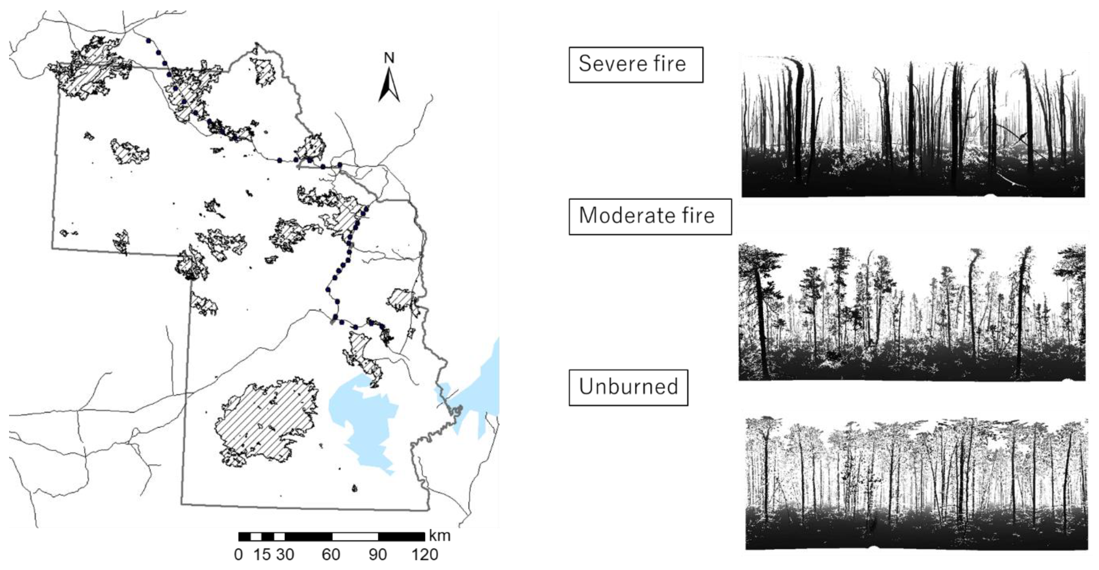
The study site was located at Wood Buffalo National Park (WBNP, Figure 1) in Northwest Territories and Alberta, Canada. WBNP became a national park in 1922 and is a designated wildlife refuge. Lightning is the major source of forest fires [30,31], and the park is located within the area known as the fire hot spot of Canada [32,33]. The dominant tree species are Jack pine (Pinus banksiana Lamb.), aspen (Populus tremuloides Michx.), balsam poplar (Populus balsamifera L.), white spruce (Picea glauca (Moench) Voss), black spruce (Picea Mariana (Mill.) BSP), and tamarack (Larix laricana (Du Roi) K. Koch).
2.2. Methodology
Species composition and stand density are major factors that influence the spectral signature of an area. A change in the spectral reflectance observed by a satellite between either two different sites, or the same site at different times, is likely due to differences in species composition or stand density. The area of our study, i.e., within the boreal forest biome, is covered mainly by homogeneous stands of the same age and species. The spectral signature of the area is thus also mainly homogenous, unless altered by some disturbance event (e.g., fire). The area largely consists of native forest stands that have been self-thinning and undergoing a natural succession process [34,35]. Forest succession entails a relatively simple structural change, and stand development can be related to the spectral change.
The spectral change due to fire is derived from pre- and post-fire Landsat image analysis using the Google Earth Engine platform. The structural components of the forest are measured using a Terrestrial Laser Scanner (TLS) to generate a 3D model of the area. The scans were taken in September of 2016.
To identify the spectral change, both dNBR and RdNBR are calculated. Our area of interest covered 44,807 km2 requiring several Landsat image tiles to cover the extent. We utilize Google Earth Engine (GEE) to visualize and analyze the satellite imagery and use the GEE servers to compute dNBR and RdNBR. The use of an online platform greatly speeds up the processing and spares us the onerous task of downloading and processing gigabytes of image data [36]. To compute dNBR and RdNBR, pre- and post-fire dates need to be identified. However, the fires happened in different times and places within our 44,807 km2 study site. To identify the location and date of each fire, a composite imaging technique is used to make pre- and post-fire images. The composite image technique uses a stack of time-series images to select and store the pixel value when the criteria are matched. In this study, NBR values are stored when NDVI is maximum for pre-fire condition and NBR is minimum for post-fire condition. This process is conducted within the study area using multi-temporal Landsat 8 images with a 16-day revisit cycle during the year of 2016. The images are only selected during the fire season from June 1st to October 1st. Using this date range, we avoid erroneous values caused by snow on the ground in spring and winter. An unburnt area has a high NDVI value while the same area post fire has a low NBR value. The difference between those values is used to produce dNBR and RdNBR values for each pixel.
The dNBR and RdNBR values are compared to structure measurements obtained with TLS. The portable laser sensor TX5 (Trimble Inc., Sunnyvale, CA, USA) is used for data collection. The 3D scan data has the potential to quantify the structural differences more accurately between unburned and recently-burned sites, compared to human visual observation. The position of the scan locations is recorded with a consumer grade GPS unit (Montana 600, Garmin Inc., Olathe, KS, USA) with a location error of 5 m. This locational error is far less than the half pixel size of 30 m Landsat imagery. The TX5 TLS system uses phase shift detection to generate 3D points and the horizontal and vertical scan line resolution is set to 0.0167.
Within our study site, there is a road network bisecting the park in north/south and east/west directions. The TLS locations are chosen along this road network for ease of data collection (Figure 1). A systematic random sampling method is used to select sites to cover the diverse range of tree height and species within the large WBNP area. The scanner collects data every 10 km along the road (black dots along the road in Figure 1). The scanning locations are at least 30 m away from the road (perpendicular to the angle along the road) to insure the scan location is within a Landsat pixel that does not include reflectance from the road. The total 32 TLS scans were collected during Sept. 2016 and covered the diverse structural range from unburned sites to sites with high severity burn (Figure 1). All TLS scanning locations (n = 32) are divided into two groups: unburned plots (no fire since 1981, n = 21) and recently burned plots (most recent fire within the last 3 years, n = 11). Historical fire dates are determined using a fire map provided by the Canadian Park Services.
A multi-step process is used to derive structural metrics from the 3D TLS point clouds (Figure 2). A Digital Terrain Model (DTM) is created from the raw 3D point cloud using the climbing and sliding method [37]. The height of the points is normalized using the derived DTM. Only points within a 15m radius of the scan position are used. A 15 m radius provided a point density sufficient to generate DTMs and is the plot size suggested by the CBI field protocol. The CBI field protocol includes cover change estimation, species identification, dead or live judgement, color change assessment, and soil disturbance estimation. They are not directly comparable to the number of voxels. However, the 3D data can contribute structure measurements by height strata (Box 1). The structure assessment is a major factor to determine CBI values. Therefore, this study is not aimed to compare values between CBI and TLS 3D data. The CBI data needs to be collected twice: right after fire for Initial Assessment (IA) and one year after fire for Extended Assessment (EA). Our field samplings were not collected right after fire. The timing to take our data is different from CBI.
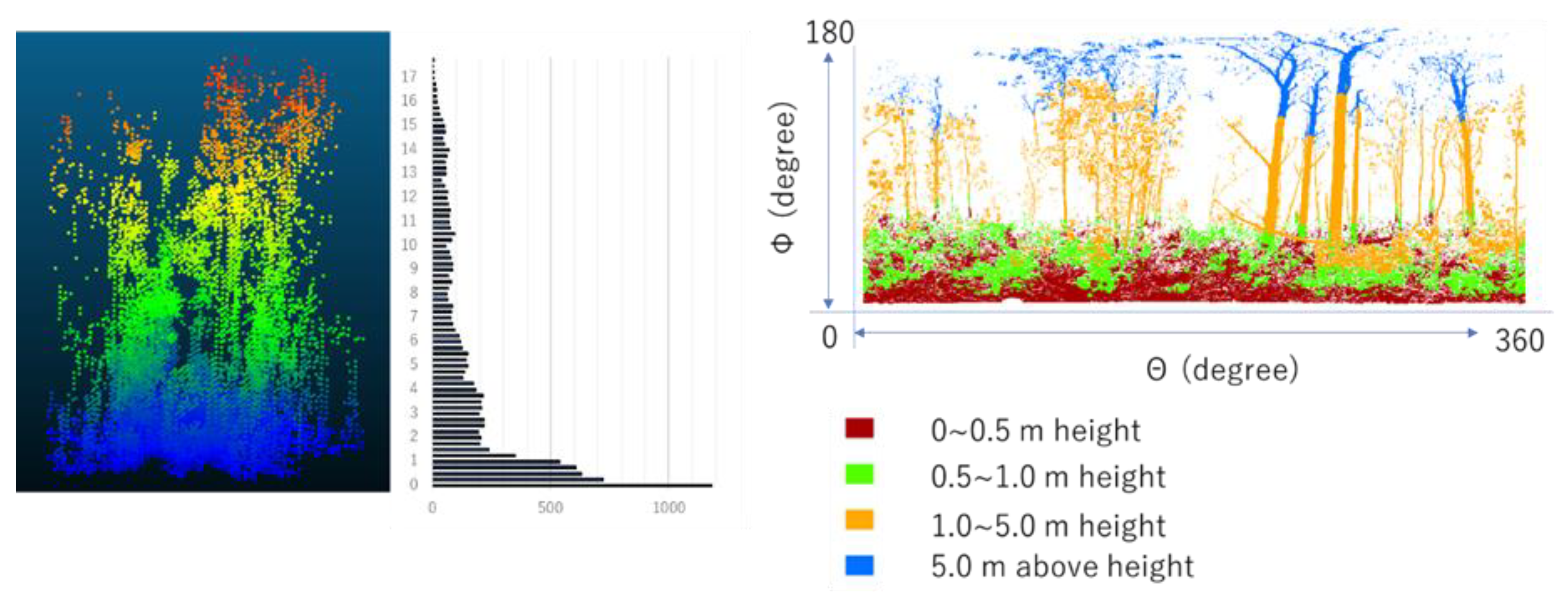
To quantify the vertical forest structure of the scan sites, voxels are created at a 0.25 m resolution. The voxel size is fitted to the average stem diameter of this study site. A voxel is created when there is a laser return point located within a 0.25 m3 grid cell. The number of voxels at different height strata is counted. There are four height strata adapted to this voxel analysis from the original CBI definition: 0 m to 0.5 m (ground surface), 0.5 m to 1m (shrubs), 1 m to 5 m (shrubs and understory), and 5 m above (overstory trees). The number of voxels at each stratum is correlated with the spectral reflectance measured by Landsat. The voxel is used rather than counting the number of raw returns, because the voxel approach can reduce the bias caused by the distance from the sensor and normalizes point density as points are inherently dense and close to the TLS sensor.
The relationship between counted voxels and spectral indices is examined at plot and strata levels. The total voxel count per plot is used to obtain the general relationship. The counts are divided into strata to determine which strata are more significantly related with the spectral change. For the specific strata, the stronger or strongest correlation is found. A linear or non-linear (2nd order polynomial) equation is fitted to the distribution between counted voxels and spectral indices. Both equations used in this study are assessed with R2 values to indicate how strong the correlations are. Moreover, hypothesis tests are applied to test the difference between the linear and non-linear case. The t-test is used for the linear case and Shapiro-Wilk normality test is used for the goodness of fit for the non-linear case. Both cases used a significance level of 0.05. The statistical tests are indicated by p < 0.05 (a significant t-test result) for the linear case and p > 0.05 (a not-significant result with Shapiro-Wilk normality) for the non-linear case.
Box 1. Comparison between Composite Burn Index (CBI) and Terrestrial Lidar Scanning (TLS) measurements.

The CBI is based on visual estimation and judgement to assess vegetation coverage at different height strata (Box 1). To simulate human vision and to derive values based more closely on the CBI protocol, all 3D data are converted to a spherical coordinate system to create a human vision-oriented image (Figure 2 and Figure 3). Based on TLS sensor location, all XYZ 3D coordinates of voxels are converted to three variables in spherical coordinates: distance, horizontal angles (Ɵ), and vertical angles (Φ). The degrees of horizontal and vertical angles are displayed in X and Y axis to make a human vision-oriented image shown in Figure 3. Then, the counted pixels on the image are compared with counted voxels to quantify the visual bias for the different height strata. The voxels displayed in orthogonal coordinates are paired with the satellite image displayed in plain view. To visualize the bias effect, the voxels in each height stratum in the orthogonal coordinates are counted in total, and the number of pixels (in spherical coordinates) visible on the human vision-oriented image in each height strata are also counted. To compare the voxelization method with our simulation of CBI field assessment, the counted total is normalized with the maximum number on a scale from 0 to 1, for each of the height strata, in each scan. A natural logarithmic equation is applied to obtain the non-linear relationship of the visual bias between x in spherical and y in orthogonal coordinates.
3. Results
There were 32 TLS scans in total. Eleven of these were in recently burned plots and 21 in unburned plots. There was a linear relationship between the total number of voxels within each scan in the unburned plots, and satellite derived dNBR (R2 value of 0.54, p value < 0.05) and RdNBR values (R2 value of 0.60, p value < 0.05) (Figure 4). In the burned plots, there was a non-linear correlation with R2 values of 0.75 (p value > 0.05) and 0.73 (p value > 0.05) for dNRR and RdNBR respectively (Figure 4). Similar relationships of dNRR and RdNBR were compared to the number of voxels at each of the four height strata (Figure 5 and Figure 6). There was a negative linear slope for unburned plots and a non-linear relationship for recently burned plots.
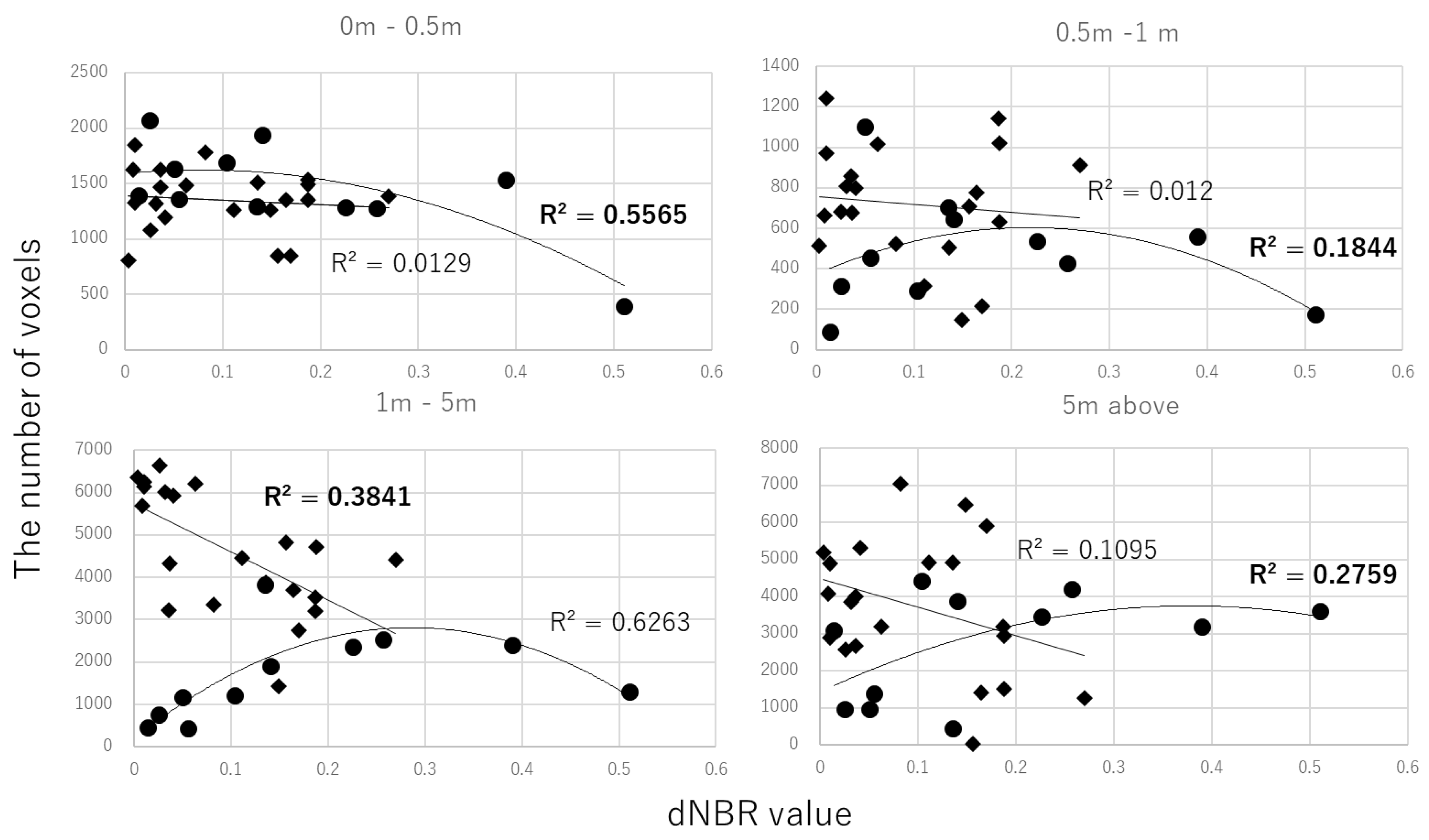
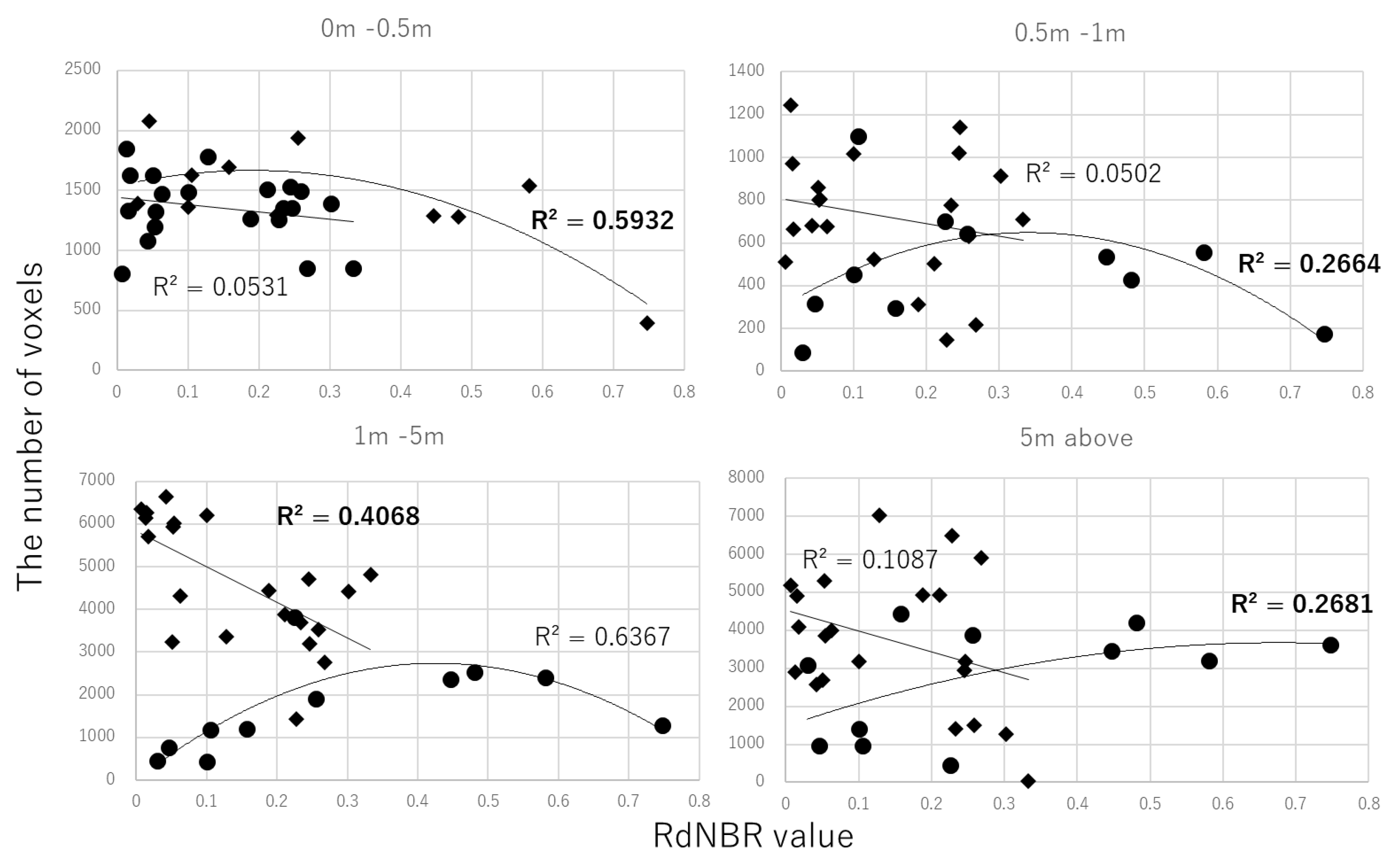
In the recently burned plots, the strongest relationship between voxel counts and dNBR and RdNBR values was in the 0 to 0.5 m height stratum with R2 values of 0.56 for dNBR ( p value > 0.05) and 0.59 for RdNBR ( p value > 0.05). Additionally, for burned plots there were weak correlations in the 0.5 to 1 m and above 5 m height strata with R2 values of 0.18 and 0.28 (p value > 0.05) for dNBR respectively and R2 values of 0.27 and 0.27 (p value > 0.05) for RdNBR respectively. The unburned plots had the strongest relationship between voxel counts and dNBR and RdNBR values in the height stratum between 1 to 5 m, producing R2 values of 0.38 for dNBR (p value < 0.05) and 0.41 for RdNBR (p value < 0.05) in Figure 5 and Figure 6. The results from Figure 5 and Figure 6 found specific height strata only related with the spectral change.
There was a non-linear relationship (visual bias) between the voxel approach and the pixel-based estimation in the three lower strata (0 to 0.5 m, 1 m to 1.5 m, and 1.5 m to 5 m) with a linear relationship in the upper (+5 m) strata (Figure 7). The bias was greatest in the lowest strata.
4. Discussion
Comparing dNBR values with RdNBR and the total number of voxels per plot (Figure 4), the range of RdNBR was wider than the range of dNBR because of the effect of including pre-fire vegetation conditions in the equation. There was no significant difference between R2 values presented in Figure 5 and Figure 6.
For unburned plots, Figure 5 and Figure 6 show that increased numbers of voxels in the height strata (1 to 5 m) were negatively correlated with dNBR and RdNBR, because more vegetation structure developed at the 1 to 5 m height stratum produced less spectral variability in dNBR and RdNBR. The post-fire NBR values approached the pre-fire NBR values due to the structural change at different height strata. For burned-plots, the negative correlation in the lowest (i.e., ground) strata indicated vegetation recovery of the strata. This process of using voxels improves not only the quality of ground observation data but also allows for better correlation with satellite images. Improved illumination values were collected from multi-temporal images through the image compositing process to compute dNBR and RdNBR, and higher precision 3D data were obtained to compare between burned and unburned plots.
The dNBR and RdNBR are relative measurements between pre and post fire NBR. If the site has experienced no fire, they are presumed to be zero. However, there were some changed values at unburned plots in Figure 5 and Figure 6. The slight change was related to the structural difference of the height strata between 1 to 5 m. This shows an advantage to using high precision 3D data to detect small changes in that height stratum. This method is useful to describe ecological response to fire in burned plots and structural development in unburned plots. Through this process, the specific height strata related with the spectral change are identified by the stronger correlations.
For burned plots, the relationship between counted voxels and spectral indices was non-linear (Figure 4, Figure 5 and Figure 6) and was related to the ecological responses of the site conditions. High spectral change (in x axis) with low voxel count (in y axis) characterizes the severely burned sites immediately after fire; middle spectral change with high voxel count means live vegetation remained after fire; and low spectral change with low voxel count means no vegetation recovery after fire.
The bias shown in Figure 7 helps to understand the non-linear relationship [8,14,38,39,40,41] between satellite image analysis such as dNBR and RdNBR and the ground visual assessment of CBI. Previous studies have shown that when simulated CBI was prepared from satellite images there was a linear relationship [42]. However, when the canopy fraction was included in the derived CBI [43], the relationship became non-linear. If the site has vegetation less than 5 m tall, then height strata need to be implemented in the severity measurement; the visual bias produces more deviation from the correlation between satellite and ground observation. The 3D structural data help to visualize the bias in observed vegetation coverage.
The utility of a 2D severity map from spectral indices such as dNBR and RdNBR is limited to assess severity. With 3D ground observations, the spectral change can be addressed by structural change. A good example of this application is fire refugia. The vegetation recovery takes different trajectoris with the initial structure remaining after fire. The severity assessment with 3D ground observation helps to characterize the difference.
Three years were required to detect an ecological response at this study site. The severity is measured by the most immediate fire effects as an immediate assessment and additional responses of initial severity as an extended assessment. The duration of vegetation recovery depends on the ecosystem and the climate of the site. The recovery rate is slow in boreal forest region and the recent fire burned with high intensity. With high intensity fire and slow vegetation recovery, the spectral change observed over burned plots is more related with ecological response. The three year interval was needed to detect the ecological response for fire severity. Monitoring ecological response after fire is an important application of TLS ground observation.
With regard to TLS ground sampling, one third of samples only came from burned plots (Figure 5 and Figure 6). In this study site, the sampling locations were limited to places along the roads due to difficult accessibility. The number of burned plots facing roads were more limited than the number of unburned plots. That is why only one third of samples were from burned plots. The ground sampling strategy can be improved to capture more diverse fire severity.
A TLS limitation for collecting ground forest structure data includes occlusion of laser returns by forest obstacles within the scanning view angle [44,45]. In this study, a sampling approach is applied that isn’t dependent on capturing occlusion free 3D data [16,17]. Our sampling strategy was to compare 3D data among plots by using a single scanning location. Multiple-scans per plot would be better to capture more complete structure measurements as occlusion is eliminated, but multiple scans invite more sampling variation with additional factors of scan positioning and angle being introduced. The single scanning strategy has been adopted to compare different vertical vegetation profiles and describe different structural conditions [46]. Calders and co-authors found that a single scanning was enough to describe various vertical plant profiles. This TLS study does not aim to provide absolute accuracy in tree measurements of the sites, but the results provides more accurate “relative differences” among plots without any subjective judgement, which could not be achieved by conventional visual estimates. This 3D ground truth is needed more in validating fine scale, post fire change when being estimated by high-resolution optical [47] and radar images [48].
5. Conclusions
Forest fire is measured by extent and severity of fire. The objective of this study was to propose a new ground observation technique using 3D data collected by Terrestrial Laser Scanner (TLS) in the field, and to determine its value for ground validation of spectral change on Landsat images. The spectral change between pre- and post-fire is compared with structural differences amongst the sites with different fire severities. To compare them, TLS generated 3D data was changed to voxels, and the number of voxels was counted and compared with dNBR and RdNBR in four different height strata. There was a negative linear relationship in the height strata between 1 m to 5 m for unburned plots and a non-linear relationship in the height strata between 0 to 0.5 m for burned plots. Shrub and understory development was detected in tall shrub strata for unburned plots, and vegetation recovery in the lowest height strata (0 to 0.5 m) was detected for burned-plots. Furthermore, there was a non-linear relationship between visual assessment of CBI and burn indices derived from satellite images. Fine resolution remote sensing imagery is commonly available and accessible through GEE, which will require a more accurate validation method from ground data collection. To make it efficient to collect data and to match the precision of high-resolution data, ground sampling using TLS to derive 3D data will play an important role in improving the correlation between satellite and field data. TLS is especially useful for quick ground assessments which are needed for forest fire applications.
Author Contributions
Conceptualization, A.K. and L.M.M.; methodology, A.K., D.T. and A.T.H.; software, A.K. and D.T.; validation, A.K.; formal analysis, A.K.; writing—original draft preparation, A.K.; writing—review and editing, J.L.B., D.T., L.M.M. and A.T.H.; funding acquisition, A.K.
Funding
This research was supported by the Environment Research and Technology Development Fund of the Ministry of the Environment, Japan, grant number 2RF-1501 and the UW Precision Forestry Cooperative.
Acknowledgments
The authors would like to acknowledge Canadian Park Services for providing the fire map and thank Garrett W. Meigs (Oregon State University, USA) for valuable advice on this research and reviews of this paper, Akira Osawa (Kyoto University) for proving research sites for this study, Yuichi Hayakawa (Hokkaido University, Japan) for proving the TLS sensor for this fieldwork, Mizuki Taga (Olympus Co. Ltd., Japan), and Masuto Ebina (Hokkaido Research Organization, Japan) for their field assistance of TLS data collection for this study.
Conflicts of Interest
The authors declare no conflict of interest.
References
- Hudak, A.T.; Morgan, P.; Bobbitt, M.J.; Smith, A.M.S.; Lewis, S.A.; Letile, L.B.; Robichaud, P.R.; Clark, J.T.; McKinley, R.A. The Relationship of Multispectral Satellite Imagery to Immediate Fire Effects. Fire Ecol. 2007, 3, 64–90. [Google Scholar] [CrossRef]
- Sugihara, N.G.; van Wagtendonk, J.W.; Shaffer, K.E.; Fites-Kaufman, J.; Thode, A.E. Fire in Calfornia’s Ecosystems; University of Calfornia Press: Berkeley and Los Angeles, Calfornia, CA, USA, 2006. [Google Scholar]
- Key, C.H.; Benson, N.C. Landscape assessment (LA): Sampling and analysis methods. FIREMON: Fire Effects Monitoring and Inventory System General Technical Report RMRS-GTR-164-CD. Fort Collins, CO: USDA Forest Service, Rocky Mountain Research Station. 2006. [Google Scholar]
- García López, M.J.; Caselles, V. Mapping Burns and Natural Reforestation using Thematic Mapper Data. Geocarto Intern. 1991, 6, 31–37. [Google Scholar] [CrossRef]
- Koutsias, N.; Karteris, M. Logistic regression modelling of multitemporal Thematic Mapper data for burned area mapping. 1998, 1161. [Google Scholar] [CrossRef]
- Escuin, S.; Navarro, R.; Fernández, P. Fire severity assessment by using NBR (Normalized Burn Ratio) and NDVI (Normalized Difference Vegetation Index) derived from LANDSAT TM/ETM images. Intern. J. Remote Sens. 2008, 29, 1053–1073. [Google Scholar] [CrossRef]
- Miller, J.D.; Thode, A.E. Quantifying burn severity in a heterogeneous landscape with a relative version of the delta Normalized Burn Ratio (dNBR). Remote Sens. Environ. 2007, 109, 66–80. [Google Scholar] [CrossRef]
- Soverel, N.O.; Coops, N.C.; Perrakis, D.D.B.; Daniels, L.D.; Gergel, S.E. The transferability of a dNBR-derived model to predict burn severity across 10 wildland fires in western Canada. Intern. J. Wildland Fire 2011, 20, 518–531. [Google Scholar] [CrossRef]
- Verbyla, D.L.; Kasischke, E.S.; Elizabeth, E.H. Seasonal and topographic effects on estimating fire severity from Landsat TM/ETM + data. Intern. J. Wildland Fire 2008, 17, 527–534. [Google Scholar] [CrossRef]
- Allen, J.L.; Sorbel, B. Assessing the differenced Normalized Burn Ratio’ s ability to map burn severity in the boreal forest and tundra ecosystems of Alaska ’ s national parks. Intern. J. Wildland Fire 2008, 17, 463–475. [Google Scholar]
- Kasischke, E.S.; Turetsky, M.R.; Ottmar, R.D.; French, N.H.F.; Hoy, E.E.; Kane, E.S. Evaluation of the composite burn index for assessing fire severity in Alaskan black spruce forests. Intern. J. Wildland Fire 2008, 17, 515–526. [Google Scholar] [CrossRef]
- Murphy, K.A.; Reynolds, J.H.; Koltun, J.M. Evaluating the ability of the differenced Normalized Burn Ratio ( dNBR ) to predict ecologically significant burn severity in Alaskan boreal forests. Intern. J. Wildland Fire 2008, 17, 490–499. [Google Scholar] [CrossRef]
- Lentile, L.B.; Holden, Z.A.; Smith, A.M.S.; Falkowski, M.J.; Hudak, A.T.; Morgan, P.; Lewis, S.A.; Gessler, P.E.; Benson, N.C. Remote sensing techniques to assess active fire and post fire effects: clarification of terminology. Intern. J. Wildland Fire 2006, 15, 319–345. [Google Scholar] [CrossRef]
- Miller, J.D.; Knapp, E.E.; Key, C.H.; Skinner, C.N.; Isbell, C.J.; Creasy, R.M.; Sherlock, J.W. Calibration and validation of the relative differenced Normalized Burn Ratio (RdNBR) to three measures of fire severity in the Sierra Nevada and Klamath Mountains, California, USA. Remote Sens. Environ. 2009, 113, 645–656. [Google Scholar] [CrossRef]
- Dixon, G.E. Essential FVS: A User’s Guide to the Forest Vegetation Simulator; USDA-Forest Service, Forest Management Service Center: Fort Collins, CO, USA, 2002. [Google Scholar]
- Hackenberg, J.; Spiecker, H.; Calders, K.; Disney, M.; Raumonen, P.; Observation, E.; Group, O.; Road, H.; Street, G.; Liang, X.; et al. SimpleTree—An Efficient Open Source Tool to Build Tree Models from TLS Clouds. Forests 2015, 92, 4245–4294. [Google Scholar] [CrossRef]
- Raumonen, P.; Kaasalainen, M.; Akerblom, M.; Kaasalainen, S.; Kaartinen, H.; Vastaranta, M.; Holopainen, M.; Disney, M.; Lewis, P. Fast Automatic Precision Tree Models from Terrestrial Laser Scanner Data. Remote Sens. 2013, 5, 491–520. [Google Scholar] [CrossRef] [Green Version]
- Seidel, D.; Beyer, F.; Hertel, D.; Fleck, S.; Leuschner, C. 3D-laser scanning: A non-destructive method for studying above- ground biomass and growth of juvenile trees. Agric. For. Meteorol. 2011, 151, 1305–1311. [Google Scholar] [CrossRef]
- Zheng, G.; Moskal, L.M. Computational-Geometry-Based Retrieval of Effective Leaf Area Index Using Terrestrial Laser Scanning. IEEE Trans. Geosci. Remote Sens. 2012, 50, 3958–3969. [Google Scholar] [CrossRef]
- Seidel, D.; Ammer, C.; Puettmann, K. Describing forest canopy gaps efficiently, accurately, and objectively: New prospects through the use of terrestrial laser scanning. Agric. For. Meteorol. 2015, 213, 23–32. [Google Scholar] [CrossRef]
- Paynter, I.; Saenz, E.; Genest, D.; Peri, F.; Erb, A.; Li, Z.; Wiggin, K.; Muir, J.; Raumonen, P.; Schaaf, E.S.; et al. Observing ecosystems with lightweight, rapid-scanning terrestrial lidar scanners. Remote Sens. Ecol. Conserv. 2016. [Google Scholar] [CrossRef]
- Hopkinson, C.; Chasmer, L.; Young-Pow, C.; Treitz, P. Assessing forest metrics with a ground-based scanning lidar. Can. J. For. Res. 2004, 34, 573–583. [Google Scholar] [CrossRef] [Green Version]
- Stovall, A.E.L.; Anderson-Teixeira, K.J.; Shugart, H.H. Assessing terrestrial laser scanning for developing non-destructive biomass allometry. For. Ecol. Manag. 2018, 427, 217–229. [Google Scholar] [CrossRef]
- Lin, Y.; Herold, M. Tree species classification based on explicit tree structure feature parameters derived from static terrestrial laser scanning data. Agric. For. Meteorol. 2016, 216, 105–114. [Google Scholar] [CrossRef]
- Lim, Y.; Hyyppä, J.; Kukko, A.; Jaakkola, A.; Kaartinen, H. Tree Height Growth Measurement with Single-Scan Airborne, Static Terrestrial and Mobile Laser Scanning. Sensors 2012, 12, 12798–12813. [Google Scholar] [CrossRef] [Green Version]
- Calders, K.; Schenkels, T.; Bartholomeus, H.; Armston, J.; Verbesselt, J.; Herold, M. Monitoring spring phenology with high temporal resolution terrestrial LiDAR measurements. Agric. For. Meteorol. 2015, 203, 158–168. [Google Scholar] [CrossRef]
- Metz, J.; Seidel, D.; Schall, P.; Scheffer, D.; Schulze, E.-D.; Ammer, C. Crown modeling by terrestrial laser scanning as an approach to assess the effect of aboveground intra- and interspecific competition on tree growth. For. Ecol. Manag. 2013, 310, 275–288. [Google Scholar] [CrossRef]
- Srinivasan, S.; Popescu, S.C.; Eriksson, M.; Sheridan, R.D.; Ku, N.-W. Multi-temporal terrestrial laser scanning for modeling tree biomass change. For. Ecol. Manag. 2014, 318, 304–317. [Google Scholar] [CrossRef]
- Gupta, V.; Reinke, K.J.; Jones, S.D.; Wallace, L.; Holden, L. Assessing Metrics for Estimating Fire Induced Change in the Forest Understorey Structure Using Terrestrial Laser Scanning. Remote Sens. 2015, 8180–8201. [Google Scholar] [CrossRef]
- Campos-Ruiz, R.; Parisien, M.A.; Flannigan, M.D. Temporal patterns of wildfire activity in areas of contrasting human influence in the Canadian boreal forest. Forests 2018, 9. [Google Scholar] [CrossRef]
- Kochtubajda, B.; Flannigan, M.D.; Gyakum, J.R.; Stewart, R.E.; Logan, K.A.; Nguyen, T.V. Lightning and fires in the Northwest Territories and responses to future climate change. Arctic 2006, 59, 211–221. [Google Scholar] [CrossRef]
- Gillett, N.P.; Weaver, A.J.; Zwiers, F.W.; Flannigan, M.D. Detecting the effect of climate change on Canadian forest fires. Geophys. Res. Lett. 2004, 31. [Google Scholar] [CrossRef] [Green Version]
- Stocks, B.J.; Mason, J.A.; Todd, J.B.; Bosch, E.M.; Wotton, B.M.; Amiro, B.D.; Flannigan, M.D.; Hirsch, K.G.; Logan, K.A.; Martell, D.L.; et al. Large forest fires in Canada, 1959–1997. J. Geophys. Res. 2002, 108. [Google Scholar] [CrossRef]
- Osawa, A. Inverse relationship of crown fractal dimension to self-thinning exponent of treepopulations: a hypothesis. Can. J. For. Res. 1995, 25, 1608–1617. [Google Scholar] [CrossRef]
- Osawa, A.; Kurachi, N. Spatial leaf distribution and self-thinning exponent of Pinus banksiana and Populus tremuloides. Trees 2004, 18, 327–338. [Google Scholar] [CrossRef]
- Gorelick, N.; Hancher, M.; Dixon, M.; Ilyushchenko, S.; Thau, D.; Moore, R. Google Earth Engine: Planetary-scale geospatial analysis for everyone. Remote Sens. Environ. 2017, 202, 18–27. [Google Scholar] [CrossRef]
- Shao, Y.-C.; Chen, L.-C. Automated Searching of Ground Points from Airborne Lidar Data Using a Climbing and Sliding Method. Photogramm. Eng. Remote Sens. 2008, 74, 625–635. [Google Scholar] [CrossRef] [Green Version]
- Hall, R.J.; Freeburn, J.T.; de Groot, W.J.; Pritchard, J.M.; Lynham, T.J.; Landry, R. Remote sensing of burn severity: Experience from western Canada boreal fires. Intern. J. Wildland Fire 2008, 17, 476–489. [Google Scholar] [CrossRef]
- Key, C.H. Ecological and Sampling Constraints on Defining Landscape Fire Severity. Fire Ecol. 2006, 2, 34–59. [Google Scholar] [CrossRef]
- Van Wagtendonk, J.W.; Root, R.R.; Key, C.H. Comparison of AVIRIS and Landsat ETM+ detection capabilities for burn severity. Remote Sens. Environ. 2004, 92, 397–408. [Google Scholar] [CrossRef]
- Zhu, Z.; Key, C.H.; Ohlen, D.; Benson, N. Evaluate Sensitivities of Burn-Severity Mapping Algorithms for Different Ecosystems and Fire Histories in the United States. Final Report to the Joint Fire Science Program. JFSP Project No. 01-1-4-12. Sioux Falls, SD: USGS, National Center for Earth Resources Observation and Science. 2006. [Google Scholar]
- Chuvieco, E.; Riaño, D.; Danson, F.M.; Martin, P. Use of a radiative transfer model to simulate the postfire spectral response to burn severity. J. Geophys. Res. Biogeosci. 2006, 111, 1–15. [Google Scholar] [CrossRef]
- De Santis, A.; Chuvieco, E. GeoCBI: A modified version of the Composite Burn Index for the initial assessment of the short-term burn severity from remotely sensed data. Remote Sens. Environ. 2009, 113, 554–562. [Google Scholar] [CrossRef]
- Zande, D.V.D.; Hoet, W.; Jonckheere, I.; Aardt, J.V.; Coppin, P. Influence of measurement set-up of ground-based LiDAR for derivation of tree structure. Agric. For. Meteorol. 2006, 141, 147–160. [Google Scholar] [CrossRef]
- Zande, D.V.D.; Jonckheere, I.; Stuckens, J.; Verstraeten, W.W.; Coppin, P. Sampling design of ground-based lidar measurements of forest canopy structure and its effect on shadowing. Can. J. Remote Sens. 2009, 34, 526–538. [Google Scholar] [CrossRef]
- Calders, K.; Armston, J.; Newnham, G.; Herold, M.; Goodwin, N. Implications of sensor configuration and topography on vertical plant profiles derived from terrestrial LiDAR. Agric. For. Meteorol. 2014, 194, 104–117. [Google Scholar] [CrossRef]
- Meng, R.; Wu, J.; Schwager, K.L.; Zhao, F.; Dennison, P.E.; Cook, B.D.; Brewster, K.; Green, T.M.; Serbin, S.P. Using high spatial resolution satellite imagery to map forest burn severity across spatial scales in a Pine Barrens ecosystem. Remote Sens. Environ. 2017, 191, 95–109. [Google Scholar] [CrossRef] [Green Version]
- Tanase, M.A.; Kennedy, R.; Aponte, C. Radar Burn Ratio for fire severity estimation at canopy level: An example for temperate forests. Remote Sens. Environ. 2015, 170, 14–31. [Google Scholar] [CrossRef]
Figure 1.
The study site with Terrestrial Lidar Scanning (TLS) locations denoted by ●. The thin black lines are roads and the shaded polygons are recently burned areas (within the last 3 years). To the right, panoramic views of TLS point clouds of different fire conditions.
Figure 1.
The study site with Terrestrial Lidar Scanning (TLS) locations denoted by ●. The thin black lines are roads and the shaded polygons are recently burned areas (within the last 3 years). To the right, panoramic views of TLS point clouds of different fire conditions.

Figure 2.
TLS data analysis procedure.

Figure 3.
Vertical voxel distribution and counting in orthogonal coordinate (left) and human vision-oriented image in spherical coordinates (right).
Figure 3.
Vertical voxel distribution and counting in orthogonal coordinate (left) and human vision-oriented image in spherical coordinates (right).

Figure 4.
The relationship between the total number of voxels at each plot and (a) dNBR and (b) RdNBR values (marker ●: recently burned plots, ♦: unburned plots, the bold fonts of R2 values are statistically significant for the linear case and not-significant for the non-linear case with a significant level of 0.05).

Figure 5.
The relationship between dNBR and the number of voxels at different heights or strata (marker ●: recently burned plot, ♦: unburned plot, the bold fonts of R2 values are statistically significant for the linear case and not-significant for the non-linear case with a significant level of 0.05).

Figure 6.
The relationship between RdNBR and the number of voxels at different heights or strata (marker ●: recently burned plot, ♦: unburned plot, the bold fonts of R2 values are statistically significant for the linear case and not-significant for the non-linear case with a significant level of 0.05).

Figure 7.
The relationship between the number of pixels in spherical coordinates (x) and the number of voxels in orthogonal coordinates (y) by different height strata (both axes are normalized by the maximum number and all R2 values are statistically significant for the linear case and not-significant for the non-linear case with a significant level of 0.05).

© 2019 by the authors. Licensee MDPI, Basel, Switzerland. This article is an open access article distributed under the terms and conditions of the Creative Commons Attribution (CC BY) license (http://creativecommons.org/licenses/by/4.0/).
Share and Cite
MDPI and ACS Style
Kato, A.; Moskal, L.M.; Batchelor, J.L.; Thau, D.; Hudak, A.T. Relationships between Satellite-Based Spectral Burned Ratios and Terrestrial Laser Scanning. Forests 2019, 10, 444. https://0-doi-org.brum.beds.ac.uk/10.3390/f10050444
AMA Style
Kato A, Moskal LM, Batchelor JL, Thau D, Hudak AT. Relationships between Satellite-Based Spectral Burned Ratios and Terrestrial Laser Scanning. Forests. 2019; 10(5):444. https://0-doi-org.brum.beds.ac.uk/10.3390/f10050444
Chicago/Turabian StyleKato, Akira, L. Monika Moskal, Jonathan L. Batchelor, David Thau, and Andrew T. Hudak. 2019. "Relationships between Satellite-Based Spectral Burned Ratios and Terrestrial Laser Scanning" Forests 10, no. 5: 444. https://0-doi-org.brum.beds.ac.uk/10.3390/f10050444
Note that from the first issue of 2016, this journal uses article numbers instead of page numbers. See further details here.