Vertical Distribution of Leaf Area of European Larch (Larix decidua Mill.) and Norway Spruce (Picea abies (L.) Karst.) in Pure and Mixed Stands

Abstract

The growth effects of mixtures are generally assumed to be a result of canopy structure and crown plasticity. Thus, the distribution of leaf area at tree and stand level helps to explain these mixing effects. Therefore, we investigated the leaf area distribution in 12 stands with a continuum of proportions of European larch (Larix decidua Mill.) and Norway spruce (Picea abies (L.) Karst.). The stands were between 40 and 170 years old and located in the northern part of the Eastern Intermediate Alps in Austria at elevations between 900 and 1300 m asl A total of 200 sample trees were felled and the leaf area distribution within their crowns was evaluated. Fitting beta distributions to the individual empirical leaf area distributions, the parameters of the beta distributions were shown to depend on the leaf area of the individual trees and, for spruce, on the proportion of spruce in the stands. With the equations determined, the leaf area distribution of all trees in the stand, and thus its distribution in the stands, was calculated by species and in 2 m height classes. For the individual trees, we found that the leaf area distribution of larch is more symmetric, and its peak is located higher in the crown than it is the case for spruce. Furthermore, the leaf area distribution of both species becomes more peaked and skewed when the leaf area of the trees increases. The mixture only influences the leaf area distribution of spruce in such a way that the higher the spruce proportion of the stand, the higher the leaf area is located within the crown. At the stand level, a strong relationship was found between the proportion of spruce and the distance between the peaks of the leaf area distributions of larch and spruce.

1. Introduction

There is widespread and general agreement that the growth effect of mixtures is a result of canopy structure and crown plasticity of the species involved [1,2,3,4]. Crown length, diameter, cross-sectional area, crown surface area and crown volume lend themselves to the description of canopy packing as a measure of canopy structure and individual tree crown plasticity, i.e., the ability of species to change their crown shape in a way that the species may place their crowns in different niches of the canopy [5,6,7,8].

Because of the eminent role of leaf area in the absorption of light and thus in photosynthesis, mechanistic individual tree growth models use leaf area rather than other crown parameters (e.g., [9,10]). However, leaf area is frequently modelled as an allometric function of the diameter at breast height (dbh) and the stand age (e.g., [11]) or derived from conventional crown measures as crown length (e.g., [12,13]) or crown surface area [14,15]. Leaf area density, i.e., leaf area per crown volume or crown surface area was found to vary considerably [16] and conventional crown measures such as crown length, crown width etc., were shown to insufficiently describe leaf area distribution [17]. Thus, they may only be first approximations for describing the plasticity of leaf area as it may depend on and constitute the canopy structure, which is required in order to understand the mixing effects [18]. This is why the distribution of leaf area within the crowns and within the stands may give better insights into the effects of crown plasticity on mixing effects of growth than only conventional crown characteristics.

There is a considerable amount of mixed stands of European larch (Larix decidua Mill.) and Norway spruce (Picea abies (L.) Karst.) in Central Europe. This mixture of the deciduous conifer and extremely shade-intolerant larch and the much more shade-tolerant spruce has rarely been investigated. The few investigations that have been carried out [3,19] seem to indicate that stand structure plays an important role in the mixing effects on growth.

Therefore, we wanted to:

• investigate the leaf area distribution within the crowns of individual trees of both the involved species,
• study its plasticity with respect to the interspecific environment, and
• compare the vertical leaf area distribution of stands with different species proportions.

2. Materials and Methods

2.1. Location and Study Design

The investigation was conducted in the Alpine biogeographic region in the northern part of the Eastern Intermediate Alps in Austria at approximately 47°26′ east and 15°05′ north. The mean annual temperature and mean annual precipitation are 5.2 °C and 1510 mm, respectively. The prevailing silvicultural management is strip clear cutting [20,21,22], where after felling, the forest is regenerated naturally in three strips. In the inner strip, Norway spruce dominates, while in the outer strip the light-demanding European larch prevails. In the transitional zone, mixed stands of these two species develop (Figure 1). The total strip width is approximately two to three times the height of the dominant trees.

At four locations, we established three plots: one of each forest type (inner, outer, and transitional strip). All plots were on steep Northwest-oriented slopes at altitudes between 900 and 1300 m asl The plot size was between 150 and 1600 m² and was chosen in such a way that each plot contained at least 100 trees of the dominant species. The selected stands can be regarded as nearly even-aged. The mean coefficient of variation of the tree age within the plots, estimated from the sample trees, was about ±5% for spruce and ±10% for larch. The age of the stands varied between 40 and 170 years, the dominant height ranged between 20 and 40 m, the basal area between 30 and 50 m² ha⁻¹, and the stocking degree between 0.7 and 1.0. For the plot characteristics, see

Table 1. Plot characteristics; hdom is the dominant height sensu Assmann [24], MAI is the mean annual increment at age 100 estimated from Marschall [25], dg is the quadratic mean diameter, Stocking is the relative stocking calculated from the relative stand density indices with maxima taken from Vospernik and Sterba [26], Prop. Spruce is the proportion of spruce based on the relative stand density index (SDI), using the maximum density lines as evaluated by Vospernik and Sterba [26] for the 95th percentile.

Plot Characteristics	Spruce Dominated			Spruce-Larch			Larch Dominated
	min	mean	max	min	mean	max	min	mean	max
Plot Size [m2]	2503	6593	16,172	2664	7663	12,886	1379	7708	11,543
Age Spruce [a]	40	95	124	42	117	175	-	-	-
Age Larch [a]	-	-	-	45	114	183	47	109	150
hdom Spruce [m]	18.7	29.4	39.7	19.0	28.7	33.9	-	-	-
hdom Larch [m]	-	-	-	21.5	30.4	34.8	21.2	31.1	39.3
MAI Spruce [m³ a−1 ha−1]	5.9	9.9	15.3	6.1	8.3	9.7	-	-	-
MAI Larch [m³ a−1 ha−1]	-	-	-	6.7	8.3	10.0	8.7	8.9	9.6
dg Spruce [cm]	21.2	35.3	47.2	15.2	32.7	40.5	-	-	-
dg Larch [cm]	-	-	-	27.3	39.1	48.3	22.8	33.8	46.0
Stocking	0.682	0.764	0.868	0.634	0.767	0.977	0.680	0.800	1.010
Prop. Spruce	0.612	0.782	0.929	0.391	0.416	0.464	0.017	0.202	0.392

, for further details please refer to Dirnberger et al. [15] and Sterba et al. [23].

2.2. Data Assessment in the Field

The data that were assessed for all of the trees in the plots were the diameter at breast height (measured by diameter tape at 1.3 m above the forest floor on the uphill side of the tree), the tree height and the height to the crown base (measured by Vertex IV ultrasonic hypsometer [27]), and the tree positions (x- and y-coordinates) within the plot and plumbings to six to eight points of the crown borders (assessed by laser measuring equipment, FieldMap [28]). For the individual tree characteristics, see

Table 2. Individual tree characteristics; dbh is the diameter at breast height, height is the total tree height, hcb is the height of the crown base above the ground, cl is the crown length, cw is the width of the horizontal crown projection, LA is the leaf area, sd is the standard deviation.

Tree Characteristics		All Trees		Sample Trees
		Spruce (n = 2549)	Larch (n = 1422)	Spruce (n = 74)	Larch (n = 120)
dbh [cm]	min	5.0	6.7	9.2	10.3
	mean	30.1	36.1	33.5	36.5
	sd	14.8	11.1	12.7	11.9
	max	81.2	80.2	64.2	62.0
height [m]	min	2.4	6.5	8.1	10.4
	mean	22.6	29.7	25.6	28.9
	sd	9.8	6.4	7.9	7.0
	max	49.4	45.1	39.3	42.8
hcb [m]	min	0.2	1.5	1.0	2.9
	mean	9.4	16.7	10.1	16
	sd	6.1	5.0	5.5	5.7
	max	27.8	31.6	19.2	25.8
cl [m]	min	0.3	1.2	5.0	5.3
	mean	13.2	13	15.5	12.9
	sd	5.8	4.8	4.5	4.1
	max	40.0	42.4	26.1	27.7
cw [m]	min	0.8	1.6	2.3	2.2
	mean	4.7	6.3	4.8	5.6
	sd	1.6	1.9	1.2	2.0
	max	10.7	14.3	8.2	10.7
LA [m2]	min	3.0	5.2	8.3	10.5
	mean	156.8	118.9	172.8	119.3
	sd	135.5	68.0	120.2	86.9
	max	849.9	456.3	613.8	617.2

.

2.3. Sample Trees

In the mixed plots, 15 larch trees and 10 spruce trees and, in the monospecific plots, the same numbers of sample trees of the respective species were selected. Owing to the fact that in three stands only eight8 spruces could be felled, the total sample size yielded 194 trees. While the sample trees were still standing, a total of 24 sample branches per sample tree, eight in each third of the crown length, were lowered on a rope for further processing. Before bringing them down, their diameter at a distance of 2 cm from their insertion at the bole was recorded and its position marked. Then, the trees were felled, and the diameters and the distances from the crown base to the nearest meter of all living branches were recorded. These branches were used to determine their one-sided projected leaf area. For further details, please refer to Dirnberger et al. [15]. For the characteristics of the sample trees, see Table 2.

2.4. Leaf Area and Competition

For each individual single tree, the 24 sample branches were used to estimate the coefficients $a$ and $b$ of an equation $LA=a·d^b$ with $LA$, the leaf area of the branch and $d$ the branch diameter. This equation was then used to estimate the leaf area of all branches of the respective sample tree. These leaf areas had been used by Dirnberger et al. [15] to develop an equation for estimating the whole leaf area of each tree in the stand, as it depended on the crown surface area, the diameter at breast height (dbh) and the stand’s stocking degree for spruce, and on crown surface area, the dbh and the proportion of spruce for larch. With these equations, the total leaf area of all trees in the stands was calculated. For quantifying the fraction of the stand area that was potentially available (APA) for a tree, we used the rasterizing approach [29], based on the circlebow model by Römisch [30]. Thus, the whole plot was rasterized (pixel size = 10 cm × 10 cm) and the squared distance of every pixel to all trees, weighted by their leaf area was calculated (Equation (1)).

$$T_{ij}=\frac{Dis{t}_{ij}^2}{L{A}_j},$$

(1)

with $Dis{t}_{ij}$ the distance from the $i$-th pixel to the $j$-th tree, and $L{A}_j$, the leaf area of the $j$-th tree. The pixel was then assigned to the tree $j$, where $T_{ij}$ is minimal. Thus, a weighted Voronoi diagram of the stand was constructed, resulting in the areas potentially available ($APAs$) of the trees (Figure 2). The leaf area per potentially available area yields the area exploitation index (AEI) according to Gspaltl et al. [29] (Equation (2)).

$$AEI=\frac{LA}{APA},$$

(2)

AEI can be understood as an individual tree density measure characterizing the small-scale competition.

The total boundary $B_{total}$ of the $APA$ of a single tree can be separated into (i) the boundary to spruce neighbours $B_{sp}$ and (ii) the boundary to other species. The proportion of $B_{Sp}$ to $B_{total}$ can then be understood as the contribution of spruce to the overall competition on the respective tree $C_{Sp}$ (Figure 2, Equation (3)).

$$C_{Sp}=\frac{B_{Sp}}{B_{total}}.$$

(3)

For our stands, containing exactly two species, the contribution of larch to the overall competition of a tree $C_{La}$ can also be expressed in terms of $C_{Sp}$ ($C_{La}=1-C_{Sp}$), so that we decided only to use the latter one for further analysis.

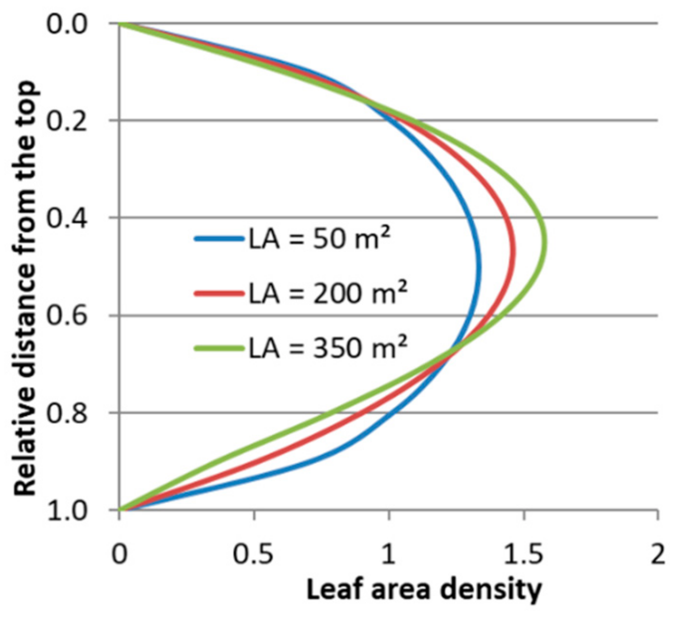
2.5. Leaf Area Distribution

For every sample tree, we fitted a beta distribution to the data of the relative cumulative leaf area as a function of the relative distance $x$ from the top of the tree. Relative means, that the distance is divided by the crown length and thus $x$ is 0 at the top of the tree and 1 at the crown base. The corresponding probability density function is given in Equation (4),

$$f\left(x;p,q\right)=\frac{\Gamma \left(p+q\right)}{\Gamma \left(p\right)\Gamma \left(q\right)}{x}^{p-1}{\left(1-x\right)}^{q-1},$$

(4)

$\Gamma$ is the the gamma function. Following the discussion of Fielitz and Myers [31,32] and Romesburg [33] we decided to estimate the coefficients $p$ and $q$ of the beta distribution by the leaf area weighted relative mean distance of the branch from the top ${\mu }_{dist}$, and the corresponding variance ${\sigma }_{dist}^2$, using Equations (5) and (6) for every tree, rather than using a maximum likelihood approach. Given that the measured distances and leaf areas are no sample, but all branches of a sample tree were observed, deviations between estimates and true parameters may originate from the fact that the beta distribution itself is only an approximation of the discrete empirical leaf area distribution in the crown, rather than from the method of estimation.

$$p=\left(\frac{1-{\mu }_{dist}}{{\sigma }_{dist}^2}-\frac{1}{\mu }\right)·{\mu }^2$$

(5)

$$q=\frac{p}{\mu }-p.$$

(6)

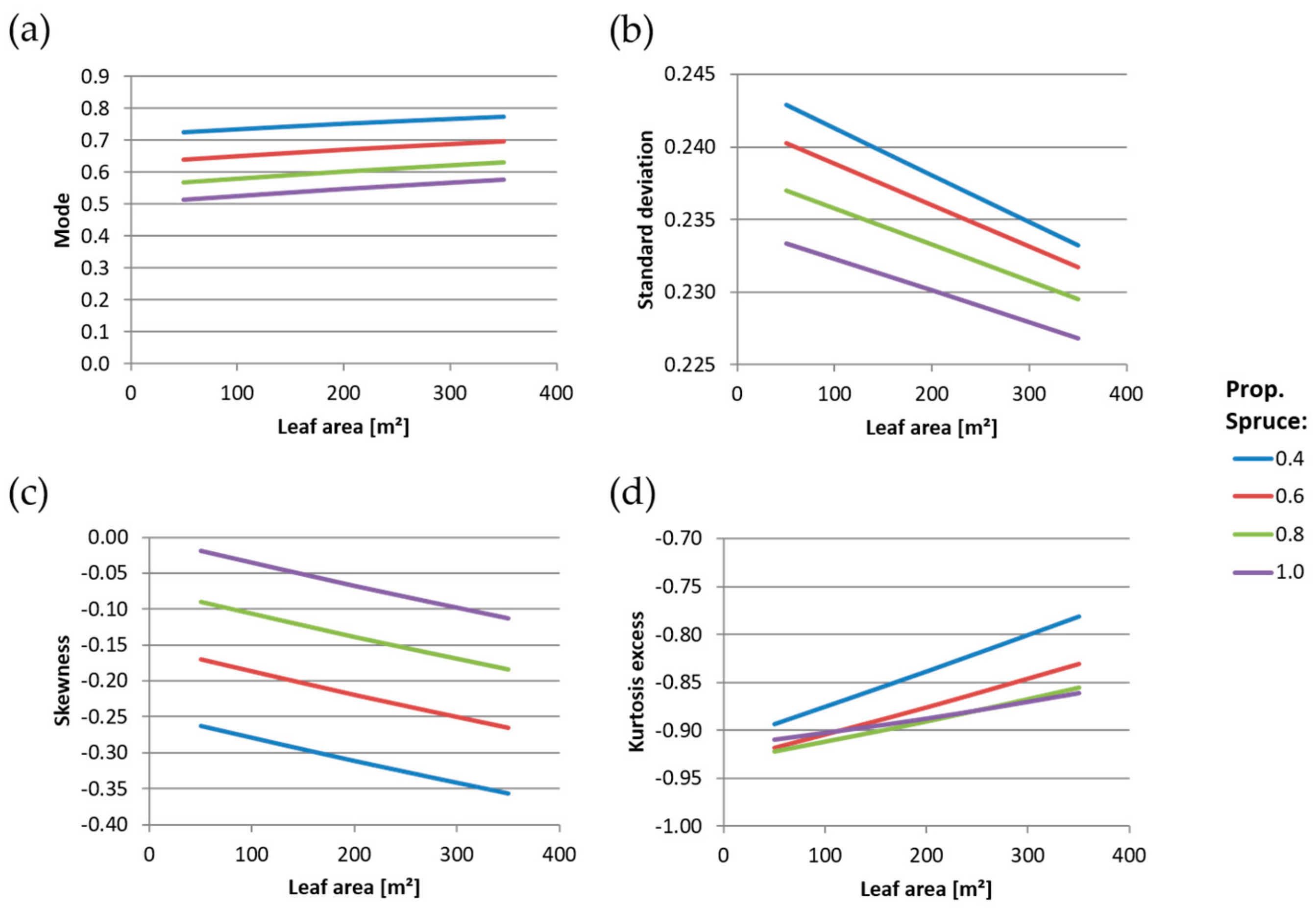
For further characterizing the distribution, the mode, the standard deviation, the skewness and the kurtosis excess were calculated from the parameters $p$ and $q$.

The mode is defined as a value of $x$ were the probability density function (Equation (4)) has its maximum. For our data that means the mode is the relative distance from the top of the tree to the height with the highest density within the crown.

$$\mathrm{Mode}=\frac{p-1}{p+q-2}.$$

(7)

The standard deviation results as:

$$\mathrm{StandardDeviation}=\sqrt{\frac{p·q}{\left(p+q+1\right)·{\left(p+q\right)}^2}}.$$

(8)

The skewness is a measure of the asymmetry of the probability distribution function (pdf), a negative skewness indicates that the tail is on the left side of the pdf, while a positive skewness indicates that the tail is on the right. For our data that means a negative skewness indicates that the leaf area is predominantly located in the lower part of the crown, while a positive skewness indicates that the leaf area is predominantly located in the upper part of the crown.

$$\mathrm{Skewness}=\frac{2\left(q-p\right)}{p+q+2}·\sqrt{\frac{p+q+1}{p·q}}.$$

(9)

The kurtosis excess is defined as kurtosis minus 3, so that an kurtosis excess of zero represents a mesokurtic distribution, while positive and negative kurtosis excess values stand for leptokurtic and platykurtic distributions respectively.

$$\mathrm{KurtosisExcess}=6·\frac{{\left(p-q\right)}^2·\left(p+q+1\right)-p·q·\left(p+q+2\right)}{p·q·\left(p+q+2\right)·\left(p+q+3\right)}.$$

(10)

Then, an investigation into the dependency of the parameters $p$ and $q$ on the sample trees’ traits and their environment was conducted. Therefore, mixed models with individual tree measures and stand measures as fixed effects, and the plot as random effect, were evaluated using the R [34] packages, lme4 [35] and lmerTest [36] the initial model is given by Equation (11).

$$y_{ij}={\beta }_1{x}_{1ij}+\dots +{\beta }_7{x}_{7ij}+{\beta }_8{x}_{8i•}+\cdots +{\beta }_{12}{x}_{12i•}+b_i{z}_{ij}+{ϵ}_{ij}$$

(11)

$y_{ij}$ is the value of the response variable (one of the two parameters $p$ and $q$) for the $j$-th tree at sample plot $i$, ${\beta }_1,\dots ,{\beta }_{12}$ are the fixed-effect coefficients, $b_i$ is the random effect coefficient for sample plot $i$, and ${ϵ}_{ij}$ is the error for tree $j$ at sample plot $i$. The fixed-effect regressors are $x_{1ij},\dots ,x_{7ij}$ for the tree measures, and $x_{8i•},\dots ,x_{12i•}$ for the stand characteristics, $z_{ij}$ is the random-effect regressor. The tree measures were the dbh, the tree height, crown length, crown width, leaf area, local density and the proportion of spruce in the competition. The local density was described by the AEI (Equation (2)) and the proportion of spruce in the competition $C_{Sp}$ (calculated as described by Equation (3) and Figure 2). The stand characteristics were age, quadratic mean diameter, dominant height, stocking and the proportion of spruce. The latter were based on the relative stand density index (SDI), using the maximum density lines as evaluated by Vospernik and Sterba [26] for the 95th percentile. Starting with the full initial model as defined in Equation (11), we used a backward variable selection to reduce model complexity and avoid overfitting.

For each tree in the stand, we then calculated its total leaf area using the equations of Dirnberger et al. [15]. The equations finally determined for the relative leaf area distribution were then used for calculating the leaf area of each tree in two-meter sections, starting at the ground. Thus, we achieved the distribution of leaf area by species in two-meter sections for each plot. The difference between the modes of the stand’s leaf area distribution of larch and that of spruce was then investigated for its relationship with other stands’ characteristics, including spatial distribution characteristics, i.e., species intermingling and horizontal distribution. Species intermingling was described by Pielou’s segregation index [37], based on the nearest neighbor principal. The index is bound between −1 and 1, positive values indicate that the species are segregated, while negative ones indicate association of the different species. An index value of zero means that the probability for a neighboring species is stochastically independent of the species of the subject tree.

The horizontal distribution was characterized by the Clark–Evans index [38], indicating a clustered distribution with values <1 and more regular distributions with values >1. Thus, a CE_spruce < 1 would indicate a stronger horizontal separation of the species and vice versa.

For a detailed description of the indices, see Del Rio et al. [39].

3. Results

3.1. Structural Stand Characteristics

Pielou’s segregation index varies between −0.160 and 0.24 (

Table 3. Leaf area indices and indices characterizing the horizontal spatial distribution of the species. LAI is the leaf area index [m²/m²]; CE is the Clark–Evans index; PIELOU is Pielou’s Segregation index; sd is the standard deviation.

Stand Type	Plot ID	LAI Spruce	LAI Larch	LAI Total	CE Spruce	CE Larch	PIELOU
Spruce	1	8.94	0.16	9.10	1.37	1.22	0.04
	4	8.86	0.20	9.06	1.39	0.95	−0.04
	7	4.69	1.09	5.78	1.05	0.99	0.24
	10	6.55	0.52	7.07	1.21	0.65	0.19
	mean	7.26	0.49	7.75	1.26	0.95	0.11
	sd	2.04	0.43	1.62	0.16	0.23	0.13
Mixed (Spruce+Larch)	2	4.94	2.61	7.55	1.15	1.32	−0.02
	5	4.09	1.26	5.35	1.18	1.08	0.23
	8	4.66	1.58	6.25	1.18	1.20	0.08
	11	3.35	1.61	4.96	1.16	1.05	0.25
	mean	4.26	1.77	6.03	1.17	1.16	0.13
	sd	0.70	0.58	1.15	0.02	0.12	0.13
Larch	3	3.98	3.66	7.64	1.13	1.32	−0.16
	6	1.91	3.50	5.41	1.19	1.26	−0.15
	9	1.86	3.72	5.58	0.98	1.13	0.07
	12	0.15	3.57	3.72	0.87	1.18	0.23
	mean	1.97	3.61	5.59	1.04	1.22	0.00
	sd	1.57	0.10	1.61	0.14	0.08	0.19

), indicating that the spatial species distribution varies between slightly associated and segregated. Clark–Evans index varies between 0.65 and 1.39, indicating that the spatial distribution of both species varies between aggregated (<1) and segregated (>1) (Table 3). There were no significant correlations between the structural characteristics and the stocking. Only Pielou’s segregation index slightly, but significantly increased with age, indicating that the species became more horizontally segregated when the stands grow older. No other indices correlate with the stand age. Interestingly, the Clark–Evans indices of spruce and larch are not correlated (R² = 0.0018).

Furthermore, the stocking (from the relative stand density indices of the species) and the species’ proportions by area may characterize the structure of the stand. The stand age effectively characterizes the stand’s developmental stage.

3.2. Leaf Area Distribution within Individual Trees

For the statistics of the estimated coefficients of the individually fitted beta distributions $p$ and $q$ see

Table 4. Parameter estimates (±standard deviation) for $p$ and $q$ of the beta distribution by species. n is the number of sample trees. Δ is the difference between the species. t, the t-statistic for the test of the difference against zero, and p, the respective type-one error probability. • and *** indicate the significance for type-one error probabilities of 10% and 0.1%, respectively.

Parameter	Spruce (n = 74)	Larch (n = 120)	Δ	t	p
$p$	1.916 (±0.342)	1.777 (±0.562)	0.139	1.915	0.0570 •
$q$	1.450 (±0.323)	1.725 (±0.631)	−0.275	−3.480	0.0006 ***

. The differences between the mean parameters were almost ($p$) and highly ($q$) statistically significant.

The leaf area distributions that result from these means show that, generally, the distribution in larch was rather symmetric, while in spruce it is it was rather left skewed, meaning that the leaf area of spruce is located deeper in the crown. The peak of the leaf area distribution of spruce was located at a relative distance from the top of 0.70 ± 0.18 (standard deviation), which is deeper in the crown than for larch with 0.53 ± 0.21 (Figure 3).

It was to be expected that the distribution even within the species may vary depending on other tree or stand characteristics. As a result from the backward variable selection of the initial model (Equation (11)), we found that the parameter $p$ depends only on the leaf area of the individual tree in both species. The parameter $q$ for larch depends only on the leaf area as well, while for spruce it depends only on the proportion of spruce. Parameter estimates and statistics are given in

Table 5. The coefficients and variances of the model in Equation (11). * and *** indicate the significance for type-one error probabilities of 5% and 0.1%, respectively.

Species		p	$\mathbf{Indep} \mathbf{var} \left(\mathit{x}\right)$	q	$\mathbf{Indep} \mathbf{var} \left(\mathit{x}\right)$
Larch	${\beta }_0$	1.511 ***	Leaf area [m2]	1.544 ***	Leaf area [m2]
	${\beta }_1$	0.0223 ***		0.00143 *
	σ2plot	0.0295		0.1268
	σ2tree	0.2412		0.2574
	R2conditional	0.275		0.395
Spruce	${\beta }_0$	1.777 ***	Leaf area [m2]	0.997 ***	Spruce proportion
	${\beta }_1$	0.000808 *		0.7763 *
	σ2plot	0.04678		0.01369
	σ2tree	0.08525		0.0754
	R2conditional	0.351		0.305

.

The resulting leaf area distributions for larch and spruce can be seen in Figure 4 and Figure 5, respectively.

Interestingly, the spruce proportion by area at the stand level significantly influences the parameter $q$, while the spruce proportion in the competition ($C_{Sp}$) of the immediate neighbors does not.

In larch, the leaf area distribution of trees with small leaf areas was less peaked than in trees with large leaf areas (Figure 4), which was effectively reflected by a positive relationship between the kurtosis excess of the distribution with the leaf area. This seems to contradict Williams et al. [18], who found that “western larch allocates foliage into a more diffuse distribution as the crown lengthens”. In order to determine if our relationship is an artefact from the fitting of the beta distributions, we also investigated the relationship as it is calculated from the original tree data without fitting a beta distribution, and the leaf area and the crown length, respectively (Figure 5).

The results show that the positive relationships between kurtosis excess and leaf area and kurtosis excess and crown length held in both cases, with the kurtosis excess when calculated from the original data, as well as with the kurtosis excess when calculated from the parameters of the fitted beta distribution. Additionally, the relationship of kurtosis excess with leaf area was stronger than kurtosis excess with crown length.

For spruce, the leaf area distribution depends not only on the individual tree leaf area but also on the spruce proportion of the stand (Table 5, Figure 6). In stands with a high spruce proportion, the distribution is almost symmetric, while, with decreasing spruce proportion, its skewness increases and the leaf area is located deeper in the crown. Again, similar to larch, the distribution becomes narrower as the leaf area of the tree increases. This visual impression is confirmed by the relationships between the statistics calculated from the beta distribution and the leaf area and the spruce proportion (Figure 7).

3.3. Leaf Area Distribution on the Stand Level

An exemplary leaf area distribution at the stand level is depicted in Figure 8. Calculating the modes of the respective distributions by species, the difference of the modes ($\Delta$ Mode) can be understood as a measure for the complementarity in tree crowns of the species [18]. The larger this difference, the higher the complementarity of the leaf area, thus using different niches for the species (Figure 8,

Table 6. The variation of the modes by species, and Δ Mode at the stand level. R² for Δ Mode and Stocking is 0.0018 (linear), the one for Δ Mode and Prop. Spruce (potential) is 0.85. *** indicating the significance for type-one error probability of 0.1%, for a one sample t-test against zero.

Plot ID	Stocking	Prop. Spruce	Mode Spruce [m]	Mode Larch [m]	Δ Mode [m]
1	0.812	0.929	10.9	14.1	3.2
2	0.740	0.400	5.7	11.8	6.1
3	1.006	0.392	5.6	14.3	8.6
4	0.693	0.868	26.1	28.5	2.5
5	0.631	0.408	21.1	25.7	4.6
6	0.736	0.207	12.3	24.3	12.0
7	0.869	0.609	18.2	22.3	4.1
8	0.973	0.464	18.7	25.6	6.8
9	0.756	0.193	14.5	28.7	14.3
10	0.680	0.722	14.7	19.2	4.5
11	0.712	0.371	18.0	23.3	5.3
12	0.676	0.017	6.9	23.5	16.5
Mean	0.774	0.465	14.4	21.8	7.4 ***

).

Generally, the mode of the leaf area distribution of spruce lies below the mode of larch; however, the difference still exhibits a large variation.

The difference between the modes of the vertical leaf area distribution varies between 2.5 and 16.5 m, meaning that there are stands with strong leaf area competition (i.e., with poor complementarity), where the leaf areas of the species are not vertically separated (Table 6), and conversely stands with low leaf area competition (i.e., high complementarity), where the leaf areas are strongly vertically separated. Only the species proportion, the Clark–Evans index of spruce and the difference between the leaf area modes of the species are considerably correlated (Figure 9). It is evident that the smaller the spruce proportion in the stand the greater is the difference in the modes of the leaf area distributions of the stand.

4. Discussion

4.1. Leaf Area Distribution in Individual Trees

We found the peak of the leaf area distribution of spruce being located deeper in the crown than for larch. This agrees with Guisasola et al. [4], who found, in Chinese subtropical forests, that the relative depth into the crown of the peak of the leaf area depends on the shade tolerance of the species, in such a way that it was highest in the least shade-tolerant species while it was lowest in the most-shade tolerant species. Our mean values for the peaks are in good agreement with the ranking suggested by Guisasola et al. [4]; between 0.5 for the shade-intolerant Liquidambar formosana and 0.7 for the most shade-tolerant, Canopsis eyrei.

The change in the parameters $p$ and $q$ for larch resulted mainly in a change of the kurtosis excess of the leaf area distribution in such a way that the distribution is more uniform and less peaked when the tree’s leaf area is small, and more peaked with increasing leaf area. This also held for the kurtosis excess when calculated from the original data before fitting the beta distribution; therefore, it cannot be an effect that originates from choosing the beta distribution for fitting. This result is different from Williams et al. [18], who found that with increasing crown length the leaf area distribution became more ”diffuse”. When comparing the data used by Williams et al. [18], the minimum dbh, tree height and crown length and crown foliar mass were about the same; however, the means indicated that our sample included much larger trees with a mean dbh of 36 cm compared with the value of 25 cm reported by Williams et al. [18], a mean tree height of 29 m compared with 20 m and a mean foliar mass of 10 kg compared with about 5 kg. Since the age was not given by Williams et al. [18], we can only guess that our sample included older stands or was grown on better-than-average sites. This is supported by Williams et al. [18], who comment that for their largest trees they found the opposite effect, i.e., for large trees the leaf area distribution became more diffuse with decreasing crown length.

The mixture only influences the leaf area distribution in spruce. Interestingly, it is not the mixing within the immediate neighborhood of the respective tree ($C_{Sp}$) but rather the mixture at the stand’s scale, i.e., the proportion of spruce by area in the plot. The higher the spruce proportion in the stand, the more symmetric, with a peak higher up in the crown, the leaf area distribution of individual spruce trees is. A possible explanation is that more spruce in the stand results in a higher intraspecific competition between the spruce trees. Under high intraspecific competition, light is a limiting factor, therefore the leaf area of the trees shifts upwards if the competition is high. Considering the Δ Mode decreases with increasing spruce proportion, this agrees with Weiskittel et al. [40] who found that for shade-tolerant evergreens, the leaf area shifted upwards in the crown into a more mono-layered distribution. Williams et al. [18] attribute this effect to a balancing act between minimizing water loss while maximizing light capture. Even for the shade-intolerant larch, Fellner et al. [41] found a reflection of both these effects in the specific leaf area, depending on both the canopy depth and the branch height. Mechanical abrasion of branches and leaves has been found to change crown form [42] and thus may also alter the leaf area distribution of individual trees. Hajek et al. [43] even argue that the main canopy interaction in temperate mixed forests is mechanical abrasion and not competition for light. If this holds for larch-spruce mixtures, the effect of the spruce proportion on the leaf area distribution would mean a higher proportion of larch would cause the peak of the leaf area of spruce to move downwards in the crown. This could be attributed to the whip-form twigs of larch. Since we, however, did not find a significant influence of the stand density on the parameters $p$ and $q$ of the beta distribution, an influence of crown abrasion on the leaf area distribution seems doubtful. Our data however, do not support an important role of this effect because none of the parameters p and $q$ has been found to depend significantly on stand density.

4.2. Vertical Leaf Area Distribution at the Stand Scale

At the stand scale we described the complementarity of leaf area as possible causes for mixing effects vertically by the difference between the peaks of the leaf area distributions of the two species ($\Delta$ Mode) and horizontally by the Clark–Evans index, indicating the spatial aggregation of the species.

Large differences between the peaks of the leaf area distribution and horizontally aggregated distribution of the species would indicate that the species use different niches for their leaf area and thus, by mitigating interspecific competition let expect positive mixing effects on growth [8]. Probably the relationship of the $\Delta$ Mode as well as the proportion of spruce is steered by the development of the stands. However, it was not the intention to describe and discuss the silvicultural development of the strip clear cut system but rather to investigate if there are mixing effects on the leaf area distributions of spruce and larch at the individual tree and at the stand level. The design of the study was therefore to have mixed and pure stands at all ages. Therefore, it is surprising, that there is no correlation between the proportion of spruce and the age. The main question however, if there is a mixing effect on the leaf area distribution at the stand level, is positively answered by the high correlation between the proportion of spruce and the differences of the peaks of the leaf area distributions of larch and spruce. The same is true for the lower, but also significant correlation between the Clark–Evans index and the $\Delta$ Mode. The species obviously react with their leaf area distributions in a way that they use different niches in space.

5. Conclusions

At the individual tree scale, we conclude that the leaf area distribution of larch is more symmetric and its peak is higher up in the crown than in spruce, which can be attributed to the difference in shade tolerance of these two species. With increasing leaf area of the trees, the leaf area distribution of both species becomes more peaked and skewed. The mixture influences the leaf area distribution of spruce in such a way that the higher the spruce proportion of the stand, the higher up in the crown its leaf area is located, i.e., the more mono-layered it is. This effect may be attributed to a balancing act between minimizing water loss while maximizing light capture [18].

At the stand scale, there is a clear mixing effect on the leaf area distribution. Structural characteristics, such as vertical distance between peaks of the leaf area distributions of the species and the increasing horizontal aggregation of spruce are clearly correlated with the proportion of spruce. The nearer the stand approaches a pure spruce stand, and the more uniform the horizontal distribution of spruce is, the less separated the leaf areas of the species are. Conversely with increasing the mixture, the complementarity of the leaf area distribution increases too. Niche partitioning and interspecific competition for light seem not to be the most important drivers for mixing effects in these mixtures, and further research is needed to identify these crucial drivers.

References

1. Jucker, T.; Bouriaud, O.; Coomes, D.A. Crown plasticity enables trees to optimize canopy packing in mixed-species forests. Funct. Ecol. 2015, 29, 1078–1086. [Google Scholar] [CrossRef]
2. Dieler, J.; Pretzsch, H. Morphological plasticity of European beech (Fagus sylvatica L.) in pure and mixed-species stands. For. Ecol. Manag. 2013, 295, 97–108. [Google Scholar] [CrossRef]
3. Forrester, D.I.; Ammer, C.; Annighöfer, P.J.; Barbeito, I.; Bielak, K.; Bravo-Oviedo, A.; Coll, L.; del Río, M.; Drössler, L.; Heym, M.; et al. Effects of crown architecture and stand structure on light absorption in mixed and monospecific Fagus sylvatica and Pinus sylvestris forests along a productivity and climate gradient through Europe. J. Ecol. 2018, 106, 746–760. [Google Scholar] [CrossRef]
4. Guisasola, R.; Tang, X.; Bauhus, J.; Forrester, D.I. Intra- and inter-specific differences in crown architecture in Chinese subtropical mixed-species forests. For. Ecol. Manag. 2015, 353, 164–172. [Google Scholar] [CrossRef]
5. Pretzsch, H.; Schütze, C. Crown allometry and growing space efficiency of Norway spruce (Picea abies [L.] Karst.) and European beech (Fagus sylvatica L.) in pure and mixed stands. Plant Biol. 2005, 7, 628–639. [Google Scholar] [CrossRef] [PubMed]
6. Purves, D.W.; Lichstein, J.W.; Pacala, S.W. Crown plasticity and competition for canopy space: A new spatially implicit model parameterized for 250 North American tree species. PLoS ONE 2007, 2, e870. [Google Scholar] [CrossRef] [PubMed]
7. Pretzsch, H.; Dieler, J. Evidence of variant intra- and interspecific scaling of tree crown structure and relevance for allometric theory. Oecologia 2012, 169, 637–649. [Google Scholar] [CrossRef] [PubMed] [Green Version]
8. Pretzsch, H. Canopy space filling and tree crown morphology in mixed-species stands compared with monocultures. For. Ecol. Manag. 2014, 327, 251–264. [Google Scholar] [CrossRef] [Green Version]
9. Duursma, R.A.; Medlyn, B.E. MAESPA: A model to study interactions between water limitation, environmental drivers and vegetation function at tree and stand levels, with an example application to [CO2] × drought interactions. Geosci. Model Dev. 2012, 5, 919–940. [Google Scholar] [CrossRef]
10. Waring, R.H.; Landsberg, J.J. A generalised model of forest productivity using simplified concepts of radiation-use efficiency, carbon balance and partitioning. For. Ecol. Manag. 1997, 95, 209–228. [Google Scholar]
11. Forrester, D.I.; Benneter, A.; Bouriaud, O.; Bauhus, J. Diversity and competition influence tree allometric relationships—Developing functions for mixed-species forests. J. Ecol. 2017, 105, 761–774. [Google Scholar] [CrossRef]
12. Socha, J.; Wezyk, P. Allometric equations for estimating the foliage biomass of Scots pine. Eur. J. For. Res. 2007, 126, 263–270. [Google Scholar] [CrossRef]
13. Eckmüllner, O. Allometric relations to estimate needle and branch mass of Norway spruce and Scots pine in Austria. Austrian J. For. Sci. 2006, 123, 7–15. [Google Scholar]
14. Gspaltl, M.; Sterba, H. An approach to generalized non-destructive leaf area allometry for Norway spruce and European beech Zerstörungsfreie Blattflächen Allometrie für Fichte und Buche Kurzbeschreibung. Austrian J. For. Sci. 2011, 128, 219–250. [Google Scholar]
15. Dirnberger, G.; Kumer, A.-E.; Schnur, E.; Sterba, H. Is leaf area of Norway spruce (Picea abies L. Karst.) and European larch (Larix decidua Mill.) affected by mixture proportion and stand density? Ann. For. Sci. 2017, 74, 8. [Google Scholar] [CrossRef]
16. Seidel, D.; Fleck, S.; Leuschner, C.; Hammett, T. Review of ground-based methods to measure the distribution of biomass in forest canopies. Ann. For. Sci. 2011, 68, 225–244. [Google Scholar] [CrossRef] [Green Version]
17. Martin-Ducup, O.; Schneider, R.; Fournier, R.A. Analyzing the vertical distribution of crown material in mixed stand composed of two temperate tree species. Forests 2018, 9, 673. [Google Scholar] [CrossRef]
18. Williams, G.M.; Nelson, A.S.; Affleck, D.L.R. Vertical distribution of foliar biomass in western larch (Larix occidentalis). Can. J. For. Res. 2017, 48, 42–57. [Google Scholar] [CrossRef]
19. Zöhrer, F. Bestandeszuwachs und Leistungsvergleich montan-subalpiner Lärchen-Fichten-Mischbestände. Forstwissenschaftliches Cent. 1969, 88, 41–63. [Google Scholar] [CrossRef]
20. Allison, T.D.; Art, H.W.; Cunningham, F.E.; Teed, R. Forty-two years of succession following strip clearcutting in a northern hardwoods forest in northwestern Massachusetts. For. Ecol. Manag. 2003, 182, 285–301. [Google Scholar] [CrossRef]
21. Heitzman, E.; Pregitzer, K.S.; Miller, R.O.; Lanasa, M.; Zuidema, M. Establishment and development of northern white-cedar following strip clearcutting. For. Ecol. Manag. 1999, 123, 97–104. [Google Scholar] [CrossRef]
22. Rondon, X.J.; Gorchov, D.L.; Elliott, S.R. Assessment of economic sustainability of the strip clear-cutting system in the Peruvian Amazon. For. Policy Econ. 2010, 12, 340–348. [Google Scholar] [CrossRef]
23. Sterba, H.; Dirnberger, G.; Ritter, T. The Contribution of Forest Structure to Complementarity in Mixed Stands of Norway Spruce (Picea abies L. Karst) and European Larch (Larix decidua Mill.). Forests 2018, 9, 410. [Google Scholar] [CrossRef]
24. Assmann, E. The Principles of Forest Yield Study: Studies in the Organic Production, Structure, Increment, and Yield of Forest Stands; Pergamon Press: Oxford, UK, 1970; ISBN 9780080066585. [Google Scholar]
25. Marschall, J. Hilfstafeln für die Forsteinrichtung; Agrarverlag: Wien, Austria, 1992; ISBN 978-3-7040-1147-3. [Google Scholar]
26. Vospernik, S.; Sterba, H. Do competition-density rule and self-thinning rule agree? Ann. For. Sci. 2015, 72, 379–390. [Google Scholar] [CrossRef]
27. Haglöf Measurement Solutions in Forest and Field. Available online: http://www.haglofcg.com/index.php/en/products/instruments/height/341-vertex-iv (accessed on 9 April 2019).
28. IFER Field-Map—Tool Designed for Computer Aided Field Data Collection. Available online: http://www.fieldmap.cz/ (accessed on 9 April 2019).
29. Gspaltl, M.; Sterba, H.; O’Hara, K.L. The relationship between available area efficiency and area exploitation index in an even-Aged coast redwood (Sequoia sempervirens) stand. Forestry 2012, 85, 567–577. [Google Scholar] [CrossRef]
30. Römisch, K. Durchmesserwachstum und ebene Bestandesstruktur am Beispiel der Kiefernversuchsfläche Markersbach. In DVFFA-Sektion Forstliche Biometrie und Informatik; Hempel, G., Ed.; Deutscher Verband Forstlicher Forschungsanstalten: Tharandt, Germany, 1995; pp. 84–101. [Google Scholar]
31. Fielitz, B.D.; Myers, B.L. Estimation of parameters in the beta distribution. Decis. Sci. 1975, 6, 1–13. [Google Scholar] [CrossRef]
32. Fielitz, B.D.; Myers, B.L. Estimation of parameters in the beta distribution—Reply. Decis. Sci. 1976, 7, 163–164. [Google Scholar]
33. Romesburg, H.C. Estimation of Parameters in the Beta Distribution: Comment. Decis. Sci. 1976, 7, 162. [Google Scholar] [CrossRef]
34. R Development Core Team. R: A Language and Environment for Statistical Computing; R Foundation for Statistical Computing: Vienna, Austria, 2018. [Google Scholar]
35. Bates, D.; Mächler, M.; Bolker, B.; Walker, S. Fitting Linear Mixed-Effects Models Using {lme4}. J. Stat. Softw. 2015, 67, 1–48. [Google Scholar] [CrossRef]
36. Kuznetsova, A.; Brockhoff, P.B.; Christensen, R.H.B. {lmerTest} Package: Tests in Linear Mixed Effects Models. J. Stat. Softw. 2017, 82, 1–26. [Google Scholar] [CrossRef]
37. Pielou, E.C. Mathematical Ecology; Wiley: Hoboken, NJ, USA, 1977. [Google Scholar]
38. Clark, J.; Evans, F.C. Distance to nearest neighbor as a measure of spatial relationships in populations. Ecology 1954, 35, 445–453. [Google Scholar] [CrossRef]
39. Del Río, M.; Pretzsch, H.; Alberdi, I.; Bielak, K.; Bravo, F.; Brunner, A.; Condés, S.; Ducey, M.J.; Fonseca, T.; von Lüpke, N.; et al. Characterization of the structure, dynamics, and productivity of mixed-species stands: Review and perspectives. Eur. J. For. Res. 2016, 135, 23–49. [Google Scholar] [CrossRef]
40. Weiskittel, A.R.; Kershaw, J.A.; Hofmeyer, P.V.; Seymour, R.S. Species differences in total and vertical distribution of branch- and tree-level leaf area for the five primary conifer species in Maine, USA. For. Ecol. Manag. 2009, 258, 1695–1703. [Google Scholar] [CrossRef]
41. Fellner, H.; Dirnberger, G.F.; Sterba, H. Specific leaf area of European Larch (Larix decidua Mill.). Trees 2016, 30, 1237–1244. [Google Scholar] [CrossRef] [PubMed]
42. Putz, F.E.; Parker, G.G.; Archibald, R.M. Mechanical interactions by abrasion. Am. Midl. Nat. 1984, 112, 24–28. [Google Scholar] [CrossRef]
43. Hajek, P.; Seidel, D.; Leuschner, C. Mechanical abrasion, and not competition for light, is the dominant canopy interaction in a temperate mixed forest. For. Ecol. Manag. 2015, 348, 108–116. [Google Scholar] [CrossRef]
Figure 1. Example of an experimental stand under strip clear cutting management (Photo: Dirnberger).
Forests 10 00570 g001
Figure 2. The spruce contribution to individual tree competition ( C s p ) is the proportion of the boundary of the area potentially available (APA) of the subject tree which is bordered by spruce. (a): A spruce (red) surrounded by seven other spruces and three larches, the proportion of the boundary to spruce (yellow lines) to the total boundary is C s p = 0.748. (b): A larch (blue) surrounded by three other larches and two spruces, the proportion of the boundary to spruce (yellow lines) to the total boundary is C s p = 0.424.
Forests 10 00570 g002
Figure 3. The predicted vertical distribution of the leaf area by species.
Forests 10 00570 g003
Figure 4. The predicted vertical distribution of the leaf area of larch, obtained by a linear mixed effect model (Equation (11)) with parameter estimates from Table 5, depending on the individual tree leaf area (LA).
Forests 10 00570 g004
Figure 5. (a): The relationship between the individual tree leaf area of larch and the kurtosis excess of the leaf area distribution. (b): The relationship between the individual crown length of larch and the kurtosis excess of the leaf area distribution. Regression lines in (a,b) are once calculated from the original data without fitting a beta distribution (original data) and once calculated from the estimated parameters. *** indicates the significance for type-one error probability of 0.1%.
Forests 10 00570 g005
Figure 6. The predicted vertical distribution of the leaf area of spruce, obtained by a linear mixed effect model (Equation (11)) with parameter estimates from Table 5, depending on thespruce proportion of the stand (Prop. Spruce) for different individual tree leaf areas (LA). (a): LA = 50 m2, (b): LA = 200 m2 and (c): LA = 350 m2.
Forests 10 00570 g006
Figure 7. Statistics of the leaf area distribution of spruce, calculated from the parameters p and q as estimated from Equation (11) with coefficients from Table 5. (a): Mode (Equation (7)), (b): Standard deviation (Equation (8)), (c): Skewness (Equation (9)) and (d): Kurtosis excess (Equation (10)).
Forests 10 00570 g007
Figure 8. Leaf area distribution by species and height within an exemplary stand (Plot ID = 9).
Forests 10 00570 g008
Figure 9. (a): The relationship between proportion of spruce and Clark–Evans index. (b): The relationship between Δ Mode of the stands’ leaf area distribution and Clark–Evans index. (c): The relationship between proportion of spruce and Δ Mode of the stands’ leaf area distribution. (ac): ** and *** indicate the significance for type-one error probabilities of 1% and 0.1% respectively. Non-significant (n.s.) regression lines are depicted dashed.
Forests 10 00570 g009