Article

Estimating Forest Aboveground Carbon Storage in Hang-Jia-Hu Using Landsat TM/OLI Data and Random Forest Model

1
State Key Laboratory of Subtropical Silviculture, Zhejiang A & F University, Hangzhou 311300, China
2
Key Laboratory of Carbon Cycling in Forest Ecosystems and Carbon Sequestration of Zhejiang Province, Zhejiang A & F University, Hangzhou 311300, China
3
School of Environmental and Resources Science, Zhejiang A & F University, Hangzhou 311300, China
*
Author to whom correspondence should be addressed.
Submission received: 27 September 2019 / Revised: 5 November 2019 / Accepted: 7 November 2019 / Published: 9 November 2019

Abstract

:
Dynamic monitoring of carbon storage in forests resources is important for tracking ecosystem functionalities and climate change impacts. In this study, we used multi-year Landsat data combined with a Random Forest (RF) algorithm to estimate the forest aboveground carbon (AGC) in a forest area in China (Hang-Jia-Hu) and analyzed its spatiotemporal changes during the past two decades. Maximum likelihood classification was applied to make land-use maps. Remote sensing variables, such as the spectral band, vegetation indices, and derived texture features, were extracted from 20 Landsat TM and OLI images over five different years (2000, 2004, 2010, 2015, and 2018). These variables were subsequently selected according to their importance and subsequently used in the RF algorithm to build an estimation model of forest AGC. The results showed the following: (1) Verification of classification results showed maximum likelihood can extract land information effectively. Our land cover classification yielded overall accuracies between 86.86% and 89.47%. (2) Additionally, our RF models showed good performance in predicting forest AGC, with R2 from 0.65 to 0.73 in the training and testing phase and a RMSE range between 3.18 and 6.66 Mg/ha. RMSEr in the testing phase ranged from 20.27 to 22.27 with a low model error. (3) The estimation results indicated that forest AGC in the past two decades increased with density at 10.14 Mg/ha, 21.63 Mg/ha, 26.39 Mg/ha, 29.25 Mg/ha, and 44.59 Mg/ha in 2000, 2004, 2010, 2015, and 2018. The total forest AGC storage had a growth rate of 285%. (4) Our study showed that, although forest area decreased in the study area during the time period under study, the total forest AGC increased due to an increment in forest AGC density. However, such an effect is overridden in the vicinity of cities by intense urbanization and the loss of forest covers. Our study demonstrated that the combined use of remote sensing data and machine learning techniques can improve our ability to track the forest changes in support of regional natural resource management practices.

1. Introduction

Forests comprise a major part of the terrestrial ecosystems, occupying about 30% of the world’s land area, and they are the main contributor to carbon (C) emissions and removal [1,2,3]. They store more than 80% of forest aboveground carbon (AGC) in terrestrial ecosystems, more than 70% of global soil organic C [4,5,6] and more than double the amount of C in the atmosphere [7]. As an important part of terrestrial ecosystems, forest ecosystems are a huge global carbon pool and they will likely play a long-term and sustained role in mitigating the impacts of global warming [8,9,10,11]. Forest AGC is not only an important indicator reflecting the basic characteristics of forest ecosystems, but also a basis for evaluating forest structural functions and production potentials [12,13,14]. Accurate quantitative evaluation of forest AGC storages and their spatiotemporal patterns is critical for understanding the mechanisms that control the global terrestrial C cycle [15,16,17,18,19,20].
The methods of estimating in forest AGC generally include field survey, model simulation, and remote sensing inversion [21,22,23,24]. The traditional field survey method has high precision [17], but it is often limited by manpower and material resources, yielding short durations of observation. Additionally, because the field survey only covers limited locations, when used alone, it cannot estimate AGC over large areas. The ecological process models take the biological characteristics and growth mechanisms of vegetation into account, resulting in a higher accuracy of estimation [25]. However, it needs various parameters of vegetation to simulate forest AGC. If the input data are insufficient or missing, it will have a great impact on the prediction results. Remote sensing technology has been commonly used in monitoring forest AGC over broad areas due to its wide coverage of observation, timeliness, and repetitive data availability [26,27]. As spectral characteristics of land cover show great differences [28,29,30,31,32], it is one of the important links in current research to accurately quantify various indicators of forest resources [33,34]. Moreover, studies have found that remote sensing data and its derived bands have good practicability for simulating forest AGC [35,36,37]; this is especially the case when combined with machine learning algorithms that allow for large scale automated analysis of high dimensional data from satellites [38]. The machine learning approach can derive rich information from remote sensing data as the input data, and continuously optimize the algorithm’s performance via empirical learning to make the results more feasible and credible [39,40,41]. Remotely sensed datasets, combined with machine learning algorithms for intelligent estimation of forest AGC, support more efficient and precise observation and management of forest resources [42,43,44].
Among the numerous machine learning techniques, random forest (RF) has recently emerged as popular due to its ability to select and rank a large number of predictor variables [45,46] and its reliance on an ensemble of decision trees as a strategy to improve model robustness. RF is unexcelled in accuracy among the current algorithms and it can run efficiently on large data bases. It can not only handle thousands of input variables without variable deletion, but can also give estimates of what variables are important in the model. Khatami et al. [47] classified images used a surveillance classification algorithm based on remote sensing data to classify images, and the results showed that the RF algorithm is superior to the traditional decision tree algorithm. Bargiel et al. [48] included phenology factors in the classification model and revealed that RF based on the phenology can be better to identify the crop types. Chen et al. [49] used climatic factors to simulate carbon dioxide flux and the results showed that the RF model had R2 values of 0.96 and 0.85 at the training and testing phases.
In this study, we focused on Hang-Jia-Hu, a region with rapid economic development in the northwestern part of Zhejiang, China. This region has a forest area of nearly 6.06 million hectares and LUCC caused by urban expansion due to socio-economic factors has great impact on forest resources. Therefore, the timely and efficient estimation of forest AGC in Hang-Jia-Hu has significant importance to the rational allocation of forest resources. Dynamic monitoring of forest AGC in Hang-Jia-Hu was carried out based on the Landsat time series remote sensing data combined with the RF algorithm. The importance of variables in the models and spatiotemporal evolution of forest AGC in the past two decades were analyzed.

2. Materials and Methods
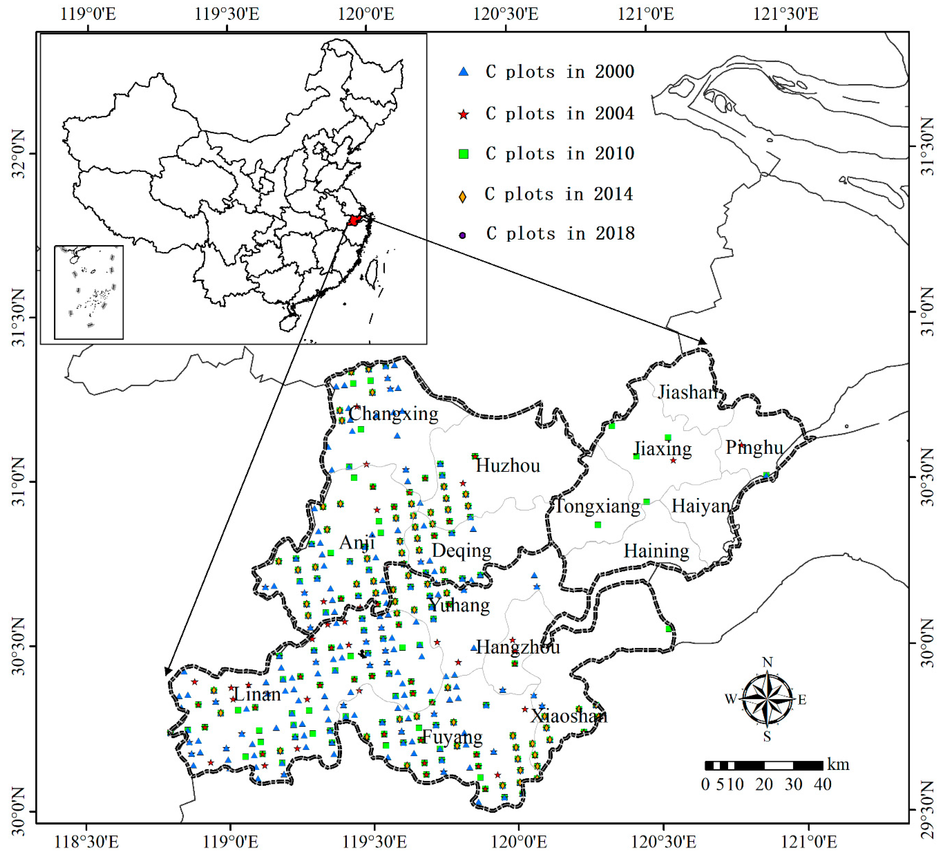
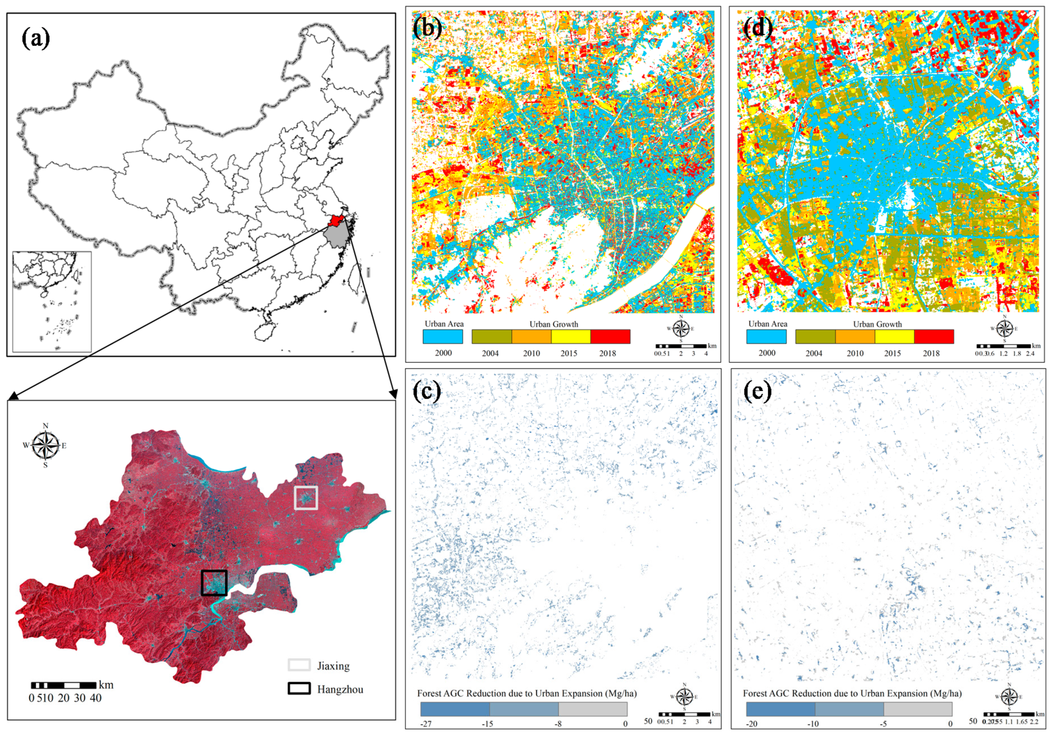
2.1. Study Area

Hang-Jia-Hu is located in the northwestern part of Zhejiang Province, China, ranging from 118°50′15′′ E to 121°19′6′′ E and from 29°42′52′′ N to 31°11′53′′ N (Figure 1). Its climate is subtropical monsoon and the annual average temperature is 15–18 °C, with an average annual precipitation of about 1100 mm. The 18.1 million hectares study area administratively covered the entire Huzhou City and Jiaxing City and the northeastern part of Hangzhou City. Most forest in this place is distributed in the southwest of the study area with the main forest types being broad-leafed forest (BLF), coniferous forest (CNF), and bamboo forest (BMF).

2.2. Datasets and Processing

2.2.1. Processing Landsat Times Series Products

30-m multispectral data of Landsat5 TM (2000, 2004, 2010) and Landsat8 OLI (2015, 2018) were downloaded from the United States Geological Survey (USGS). We selected cloud-free images from the years with ground observations for four scenes that cover our study area (Table 1). Few scenes image contain a high amount of cloud, but the region covering the study area is cloudless. Additionally, due to the poor image quality from 2014, we used the images in 2015 to correspond with field data in 2014.
Satellite remote sensed data are easily influenced by water vapor, aerosol, bidirectional reflection, and data transmission, which will result in serious fluctuations of time series data and influence the desired effect in data analysis [50,51]. Therefore, this study applied the Fast line-of-Sight Atmospheric Analysis of Spectral Hypercubes (FLAASH) [52,53,54] to eliminate such atmospheric interference in each image. A digital elevation model (DEM) [55,56] was used to make terrain corrections, as terrain factors may affect the brightness values of original imagery.
In addition to the original image bands, we calculated vegetation indices and texture variables to use as input data to the forest AGC model. The vegetation indices [57,58,59] included in this study included: NDVI (Normalized Difference Vegetation Index), SAVI (Soil Adjusted Vegetation Index), SR (Simple Ratio Index), DVI (Difference Vegetation Index), and EVI (Enhanced Vegetation Index). Additionally, the texture variables based on the gray-level co-occurrence matrix (GLCM) [60,61] included Mean, Variance, Homogeneity, Contrast, Dissimilarity, Entropy, Angular second moment, and Correlation [27,58,59,62,63,64] with different windows (3 × 3, 5 × 5, 7 × 7, 9 × 9, and 11 × 11) [27,65,66]. There were 251 total variables derived with the details that are shown in Table 2.

2.2.2. Processing Observed Data

Forest AGC plots and classification verification plots in 2000, 2004, 2010, and 2014 are all derived from the data of National Forest Inventory (NFI) [20,27] in Zhejiang province. The investigation method of NFI was systematic sampling, which is usually evenly placed at the intersection of kilometer grids of 1:50,000 topographic maps. Each plot size is 28.5 m × 28.5 m. Forest AGC data that were used in 2018 were derived from a field survey in July, 2019. Each plot of 30 m × 30 m was placed to cover a homogenous area of bamboo, inside which the number of trees and average diameter at breast height (DBH) were measured. After calculating the bamboo biomass of each plot by using the growth model, bamboo AGC was calculated by using the conversion coefficients between biomass and carbon stocks. Classification verification data in 2018 were manually and evenly selected from the result of unsupervised classified data and visual interpretation.
Land use in this paper was classified into six types: urban, water, cultivated land (CTL), BLF, CNF, and BMF based on the data of the NFI and field survey [26]. Maximum likelihood [68,69] was applied to make the land use classification map. The classification training samples in this paper are uniformly and evenly selected by the visual interpretation based on the land use spectral reflectance characteristics. The training samples of each land use type were consistent (400 pixels) and they could cover the study area. The total number of classification verification samples in 2000, 2004, 2010, 2014, and 2018 were 171, 175, 191, 156, and 240, respectively, and the numbers of forest verification samples were 120, 116, 137, 106, and 160. Table 3 details forest AGC plots used to construct the AGC estimation model from 2000 to 2018.

2.3. Random Forest and AGC Estimation

Breiman first made formal definition of the RF in 2001, which is a bagging of uncorrelated CART trees learned with randomized node optimization [70,71,72]. First, the algorithm generates N bootstrap samples for the training dataset. Second, a regression tree model is built for each bootstrap sample. Finally, the predicted results are obtained by averaging the predictions from all individual regressions [20]. RF has three important parameters: (1) the number of random regression trees (Ntree); (2) number of variables to be randomly sampled at each node in a tree (Mtry), used to search for the variable that best partitions samples in the training data set and the default number is 1/3 of input variables [73]; and, (3) the minimum number of terminal nodes (Nodesize) where the default value is 5 in regression analysis [8,49].
Forest AGC samples of different years were divided into two groups to optimize the RF model in this study (Table 3), with one group of data accounting for 70% samples represented training samples of the RF model and the remaining 30% represented test samples to test the model accuracy. Training data were also used to evaluate the importance of input variables to forest AGC and select input variables for constructing the RF model. Forest in this paper includes three types and each of them has corresponding forest AGC plots in 2000, 2004, and 2010. In 2014 and 2018, the AGC plots only have the forest type of BMF. Therefore, we decided to use data in 2000, 2004, and 2010 to construct individual AGC estimation models by using the forest non-stratification method [65] and applied the corresponding model to simulate forest AGC in 2000, 2004 and 2010. Subsequently, these three models are applied to predict forest AGC in 2015 and 2018 and the BMF AGC plots in 2014 and 2018 are used for verification. The estimation result in 2015 and 2018 with the highest accuracy in the verification phase will be chosen as the final simulation result. In this paper, we used “RandomForest” package in the R statistical software [74,75] to construct the forest AGC model. During the process of applying the model established, we put the entire image data into the model and run it, and use Python to read the model result into image format, and then perform spatial analysis.

2.4. Accuracy Assessment

The determination coefficient (R2), root mean square error (RMSE), and relative RMSE (RMSEr) [27,65] were used to evaluate the accuracy of the RF model. A higher accuracy is indicated by the higher values of R2 and lower values of RMSE and RMSEr. R2, RMSE, and RMSEr were calculated, as follows:
R 2 = 1 i = 1 n ( p i o i ) 2 / i = 1 n ( o i o i ¯ ) 2
R M S E = 1 n i = 1 n ( p i o i ) 2
R M S E r = R M S E y ¯ × 100
In Equations (1)–(3), R2, RMSE, and RMSEr are the indexes to measure model accuracy; p i and o i are the value of forest AGC samples in the predicted and observed phase in the year of 2000, 2004, and 2010; o i ¯ is the average value of observed plots; y ¯ is the average value of forest AGC in testing samples; and, i is the number of samples.

3. Results

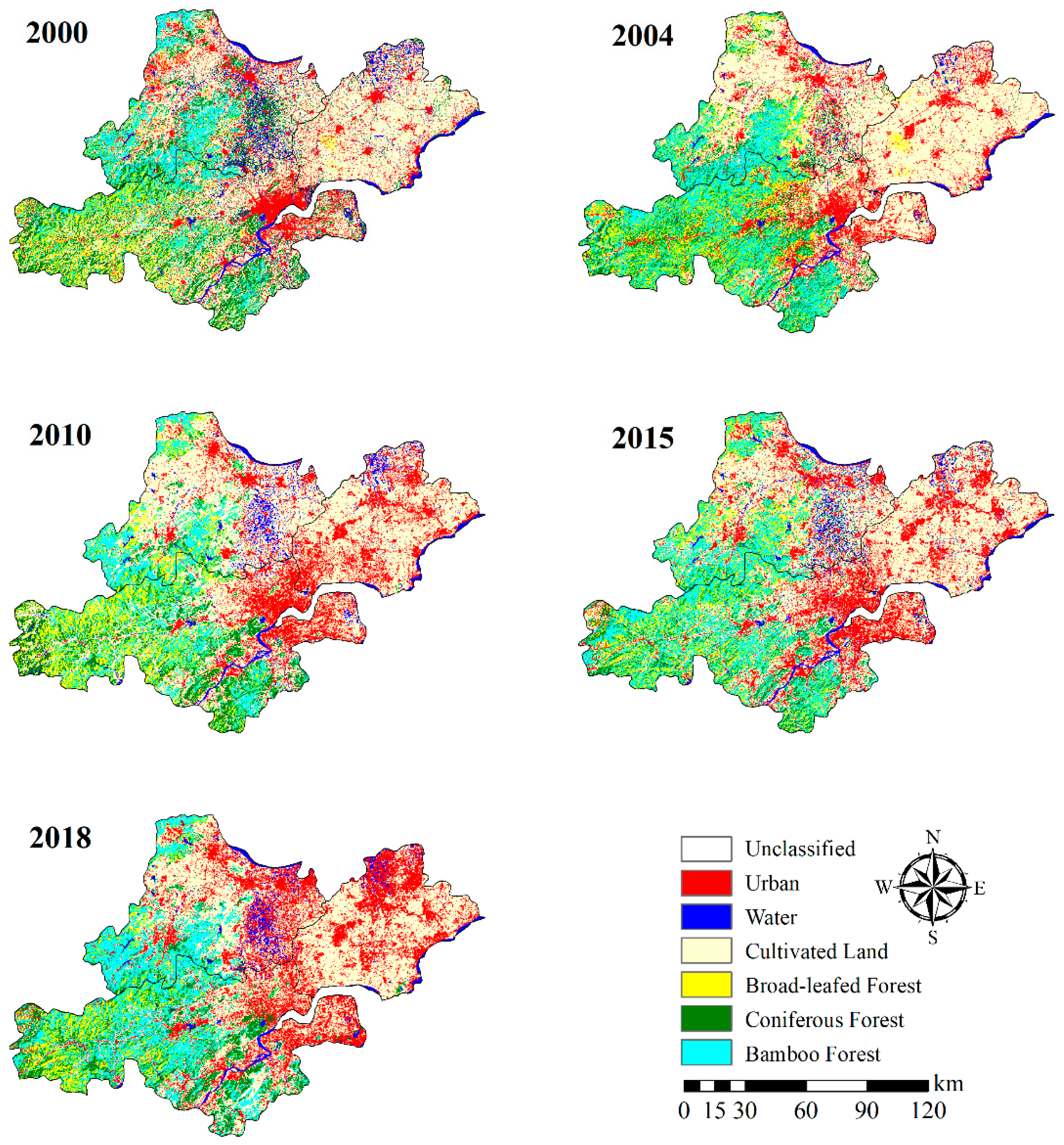
3.1. Land Use Classification

Figure 2 presents the classification results using maximum likelihood methods.
Table 4 shows the overall accuracy of classification by using confusion matrix. It illustrates that the overall classification accuracies in different years were above 86.86%, and the highest was 89.47% with a kappa coefficient above 0.84 and a high of 0.87. The classification accuracies of the BLF, BMF, and CNF were between 86.67% and 89.62%. Classification verification results show a high level of precision. Based on this high precision classification result, we extracted BLF, BMF and CNF separately and use it to mask the forest AGC estimation results.

3.2. RF Model Construction

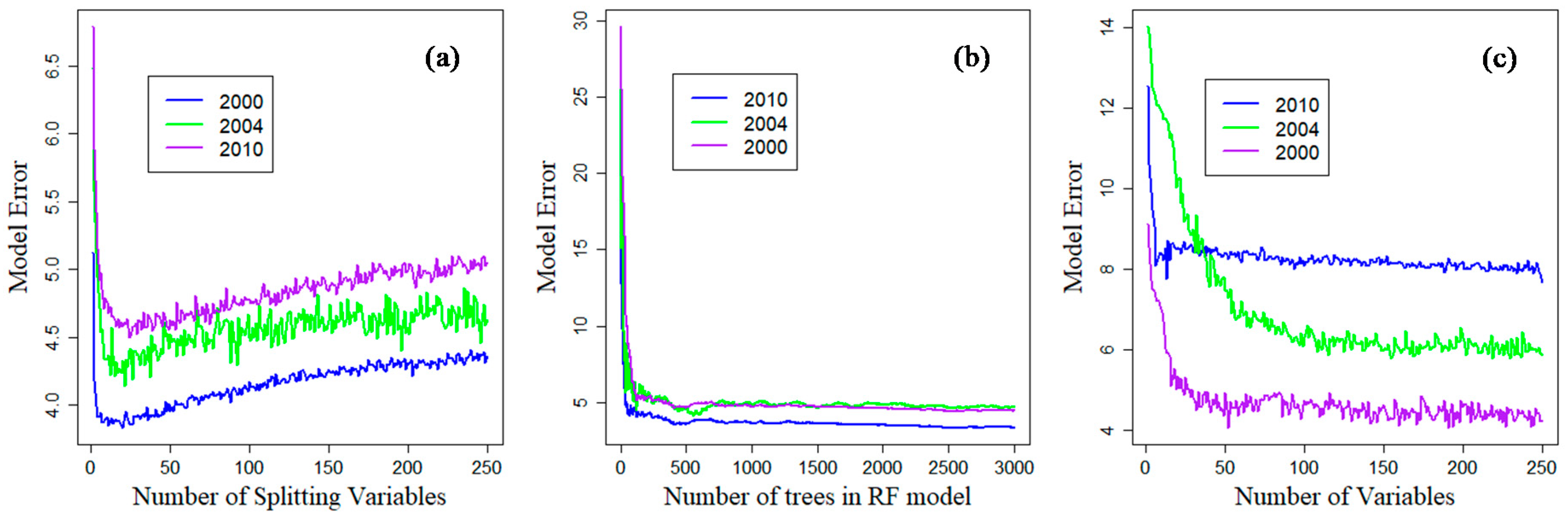
3.2.1. Parameters Optimization of RF

Training data were used to input into RF to traverse all of the variables values and finally obtain the optimal parameters. Figure 3 shows the results. Figure 3a presents Mtry, which is used to determine the minimum amounts of variables in each tree to construct RF. As can be seen from Figure 3a, when Mtry is a certain value, the model error is the smallest, which is the minimum Mtry value that is required. Ntree in Figure 3b shows that model error tends to be stable when the Mtry is big enough. Additionally, we used a 10-fold cross-validation to observe the effect of the number of variables on the model error. Results in Figure 3c represent the variation trend of average model errors in this process. It shows that the variables in the model are not as good as possible. When the model traverses all possibilities, the model error will tend to be stable until a certain amount, when the value of the model error reaches a minimum. Table 5 lists specific settings for different parameter values of different models.

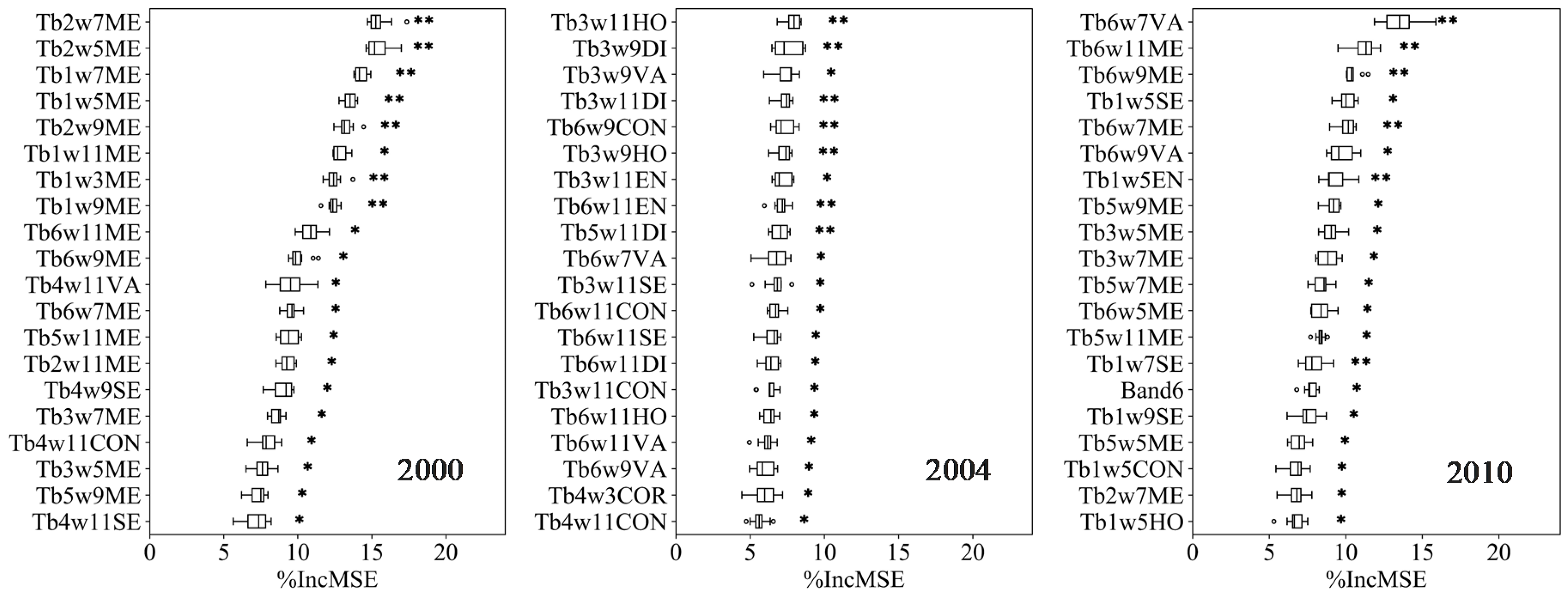
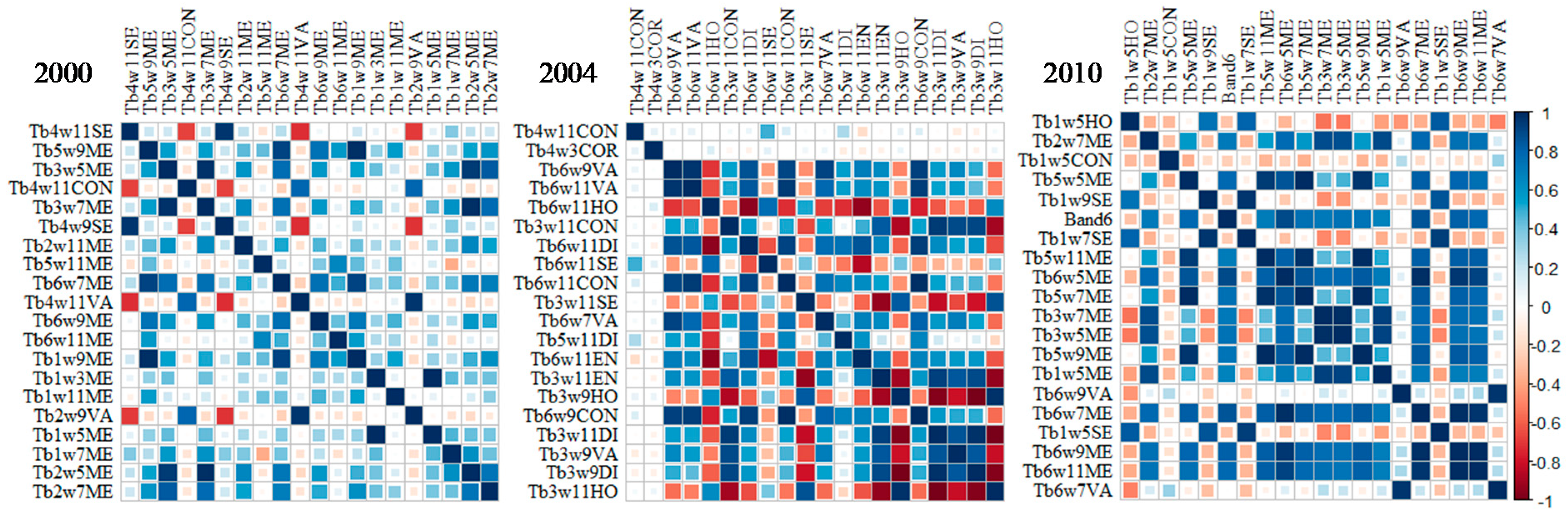
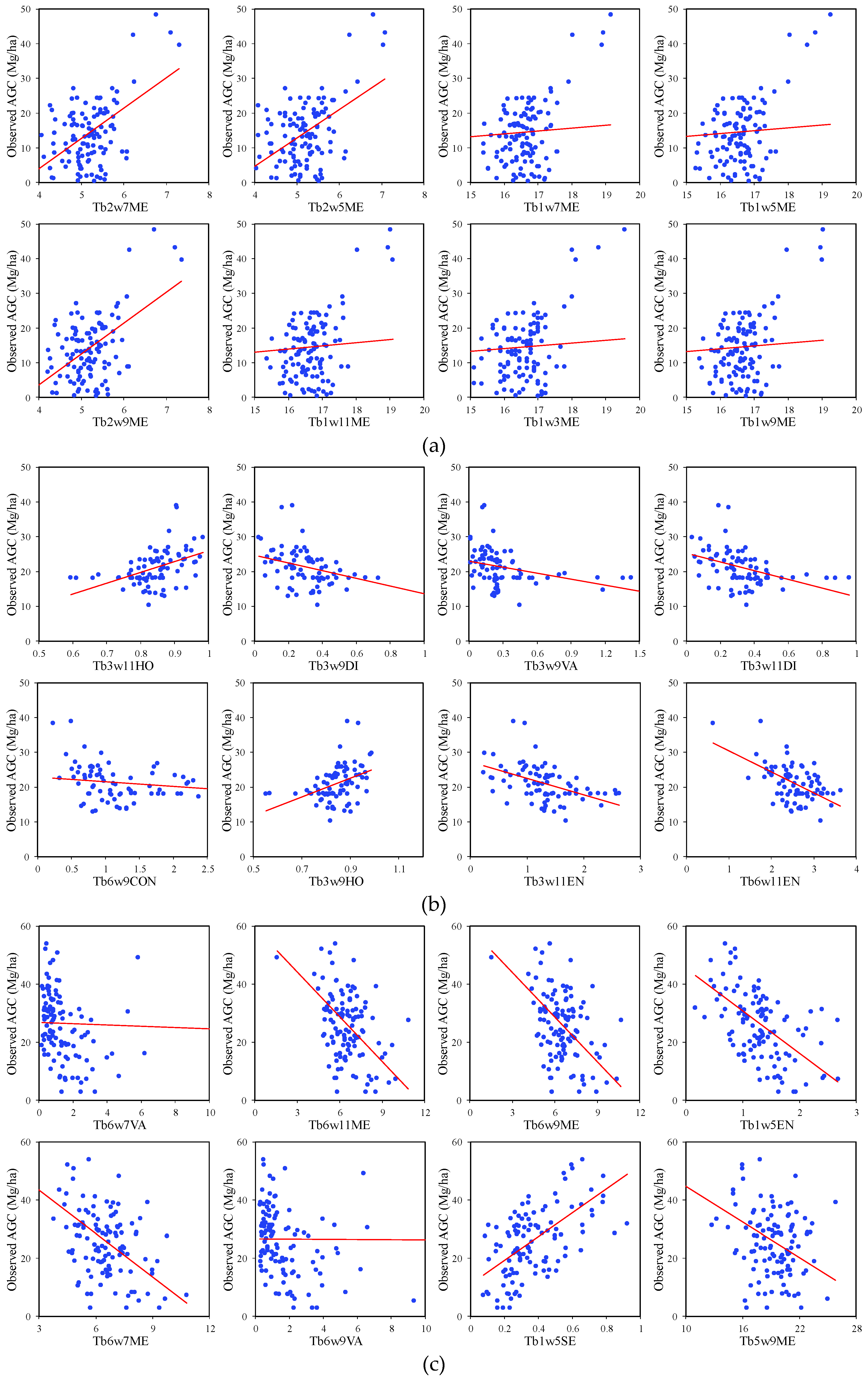
3.2.2. Variable Importance and Autocorrelation

The RF model in different years was ran 100 times each to observe changes in variables importance. We listed the first 20 variables with importance scores of different models in Figure 4. Among all of the variables used in the three models, most of the variables are texture features, while the original band and vegetation index account for a small proportion. Upon viewing of variable selection in different models, we found that 80% of the variables are the mean of the texture features in 2000 model. It reveals that the texture mean at different windows of the original band is important for estimating forest AGC. In the 2004 model, the sixth band of the original band occupies 45% of the overall variables, followed by the third band at 40%. Additionally, the texture window of 11*11 accounts for 65% of the total variables. It illustrated the importance of the texture features of the third and sixth band at 11 × 11 windows to the estimation. In the 2010 model, the mean of the texture features occupies 55% of the total and the sixth band has a selection probability of 35%, which exceeds other variables. As for the importance scores, in the model of 2000, the influence of Tb2w7ME on forest AGC estimation is the largest at an average of 14.83, followed by Tb2w5ME at 14.73. For 2004, Tb311HO has the largest influence of 8.66, followed by Tb3w9DI with score at 8.61. Tb6w7VA has the largest effect on forest carbon prediction at a score of 13.67 and is followed by Tb6w11ME at 12.01.
We calculated the frequency of the top 100 variables in the different RF models to further understand the proportion of variables in the models. In the 2000 RF model, texture information accounted for 92%, of which the fourth band has the most texture information, while the highest window size is w9, and ME accounts for 28.3% of all texture information. Texture information in the 2004 model occupies 98% of the total variables. The number of textures in the third band is up to 24.5%. W7 and ME have a major advantage in terms of window size and texture value. In 2010, 93% of the texture information in the first band accounted for 27.6%, and w7 is also the window with the most selection. The ME value has the same status as the previous two models in selection to establish forest AGC models.
RF, which is widely used to estimate forest parameters while using remote sensing data, can effectively solve the multicollinearity problems of complex variables in traditional statistical regression models [20,76]. Figure 5 shows the collinear relationship between the first 20 variables. A weak correlation indicates that the RF model could solve the collinearity between variables and the overfitting problem to ensure the accuracy of the forest AGC estimation. We selected the optimal number of variables and the optimal variables to build models for different years based on the optimized parameters.

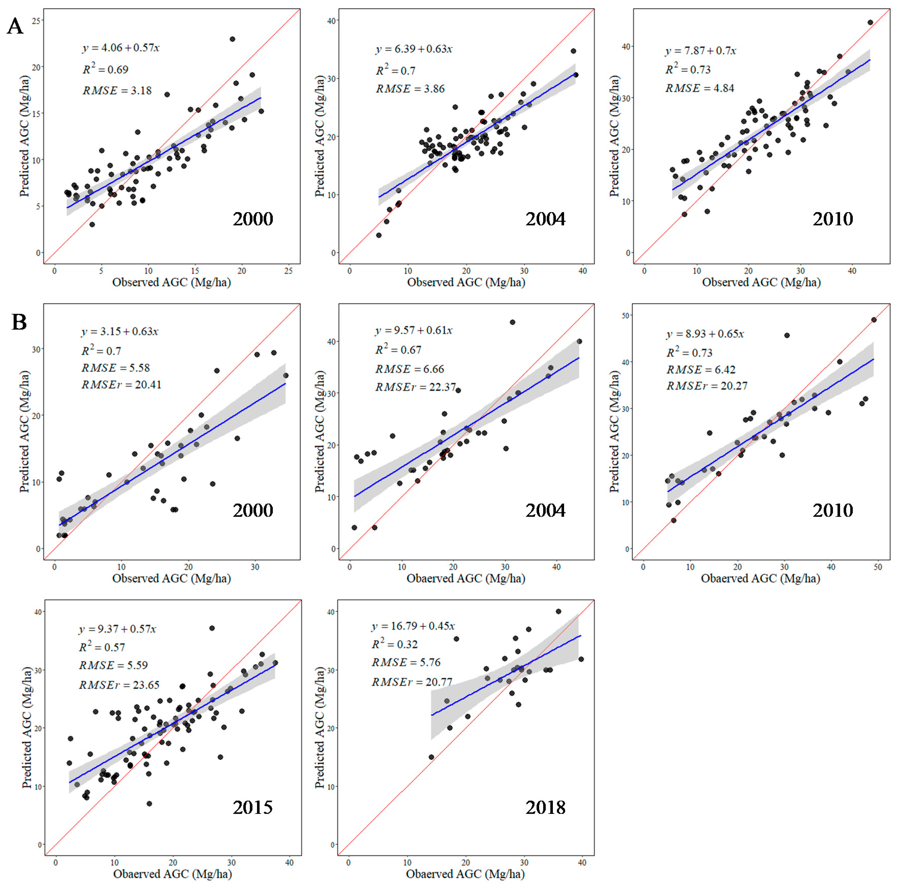
3.3. Estimation and Evaluation of Forest AGC

We extracted the AGC estimation for the forest covers based on the classification results of the maximum likelihood method and simulation results of the RF model established above (Figure 6).
The model performance is evaluated with scatterplots of predicted AGC against the observed data (Figure 7). In the training phase (A) using data from 2000, 2004, and 2010, the models yielded R2 that ranged from 0.69 to 0.73 (p < 0.01) and RMSE from 3.18 Mg/ha to 4.84Mg/ha. In the testing phase (B) of the model in 2000, 2004, and 2010, the R2 value was in the range of 0.67–0.73. RMSE and RMSEr were in the range of 5.58–6.66 Mg/ha and 20.41–23.65. Forest AGC simulation in 2015 and 2018 was done by using the models in 2004 and 2010, respectively. The models yielded an R2 of 0.57 and 0.32. RMSE were 5.59 and 5.76 Mg/ha and RMSEr were 23.65 and 20.77 for 2015 and 2018, respectively.

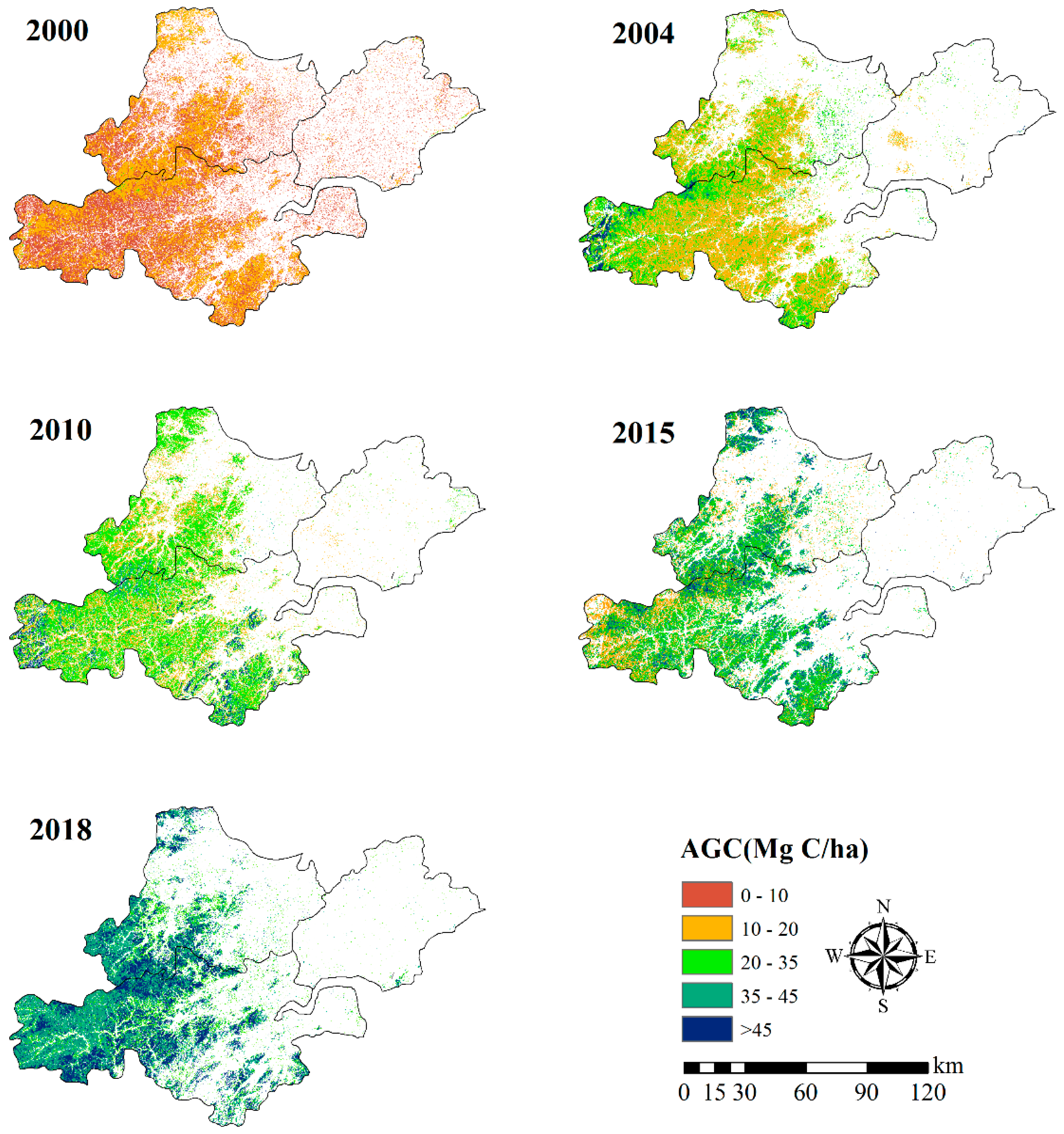
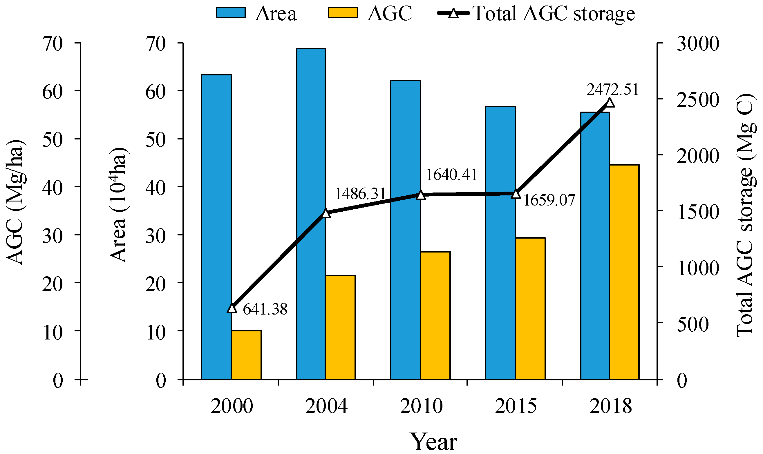
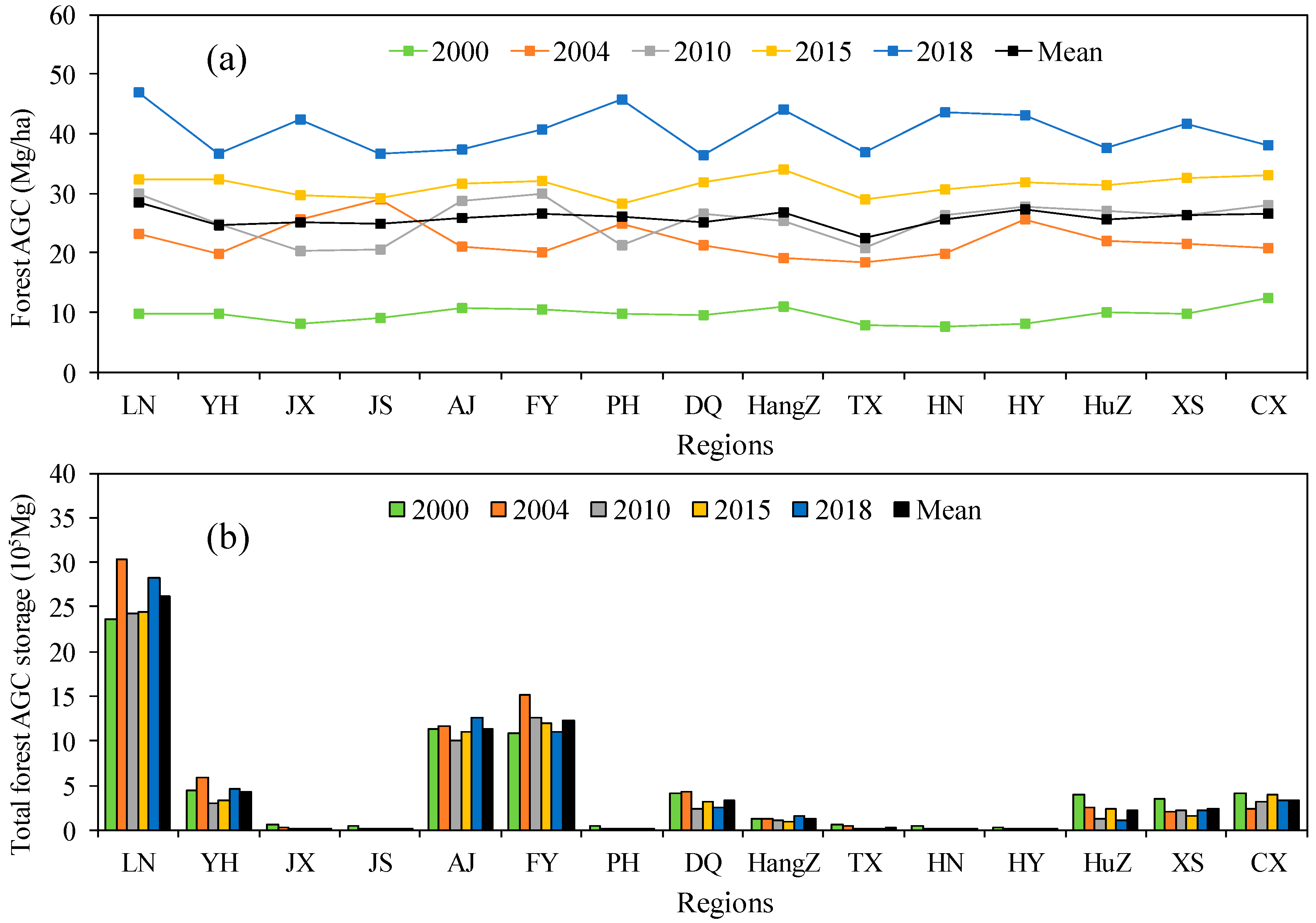
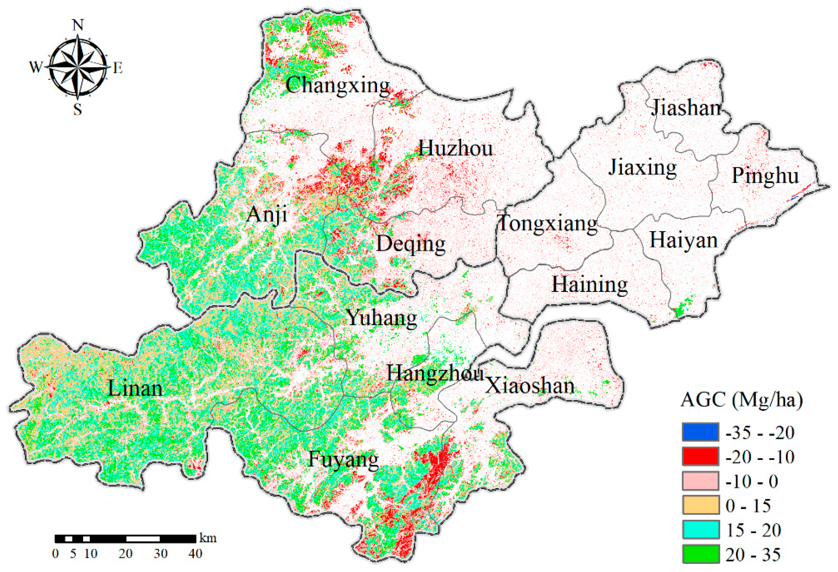
3.4. Spatiotemporal Evolution of Forest AGC

The total forest area in the study region decreased in the past two decades according to the land use classifications in different years. However, forest AGC has gradually increased from 2000 to 2018 in many areas, especially in the west of Hangzhou and southwest of Huzhou. We calculated statistics of forest area, forest AGC, and total AGC storage to understand the change and relationship between forest area, forest AGC, and the total forest AGC storage in Hang-Jia-Hu during the past two dacades (Figure 8). The total forest area only increased from 2000 to 2004 and then gradually decreased afterwards. The total amount of forest area was reduced by 77,713.92 ha with the largest declines occurring following 2004 and 2010. The forest AGC density increased 3.4 times, from 10.14 Mg/ha in 2000 to 44.59 Mg/ha in 2018, and the growth rate was the highest between 2015 and 2018. The total forest AGC storage did not decline due to the reduction of forest area, but it followed the same trend as forest AGC density. It increased from 641.38 Mg C in 2000 to 2472.51 Mg C in 2018, with a growth rate of 285%. This reflects that forest AGC density is more influential on to the total forest AGC storage when compared to the forest area.
Figure 9 shows the interannual variability of forest AGC and total forest AGC storage of 15 sub-regions in Linan (LN), Yuhang (YH), Jiaxing (JX), Jiashan (Js), Anji (AJ), Fuyang (FY), Pinghu (PH), Deqing (DQ), Hangzhou (HangZ), Tongxiang (TX), Hanning (HN), Haiyan (HY), Huzhou (HuZ), Xioashan (XS), and Changxing (CX). Forest AGC did not show obvious variations across different regions (Figure 9a). Forest AGC was the lowest for all subregions in 2000 and the highest in 2018, with the remaining years fluctuating between 22.57 Mg/ha and 28.43 Mg/ha. The total forest AGC varied greatly across subregions mainly due to the variation in forest area. LN, AJ, and FY stood out with over 2 × 10⁶ ha of AGC, while other subregions had less than 1 × 10⁶ ha.
Figure 10 reveals the spatial distribution of forest AGC change from 2000 to 2018. Overall, forest AGC in most of the region is increasing, and the increase is mainly distributed in the western part of the study area. Furthermore, from the above data analysis, forest AGC is increasing during the past two decades. However, some areas showed a decrease in forest AGC, the reduction phenomenon. Such decline in forest AGC mainly occurred near the center of Huzhou and towards the south of Hangzhou in Fuyang District. The magnitude of decline was mainly between −10 Mg/ha and −20 Mg/ha. The reduction of forest AGC in these areas was mounted to 240,660.36 ha.
Moreover, urban forests have received increasing attention in recent years due to their large C sequestration capability and the positive impact on the environment, especially in areas with rapid urban expansion. According to our land use classification, the urban area in the Hang-Jia-Hu region has expanded into suburbs of the cities over the past 20 years, especially around the metropolitan areas, such as Hangzhou and Jiaxing. Extensive decreases of forest AGC were particularly evident in Huzhou City, but not clearly distinguishable in other cities. Therefore, to reveal more details regarding the urban forest AGC change, we used 15-m pan-sharpened Landsat images to analyze the changes of land use in Hangzhou City and Jiaxing City (Figure 11). We found that the urban growth took place in the periphery of Jiaxing and mainly towards the northwest of Hangzhou. In Hangzhou, forest AGC decreased along with intense urban growth in the northwest plains of the City. The decline of forest area due to urbanization reached 3157 ha, which corresponded to an AGC storage loss of 25,309 Mg C. In Jiaxing, forest AGC reduced in all surrounding areas, where the pattern is consistent with the direction of the urban growth. The forest coverage in Jiaxing was reduced by 3078 ha and the forest AGC by 20,701 Mg C as a result of urban growth. It is clearly seen that, although the urban expansion mainly replaced the cultivated lands, it also significantly affected forests.

4. Discussion

In our modeling exercise using RF, we found that land surface texture information is the most important variables of forest AGC. We calculated the correlation between the variables of the corresponding optimal number of variables and forest AGC in different models, and presented a scatter plot of the first eight variables and forest AGC in three models of the training phase to further understand the specific correlation between variables and forest AGC (Figure 12). The results revealed that R2 between the input variables in RF and forest AGC was in the range of 0.13 and 0.32 in the model of 2000, 2004, and 2010. It further reflected that the variables that are involved in RF are closely related with forest AGC, which means that texture information is one of the most essential factors in the process of simulating forest AGC. Furthermore, it also reflected that remote sensing technology, in combination with machine learning algorithms, are an effective means to monitor forest resources in a precise and timely manner at large spatial scales.
However, there are still defects and deficiencies. Firstly, the temporal mismatch of remote sensing and field survey data due to the lack of cloud free Landsat scenes corresponding to the exact times of ground observation can lead to estimation error in the results. Furthermore, different types of forest surfaces have similar spectral signatures, which could have resulted in misclassification [77]. The verification accuracy of the classification results indicates that the BMF is the main reason for the precision declining. Secondly, in the verification phase of simulation results, accuracy in 2015 and 2018 were all below the accuracy in the other three models by a degree. Parameter settings for different modeling due to different raw data vary from year to year. Additionally, different parameter settings will result in the model being only applicable to the simulation of forest AGC in the input data year, but not in other years. Finally, RF also has certain flaws in simulation due to the great requirements for input data. Spatiotemporal distribution of the simulation results show that forest AGC in different periods is concentrated in a certain range (fluctuating around the average of training data), which means that RF has a poor simulation effect on the data at both ends of a dataset, which is consistent with the research result of Gao et al. [65]. High simulation accuracy seems to show that RF is best suited to simulating AGC at certain range, and making the simulation results have the same data distribution as the input data is a critical step. Studies have shown that a combination of multi-source remote sensed data can improve the accuracy of estimation in forest biomass or forest AGC [78]. Furthermore, forest AGC can be simulated with other types of data, such as meteorological data, topography, and soil data [79]. The accuracy of forest AGC simulation can be further improved when considering multivariate remote sensing data and other various impact factors.

5. Conclusions

Based on the remotely sensed and ground survey data, we used the optimized RF models to simulate the distribution patterns and temporal changes of forest AGC in the Hang-Jia-Hu region. Classification by using a maximum likelihood method can present well the land use cover. Additionally, our models estimated forest AGC for the study area in different years with relatively high accuracies. The standardized residuals of the testing samples in different models (Figure 13) are all in the range of −2 to 2, which further illustrates that the optimized RF model has good stability and reliability in predicting forest AGC. With the estimation results, we found that, during the study period from 2000 to 2018, although the total forest area has decreased, the total AGC storage has significantly increased as a result of the increased AGC density. However, forest AGC has decreased near the cities due to the urban expansion in spite of the increase of forest AGC over the entire region.

Author Contributions

Conceptualization, H.D.; Data curation, X.L., L.D., J.Z., H.L., Z.H. and S.H.; Methodology, M.Z.; Supervision, G.Z.; Validation, F.M.; Writing—original draft, M.Z.; Writing—review & editing, H.D.

Funding

The authors gratefully acknowledge the support of the National Natural Science Foundation (No. U1809208, 31670644), the State Key Laboratory of Subtropical Silviculture (No. ZY20180201), the Joint Research fund of Department of Forestry of Zhejiang Province, the Chinese Academy of Forestry (2017SY04), the Zhejiang Provincial Collaborative Innovation Center for Bamboo Resources and High-efficiency Utilization (No. S2017011), and the National Natural Science Foundation (No.31901310).

Acknowledgments

The authors gratefully acknowledge the supports of various foundations. The authors are grateful to the Editor and anonymous reviewers whose comments have contributed to improving the quality.

Conflicts of Interest

The authors declare that they have no competing interests.

References

  1. Federici, S.; Tubiello, F.N.; Salvatore, M.; Jacobs, H.; Schmidhuber, J. New estimates of CO2 forest emissions and removals: 1990–2015. For. Ecol. Manag. 2015, 352, 89–98. [Google Scholar] [CrossRef]
  2. Yan, M.; Tian, X.; Li, Z.; Chen, E.; Wang, X.; Han, Z.; Sun, H. Simulation of Forest Carbon Fluxes Using Model Incorporation and Data Assimilation. Remote. Sens. 2016, 8, 567. [Google Scholar] [CrossRef]
  3. Piao, S.; Fang, J.; Zhu, B.; Tan, K. Forest biomass carbon stocks in China over the past 2 decades: Estimation based on integrated inventory and satellite data. J.Geophys. Res. 2015, 110, 195–221. [Google Scholar] [CrossRef]
  4. Callewaert, P.; Lenders, S.; Gryze, S.D.; Morris, S.J.; Paustian, K. Measuring and Understanding Carbon Storage in Afforested Soils by Physical Fractionation. Soil Sci. Soc. Am. J. 2007, 66, 1981–1987. [Google Scholar]
  5. Santini, N.S.; Adame, M.F.; Nolan, R.H.; Miquelajauregui, Y.; Piñero, D.; Mastretta-Yanes, A.; Cuervo-Robayo, Á.P.; Eamus, D. Storage of organic carbon in the soils of Mexican temperate forests. For. Ecol. Manag. 2019, 446, 115–125. [Google Scholar] [CrossRef]
  6. Lin, B.; Ge, J. Valued forest carbon sinks: How much emissions abatement costs could be reduced in China. J. Clean. Prod. 2019, 224, 455–464. [Google Scholar] [CrossRef]
  7. Pan, Y.; Birdsey, R.A.; Fang, J.; Houghton, R.; Kauppi, P.E.; Kurz, W.A.; Phillips, O.L.; Shvidenko, A.; Lewis, S.L.; Canadell, J.G.; et al. A Large and Persistent Carbon Sink in the World’s Forests. Science 2011, 333, 988–993. [Google Scholar] [CrossRef]
  8. Liu, G.; Bo, F.U.; Fang, J. Carbon dynamics of Chinese forests and its contribution to global carbon balance. Acta Ecol. Sin. 2000, 20, 733–740. [Google Scholar]
  9. Goldewijk, K.K.; Van Minnen, J.G.; Kreileman, G.J.J.; Vloedbeld, M.; Leemans, R.; Minnen, J.G. Simulating the carbon flux between the terrestrial environment and the atmosphere. Water Air Soil Pollut. 1994, 76, 199–230. [Google Scholar] [CrossRef]
  10. Labrecque, S.; Fournier, R.; Luther, J.; Piercey, D. A comparison of four methods to map biomass from Landsat-TM and inventory data in western Newfoundland. For. Ecol. Manag. 2006, 226, 129–144. [Google Scholar] [CrossRef]
  11. Watson, R.T.; Noble, I.R.; Bolin, B.; Ravindranath, N.H.; Verardo, D.J.; Dokken, D.J.; Watson, R.T.; Noble, I.R.; Bolin, B.; Ravindranath, N.H. Land Use, Land-Use Change and Forestry: A Special Report of the Intergovernmental Panel on Climate Change; Cambridge University Press: Cambridge, UK, 2017. [Google Scholar]
  12. Jingyun, F.; Zhaodi, G.; Huifeng, H.; Tomomichi, K.; Hiroyuki, M.; Yowhan, S. Forest biomass carbon sinks in East Asia, with special reference to the relative contributions of forest expansion and forest growth. Glob. Chang. Biol. 2014, 20, 2019–2030. [Google Scholar]
  13. Mitchard, E.T.A. The tropical forest carbon cycle and climate change. Nature 2018, 559, 527–534. [Google Scholar] [CrossRef] [PubMed]
  14. Liu, T.Y.; Mao, F.J.; Li, X.J.; Xing, L.Q.; Dong, L.F.; Zheng, J.L.; Zhang, M.; DU, H. Spatiotemporal dynamic simulation on aboveground carbon storage of bamboo forest and its influence factors in Zhejiang Province, China. J. Appl. Ecol. 2019, 30, 1743–1753. [Google Scholar]
  15. Hai, R.; Hua, C.; Li, L.; Li, P.; Hou, C.; Wan, H.; Zhang, Q.; Zhang, P. Spatial and temporal patterns of carbon storage from 1992 to 2002 in forest ecosystems in Guangdong, Southern China. Plant Soil 2013, 363, 123–138. [Google Scholar]
  16. Heather, K.; Mackey, B.G.; Lindenmayer, D.B. Re-evaluation of forest biomass carbon stocks and lessons from the world’s most carbon-dense forests. Proc. Natl. Acad. Sci. USA 2009, 106, 11635–11640. [Google Scholar]
  17. Chen, L.-C.; Guan, X.; Lib, H.-M.; Wang, Q.-K.; Zhang, W.-D.; Yang, Q.-P.; Wang, S.-L. Spatiotemporal patterns of carbon storage in forest ecosystems in Hunan Province, China. For. Ecol. Manag. 2019, 432, 656–666. [Google Scholar] [CrossRef]
  18. He, B.; Miao, L.; Cui, X.; Wu, Z. Carbon sequestration from China’s afforestation projects. Environ. Earth Sci. 2015, 74, 5491–5499. [Google Scholar] [CrossRef]
  19. Andrews, D. The Carbon Story at the Shale Hills Critical Zone Observatory. In Proceedings of the ASA, CSSA and SSSA International Annual Meeting, Long Beach, CA, USA, 31 October–4 November 2010. [Google Scholar]
  20. Li, X.; Du, H.; Mao, F.; Zhou, G.; Liang, C.; Xing, L.; Fan, W.; Xu, X.; Liu, Y.; Lu, C. Estimating bamboo forest aboveground biomass using EnKF-assimilated MODIS LAI spatiotemporal data and machine learning algorithms. Agric. For. Meteorol. 2018, 256, 445–457. [Google Scholar] [CrossRef]
  21. Mao, F. Construction and Application of Spatiotemporal Carbon Cycle Model of Moso Bamboo Forest Ecosystem. Ph.D. Thesis, Zhejiang A & F University, Hangzhou, China, 2016. [Google Scholar]
  22. Zhao, M.; Yang, J.; Zhao, N.; Liu, Y.; Wang, Y.; Wilson, J.P.; Yue, T. Estimation of China’s forest stand biomass carbon sequestration based on the continuous biomass expansion factor model and seven forest inventories from 1977 to 2013. For. Ecol. Manag. 2019, 448, 528–534. [Google Scholar] [CrossRef]
  23. Li, X.; Mao, F.; Du, H.; Zhou, G.; Xing, L.; Liu, T.; Han, N.; Liu, Y.; Zheng, J.; Dong, L.; et al. Spatiotemporal evolution and impacts of climate change on bamboo distribution in China. Sci. Total Environ. 2019, 248, 109265. [Google Scholar] [CrossRef]
  24. Li, X.; Du, H.; Mao, F.; Zhou, G.; Han, N.; Xu, X.; Liu, Y.; Zheng, J.; Dong, L.; Zhang, M. Assimilating spatiotemporal MODIS LAI data with a particle filter algorithm for improving carbon cycle simulations for bamboo forest ecosystems. Sci. Total Environ. 2019, 694, 133803. [Google Scholar] [CrossRef]
  25. He, L.H.; Wang, H.Y.; Lei, X.D. Parameter sensitivity of simulating net primary productivity of Larix olgensis forest based on BIOME-BGC model. J. Appl. Ecol. 2016, 27, 412. [Google Scholar]
  26. Li, Y.; Du, H.; Mao, F.; Li, X.; Cui, L.; Han, N.; Xu, X. Information extracting and spatiotemporal evolution of bamboo forest based on Landsat time series data in Zhejiang Province. Sci. Silvae Sin. 2019, 55, 88–96. [Google Scholar]
  27. Li, Y.; Ning, H.; Li, X.; Du, H.; Xing, L. Spatiotemporal Estimation of Bamboo Forest Aboveground Carbon Storage Based on Landsat Data in Zhejiang, China. Remote Sens. 2018, 10, 898. [Google Scholar] [CrossRef]
  28. Zhang, J.S.; Pan, Y.Z.; Han, L.J.; Wei, S.U.; He, C.Y. Land Use/cover Change Detection with Multi-source Data. J. Remote Sens. 2007, 11, 500. [Google Scholar]
  29. Hansen, M.C.; Defries, R.S.; Townshend, J.R.G.; Sohlberg, R. Global land cover classification at 1 km spatial resolution using a classification tree approach. Int. J. Remote Sens. 2000, 21, 1331–1364. [Google Scholar] [CrossRef]
  30. Funkenberg, T.; Binh, T.T.; Moder, F.; Dech, S. The Ha Tien Plain—Wetland monitoring using remote-sensing techniques. Int. J. Remote Sens. 2014, 35, 2893–2909. [Google Scholar] [CrossRef]
  31. Ning, H.; Du, H.; Zhou, G.; Xu, X.; Ge, H.; Liu, L.; Gao, G.; Sun, S. Exploring the synergistic use of multi-scale image object metrics for land-use/land-cover mapping using an object-based approach. Int. J. Remote Sens. 2015, 36, 3544–3562. [Google Scholar]
  32. Olofsson, P.; Foody, G.M.; Herold, M.; Stehman, S.V.; Woodcock, C.E.; Wulder, M.A. Good practices for estimating area and assessing accuracy of land change. Remote Sens. Environ. 2014, 148, 42–57. [Google Scholar] [CrossRef]
  33. Horton, A.A.; Walton, A.; Spurgeon, D.J.; Lahive, E.; Svendsen, C. Microplastics in freshwater and terrestrial environments: Evaluating the current understanding to identify the knowledge gaps and future research priorities. Sci. Total Environ. 2017, 586, 127–141. [Google Scholar] [CrossRef] [Green Version]
  34. Chen, Y.; Guerschman, J.P.; Cheng, Z.; Guo, L. Remote sensing for vegetation monitoring in carbon capture storage regions: A review. Appl. Energy 2019, 240, 312–326. [Google Scholar] [CrossRef]
  35. Jia, S.; Shi, S.; Jian, Y.; Lin, D.; Wei, G.; Chen, B.; Song, S. Analyzing the performance of PROSPECT model inversion based on different spectral information for leaf biochemical properties retrieval. ISPRS J. Photogramm. Remote Sens. 2018, 135, 74–83. [Google Scholar]
  36. Graves, S.J.; Caughlin, T.T.; Asner, G.P.; Bohlman, S.A. A tree-based approach to biomass estimation from remote sensing data in a tropical agricultural landscape. Remote Sens. Environ. 2018, 218, 32–43. [Google Scholar] [CrossRef]
  37. Kong, B.; Yu, H.; Du, R.; Wang, Q. Quantitative Estimation of Biomass of Alpine Grasslands Using Hyperspectral Remote Sensing. Rangel. Ecol. Manag. 2019, 72, 336–346. [Google Scholar] [CrossRef]
  38. Wang, S.; Azzari, G.; Lobell, D.B. Crop type mapping without field-level labels: Random forest transfer and unsupervised clustering techniques. Remote Sens. Environ. 2019, 15, 303–317. [Google Scholar] [CrossRef]
  39. Madry, A.; Makelov, A.; Schmidt, L.; Tsipras, D.; Vladu, A. Towards Deep Learning Models Resistant to Adversarial Attacks. arXiv 2017, arXiv:1706.06083. [Google Scholar]
  40. Yang, Q.; Liu, Y.; Chen, T.; Tong, Y. Federated Machine Learning: Concept and Applications. ACM Trans. Intell. Syst. Technol. 2019, 10, 1–19. [Google Scholar] [CrossRef]
  41. Pietquin, O.; Tango, F. A Reinforcement Learning Approach to Optimize the longitudinal Behavior of a Partial Autonomous Driving Assistance System. In Proceedings of the European Conference on Artificial Intelligence, Montpellier, France, 27–31 August 2012. [Google Scholar]
  42. Chen, X.; Ye, C.; Li, J.; Chapman, M.A. Quantifying the Carbon Storage in Urban Trees Using Multispectral ALS Data. IEEE J. Sel. Top. Appl. Earth Obs. Remote Sens. 2018, 11, 1–8. [Google Scholar] [CrossRef]
  43. Duan, M.; Gao, Q.; Wan, Y.; Yue, L.; Guo, Y.; Zhao, G.; Liu, Y.; Qin, X. Biomass estimation of alpine grasslands under different grazing intensities using spectral vegetation indices. Can. J. Remote Sens. 2012, 37, 413–421. [Google Scholar] [CrossRef]
  44. Brilli, L.; Chiesi, M.; Brogi, C.; Magno, R.; Arcidiaco, L.; Bottai, L.; Tagliaferri, G.; Bindi, M.; Maselli, F. Combination of ground and remote sensing data to assess carbon stock changes in the main urban park of Florence. Urban For. Urban Green. 2019, 43, 126377. [Google Scholar] [CrossRef]
  45. Huang, B.F.F.; Boutros, P.C. The parameter sensitivity of random forests. BMC Bioinform. 2016, 17, 331. [Google Scholar] [CrossRef] [PubMed]
  46. Verikas, A.; Gelzinis, A.; Bacauskiene, M. Mining data with random forests: A survey and results of new tests. Pattern Recognit. 2011, 44, 330–349. [Google Scholar] [CrossRef]
  47. Khatami, R.; Mountrakis, G.; Stehman, S.V. A meta-analysis of remote sensing research on supervised pixel-based land-cover image classification processes: General guidelines for practitioners and future research. Remote. Sens. Environ. 2016, 177, 89–100. [Google Scholar] [CrossRef] [Green Version]
  48. Bargiel, D. A new method for crop classification combining time series of radar images and crop phenology information. Remote Sens. Environ. 2017, 198, 369–383. [Google Scholar] [CrossRef]
  49. Chen, L.; Zhou, G.; Du, H.; Liu, Y.; Mao, F.; Xu, X.; Li, X.; Cui, L.; Li, Y.; Zhu, D. Simulaiton of CO2 Flux and Controlling Factors in Moso Bamboo Forest Using Random Forest Algorithm. Sci. Silvae Sin. 2018, 54, 1–12. [Google Scholar]
  50. Gao, B.C.; Montes, M.J.; Davis, C.O.; Goetz, A.F.H. Atmospheric correction algorithms for hyperspectral remote sensing data of land and ocean. Remote Sens. Environ. 2009, 113, S17–S24. [Google Scholar] [CrossRef]
  51. Wei, J.; Lee, Z.; Garcia, R.; Zoffoli, L.; Armstrong, R.A.; Shang, Z.; Sheldon, P.; Chen, R.F. An assessment of Landsat-8 atmospheric correction schemes and remote sensing reflectance products in coral reefs and coastal turbid waters. Remote. Sens. Environ. 2018, 215, 18–32. [Google Scholar] [CrossRef]
  52. Yu, K.; Liu, S.; Zhao, Y. CPBAC: A quick atmospheric correction method using the topographic information. Remote. Sens. Environ. 2016, 186, 262–274. [Google Scholar] [CrossRef]
  53. Guzzi, D.; Barducci, A.; Marcoionni, P.; Pippi, I. An atmospheric correction iterative method for high spectral resolution aerospace imaging spectrometers. In Proceedings of the IEEE International Geoscience and Remote Sensing Symposium, Cape Town, South Africa, 12–17 July 2009. [Google Scholar]
  54. Rani, N.; Mandla, V.R.; Singh, T. Evaluation of atmospheric corrections on hyperspectral data with special reference to mineral mapping. Geosci. Front. 2016, 8, 797–808. [Google Scholar] [CrossRef]
  55. Deng, F.; Rodgers, M.; Xie, S.; Dixon, T.H.; Charbonnier, S.; Gallant, E.A.; Vélez, C.M.L.; Ordoñez, M.; Malservisi, R.; Voss, N.K.; et al. High-resolution DEM generation from spaceborne and terrestrial remote sensing data for improved volcano hazard assessment—A case study at Nevado del Ruiz, Colombia. Remote Sens. Environ. 2019, 233, 111348. [Google Scholar] [CrossRef]
  56. Mapelli, D.; Guarnieri, A.M.M.; Giudici, D. Generation and Calibration of High-Resolution DEM From Single-Baseline Spaceborne Interferometry: The “Split-Swath” Approach. IEEE Trans. Geosci. Remote Sens. 2014, 52, 4858–4867. [Google Scholar] [CrossRef]
  57. Ren, H.; Zhou, G.; Feng, Z. Using negative soil adjustment factor in soil-adjusted vegetation index (SAVI) for aboveground living biomass estimation in arid grasslands. Remote Sens. Environ. 2018, 209, 439–445. [Google Scholar] [CrossRef]
  58. Fatiha, B.; Abdelkader, A.; Latifa, H.; Mohamed, E. Spatio Temporal Analysis of Vegetation by Vegetation Indices from Multi-dates Satellite Images: Application to a Semi Arid Area in ALGERIA. Energy Procedia 2013, 36, 667–675. [Google Scholar] [CrossRef] [Green Version]
  59. Taddeo, S.; Dronova, I.; Depsky, N. Spectral vegetation indices of wetland greenness: Responses to vegetation structure, composition, and spatial distribution. Remote Sens. Environ. 2019, 234, 111467. [Google Scholar] [CrossRef]
  60. Bharati, M.H.; Liu, J.J.; MacGregor, J.F. Image texture analysis: Methods and comparisons. Chemom. Intell. Lab. Syst. 2004, 72, 57–71. [Google Scholar] [CrossRef]
  61. Haralick, R.M. Statistical and structural approaches to texture. Proc. IEEE 1979, 467, 786–804. [Google Scholar] [CrossRef]
  62. Gholizadeh, A.; Zizala, D.; Saberioon, M.; Boruvka, L. Soil Organic Carbon and Texture Retrieving and Mapping using Proximal, Airborne and Sentinel-2 Spectral Imaging. Remote Sens. Environ. 2018, 218, 89–103. [Google Scholar] [CrossRef]
  63. Liu, J.; Pattey, E.; Jégo, G. Assessment of vegetation indices for regional crop green LAI estimation from Landsat images over multiple growing seasons. Remote Sens. Environ. 2012, 123, 347–358. [Google Scholar] [CrossRef]
  64. Calvão, T.; Palmeirim, J.M. Mapping Mediterranean scrub with satellite imagery: Biomass estimation and spectral behaviour. Int. J. Remote Sens. 2004, 25, 3113–3126. [Google Scholar] [CrossRef]
  65. Gao, Y.; Lu, D.; Li, G.; Wang, G.; Qi, C.; Liu, L.; Li, D. Comparative Analysis of Modeling Algorithms for Forest Aboveground Biomass Estimation in a Subtropical Region. Remote Sens. 2018, 10, 627. [Google Scholar] [CrossRef]
  66. Lu, D.; Batistella, M. Exploring TM image texture and its relationships with biomass estimation in Rondônia, Brazilian Amazon. Acta Amaz. 2005, 35, 249–257. [Google Scholar] [CrossRef]
  67. Qi, J.; Chehbouni, A.; Huete, A.R.; Kerr, Y.H.; Sorooshian, S.S. A modified soil adjusted vegetation index. Remote Sens. Envrion. 2015, 48, 119–126. [Google Scholar] [CrossRef]
  68. Hagner, O.; Reese, H. A method for calibrated maximum likelihood classification of forest types. Remote. Sens. Environ. 2007, 110, 438–444. [Google Scholar] [CrossRef]
  69. Cabral, A.I.R.; Silva, S.; Silva, P.C.; Vanneschi, L.; Vasconcelos, M.J. Burned area estimations derived from Landsat ETM+ and OLI data: Comparing Genetic Programming with Maximum Likelihood and Classification and Regression Trees. ISPRS J. Photogramm. Remote Sens. 2018, 142, 94–105. [Google Scholar] [CrossRef]
  70. Breiman, L. Random Forests. Mach. Learn. 2001, 45, 5–32. [Google Scholar] [CrossRef] [Green Version]
  71. Breiman, L. Bagging Predictors. Mach. Learn. 1996, 24, 123–140. [Google Scholar] [CrossRef]
  72. Ao, Y.; Li, H.; Zhu, L.; Ali, S.; Yang, Z. The linear random forest algorithm and its advantages in machine learning assisted logging regression modeling. J. Pet. Sci. Eng. 2018, 174, 776–789. [Google Scholar] [CrossRef]
  73. Brieuc, M.S.O.; Waters, C.D.; Drinan, D.P.; Naish, K.A. A Practical Introduction to Random Forest for Genetic Association Studies in Ecology and Evolution. Mol. Ecol. Resour. 2018, 18, 755–766. [Google Scholar] [CrossRef]
  74. Gounaridis, D.; Koukoulas, S. Urban land cover thematic disaggregation, employing datasets from multiple sources and RandomForests modeling. Int. J. Appl. Earth Obs. Geoinf. 2016, 51, 1–10. [Google Scholar] [CrossRef]
  75. Kai, L.; Yan, E. Co-mention network of R packages: Scientific impact and clustering structure. J. Informetr. 2018, 12, 87–100. [Google Scholar]
  76. Lopatin, J.; Dolos, K.; Hernández, H.J.; Galleguillos, M.; Fassnacht, F.E. Comparing Generalized Linear Models and random forest to model vascular plant species richness using LiDAR data in a natural forest in central Chile. Remote Sens. Environ. 2016, 173, 200–210. [Google Scholar] [CrossRef]
  77. Jiang, X.; Lu, D.; Moran, E.; Calvi, M.F.; Dutra, L.V.; Li, G. Examining impacts of the Belo Monte hydroelectric dam construction on land-cover changes using multitemporal Landsat imagery. Appl. Geogr. 2018, 97, 35–47. [Google Scholar] [CrossRef]
  78. Zhao, P.; Lu, D.; Wang, G.; Liu, L.; Li, D.; Zhu, J.; Yu, S. Forest aboveground biomass estimation in Zhejiang Province using the integration of Landsat TM and ALOS PALSAR data. Int. J. Appl. Earth Obs. Geoinf. 2016, 53, 1–15. [Google Scholar] [CrossRef]
  79. Du, H.; Mao, F.; Zhou, G.; Li, X.; Li, Y. Estimating and Analyzing the Spatiotemporal Pattern of Aboveground Carbon in Bamboo Forest by Combining Remote Sensing Data and Improved BIOME-BGC Model. IEEE J. Sel. Top. Appl. Earth Obs. Remote Sens. 2018, 11, 2282–2295. [Google Scholar] [CrossRef]
Figure 1. Study area and forest aboveground carbon (AGC) plots of different years.
Forests 10 01004 g001
Figure 2. Land use maps from 2000 to 2018.
Forests 10 01004 g002
Figure 3. (a) Influence of Mtry to model error (Mg/ha), (b) Influence of Ntree to model error (Mg/ha), (c) Influence of variables number to model error (Mg/ha).
Forests 10 01004 g003
Figure 4. Importance of the first 20 variables measured in %InMSE (the percentage increase in the mean squared error) from 100 runs of the RF. Note: Tbiwjxx, a texture image developed using the texture measure xx (xx can be such texture measures as ME, VA, HO, CON, DI, EN, SE, COR) on spectral band i (bandi) with a window size of j × j pixel (wj).
Forests 10 01004 g004
Figure 5. Autocorrelation of the first 20 variables in different models.
Forests 10 01004 g005
Figure 6. Spatial distribution of forest AGC from 2000 to 2018.
Forests 10 01004 g006
Figure 7. Accuracy evaluation of RF model at training phase (A) in 2000, 2004, 2010 and testing phase (B) in 2000, 2004, 2010, 2015, and 2018.
Forests 10 01004 g007
Figure 8. Forest area, forest AGC and total forest AGC storage from 2000 to 2018.
Forests 10 01004 g008
Figure 9. (a) Forest AGC of different regions in different years, (b) Total forest AGC storage of different regions in different years.
Forests 10 01004 g009
Figure 10. Spatial distribution change map of forest AGC.
Forests 10 01004 g010
Figure 11. (a) Study area; (b) and (d) urban expansion in the central city of Hangzhou and Jiaxing; and, (c) and (e) forest AGC reduction due to urban expansion in central city of Hangzhou and Jiaxing.
Forests 10 01004 g011
Figure 12. (a) Correlation between the first 8 variables and forest AGC in 2000 model. (b) Correlation between the first 8 variables and forest AGC in 2004 model. (c) Correlation between the first 8 variables and forest AGC in 2010 model.
Forests 10 01004 g012
Figure 13. Standardized residual of the testing phase in different models.
Forests 10 01004 g013
Table 1. Acquisition date and cloud coverage (C) (%) of the Landsat datasets.
WRS2 row/path20002004201020152018
TM 5CTM 5CTM 5COLI 8COLI 8C
11803906/06/20006.1219/07/200414.217/07/20090.0703/08/20154.6815/01/20181.28
11903831/07/20000.1623/05/20040.0324/05/20100.0022/05/201515.423/02/20180.99
11903917/09/20000.0314/10/20040.0024/05/20100.0013/10/20150.6328/04/201812.4
12003910/10/20000.0208/12/20040.0119/08/201011.206/02/201519.919/04/20180.05
Table 2. Information of remote sensing variables.
TypeNameCalculation ModelAbbreviationRemarks
Original BandBand1band1 (band2*)B1Suitable Landsat5 TM (2000, 2004, 2010) and Landsat8 OLI (2015, 2018) data with*
Band2band2 (band3*)B2
Band3band3 (band4*)B3
Band4band4 (band5*)B4
Band5band5 (band6*)B5
Band6band6 (band7*)B6
Vegetation IndexNDVI(B4 − B3)/(B4+B3)NDVIL take value for 0.5 [57,67]
SAVI(B4 − B3)(1 + L)/(B4 + B3 + L)SAVI
EVI2.5 (B4 − B3)/(B4+6B3 − 7.5B1+1)EVI
SRB5/B4SR
DVIB5 − B4DVI
TextureMean i = 0 N 1 j = 0 N 1 i P ( i , j ) ME P ( i , j ) = V ( i , j ) / i = 0 N 1 j = 0 N 1 V ( i , j )
V(i, j) is the ith row of the jth column in the Nth moving window; u x   = j = 0 N 1 j   i = 0 N 1 P ( i , j )
u y   = i = 0 N 1 i   j = 0 N 1 P ( i , j )
σ x   = j = 0 N 1 ( j u i ) 2   i = 0 N 1 P ( i , j )
σ y   = i = 0 N 1 ( i u j ) 2   j = 0 N 1 P ( i , j )
Variance i = 0 N 1 j = 0 N 1 ( i m e a n ) 2 P ( i , j ) VA
Homogeneity i = 0 N 1 j = 0 N 1 P ( i , j ) 1 + ( i j ) 2 HO
Contrast | i j | = 0 N 1 | i j | 2 { i = 1 N j = 1 N P ( i , j ) } CON
Dissimilarity | i j | = 0 N 1 | i j | { i = 1 N j = 1 N P ( i , j ) } DI
Entropy i = 0 N 1 j = 0 N 1 P ( i , j ) log ( P ( i , j ) ) EN
Angular second moment i = 0 N 1 j = 0 N 1 P ( i , j ) 2 SE
Correlation i = 0 N 1 j = 0 N 1 P ( i , j ) 2 μ x μ y σ x σ y COR
Table 3. Summary of the forest AGC plots of different years.
YearSample SizeUnit: Mg/ha
TrainingTestingTotalMinMaxMeanSD
2000160692291.2832.1110.176.02
2004138591974.9238.8420.286.66
2010123521755.3343.4822.899.13
2014-1021022.1837.4917.987.97
2018-424214.0840.8827.265.93
Table 4. Overall accuracy and kappa coefficient of land use classification.
YearOverall Accuracy (%)Forest Extraction Accuracy (%)
Accuracy (%)Kappa Coefficient BLFBMFCNFForest
200089.470.8787.7181.2591.3086.67
200486.860.8490.0086.5488.8788.89
201088.480.8589.1584.8590.9188.57
201589.100.8793.7582.1491.3089.62
201887.900.8692.5085.0090.0089.17
Table 5. Optimized parameters of random forest (RF) models in different years.
YearNodesizeMtryNtreeNumber of Variables
2000520250052
20045212500115
2010524250013

