The Dynamics of Transpiration to Evapotranspiration Ratio under Wet and Dry Canopy Conditions in a Humid Boreal Forest


Abstract
:1. Introduction
2. Materials and Methods
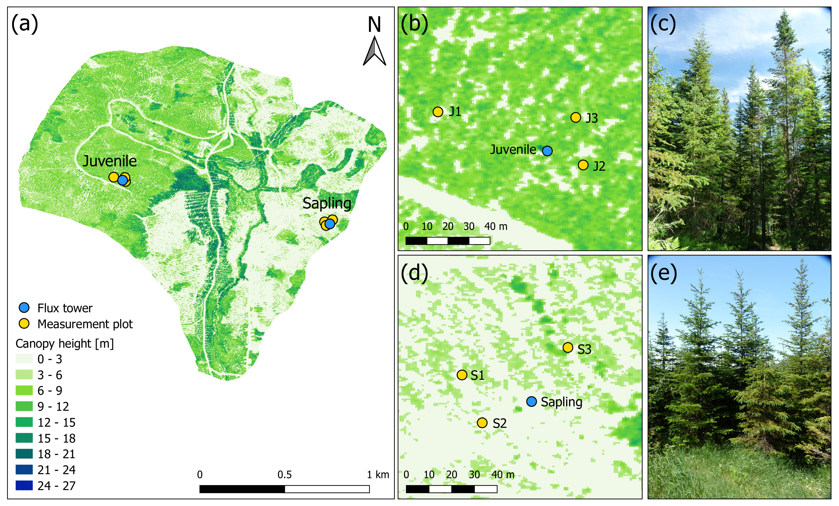
2.1. Study Site
2.2. Eddy-Covariance and Micrometeorological Measurements
2.3. Sap Flow Measurement
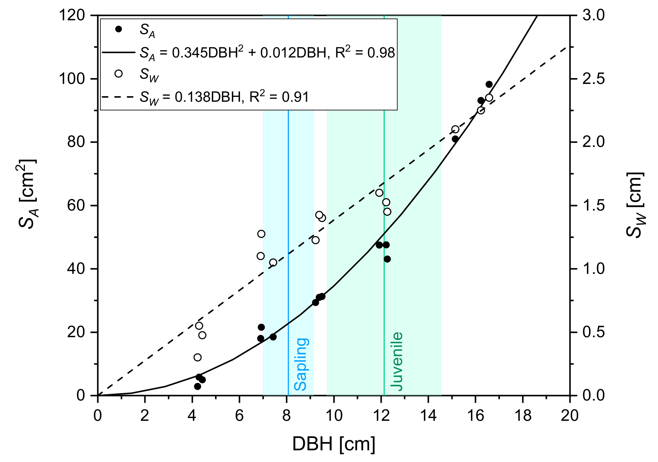
2.4. Species-Specific Calibration of the Thermal Dissipation Approach for Sap Flow Measurements
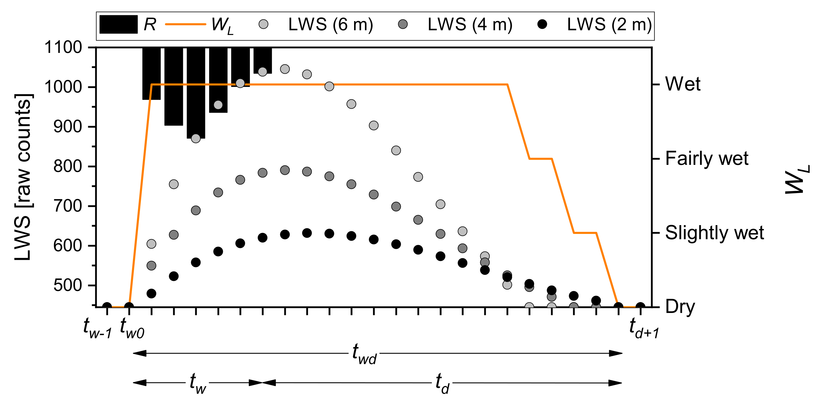
2.5. Monitoring of Canopy Wetness
3. Results
3.1. Determination of
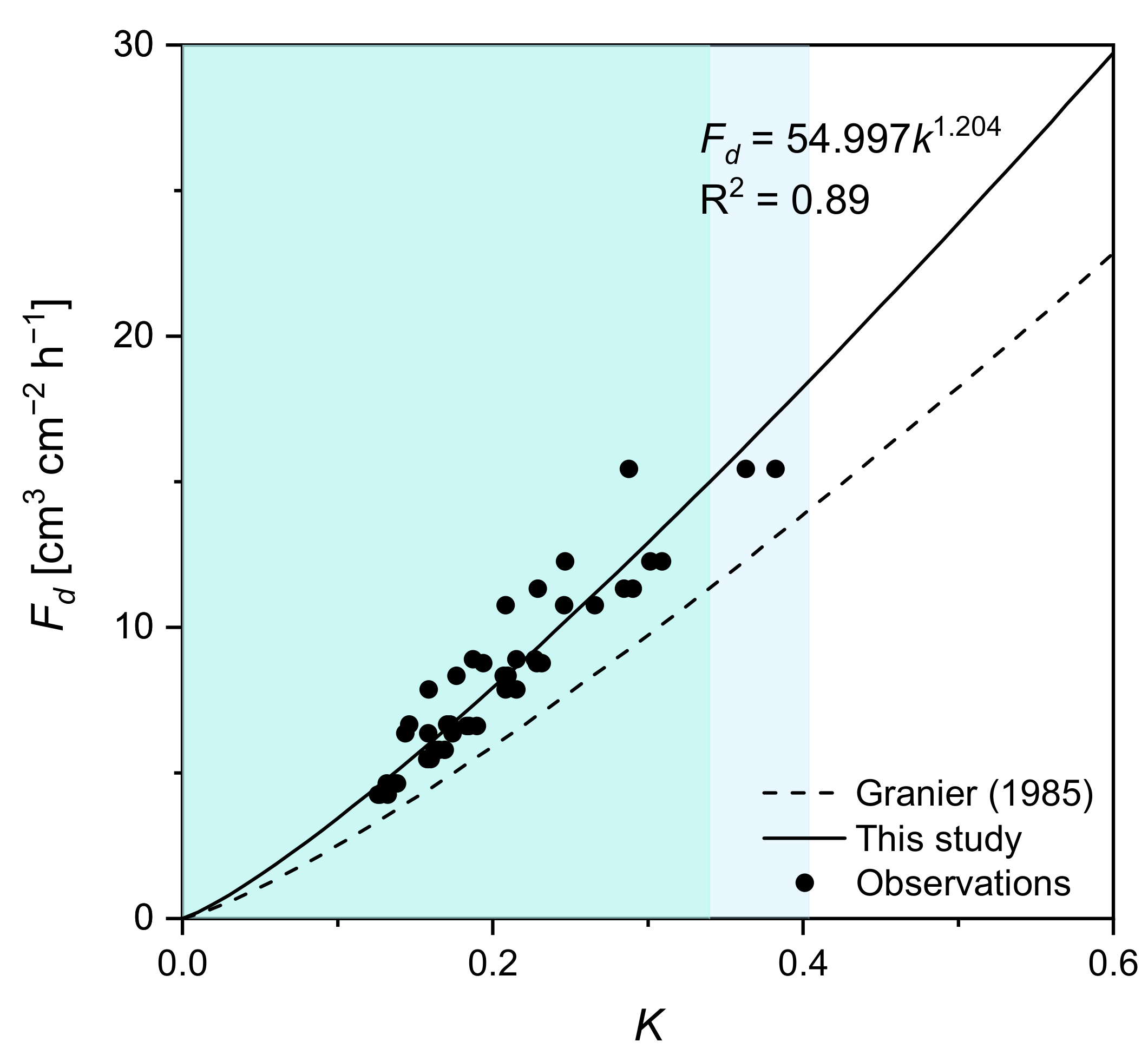
3.1.1. Calibration of Sap Flow Measurements for Balsam Fir
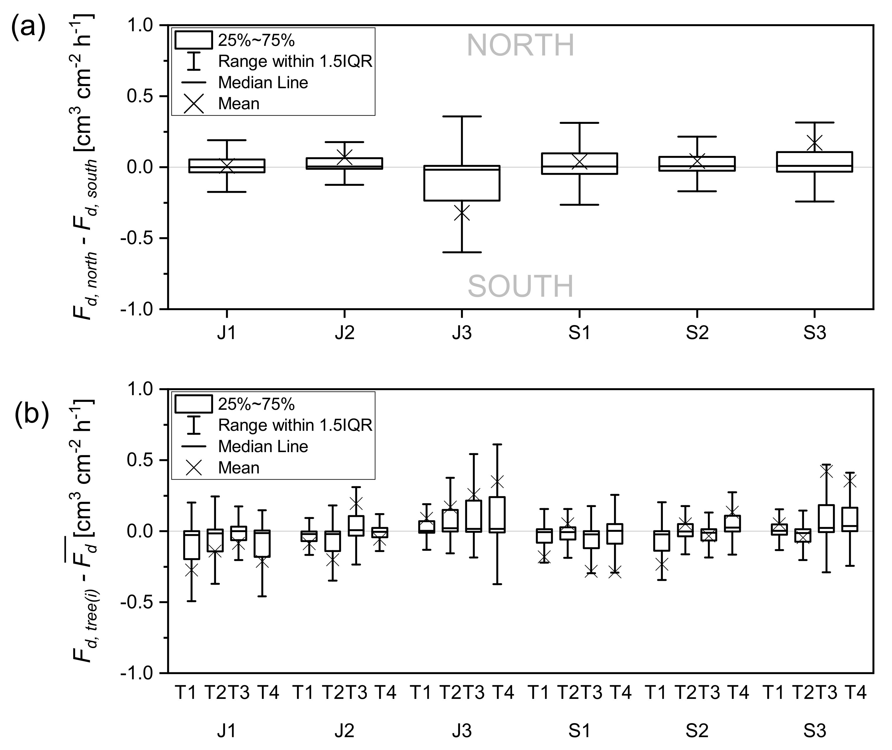
3.1.2. Circumferential and Tree-to-Tree Variations
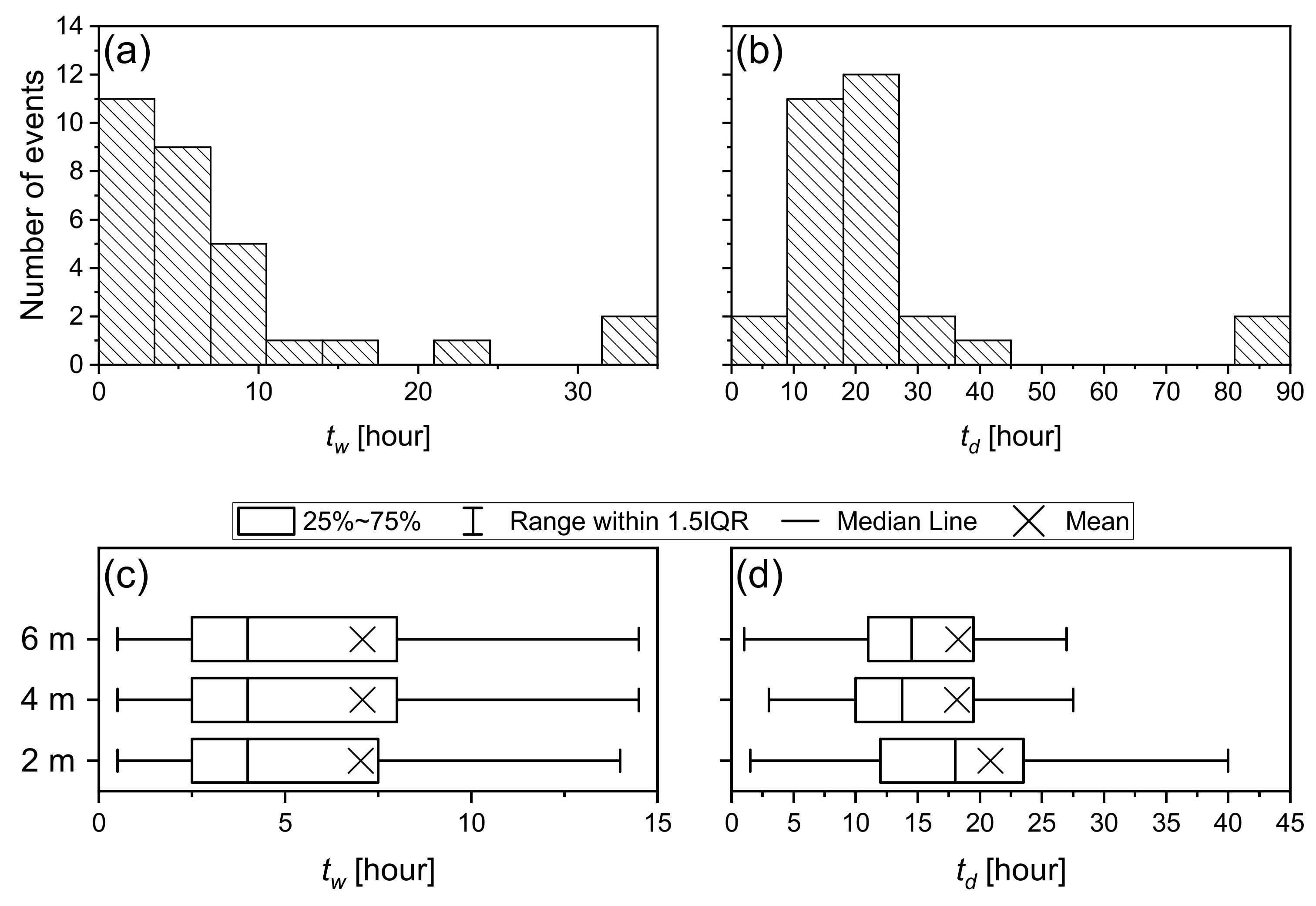
3.2. Characteristics of Wetting–Drying Events
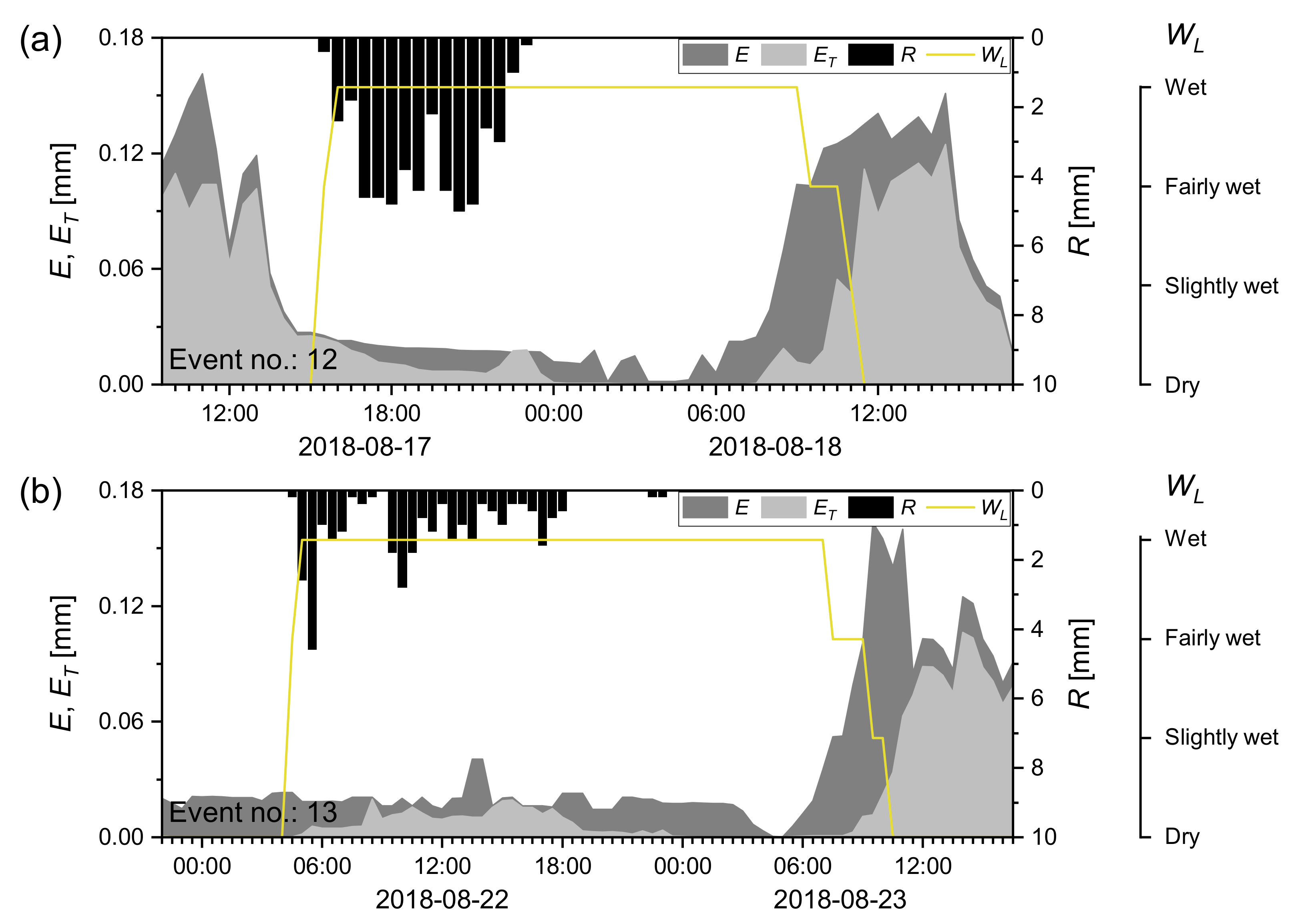
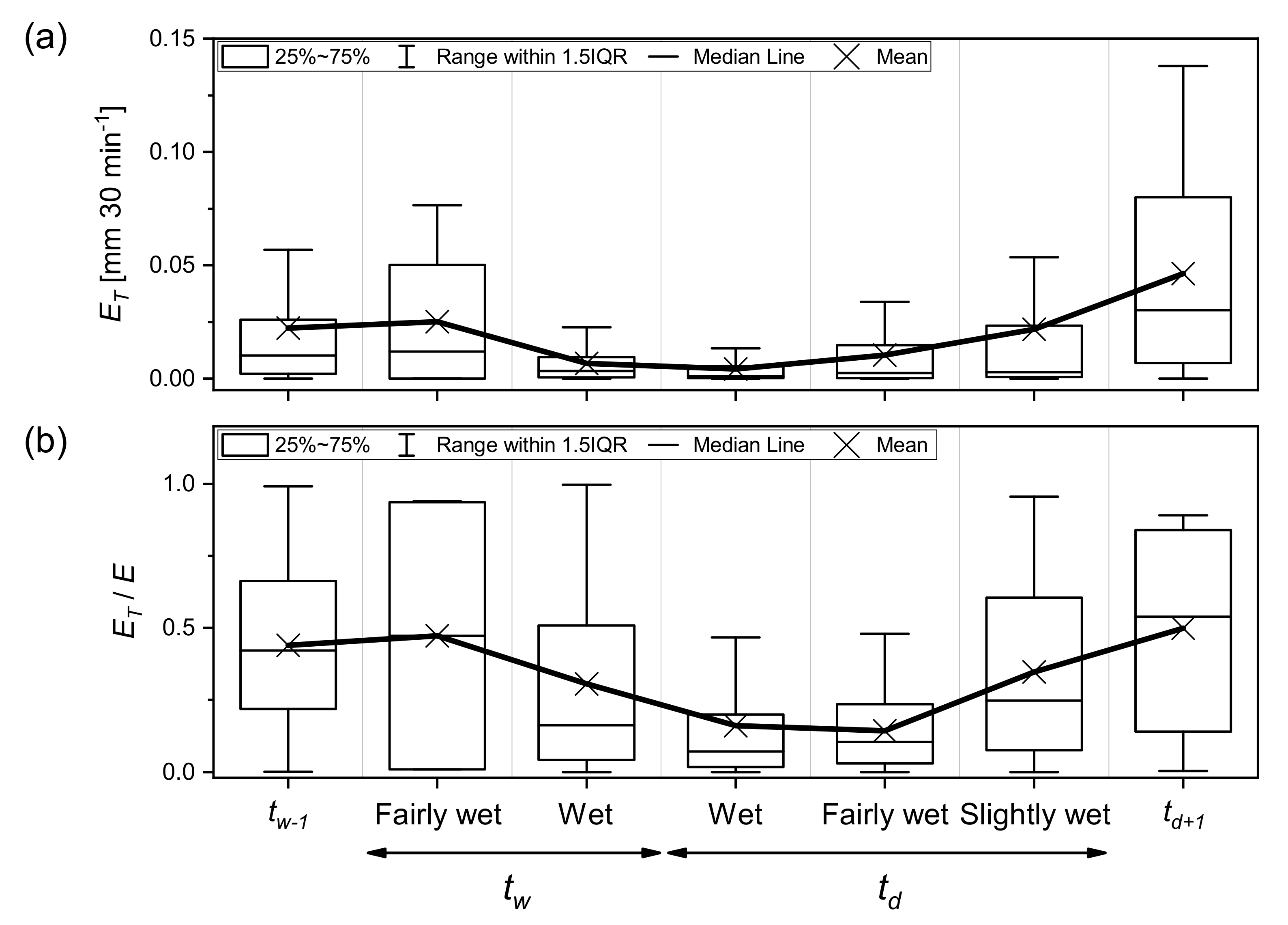
3.3. Dynamics of and during Wetting–Drying Events
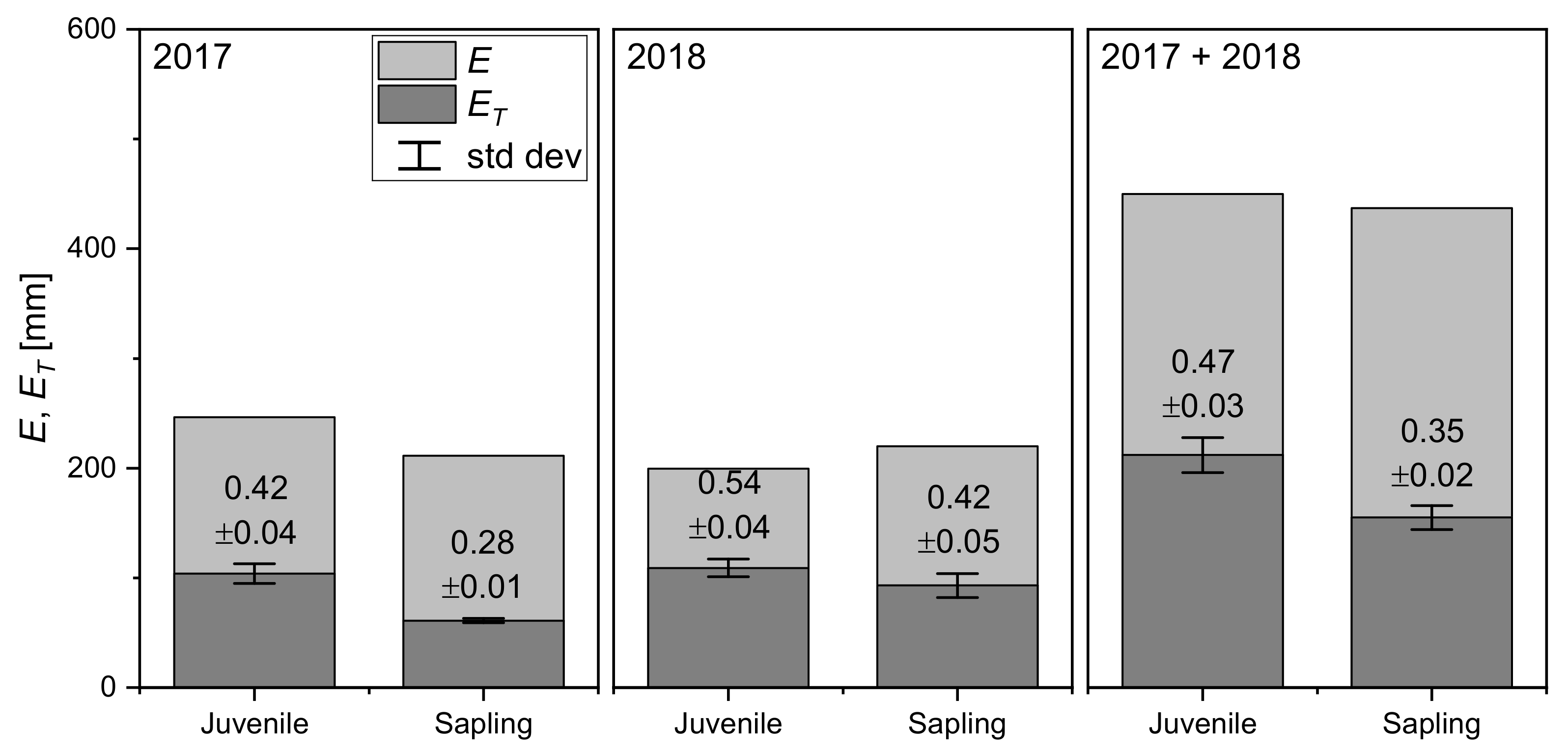
3.4. at the Seasonal Scale
4. Discussion
4.1. Sources of Uncertainty in
4.2. Dynamics of and E during Wetting–Drying Events
4.3. Eddy-Covariance during Rainfall
4.4. at the Seasonal Scale
5. Conclusions
Author Contributions
Funding
Acknowledgments
Conflicts of Interest
Appendix A

| Event | R [mm] | [hour] | [%] | [%] | ||||||
|---|---|---|---|---|---|---|---|---|---|---|
| Slightly Wet [%] | Fairly Wet [%] | Wet [%] | Wet [%] | Fairly Wet [%] | Slightly Wet [%] | |||||
| 1 | 11 | 17 | 15 | 85 | - | - | 100 | 100 | - | - |
| 2 | 7.8 | 35.5 | 23 | 77 | - | - | 100 | 93 | - | 7 |
| 3 | 13.2 | 29 | 14 | 86 | - | - | 100 | 98 | 2 | - |
| 4 | 78.2 | 116.5 | 27 | 73 | - | - | 100 | 91 | 8 | 1 |
| 5 | 4 | 19.5 | 5 | 95 | - | - | 100 | 81 | 19 | - |
| 6 | 16.6 | 15 | 27 | 73 | - | - | 100 | 95 | 5 | - |
| 7 | 3.6 | 28.5 | 9 | 91 | - | - | 100 | 75 | 4 | 21 |
| 8 | 3.8 | 10.5 | 10 | 90 | - | - | 100 | 58 | 21 | 21 |
| 9 | 11.2 | 24.5 | 18 | 82 | - | 11 | 89 | 90 | 5 | 5 |
| 10 | 6 | 21 | 17 | 83 | - | - | 100 | 54 | 29 | 17 |
| 11 | 0.8 | 4 | 13 | 88 | - | - | 100 | 29 | 14 | 57 |
| 12 | 50 | 20 | 40 | 60 | - | 6 | 94 | 83 | 13 | 4 |
| 13 | 31.2 | 30 | 48 | 52 | - | 3 | 97 | 81 | 13 | 6 |
| 14 | 1 | 23.5 | 6 | 94 | - | - | 100 | 82 | 2 | 16 |
| 15 | 4 | 23 | 15 | 85 | - | - | 100 | 67 | 5 | 28 |
| 16 | 8.2 | 20.5 | 12 | 88 | - | - | 100 | 81 | 6 | 14 |
| 17 | 9.4 | 26.5 | 26 | 74 | - | - | 100 | 97 | 3 | - |
| 18 | 1.2 | 19.5 | 5 | 95 | - | - | 100 | 95 | - | 5 |
| 19 | 9 | 13.5 | 22 | 78 | - | - | 100 | 100 | - | - |
| 20 | 5 | 40 | 23 | 78 | - | - | 100 | 87 | 2 | 11 |
| 21 | 12 | 16 | 28 | 72 | - | - | 100 | 65 | 35 | - |
| 22 | 0.6 | 25 | 4 | 96 | 50 | - | 50 | 56 | - | 44 |
| 23 | 27.2 | 25 | 52 | 48 | - | - | 100 | 79 | 13 | 8 |
| 24 | 43.4 | 47 | 50 | 50 | - | - | 100 | 51 | 34 | 15 |
| 25 | 8.8 | 18.5 | 35 | 65 | - | - | 100 | 38 | 17 | 46 |
| 26 | 2.4 | 15 | 17 | 83 | - | - | 100 | 52 | 20 | 28 |
| 27 | 4.6 | 26 | 13 | 87 | - | - | 100 | 53 | 7 | 40 |
| 28 | 6.8 | 44.5 | 10 | 90 | - | 11 | 89 | 34 | 1 | 65 |
| 29 | 69.6 | 114.5 | 29 | 71 | - | - | 100 | 71 | 1 | 28 |
| 30 | 8.6 | 10.5 | 71 | 29 | - | - | 100 | 100 | - | - |
| Time Lag [hour] | All | Dry | Wetting-Drying Events | ||||
|---|---|---|---|---|---|---|---|
| Wetting Phase | Drying Phase | ||||||
| Wet | Fairly Wet | Slightly Wet | |||||
| E [mm 30 min] vs. [mm 30 min] | |||||||
| R | 0 | 0.67 | 0.82 | 0.32 | 0.31 | 0.46 | 0.64 |
| 0.5 | 0.66 | 0.78 | 0.25 | 0.32 | 0.34 | 0.66 | |
| 1 | 0.67 | 0.77 | 0.22 | 0.29 | 0.24 | 0.63 | |
| 1.5 | 0.65 | 0.72 | 0.21 | 0.28 | 0.17 | 0.55 | |
| 2 | 0.61 | 0.65 | 0.20 | 0.22 | 0.15 | 0.48 | |
| Slope | 0 | 0.59 | 0.70 | 0.22 | 0.11 | 0.19 | 0.51 |
| 0.5 | 0.58 | 0.69 | 0.18 | 0.11 | 0.16 | 0.51 | |
| 1 | 0.59 | 0.68 | 0.16 | 0.10 | 0.13 | 0.50 | |
| 1.5 | 0.58 | 0.67 | 0.15 | 0.10 | 0.11 | 0.46 | |
| 2 | 0.57 | 0.65 | 0.14 | 0.09 | 0.08 | 0.43 | |
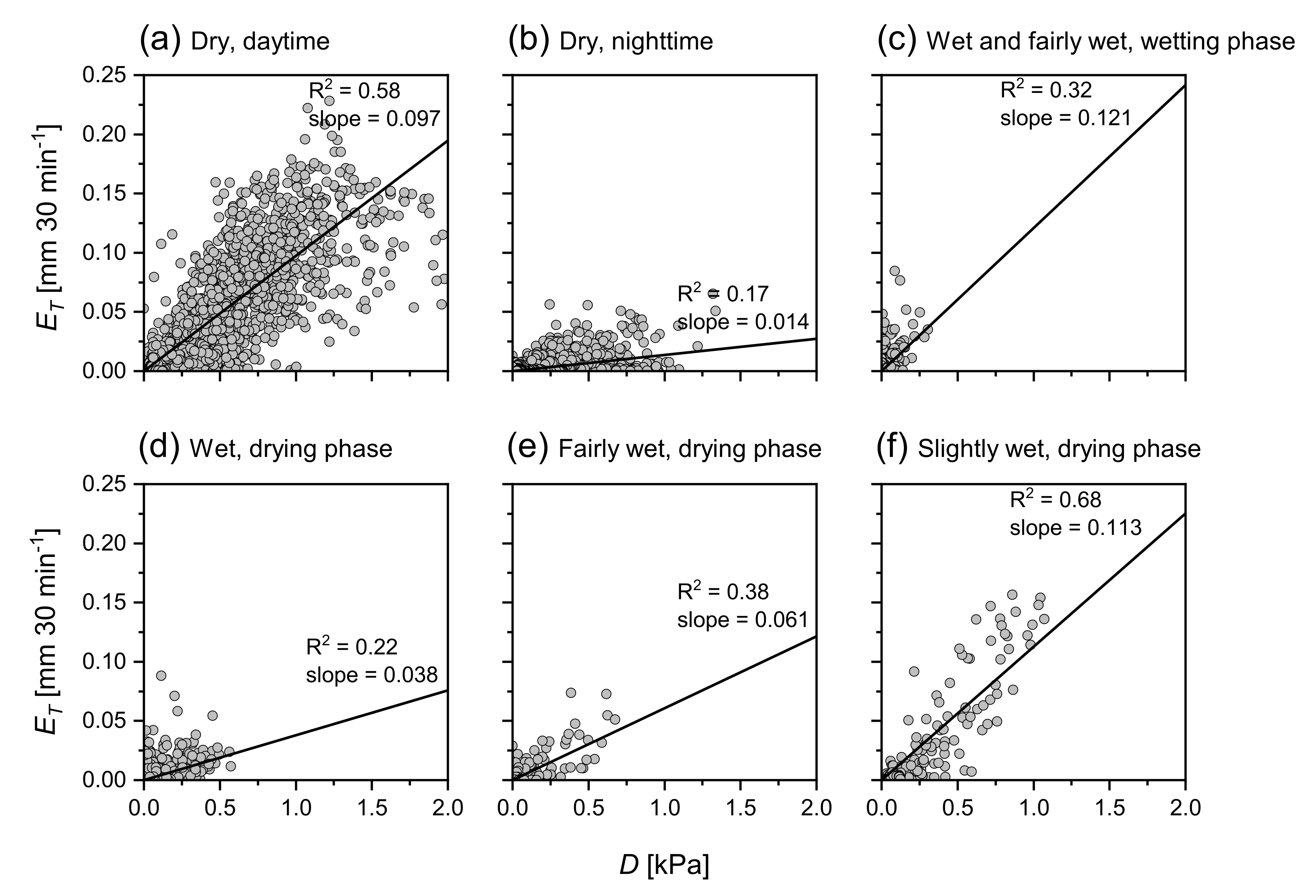
| D [kPa] vs. [mm 30 min] | |||||||
| R | 0 | 0.54 | 0.48 | 0.32 | 0.22 | 0.38 | 0.68 |
| 0.5 | 0.51 | 0.45 | 0.28 | 0.22 | 0.26 | 0.57 | |
| 1 | 0.48 | 0.41 | 0.26 | 0.20 | 0.18 | 0.49 | |
| 1.5 | 0.44 | 0.37 | 0.25 | 0.18 | 0.13 | 0.44 | |
| 2 | 0.39 | 0.33 | 0.24 | 0.17 | 0.13 | 0.41 | |
| Slope | 0 | 0.08 | 0.08 | 0.12 | 0.04 | 0.06 | 0.11 |
| 0.5 | 0.08 | 0.08 | 0.11 | 0.04 | 0.05 | 0.11 | |
| 1 | 0.08 | 0.08 | 0.10 | 0.03 | 0.04 | 0.10 | |
| 1.5 | 0.07 | 0.07 | 0.09 | 0.03 | 0.03 | 0.09 | |
| 2 | 0.07 | 0.07 | 0.09 | 0.03 | 0.03 | 0.09 | |
References
- Dixon, R.K.; Solomon, A.M.; Brown, S.; Houghton, R.A.; Trexier, M.C.; Wisniewski, J. Carbon pools and flux of global forest ecosystems. Science 1994, 263, 185–190. [Google Scholar] [CrossRef] [PubMed]
- Bonan, G.B. Forests and climate change: Forcings, feedbacks, and the climate benefits of forests. Science 2008, 320, 1444–1449. [Google Scholar] [CrossRef] [PubMed] [Green Version]
- Baldocchi, D.; Kelliher, F.M.; Black, T.A.; Jarvis, P. Climate and vegetation controls on boreal zone energy exchange. Glob. Change Biol. 2000, 6, 69–83. [Google Scholar] [CrossRef] [Green Version]
- Kropp, H.; Loranty, M.; Alexander, H.D.; Berner, L.T.; Natali, S.M.; Spawn, S.A. Environmental constraints on transpiration and stomatal conductance in a Siberian Arctic boreal forest. J. Geophys. Res. 2017, 122, 487–497. [Google Scholar] [CrossRef]
- Grelle, A.; Lundberg, A.; Lindroth, A.; Morén, A.-S.; Cienciala, E. Evaporation components of a boreal forest: Variations during the growing season. J. Hydrol. 1997, 197, 70–87. [Google Scholar] [CrossRef]
- IPCC. Contribution of Working Group I to the Fifth assessment report of the Intergovernmental Panel on Climate Change. In Climate Change 2013: The Physical Science Basis; Cambridge University Press: Cambridge, UK; New York, NY, USA, 2013. [Google Scholar]
- Gauthier, S.; Bernier, P.; Kuuluvainen, T.; Shvidenko, A.Z.; Schepaschenko, D.G. Boreal forest health and global change. Science 2015, 349, 819–822. [Google Scholar] [CrossRef]
- Astrup, R.; Bernier, P.Y.; Genet, H.; Lutz, D.A.; Bright, R.M. A sensible climate solution for the boreal forest. Nat. Clim. Chang. 2018, 8, 11–12. [Google Scholar] [CrossRef]
- Kang, S.; Kimball, J.S.; Running, S.W. Simulating effects of fire disturbance and climate change on boreal forest productivity and evapotranspiration. Sci. Total Environ. 2006, 362, 1–3. [Google Scholar] [CrossRef]
- Oishi, A.C.; Oren, R.; Novick, K.A.; Palmroth, S.; Katul, G.G. Interannual invariability of forest evapotranspiration and its consequence to water flow downstream. Ecosystem 2010, 13, 421–436. [Google Scholar] [CrossRef]
- Sun, G.; Noormets, A.; Gavazzi, M.J.; McNulty, S.G.; Chen, J.; Domec, J.-C.; King, J.S.; Amatya, D.M.; Skaggs, R.W. Energy and water balance of two contrasting loblolly pine plantations on the lower coastal plain of North Carolina, USA. For. Ecol. Manag. 2010, 259, 1299–1310. [Google Scholar] [CrossRef]
- Staudt, K.; Serafimovich, A.; Siebicke, L.; Pyles, R.D.; Falge, E. Vertical structure of evapotranspiration at a forest site (a case study). Agric. For. Meteorol. 2011, 151, 709–729. [Google Scholar] [CrossRef]
- Bosveld, F.C.; Bouten, W. Evaluating a model of evaporation and transpiration with observations in a partially wet douglas-fir forest. Bound.-Layer Meteorol. 2003, 108, 365–396. [Google Scholar] [CrossRef]
- Savenije, H.H.G. The importance of interception and why we should delete the term evapotranspiration from our vocabulary. Hydrol. Process. 2004, 18, 1507–1511. [Google Scholar] [CrossRef]
- Ge, Z.-M.; Kellomäki, S.; Zhou, X.; Wang, K.-Y.; Peltola, H.; Väisänen, H.; Strandman, H. Effects of climate change on evapotranspiration and soil water availability in Norway spruce forests in southern Finland: An ecosystem model based approach. Ecohydrology 2013, 6, 51–63. [Google Scholar] [CrossRef]
- Wang, L.; Good, S.P.; Caylor, K.K. Global synthesis of vegetation control on evapotranspiration partitioning. Geophys. Res. Lett. 2014, 41, 6753–6757. [Google Scholar] [CrossRef]
- Schlesinger, W.H.; Jasechko, S. Transpiration in the global water cycle. Agric. For. Meteorol. 2014, 189, 115–117. [Google Scholar] [CrossRef]
- Fatichi, S.; Pappas, C. Constrained variability of modeled T:ET ratio across biomes. Geophys. Res. Lett. 2017, 44, 6795–6803. [Google Scholar] [CrossRef]
- Warren, R.K.; Pappas, C.; Helbig, M.; Chasmer, L.E.; Berg, A.A.; Baltzer, J.L.; Quinton, W.L.; Sonnentag, O. Minor contribution of overstorey transpiration to landscape evapotranspiration in boreal permafrost peatlands. Ecohydrology 2018, 11, 1–10. [Google Scholar] [CrossRef]
- Isabelle, P.-E.; Nadeau, D.F.; Anctil, F.; Rousseau, A.N.; Jutras, S.; Music, B. Impacts of high precipitation on the energy and water budgets of a humid boreal forest. Agric. For. Meteorol. 2020, 280, 107813. [Google Scholar] [CrossRef]
- Cienciala, E.; Lindroth, A.; Čermák, J.; Hällgren, J.E.; Kučera, J. Assessment of transpiration estimates for Picea abies trees during a growing season. Trees 1992, 6, 121–127. [Google Scholar] [CrossRef]
- Aparecido, L.M.T.; Miller, G.R.; Cahill, A.T.; Moore, G.W. Comparison of tree transpiration under wet and dry canopy conditions in a Costa Rican premontane tropical forest. Hydrol. Process. 2016, 30, 5000–5011. [Google Scholar] [CrossRef]
- Granier, A.; Biron, P.; Lemoine, D. Water balance, transpiration and canopy conductance in two beech stands. Agric. For. Meteorol. 2000, 100, 291–308. [Google Scholar] [CrossRef]
- Wilson, K.B.; Hanson, P.J.; Mulholland, P.J.; Baldocchi, D.D.; Wullschleger, S.D. A comparison of methods for determining forest evapotranspiration and its components: Sap-flow, soil water budget, eddy covariance and catchment water balance. Agric. For. Meteorol. 2001, 106, 153–168. [Google Scholar] [CrossRef]
- Giambelluca, T.W.; Ziegler, A.D.; Nullet, M.A.; Truong, D.M.; Tran, L.T. Transpiration in a small tropical forest patch. Agric. For. Meteorol. 2003, 117, 1–22. [Google Scholar] [CrossRef]
- Barbour, M.M.; Hunt, J.E.; Walcroft, A.S.; Rogers, G.N.D.; McSeveny, T.M.; Whitehead, D. Components of ecosystem evaporation in a temperate coniferous rainforest, with canopy transpiration scaled using sapwood density. New Phytol. 2005, 165, 549–558. [Google Scholar] [CrossRef]
- Oren, R.; Phillips, N.; Katul, G.; Ewers, B.E.; Pataki, D.E. Scaling xylem sap flux and soil water balance and calculating variance: A method for partitioning water flux in forests. Ann. For. Sci. 1998, 55, 191–216. [Google Scholar] [CrossRef]
- Lu, P.; Urban, L.; Zhao, P. Granier’s thermal dissipation probe (TDP) method for measuring sap flow in trees: Theory and practice. Acta Bot. Sin. 2004, 46, 631–646. [Google Scholar]
- Oishi, A.C.; Oren, R.; Stoy, P.C. Estimating components of forest evapotranspiration: A footprint approach for scaling sap flux measurements. Agric. For. Meteorol. 2008, 148, 1719–1732. [Google Scholar] [CrossRef] [Green Version]
- Kumagai, T.; Aoki, S.; Nagasawa, H.; Mabuchi, T.; Kubota, K.; Inoue, S.; Utsumi, Y.; Otsuki, K. Effects of tree-to-tree and radial variations on sap flow estimates of transpiration in Japanese cedar. Agric. For. Meteorol. 2005, 135, 110–116. [Google Scholar] [CrossRef]
- Steppe, K.; De Pauw, D.J.W.; Doody, T.M.; Teskey, R.O. A comparison of sap flux density using thermal dissipation, heat pulse velocity and heat field deformation methods. Agric. For. Meteorol. 2010, 150, 1046–1056. [Google Scholar] [CrossRef]
- Kallarackal, J.; Otieno, D.O.; Reineking, B.; Jung, E.-Y.; Schmidt, M.W.T.; Granier, A.; Tenhunen, J.D. Functional convergence in water use of trees from different geographical regions: A meta-analysis. Trees 2013, 27, 787–799. [Google Scholar] [CrossRef]
- Granier, A. Une nouvelle méthode pour la mesure du flux de sève brute dans le tronc des arbres. Ann. For. Sci. 1985, 42, 193–200. [Google Scholar] [CrossRef]
- Granier, A. Mesure du flux de sève brute dans le tronc du Douglas par une nouvelle méthode thermique. Ann. For. Sci. 1987, 44, 1–14. [Google Scholar] [CrossRef] [Green Version]
- Poyatos, R.; Granda, V.; Molowny-Horas, R.; Mencuccini, M.; Steppe, K.; Martínez-Vilalta, J. SAPFLUXNET: Towards a global database of sap flow measurements. Tree Physiol. 2016, 36, 1449–1455. [Google Scholar] [CrossRef] [Green Version]
- Peters, R.L.; Fonti, P.; Frank, D.C.; Poyatos, R.; Pappas, C.; Kahmen, A.; Carraro, V.; Prendin, A.L.; Schneider, L.; Baltzer, J.L.; et al. Quantification of uncertainties in conifer sap flow measured with the thermal dissipation method. New Phytol. 2018, 219, 1283–1299. [Google Scholar] [CrossRef] [PubMed] [Green Version]
- Bush, S.E.; Hultine, K.R.; Sperry, J.S.; Ehleringer, J.R. Calibration of thermal dissipation sap flow probes for ring- and diffuse-porous trees. Tree Physiol. 2010, 30, 1545–1554. [Google Scholar] [CrossRef] [Green Version]
- Sun, H.; Aubrey, D.P.; Teskey, R.O. A simple calibration improved the accuracy of the thermal dissipation technique for sap flow measurements in juvenile trees of six species. Trees 2012, 26, 631–640. [Google Scholar] [CrossRef]
- Bosch, D.D.; Marshall, L.K.; Teskey, R.O. Forest transpiration from sap flux density measurements in a Southeastern Coastal Plain riparian buffer system. Agric. For. Meteorol. 2014, 187, 72–82. [Google Scholar] [CrossRef]
- Clearwater, M.J.; Meinzer, F.C.; Andrade, J.L.; Goldstein, G.; Holbrook, N.M. Potential errors in measurement of nonuniform sap flow using heat dissipation probes. Tree Physiol. 1999, 19, 681–687. [Google Scholar] [CrossRef] [Green Version]
- Nadezhdina, N.; Čermák, J.; Ceulemans, R. Radial patterns of sap flow in woody stems of dominant and understory species: Scaling errors associated with positioning of sensors. Tree Physiol. 2002, 22, 907–918. [Google Scholar] [CrossRef] [Green Version]
- Fiora, A.; Cescatti, A. Diurnal and seasonal variability in radial distribution of sap flux density: Implications for estimating stand transpiration. Tree Physiol. 2006, 26, 1217–1225. [Google Scholar] [CrossRef] [PubMed] [Green Version]
- Saveyn, A.; Steppe, K.; Lemeur, R. Spatial variability of xylem sap flow in mature beech (Fagus sylvatica) and its diurnal dynamics in relation to microclimate. Botany 2008, 86, 1440–1448. [Google Scholar] [CrossRef]
- Rabbel, I.; Diekkrüger, B.; Voigt, H.; Neuwirth, B. Comparing ΔTmax determination approaches for Granier-based sapflow estimations. Sensors 2016, 16, 1–16. [Google Scholar] [CrossRef] [Green Version]
- Čermák, J.; Kučera, J.; Nadezhdina, N. Sap flow measurements with some thermodynamic methods, flow integration within trees and scaling up from sample trees to entire forest stands. Trees 2004, 18, 529–546. [Google Scholar] [CrossRef]
- Kool, D.; Agam, N.; Lazarovitch, N.; Heitman, J.L.; Sauer, T.J.; Ben-Gal, A. A review of approaches for evapotranspiration partitioning. Agric. For. Meteorol. 2004, 184, 56–70. [Google Scholar] [CrossRef]
- Wang, S.; Pan, M.; Mu, Q.; Shi, X.; Mao, J.; Brümmer, C.; Jassal, R.S.; Krishnan, P.; Li, J.; Black, T.A. Comparing evapotranspiration from eddy covariance measurements, water budgets, remote sensing, and land surface models over Canada. J. Hydrometeorol. 2015, 16, 1540–1560. [Google Scholar] [CrossRef] [Green Version]
- Soubie, R.; Heinesch, B.; Granier, A.; Aubinet, M.; Vincke, C. Evapotranspiration assessment of a mixed temperate forest by four methods: Eddy covariance, soil water budget, analytical and model. Agric. For. Meteorol. 2016, 228, 191–204. [Google Scholar] [CrossRef] [Green Version]
- Hogg, E.H.; Black, T.A.; den Hartog, G.; Neumann, H.H.; Zimmermann, R.; Hurdle, P.A.; Blanken, P.D.; Nesic, Z.; Yang, P.C.; Staebler, R.M.; et al. A comparison of sap flow and eddy fluxes of water vapor from a boreal deciduous forest. J. Geophys. Res.: Atmos. 1997, 102, 28929–28937. [Google Scholar] [CrossRef] [Green Version]
- Williams, D.G.; Cable, W.; Hultine, K.; Hoedjes, J.C.B.; Yepez, E.A.; Simonneaux, V.; Er-Raki, S.; Boulet, G.; De Bruin, H.A.R.; Chehbouni, A.; et al. Evapotranspiration components determined by stable isotope, sap flow and eddy covariance techniques. Agric. For. Meteorol. 2004, 125, 241–258. [Google Scholar] [CrossRef]
- Guillemette, F.; Plamondon, A.P.; Prévost, M.; Lévesque, D. Rainfall generated stormflow response to clearcutting a boreal forest: Peak flow comparison with 50 world-wide basin studies. J. Hydrol. 2005, 302, 137–153. [Google Scholar] [CrossRef]
- Senez-Gagnon, F.; Thiffault, E.; Paré, D.; Achim, A.; Bergeron, Y. Dynamics of detrital carbon pools following harvesting of a humid eastern Canadian balsam fir boreal forest. For. Ecol. Manag. 2018, 430, 33–42. [Google Scholar] [CrossRef]
- Tremblay, Y.; Rousseau, A.N.; Plamondon, A.P.; Lévesque, D.; Jutras, S. Rainfall peak flow response to clearcutting 50% of three small watersheds in a boreal forest, Montmorency Forest, Québec. J. Hydrol. 2008, 352, 67–76. [Google Scholar] [CrossRef]
- Tremblay, Y.; Rousseau, A.N.; Plamondon, A.P.; Lévesque, D.; Prévost, M. Changes in stream water quality due to logging of the boreal forest in the Montmorency Forest, Québec. Hydrol. Process. 2009, 23, 764–776. [Google Scholar] [CrossRef]
- Lavigne, M.-P. Modélisation du Régime Hydrologique et de l’impact des Coupes Forestières sur l’écoulement du Ruisseau des Eaux-Volées à l’aide d’HYDROTEL. Master Thesis, Institut National de la Recherche Scientifique—Centre Eau Terre Environnement, Quebec, QC, Canada, 2007. [Google Scholar]
- Noël, P.; Rousseau, A.N.; Paniconi, C.; Nadeau, D.F. Algorithm for delineating and extracting hillslopes and hillslope width functions from gridded elevation data. J. Hydrol. Eng. 2013, 19, 366–374. [Google Scholar] [CrossRef] [Green Version]
- Coyea, M.R.; Margolis, H.A.; Gagnon, R.R. A method for reconstructing the development of the sapwood area of balsam fir. Tree Physiol. 1990, 6, 283–291. [Google Scholar] [CrossRef] [PubMed]
- MELCC. Données du Programme de Surveillance du Climat; Direction générale de la surveillance du climat; Ministère de l’Environnement et de la Lutte contre les Changements Climatiques: Quebec, QC, Canada, 2019.
- Wilczak, J.M.; Oncley, S.P.; Stage, S.A. Sonic anemometer tilt correction algorithms. Bound. Layer Meteorol. 2001, 99, 127–150. [Google Scholar] [CrossRef]
- Reichstein, M.; Falge, E.; Baldocchi, D.; Papale, D.; Aubinet, M.; Berbigier, P.; Bernhofer, C.; Buchmann, N.; Gilmanov, T.; Granier, A.; et al. On the separation of net ecosystem exchange into assimilation and ecosystem respiration: Review and improved algorithm. Global Change Biol. 2005, 11, 1424–1439. [Google Scholar] [CrossRef]
- Dynamax, Inc. TDP Thermal Dissipation Probe User Manual; Dynamax, Inc.: Houston, TX, USA, 1997. [Google Scholar]
- Delzon, S.; Sartore, M.; Granier, A.; Loustau, D. Radial profiles of sap flow with increasing tree size in maritime pine. Tree Physiol. 2004, 24, 1285–1293. [Google Scholar] [CrossRef] [PubMed] [Green Version]
- Lundblad, M.; Lagergren, F.; Lindroth, A. Evaluation of heat balance and heat dissipation methods for sapflow measurements in pine and spruce. Ann. For. Sci. 2001, 58, 625–638. [Google Scholar] [CrossRef] [Green Version]
- Köstner, B. Evaporation and transpiration from forests in Central Europe–relevance of patch-level studies for spatial scaling. Meteorol. Atmos. Phys. 2001, 76, 69–82. [Google Scholar] [CrossRef]
- METER group, Inc. PHYTOS 31 Manual; METER group, Inc.: Pullman, WA, USA, 2018. [Google Scholar]
- Pons, T.L.; Jordi, W.; Kuiper, D. Acclimation of plants to light gradients in leaf canopies: Evidence for a possible role for cytokinins transported in the transpiration stream. J. Exp. Bot. 2001, 52, 1563–1574. [Google Scholar] [CrossRef] [PubMed]
- Cohen, Y.; Cohen, S.; Cantuarias-Aviles, T.; Schiller, G. Variations in the radial gradient of sap velocity in trunks of forest and fruit trees. Plant Soil 2008, 305, 49–59. [Google Scholar] [CrossRef]
- Sato, T.; Oda, T.; Igarashi, Y.; Suzuki, M.; Uchiyama, Y. Circumferential sap flow variation in the trunks of Japanese cedar and cypress trees growing on a steep slope. Hydrol. Res. Lett. 2012, 6, 104–108. [Google Scholar] [CrossRef] [Green Version]
- Komatsu, H.; Shinohara, Y.; Kume, T.; Tsuruta, K.; Otsuki, K. Does measuring azimuthal variations in sap flux lead to more reliable stand transpiration estimates? Hydrol. Process. 2016, 30, 2129–2137. [Google Scholar] [CrossRef]
- Loustau, D.; Domec, J.C.; Bosc, A. Interpreting the variations in xylem sap flux density within the trunk of maritime pine (Pinus pinaster Ait.): Application of a model for calculating water flows at tree and stand levels. Ann. For. Sci. 1998, 55, 29–46. [Google Scholar] [CrossRef]
- Hacke, U.G.; Lachenbruch, B.; Pittermann, J.; Mayr, S.; Domec, J.C.; Schulte, P.J. The hydraulic architecture of conifers. In Functional and Ecological Xylem Anatomy; Hacke, U.G., Ed.; Springer: Cham, Switzerland, 2015. [Google Scholar]
- Shinohara, Y.; Tsuruta, K.; Ogura, A.; Noto, F.; Komatsu, H.; Otsuki, K.; Maruyama, T. Azimuthal and radial variations in sap flux density and effects on stand-scale transpiration estimates in a Japanese cedar forest. Tree Physiol. 2013, 33, 550–558. [Google Scholar] [CrossRef] [Green Version]
- Moon, M.; Kim, T.; Park, J.; Cho, S.; Ryu, D.; Suh, S.; Kim, H.S. Changes in spatial variations of sap flow in Korean pine trees due to environmental factors and their effects on estimates of stand transpiration. J. Mount. Sci. 2016, 13, 1024–1034. [Google Scholar] [CrossRef]
- Ford, C.R.; Hubbard, R.M.; Kloeppel, B.D.; Vose, J.M. A comparison of sap flux-based evapotranspiration estimates with catchment-scale water balance. Agric. For. Meteorol. 2007, 145, 176–185. [Google Scholar] [CrossRef]
- O’Brien, J.J.; Oberbauer, S.F.; Clark, D.B. Whole tree xylem sap flow responses to multiple environmental variables in a wet tropical forest. Plant Cell Environ. 2004, 27, 551–567. [Google Scholar] [CrossRef]
- Kume, T.; Kuraji, K.; Yoshifuji, N.; Morooka, T.; Sawano, S.; Chong, L.; Suzuki, M. Estimation of canopy drying time after rainfall using sap flow measurements in an emergent tree in a lowland mixed-dipterocarp forest in Sarawak, Malaysia. Hydrol. Process. 2006, 20, 565–578. [Google Scholar] [CrossRef]
- Rutter, A.J.; Kershaw, K.A.; Robins, P.C.; Morton, A.J. A predictive model of rainfall interception in forests, 1. Derivation of the model from observations in a plantation of Corsican pine. Agric. Meteorol. 1971, 9, 367–384. [Google Scholar] [CrossRef]
- Saugier, B.; Granier, A.; Pontailler, J.Y.; Dufrene, E.; Baldocchi, D.D. Transpiration of a boreal pine forest measured by branch bag, sap flow and micrometeorological methods. Tree Physiol. 1997, 17, 511–519. [Google Scholar] [CrossRef] [PubMed]
- Tyree, M.T. Hydraulic limits on tree performance: Transpiration, carbon gain and growth of trees. Trees 2003, 17, 95–100. [Google Scholar] [CrossRef] [Green Version]
- Bréda, N.; Granier, A.; Aussenac, G. Effects of thinning on soil and tree water relations, transpiration and growth in an oak forest (Quercus petraea (Matt.) Liebl. Tree Physiol. 1995, 15, 295–306. [Google Scholar] [CrossRef] [PubMed]
- Granier, A.; Loustau, D.; Bréda, N. A generic model of forest canopy conductance dependent on climate, soil water availability and leaf area index. Ann. For. Sci. 2000, 57, 755–765. [Google Scholar] [CrossRef]
- Gigante, V.; Iacobellis, V.; Manfreda, S.; Milella, P.; Portoghese, I. Influences of Leaf Area Index estimations on water balance modeling in a Mediterranean semi-arid basin. Nat. Hazards Earth Syst. Sci. 2009, 9, 979–991. [Google Scholar] [CrossRef] [Green Version]
- Simic, A.; Fernandes, R.; Wang, S. Assessing the impact of leaf area index on evapotranspiration and groundwater recharge across a shallow water region for diverse land cover and soil properties. J. Water Resour. Hydraul. Eng. 2014, 3, 60–73. [Google Scholar]
- Tesemma, Z.K.; Wei, Y.; Peel, M.C.; Western, A.W. Including the dynamic relationship between climatic variables and leaf area index in a hydrological model to improve streamflow prediction under a changing climate. Hydrol. Earth Syst. Sci. 2015, 19, 2821–2836. [Google Scholar] [CrossRef] [Green Version]
- Isabelle, P.-E.; Nadeau, D.F.; Asselin, M.H.; Harvey, R.; Musselman, K.N.; Rousseau, A.N.; Anctil, F. Solar radiation transmittance of a boreal balsam fir canopy: Spatiotemporal variability and impacts on growing season hydrology. Agric. For. Meteorol. 2018, 263, 1–14. [Google Scholar] [CrossRef]
- Shimizu, T.; Kumagai, T.O.; Kobayashi, M.; Tamai, K.; Iida, S.I.; Kabeya, N.; Ikawa, R.; Tateishi, M.; Miyazawa, Y.; Shimizu, A. Estimation of annual forest evapotranspiration from a coniferous plantation watershed in Japan (2): Comparison of eddy covariance, water budget and sap-flow plus interception loss. J. Hydrol. 2015, 522, 250–264. [Google Scholar] [CrossRef]
- Paul-Limoges, E.; Wolf, S.; Schneider, F.D.; Longo, M.; Moorcroft, P.; Gharun, M.; Damm, A. Partitioning evapotranspiration with concurrent eddy covariance measurements in a mixed forest. Agric. For. Meteorol. 2020, 280, 107786. [Google Scholar] [CrossRef]
- Kozii, N.; Haahti, K.; Tor-ngern, P.; Chi, J.; Hasselquist, E.M.; Laudon, H.; Launiainen, S.; Oren, R.; Peichi, M.; Wallerman, J.; et al. Partitioning the forest water balance within a boreal catchment using sapflux, eddy covariance and process-based model. Hydrol. Earth Syst. Sci. Discuss. 2019, 2019, 1–50. [Google Scholar]


| Plot | Tree Density | h | DBH | LAI | |
|---|---|---|---|---|---|
| [Number of Trees per ha] | [m] | [cm] | [m m] | [m m] | |
| Juvenile | |||||
| J1 | 6500 | 10.2 ± 3.2 | 10.2 ± 2.5 | 3.87 | 0.00253 |
| J2 | 5000 | 11.6 ± 3.5 | 11.4 ± 3.8 | 3.35 | 0.00252 |
| J3 | 6750 | 9.5 ± 2.7 | 8.9 ± 2.0 | 3.55 | 0.00223 |
| Sapling | |||||
| S1 | 9250 | 6.3 ± 1.2 | 6.8 ± 1.5 | 3.07 | 0.00157 |
| S2 | 9250 | 5.6 ± 1.1 | 5.6 ± 1.2 | 2.96 | 0.00154 |
| S3 | 6750 | 5.7 ± 1.5 | 4.6 ± 1.0 | 2.58 | 0.00147 |
| Site | Climatic Zone | Vegetation | Study year(s) | LAI | Annual P | Reference | ||
|---|---|---|---|---|---|---|---|---|
| [mm] | [mm y] | |||||||
| Coweeta Basin, US | Temperate | Eastern white pine | 2004–2005 | 9.4–14.2 | 0.55 | 2241 | 0.65 | [74] |
| Kahoku, Japan | Temperate | Japanese cedar, | 2007–2008 | 3.6–5.2 | 0.43 | 2138 | 0.39 | [86] |
| Japanese cypress | ||||||||
| This study (Juvenile) | Boreal | Balsam fir | 2017–2018 | 3.6 | 0.47 | 1583 | 0.45 | |
| This study (Sapling) | Boreal | Balsam fir | 2017–2018 | 2.9 | 0.35 | 1583 | 0.48 | |
| Walker Branch Watershed, US | Temperate | Mixed forest | 1998–1999 | 6 | 0.43 | 1333 | 0.50 | [24] |
| Duke Forest, US | Temperate | Mixed forest | 2002–2005 | 7 | 0.56 | 1146 | 0.56 | [29] |
| Lägeren, Switzerland | Temperate | Mixed forest | 2014–2015 | 1.7–5.5 | 0.74 | 1037 | 0.87 | [87] |
| Vielsalm, Belgium | Temperate | Mixed forest | 2010–2011 | 4.1–5 | 0.68 | 1000 | 0.35 | [48] |
| Krycklan, Sweden | Boreal | Mixed forest | 2016 | 4.4–5.2 | 0.44 | 619 | 0.86 | [88] |
| Norunda, Sweden | Boreal | Norway spruce | 1995 | 4–5 | 0.65 | 527 | 1.29 | [5] |
| Prince Albert Nat. Park, Canada | Boreal | Trembling aspen | 1994 | 2.3 | 0.95 | 463 | 0.89 | [49] |
| Scotty Creek, Canada | Boreal | Black spruce | 2013 | 0.9–0.3 | 0.02 | 390 | 0.76 | [19] |
© 2020 by the authors. Licensee MDPI, Basel, Switzerland. This article is an open access article distributed under the terms and conditions of the Creative Commons Attribution (CC BY) license (http://creativecommons.org/licenses/by/4.0/).
Share and Cite
Hadiwijaya, B.; Pepin, S.; Isabelle, P.-E.; Nadeau, D.F. The Dynamics of Transpiration to Evapotranspiration Ratio under Wet and Dry Canopy Conditions in a Humid Boreal Forest. Forests 2020, 11, 237. https://0-doi-org.brum.beds.ac.uk/10.3390/f11020237
Hadiwijaya B, Pepin S, Isabelle P-E, Nadeau DF. The Dynamics of Transpiration to Evapotranspiration Ratio under Wet and Dry Canopy Conditions in a Humid Boreal Forest. Forests. 2020; 11(2):237. https://0-doi-org.brum.beds.ac.uk/10.3390/f11020237
Chicago/Turabian StyleHadiwijaya, Bram, Steeve Pepin, Pierre-Erik Isabelle, and Daniel F. Nadeau. 2020. "The Dynamics of Transpiration to Evapotranspiration Ratio under Wet and Dry Canopy Conditions in a Humid Boreal Forest" Forests 11, no. 2: 237. https://0-doi-org.brum.beds.ac.uk/10.3390/f11020237