Soil Respiration in Alder Swamp (Alnus glutinosa) in Southern Taiga of European Russia Depending on Microrelief

Abstract

Swamp forests have been insufficiently studied yet in comparison with thoroughly examined carbon pools and greenhouse gas fluxes of peat bogs. This is primarily since the GHGs in swamp forests have huge spatial (due to the developed microrelief) and temporal variations (due to strong fluctuations in the groundwater level (GWL)). This significantly complicates their study, producing ambiguous results, especially in short-term field research. From June to October 2013–2016, we measured soil respiration (R_soil) in an alder swamp using the static chamber method at five microsites: depression (DEP), flat surface (FL), elevations (EL), tussocks (TUS), and near-stem tussocks (STUS). We carried out a computer simulation of the total R_soil for the season based on R_soil measurements, monitoring of GWL, and soil temperature. In 2013–2016, the average R_soil values (mgC m⁻² h⁻¹ ± σ) on DEP, FL, EL, TUS and STUS comprised 54 ± 50, 94 ± 72, 146 ± 89, 193 ± 96, and 326 ± 183, respectively, whereas the total R_soil values for the season (tC ha⁻¹ season⁻¹ ± σ) comprised 2.0 ± 0.5, 3.5 ± 0.5, 5.3 ± 1.6, 5.4 ± 2.7, and 12.6 ± 3.2. According to the results of observations, GWL was at the level of several cm below the soil surface for most of the season. In 2014 and 2015, there were extra dry periods that led to a drop in GWL to a mark of 30–40 cm below the soil surface. Despite their short duration (2–3 weeks), these dry periods can lead to an increase in the total R_soil for the season from 9 to 45% in the TUS–EL–STUS–FL–DEP sequence.

1. Introduction

Peat bogs, covering about 3% of the land surface, contain more carbon (C) than any other terrestrial ecosystem, including forests [1]. At present, C reserves in peat bogs north of 45° N are estimated at 500 Gt [2,3]. Peat bogs have become the object of close study in the context of C balance while the rapid climatic changes in recent decades [4,5,6,7]. The focus of the studies has been directed toward the oligotrophic bogs, which are most widespread in the boreal zone [8,9,10]. The rate of peat accumulation, the age of the peat deposit [11,12,13], greenhouse gas fluxes [14,15,16], and other aspects of their formation and functioning have been thoroughly studied. Other types of wetlands, such as swamp forests and eutrophic bogs, are also of significant interest. However, in contrast to oligotrophic bogs, they have more heterogeneous both in space and in time physicochemical (richness of nutrients, acidity, redox conditions) and hydrological (periodic flooding and drying) characteristics, which significantly complicates their study and leads to ambiguous results, especially in short-term field studies. The high trophicity of eutrophic bogs can lead to higher and longer carbon dioxide (CO₂) emissions because of soil respiration (R_soil), while swamp forests can occupy significant areas (in Russia, up to 24 million ha [17]) and thus make a significant contribution to the carbon balance of wetland ecosystems of the boreal zone.

Swamp forests dominated by the black alder Alnus glutinosa (L.) Gaertn. in the tree layer are widespread in the European part of Russia, especially in the north of the Russian Plain. Black alder forests occupy 0.9 million ha of this territory [18]. The northern border of their distribution runs through central Karelia (middle taiga) [19], and the southern border reaches the forest-steppe zone [20]. Black alder forests spread from the western border of Russia to the Ural Mountains [21] and further in the Trans-Urals to Tobol [18].

In addition to Russia, black alder forests grow predominantly in Belarus, occupying an area of 660 thousand ha [22], in Ukraine on 130 thousand ha [23], and to a certain extent in Lithuania, Latvia [24], and Estonia [25,26]. They are also found in Poland [27], North America [28,29], and Germany [30]. They usually occupy small (up to 200 ha [20]) areas and are associated with habitats such as the foothills of slopes and near-terrace floodplains of rivers, riverbanks, lakes, and bog shores. They grow in places with abundant flow-through moistening and represent one of the stages of eutrophic swamping. Black alder forests are found in both swamps and dry habitats, with mesophilic species in the grass layer [31].

A large number of publications are devoted to the characteristics of black alder forest swamps, conditions of their formation, geographical distribution, geomorphological predisposition, structure and species diversity of plant communities [19,23,31,32,33,34,35,36,37], etc. However, there are few publications on the role of black alder forest swamps in the cycle of the main biogenic elements in the carbon cycle [26,27,28,29,30].

The study of the components of the current carbon balance of black alder swamps is rather difficult because their water–mineral supply is comprised of waters of various genetic categories. It is difficult to establish the boundaries of catchment areas and consider all categories of waters supplying them, which makes it difficult to determine the runoff from these swamps—one of the expendable elements of the carbon balance. On the contrary, the research on fluxes of carbon-containing greenhouse gases from oligotrophic and mesotrophic (forested and open) swamps is reflected in sufficient detail in publications on the southern and middle taiga of western Siberia and the southern taiga of European Russia [38,39,40,41,42,43,44,45]. At the same time, the black alder swamps located there have not been studied at all in relation to the GHG emissions. This also applies to the soil CO₂ emission (soil respiration—R_soil), which is one of the most sensitive and informative indicators of the carbon balance of biogeocenosis [41].

The aim of this work was to assess soil respiration and its seasonal and annual variation in the tall-grass-fern black alder forest considering the following environmental characteristics: heterogeneity of the microrelief, soil temperature, and groundwater level.

2. Materials and Methods

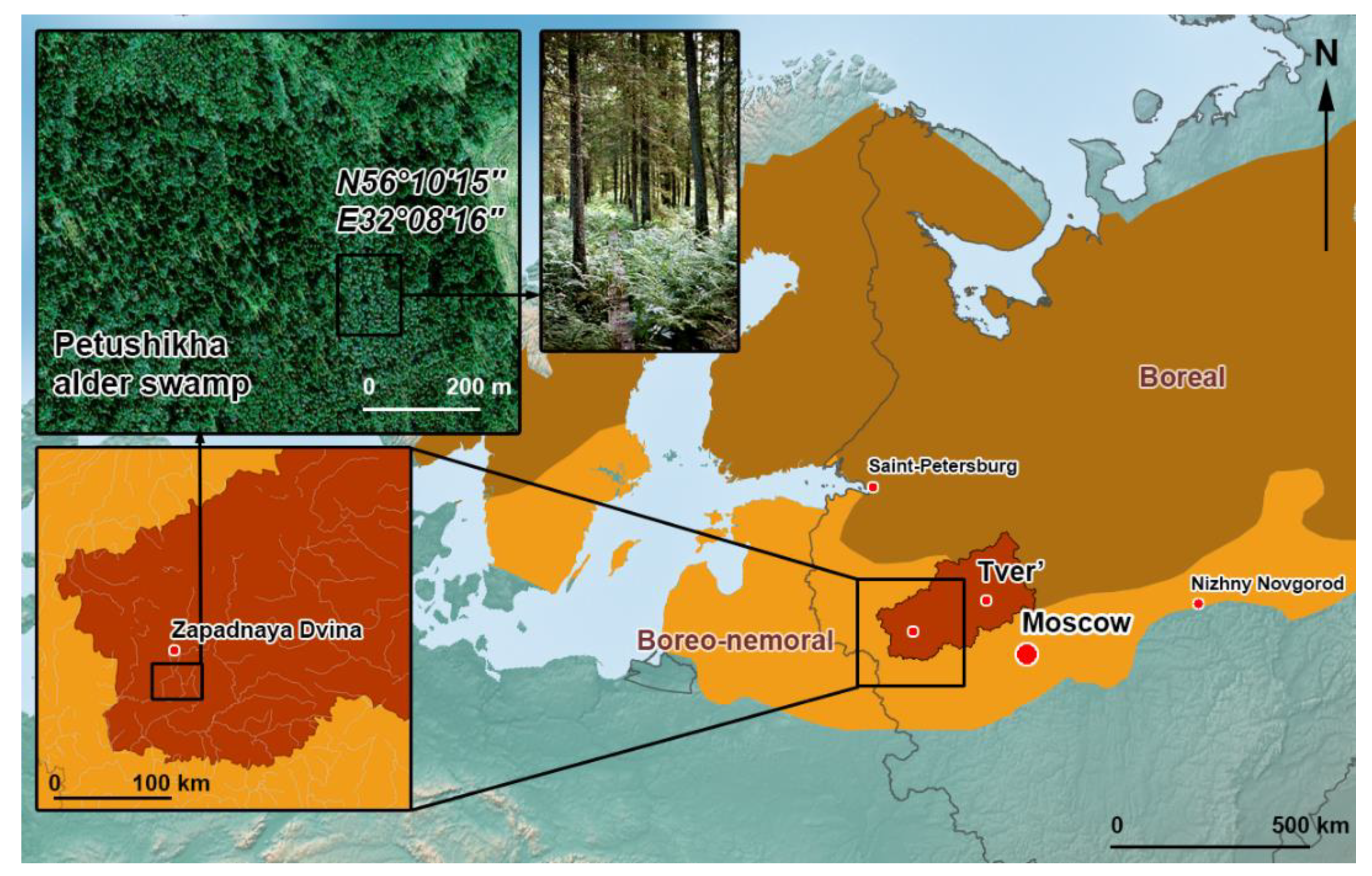
2.1. Study Location

The studies were carried out from June to October 2013–2016 on alder swamp “Petushikha” (56°10′15″ N, 32°08′16″ E) in the southern taiga zone of European Russia. The period from June to October in the southern taiga corresponds to summer (June–August) and the first half of autumn (September–October). The peatland “Petushikha” was under the influence of a powerful ecological factor throughout the history of its development—abundant water–mineral supply due to alluvial slope waters from the moraine hills adjacent to the swamp [46]. There is a swamp microlandscape closer to the periphery of the swamp, with variable flow-through moistening and abundant water-mineral supply. A virgin black alder forest with an area of 7.4 ha has formed in a flat depression at the edges of moraine hills. The water–mineral supply is comprised of atmospheric, soil–ground, and alluvial slope (of transit nature) waters; groundwater wedging out from the super-moraine horizons is observed on the surface of the swamp. The alder swamp is drained by a stream that does not have a well-defined watercourse (Figure 1).

2.2. Vegetation Cover

The composition of the stand is spruce-black alder forest with birch admixture, the average age of black alder is 99.5 years old, spruce—94.0 years old. Four layers represent the vegetation—tree, shrub, herbaceous and mossy.

The tree layer is formed by black alder (Alnus glutinosa (L.) Gaernt), European spruce (Picea abies (L.) Karst.), and partly by birch (Betula pubescens Ehrh). The shrub layer is dominated by bird cherry (Padus avium Mill), alder buckthorn (Frangula alnus Mill.), gray willow (Salix cineria L.), bay willow (S. pentandra L.), black currant (Ribus nigrum L.), and guelder rose (Viburnum opulus L.).

The background species in the herbaceous layer are lady fern (Athyrium filix femina (L.) Roth), meadowsweet (Filipendula ulmaria (L.) Maxim.), yellow loosestrife (Lysimachia vulgaris L.), bog arum (Calla palustris L.), cabbage thistle (Cirsium oleraceum L.), bittersweet nightshade (Solanum dulcamara L.), and common reed (Phragmites australis (Cav.). Background species of micro-elevations and tussocks include stone bramble (Rubus saxatilis L.), wood sorrel (Oxalis acetosella L.), and false lily of the valley (Maianthemum bifolium (L.) F.W. Schmidt). Other species are wild angelica (Angelica sylvestris L.), cowbane (Cicuta virosa L.), common nettle (Urtica dioica L.), marsh marigold (Caltha palustris L.), marsh fern (Thelipteris palustries Schott.), water horsetail (Equisetum fluviatile L.), etc.

The moss cover consists of Drepanocladus exannulatus (Bruch et al.) Warnst., D. sendtneri (Schimp. ex H.Müll.) Warnst., Callurgonella Loeske, Calliergon giganteum (Schimp.) Kindb., Climacium dendroides (Hedw.) F.Weber & D.Mohr, Brachythecium rivulare Bruch et al., Mnium rugicum Laurer. Sphagnum mosses are absent. The tree layer is mainly found on the hillocks and much less in level locations, whereas in depressions, it is absent.

2.3. Soil Cover

The soil of the alder swamp is Fibric Histosols, and the thickness of peat deposits is from 2.0 to 3.7 m. Peat has a high degree of decomposition (45–50%) and high ash content (13–24%). The high degree of peat decomposition leads to a high density from 0.16 to 0.23 g/m³. The peatland is underlain by loam. The radiocarbon (basal) age of peat is 8750 ± 70 cal. BP (IGAN-1363). The peat was dated at the Institute of Geography of the Russian Academy of Sciences, the calibrated ¹⁴ C dates (cal. BP) were calculated using the Calib 5.1 software (median) [47]. Five main elements (microsites) were distinguished in a well-expressed microrelief as follows: (1) depressions (or dead-cover hollows (DEP), reaching a depth of h = −5…−8 cm); (2) flat surface (FL; the average level of the flat surface was taken as the baseline for measuring the depths of depressions and the heights of elevations); (3) micro-elevations (EL, h = 15–20 cm); (4) tussocks of large grasses, mainly ferns (TUS, h = 15–25 cm); (5) near-stem tussocks of black alder (STUS, h = 20–35 cm). On the plot under study with an area of 0.6 ha, we carried out leveling of the soil surface in squares with a step of 2 m × 2 m. This made it possible to quantitatively assess the representativeness of various microsites. Hollows occupy 10% of the area, flat surface—35%, micro-elevations—5%, tussocks—15%, and near-stem tussocks—35%.

2.4. Field Measurements

Soil respiration (R_soil) was measured at each selected microsite using a portable Li 6400 gas analyzer (Li–COR Biosciences, Lincoln, NE, USA) equipped with a standard opaque chamber at 3–6X spatial replication. One day before the measurement, plastic cylindrical bases (collars) 15 cm high and 10 cm in diameter with a circularly sharpened bottom edge were cut into each microsite to a depth of 10 cm; the grass and moss cover were cut off at the same time. Each microsite was connected to wooden walkways to prevent the squeezing of gases out of the soil, a gas analyzer was installed on them, and a soil chamber with a flexible hose was placed on the corresponding collar. Measurements were carried out weekly from June to October in the first half of the day. Four measurement cycles were carried out (exposure time was 1–3 min) at each microsite, and the data of the last three of them were used to calculate the average CO₂ flux rate. Throughout the entire study period, the bases were installed in the same places. CO₂ flux (mgC m⁻² h⁻¹) was calculated using the following formula:

$$flux=\frac{\frac{dC}{dt}\times V\times M }{S\times Vm},$$

(1)

where C is the CO₂ concentration (ppm), t is the time (h), V is the chamber volume (m³), M is the molar mass of C (g/mol), V_m is the molar volume of CO₂ (L/mol), and S is the area of the horizontal section of the chamber (m²).

We measured the temperature of the air (T_air) and soil (T_soil) at a depth of 20 cm, as well as the level of GWL from the soil surface in parallel with the determination of CO₂ emissions. Negative GWL values indicated the water level below the soil surface, and positive values indicated above it. The air and peat temperatures were measured with sensors included among the Li–COR accessories. GWL measurements were carried out in observation wells using a hollow aluminum tube 1 cm in diameter and 150 cm in length with 1 mm marks on the outside. These wells were hollow plastic pipes 3 cm in diameter perforated along their entire length, one of the ends of which was closed with a wooden plug; all of them were fixed in mineral soil. In addition, three rain gauges were placed on the soil surface in the black alder forest. The precipitation was measured with a measuring glass with 100 divisions, each of which corresponded to 0.1 mm of precipitation.

The weighted average total soil respiration in the study area was assessed for each year (for the period from June to October) based on the data on the representativeness of various microsites. The calculation was carried out according to the formula:

$$R_{\mathrm{D}}={{\displaystyle \sum }}_{i=1}^n{D}_i\times R_i,$$

(2)

where R_D is the weighted average flux, tC ha^–1 season^–1, n is the number of types of microsites, i is the serial number of the microsite, D is the share of the area occupied by the microsite, and R is the total soil respiration at the microsite for the season (tC ha^–1 season⁻¹).

2.5. Description of R_soil Model

The R_soil model was based on an exponential dependence of CO₂ flux on the soil temperature (T_soil) [48] and a linear dependence of CO₂ flux on GWL as follows:

$$R_{soil}=\left(a\times GWL+b\right)\times R_{ref}\times Q_{10}{}^{\frac{T-T_{ref}}{10}},$$

(3)

where R_soil is the soil respiration, mgC m^–2 h^–1; $a$ and $b$ are the model parameters characterizing the dependence of flux values on GWL; GWL is the groundwater level, cm (negative values are below the soil surface, and positive values are above it); R_ref is the soil respiration at the average measured soil temperature (T_ref, °C) mgC m⁻² h⁻¹; Q₁₀ is van ’t Hoff’s coefficient; T is the soil temperature at a depth of 20 cm; and T_ref is the average soil temperature at a depth of 20 cm.

Model parameterization was carried out using all measurement data (n = 78, 172, 59, 85, and 93 for DEP, FL, EL, TUS, and STUS, respectively) without division by years. To validate the model, cross validation was used by dividing the data set into calibrating data (measurements in 2013–2014; n = 48, 114, 35, 63, and 57 for DEP, FL, EL, TUS, and STUS, respectively) and testing data (2015–2016; n = 30, 58, 24, 22, and 36). R_soil values obtained by parameterization of the model on the basis of the 2013–2014 data only were compared with the results of the 2015–2016 measurements using regression analysis (α = 0.05). We chose to use the 2013–2014 measurements as calibrating data to cover a symmetrical spectrum of moistening conditions (both high and low GWLs).

Modeling of the seasonal dynamics of R_soil was performed based on the data of two nearest meteorological stations (Vitebsk and Zapadnaya Dvina) and measured GWLs. Seasonal dynamics of air temperature (T_air′) obtained from the meteorological stations was recalculated to seasonal dynamics of T_soil′ based on the linear dependence between T_soil and T_air measured in the study area for each microsite separately for each year.

$${T_{soil}}^{’}=c\times {T_{air}}^{’}+d,$$

(4)

The coefficients of the regression equation (α = 0.05) and the statistical characteristics of the T_soil′ calculation are provided in

Table 1. Regression equation coefficients and statistical characteristics of calculation of seasonal dynamics of soil temperature T_soil′.

Year	DEP	FL	EL	TUS	STUS
	c, d, R2, n
2013	0.3, 6.9, 0.7, 20	0.4, 6.8, 0.5, 48	0.2, 9.3, 0.2, 16	0.3, 6.8, 0.4, 32	0.4, 6.7, 0.6, 24
2014	0.5, 1.4, 0.4, 28	0.8, −5.8, 0.6, 66	0.5, 2.2, 0.3, 19	0.7, −4.0, 0.6, 31	0.9, −8.7, 0.7, 33
2015	3.7, −76, 0.5, 18	0.8, −5.9, 0.5, 50	0.7, −2.7, 0.9, 12	0.8, −6.1, 0.6, 22	0.8, −6.2, 0.6, 21
2016	0.6, −2.8, 0.7, 12	0.5, −0.1, 0.8, 8	0.6, −1.1, 0.9, 12	−	0.6, −0.6, 0.9, 15

c, d are pearameters of Equation (4), R² is coefficient of determination and n is number of cases.

. All the results obtained satisfied the adequacy of the model assessed using the F-test. The GWLs measured during each field campaign were recalculated for 3 h intervals using the interp1 function with cubic polynomial dependency (Matlab 2016b, MathWorks, Natick, MA, USA). We did not make amendments for the GWLs, taking into account the position of each microsite in the relief. When using the same (within one measurement day) GWL to parameterize the model of each microsite, these differences were reflected in the coefficients a and b of the relationship between GWL and R_eco.

2.6. Data Analysis

Descriptive statistics of field measurements (average, min, max, coefficient of variation (CV), and n) was provided for measured fluxes. In the case of regression analysis, the significance of the correlation coefficient (α = 0.05) was determined by the F-test. The distribution of the obtained data for normality was checked using the Shapiro–Wilk and Kolmogorov–Smirnov test. Statistic difference between medians of fluxes was checked using the Kruskal–Wallace test (n = 487, threshold value p = 0.05; with recourse to nonparametric statistics since the fluxes values were not normally distributed), for pairwise comparison.

When parameterizing the models, their stability was checked by the stochastic method [49,50]. For this purpose, a normally distributed random error was added to the input fluxes. In this case, it was such that the CV of the input data was 15%. The models then were parameterized for 1000 repetitions, and the final coefficients of variation were calculated for the parameters (

Table 2. Results of parameterization of the soil respiration model. The dependence on soil temperature is described by parameters R_ref, Q_10, and T_ref; the dependence on groundwater level by parameters a and b. CVs are the coefficients of variation of fluxes obtained with artificially introduced CV=15% of measured fluxes.

Parameter	DEP	CV	FL	CV	EL	CV	TUS	CV	STUS	CV
a	−0.07	8	−0.04	7	−0.03	15	−0.01	38	−0.02	14
b	0.69	5	0.90	2	1.0	4	1.0	3	1.0	3
Rref	40	2	73	1	120	2	171	2	277	2
Q10	8.8	10	4.9	5	5.0	9	4.0	7	4.0	6
Tref	13.2	-	13.4	-	13.2	-	13.5	-	13.5	-

, CV) and simulated R_soil. In well-conditioned models, the CV of the parameters should not exceed the CV of the input data by more than an order of magnitude, and in the best case, it should be equal or less. A full description of the method is provided in [49,50].

3. Results

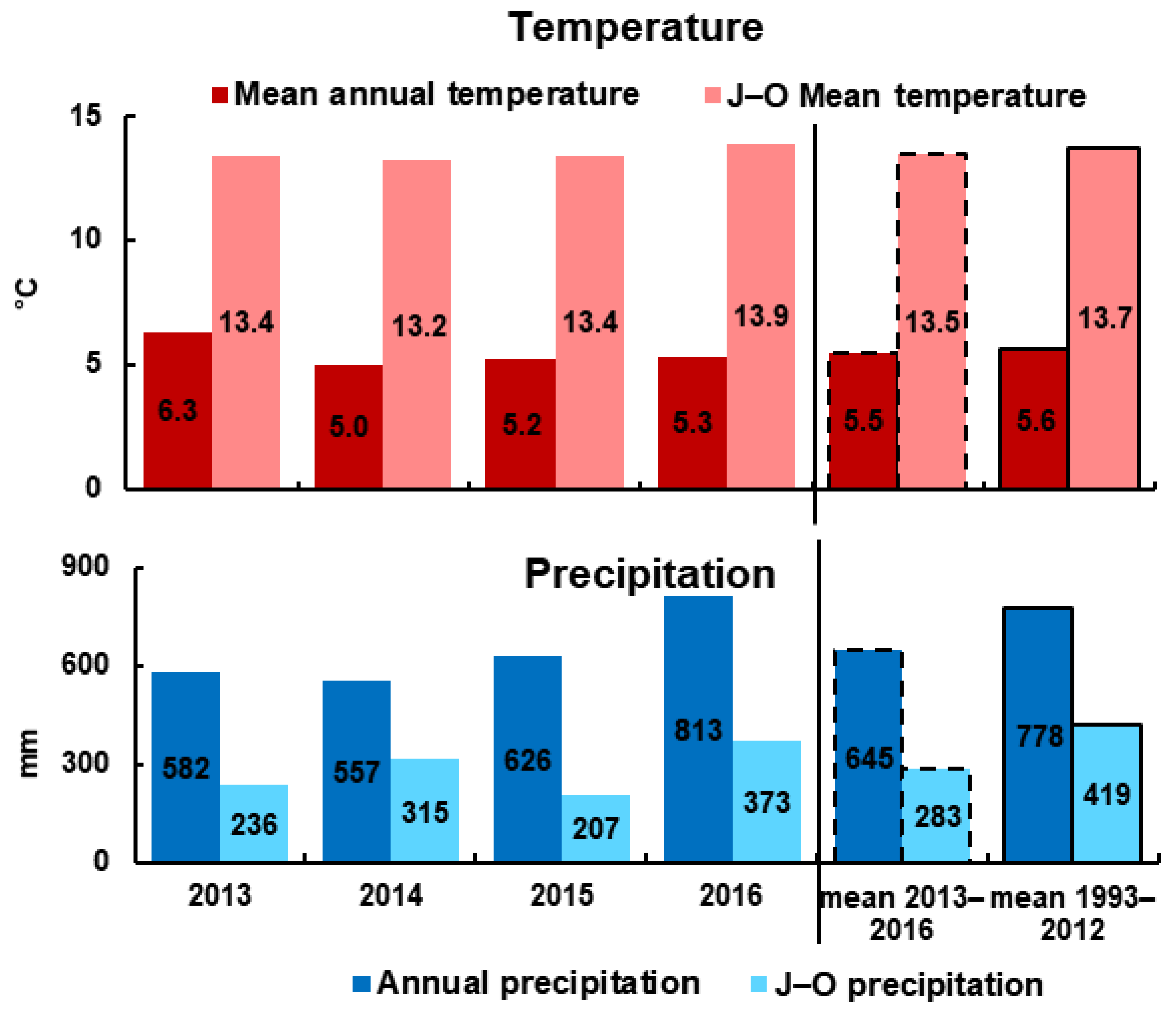
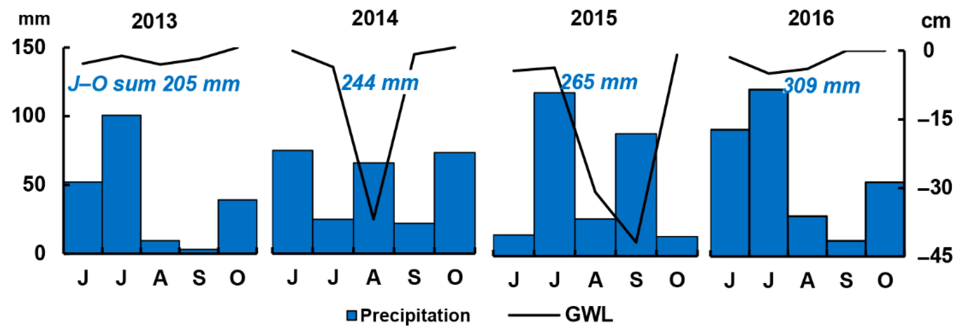
3.1. Meteorological and Environmental Conditions

The average precipitation and air temperature for the period from 2013 to 2016 and average multi-annual precipitation from 1993 to 2012, based on the results of measurements at the Zapadnaya Dvina meteorological station, are shown in Figure 2.

Average annual air temperature and precipitation registered between 1993 and 2012 at the Zapadnaya Dvina meteorological station were 5.6 °C and 778 mm, and from June to October (J–O)—13.7 °C and 419 mm. Between 2013 and 2016, both the average annual and J–O temperatures did not differ from the average multi-annual temperatures, i.e., 5.5 and 13.5 °C, respectively, while the precipitation was significantly lower, i.e., 645 and 283 mm. Average precipitation for 2013–2016 was lower than the average multi-annual by 133 mm and during the J–O period by 136 mm. This means that the J–O period was significantly drier during the measurement years, while precipitation remained constant for the rest of the year.

According to the results of precipitation measurements directly in the black alder forest, the J–O period of 2013 was the driest (205 mm of precipitation); the wettest was 2016 (309 mm). In 2014 and 2015, the J–O period had 244 and 265 mm of precipitation, respectively. On average over these 4 years, August and September were the driest in terms of precipitation (32 and 31 mm, respectively). Moreover, both in August 2014 and in August 2015, there were periods with no precipitation up to 3 weeks. In 2014, there was no precipitation from 9 July to 4 August, GWL dropped on 4 August to −34.5 cm, and on 5 August to −38 cm. In 2015, there was no precipitation from 22 July to 13 August, GWL dropped on 13 August to −31 cm, and on 1 September to −42 cm (Figure 3).

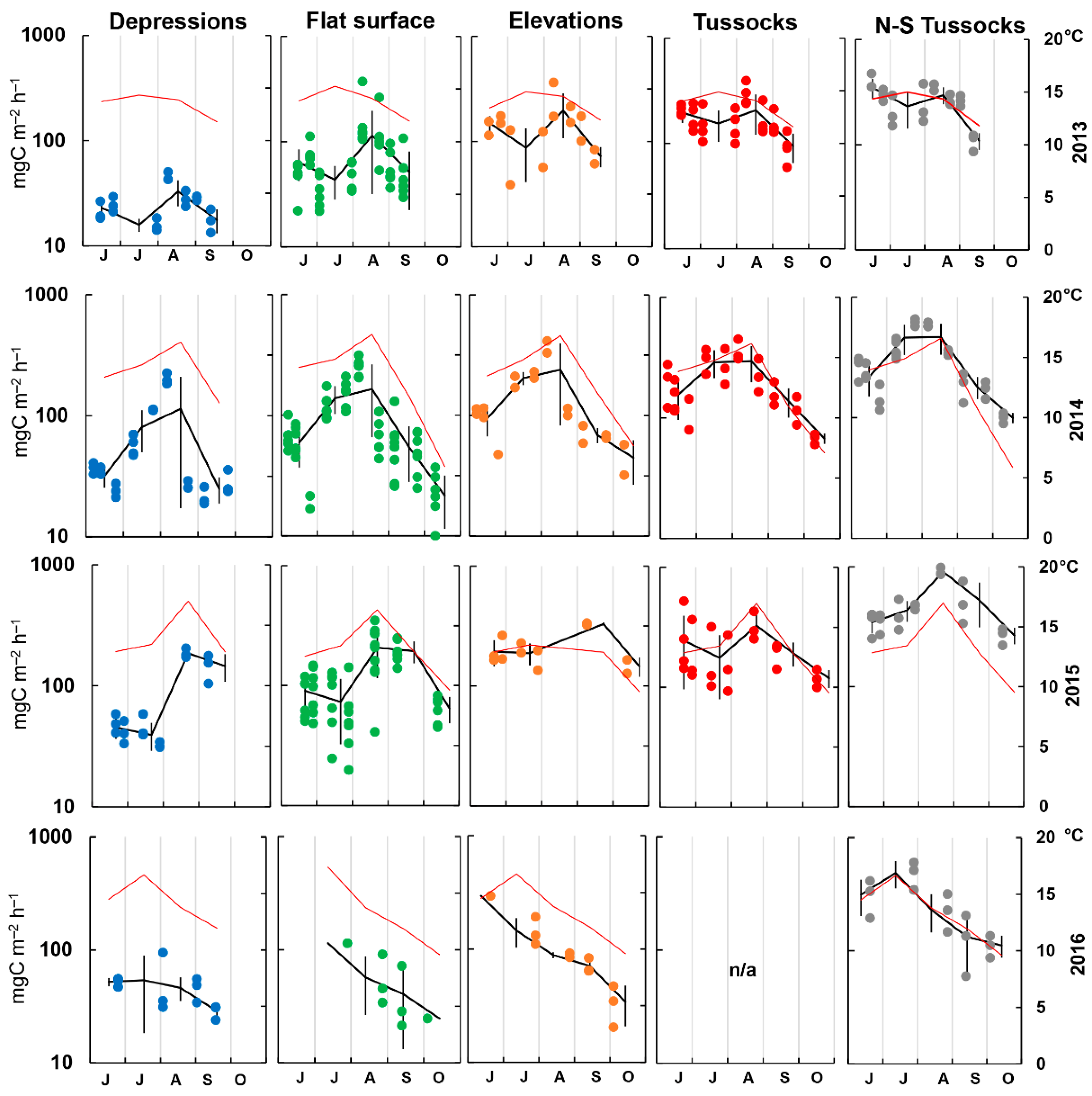
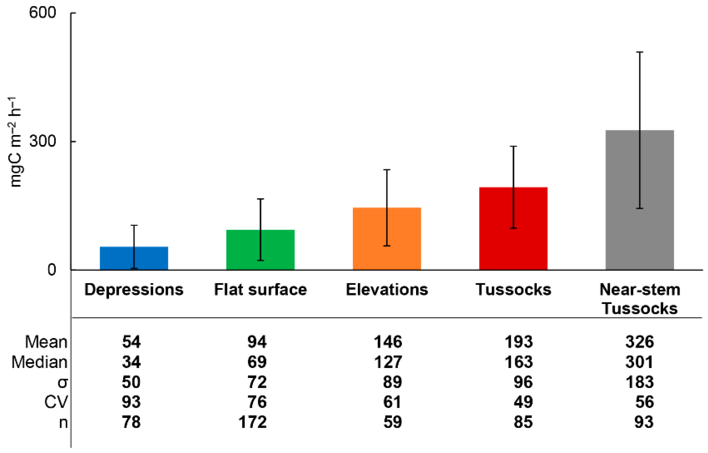
3.2. R_soil Fluxes and Environmental Parameters

Results of measurements of CO₂ fluxes (mgC m⁻² h⁻¹) at five different microsites from June to October 2013–2016 are shown in Figure 4 (note that flux values are in logarithmic coordinates). As was mentioned above, the period from June to October in the southern taiga corresponds to summer (June–August) and the first half of autumn (September–October).

The characteristic pattern of seasonal dynamics for virtually all microsites is the growth of R_soil from June to July August and a drop by September–October. In some years (2013 and 2015), there was a slight decrease in the average flux from June to July before a sharp increase in August. This may be due to the increasing of GWL as result of heavy precipitation in June (2013 and 2015) since the soil temperature continued to grow. In 2013 and 2016, R_soil peaked in June at almost all microsites, which was due to the highest (relative to the rest of the season) soil temperature during this month. In 2014, the peak of soil respiration was observed in August, and in 2015, also in August for all microsites except EL (here, the maximum of R_soil was registered in September since we were unable to perform the measurements in August for technical reasons).

Overall, the dynamics of average flux values (Figure 4, black line) weakly correlated (R² = 0.3–0.4) with changes in soil temperature; however, the correlation was somewhat stronger for microsites located higher in the relief (TUS and STUS: R² = 0.4). As expected, the main limiting factor of soil respiration at drained microsites is soil temperature, in contrast to more humid ones in which GWL is the limiting factor. In the DEP–FL–EL–TUS–STUS (from wettest to driest) microsites sequence, R² between R_soil and GWL was 0.8, 0.5, 0.4, 0.2, and 0.4, which confirms the assumption above. In general, the seasonal variability of soil respiration is extremely high: in different years, it can reach at some sites almost an order of magnitude, but more often it varies within 200–500%. Summarizing the data obtained from field measurements, we can conclude that the interannual flux variability is 150–200%, which is lower than the intraseasonal variability (200–500%). Spatial variability is the greatest (1000%) and is associated primarily with microrelief.

3.3. R_soil Flux Data Analysis

The average for all measurement periods R_soil increased in the following sequence: dead-cover hollows (DEP), flat surface (FL), elevations (EL), tussocks (TUS), and near-stem tussocks (STUS), and comprised 54, 94, 146, 193, and 326 mgC m^–2 h^–1, respectively (Figure 5). Statistic difference between medians of fluxes was checked using the Kruskal–Wallace test (n = 487, threshold value p = 0.05; with recourse to nonparametric statistics since the fluxes values were not normally distributed), for pairwise comparison. It showed p < 0.05 for all cases except EL–TUS where p = 0.11, which confirms the presence of significant differences between samples in most cases. As expected, the moistest microsites (DEP) are characterized by reducing conditions and the lowest R_soil intensity, while tussocks and elevations (TUS, EL), which are located higher in the relief and are well aerated, by a higher R_soil intensity. Microsites located on near-stem tussocks (STUS) are characterized by the maximum R_soil intensity.

It is highly likely that plants growing on the TUS and STUS microsites make a certain contribution to the increase in the flux rate. Although their aboveground parts were removed, roots and other underground parts could continue to release CO₂ through respiration or decomposition [51,52]. In addition, root exudates stimulate the intensity of microbiological (heterotrophic) soil respiration, and the availability of oxygen in numerous branched near-root pore spaces of the soil is significantly higher, regardless of whether the roots are viable or not [53,54,55,56].

At the same time, the coefficient of variation in the DEP–FL–EL–TUS–STUS sequence changed in the opposite direction: the highest relative variability of R_soil was characteristic of DEP, and the lowest of STUS (Figure 5). A significantly larger number of flux measurements performed at FL did not lead to a decrease in the coefficient of variation. Presumably, the obtained pattern can illustrate the higher flux variability due to environmental factors—soil temperature and moisture. The lower the microsite is located in the relief, and the more variable conditions are characteristic of it: the soil more often switches between overmoistened and dried up states, which is accompanied by sharper fluctuations in the temperature of its surface layer.

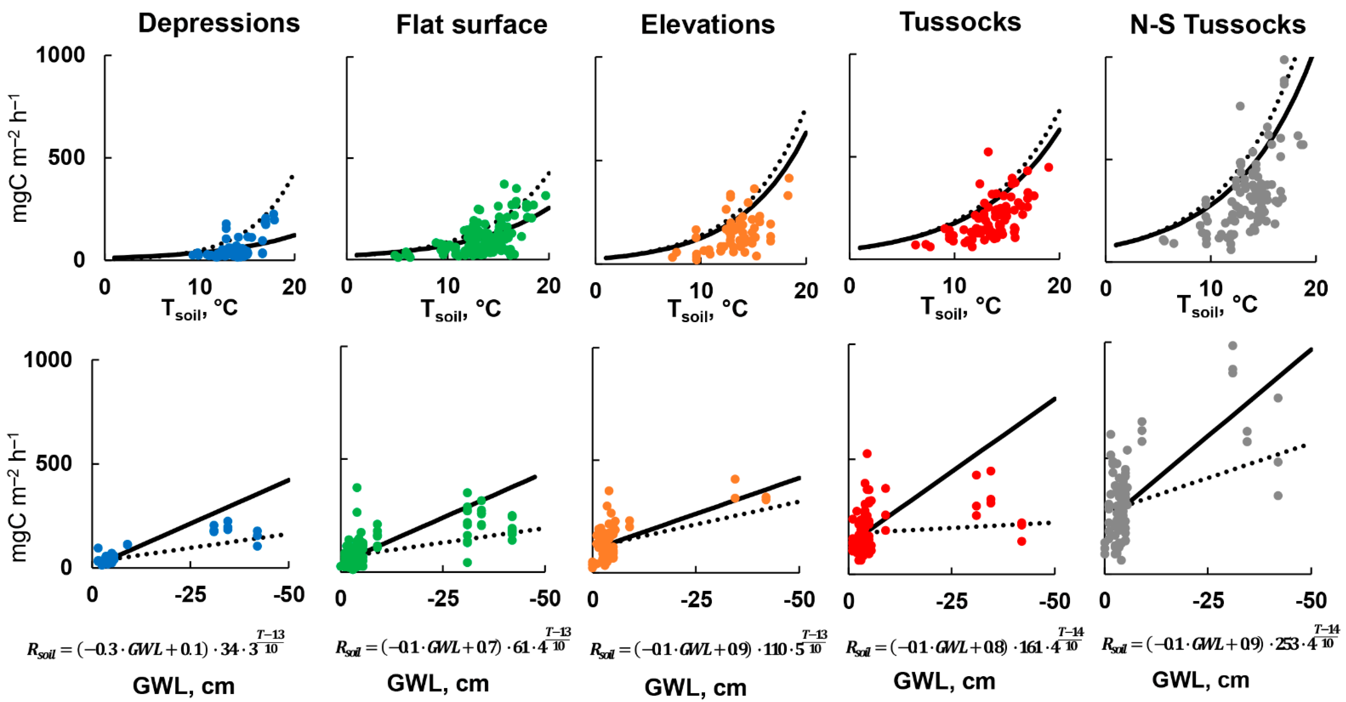
3.4. Parametrization of R_soil Model

As a result of the parameterization of the model, we obtained the values of the parameters of the dependence of soil respiration on soil temperature (R_ref, Q₁₀), GWL (a, b), and the coefficients of variation (CV) for all studied microsites (Table 2).

The most accurately at all microsites determined was to be the R_ref parameter (CV at all studied microsites did not exceed 2%, which is significantly less than the error, artificially added to the input data with CV = 15%). This was probably due to a sufficiently large number of measurements performed at each microsite. As noted above, R_ref is the soil respiration at the average measured soil temperature (T_ref), which in this case shows similar (with measured R_soil) differences between microsites: R_ref increased in the DEP–FL–EL–TUS–STUS sequence, i.e., 40, 73, 120, 171 and 277 mgC m⁻² h⁻¹, respectively. In this case, T_ref was ≈13 °C. For some microsites, the coefficient of variation of Q₁₀ turned out to be slightly higher: we were able to determine it most accurately (CV = 5%) for the microsite on a flat surface (FL). In addition to FL, the accuracy of determining the Q₁₀ parameter increased with an increase in the height of the microsite position in the relief and, accordingly, the degree of its drainage: in the DEP–EL–TUS–STUS sequence, CV of Q₁₀ was 10, 9, 7, and 6%. It can be assumed that the accuracy of determining the Q₁₀ parameter would have to depend, not on the error artificially introduced to check the stability of the model, but on the natural error caused by the variation of fluxes that is maximal at FL and minimal at STUS (Figure 4). However, in this case, we are dealing with different CVs. When considering the measurement results, this is the variability of the measured soil respiration in principle, without reference to any specific temperature or hydrological conditions, whereas in the case of the model, CV illustrates the stability of the determination of the parameters when artificial error is introduced into the input data. If the error of the determination of the parameters is significantly (by an order of magnitude) greater than the error of the input data (15% in this case), then this model is ill-conditioned [49,50]. In the latter case, one of the solutions may be a reduction in the number of model parameters, that is, its simplification, or an increase in the amount and variety of input data.

When parametrizing the model, the dependence on GWL was reflected in a somewhat worse way than that on soil temperature: CV of parameter a at the microsite TUS reached 38%, while at EL and STUS—14–15%. CV of parameter b did not exceed 5% for all microsites.

In general, the use of linear dependence between R_soil and GWL was dictated by somewhat limited information on the level of soil respiration at different moisture levels. GWL most often fluctuated in a narrow range near the soil surface over the four-year period of regular observations. We were able to register periods of sharp declines in GWL only in some months of 2014 and 2015. On the one hand, this problem can be resolved in the future by conducting more prolonged and more frequent observations, and on the other hand, by monitoring GWL at each microsite independently. Nevertheless, parameter a, which characterizes the slope of the straight line in the dependence between R_soil and GWL, increases from drier to moister microsites, which illustrates the inverse relationship between soil respiration and moisture, and a large contribution of GWL to the variability of R_soil in depressions. Taking into account that CVs of all parameters (except for a at the microsite TUS) did not exceed CVs of the input data with artificially introduced “noise,” the parameterization can be considered successful, and the model stable and well conditioned [49,50].

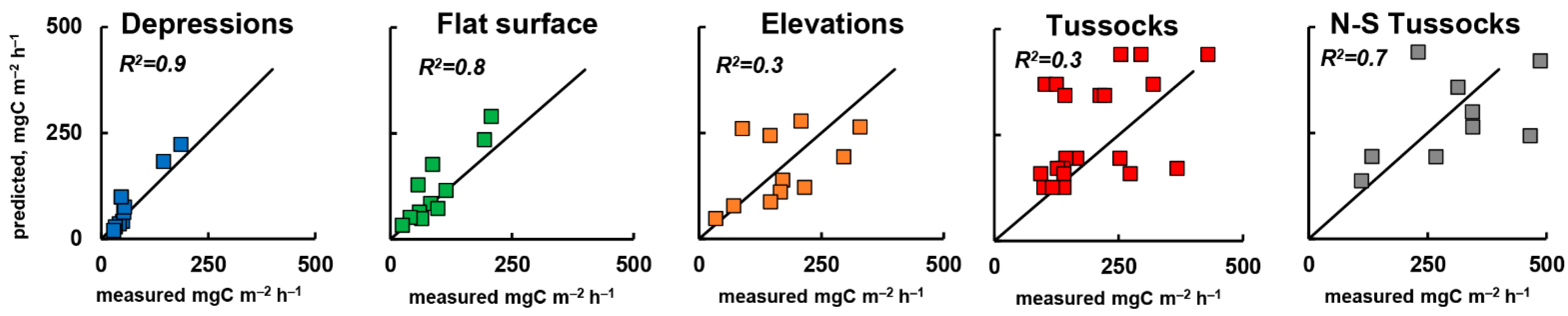
3.5. Cross Validation of R_soil Model

The results of cross validation based on the parameterization of the model using only the 2013–2014 R_soil measurements are provided in Figure 6. The abscissa shows the 2015–2016 fluxes adjusted to daily averages, and the ordinate shows the predicted (simulated) fluxes. The model predictions of R_soil work best for microsites on depressions (DEP) and slightly worse for flat surface (FL) and near-stem tussocks (STUS).

Unfortunately, the models for EL and TUS microsites require additional parameterization on a wider data set. Therefore, we decided to use the model parameterization for the entire data set (2013–2016) for all microsites when calculating the total fluxes for the season.

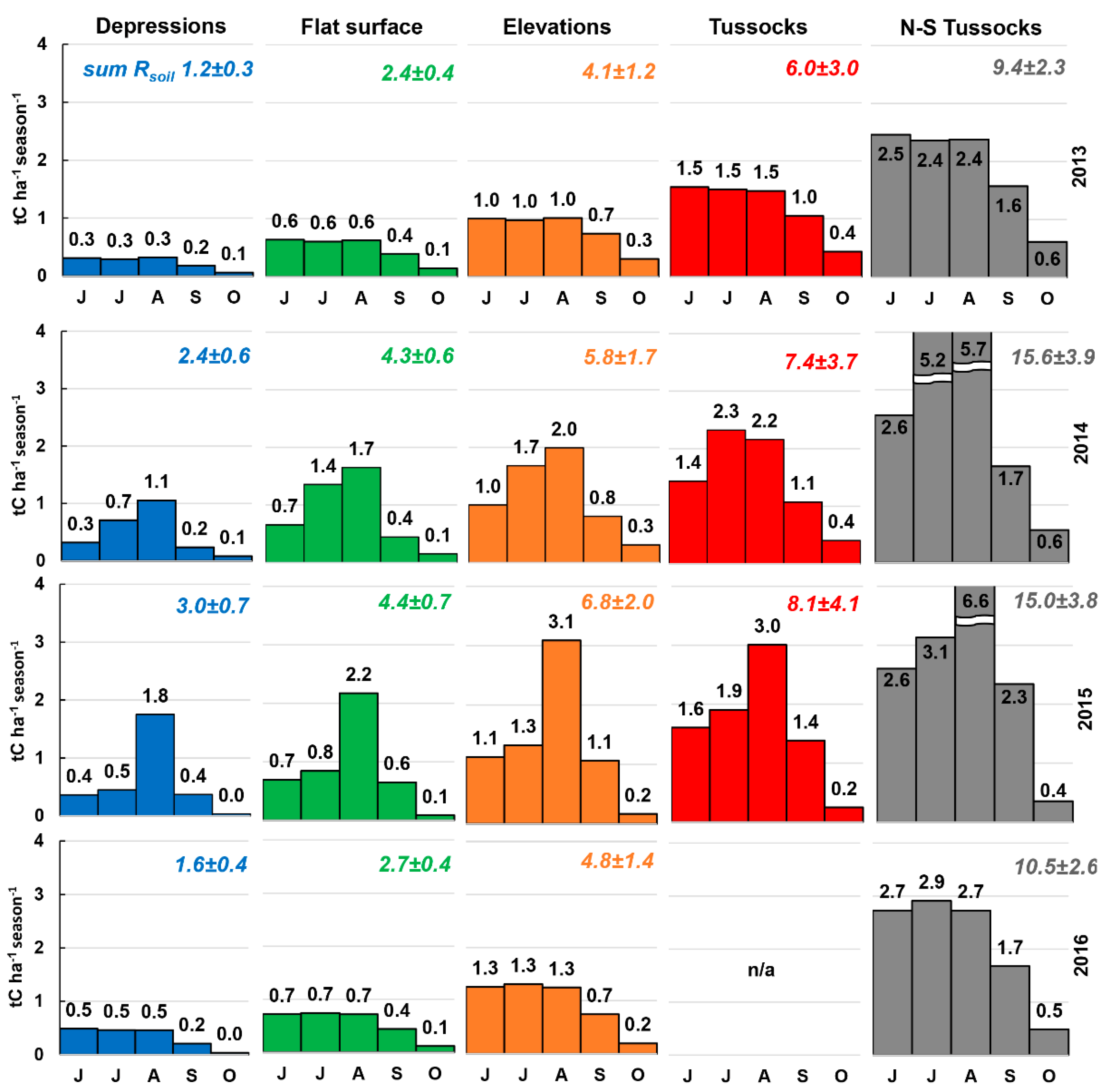
3.6. Total R_soil per Season

The results of the simulation of the seasonal dynamics of R_soil are shown in Figure 7 (note that the values are given in tC ha⁻¹). As noted in the description of the measurement results, the highest R_soil value is characteristic of the most drained microsite, STUS, and decreases with increasing moisture. In general, the results of simulation of the seasonal dynamics well correspond to the dependences observed in field conditions.

Modeling seasonal dynamics, we did not include in the calculation the estimate of the R_soil value in spring (March–May) because it is not supported by field measurements. However, considering the R_soil in June and its decrease from July to October, we could suggest that sum of spring R_soil can be noticeable. Probably the increasing of soil respiration begins immediately after the snow melts, in March–April. It is necessary to measure R_soil during these periods in the future as well; this will make it possible to parameterize the model at conditions atypical for the summer months, with high moisture content and low soil temperature.

The most contrasting seasonal dynamics of R_soil was observed in 2014 and 2015, which were characterized by high GWL variability and abrupt drying up of the surface soil layer. These abrupt fluctuations in moisture had the greatest impact on microsites in depressions. In 2015, the total R_soil in August at less drained microsites (DEP, FL) differed by 3–4 times from July and September, and at more drained ones, by 2–3 times. The magnitude of the variability in soil respiration due to temperature changes can be assessed from the results of simulation for 2016 when the GWL was relatively stable but T_soil was equally (to 2014 and 2015) variable during the season. It is highly likely that during 4 years of observations, the GWL (in particular, during rapid droughts) had a more significant effect on soil respiration than the temperature of the soil.

As a result of calculating the weighted average soil respiration on the territory of the studied black alder forest, considering the representativeness of various microsites, we established that in 2013–2016, R_soil comprised 5.4, 8.6, 8.7, and 5.0 tC ha⁻¹ season⁻¹, respectively. The calculation did not use the results of the simulation of fluxes for May since no direct measurements of R_soil were carried out this month.

4. Discussion

4.1. R_soil Fluxes and Their Seasonal Dynamics

Even in relatively distant (in terms of their ecological characteristics and geographic location) forested swamps of temperate, subtropical, and tropical regions, similar values of soil respiration are observed. For example, for the tidal swamp in Savannah National Wildlife Refuge (NWR) along the border of South Carolina and Georgia, USA, the measured soil emission of CO₂ comprised 29–59 mgC m⁻² h⁻¹, depending on the degree of moisture [57]. This is in good agreement with the results of measurements at the DEP microsite (54 mgC m⁻² h⁻¹) in the black alder forest under study, if we take into account the higher average GWL characteristic of the NWR (up to 10–30 cm above the soil surface in certain periods). Similar values of soil respiration were observed in forest ecosystems with an admixture of alder in Canada (Saskatchewa)—up to 42 mgC m⁻² h⁻¹ [58]. In another province of Canada (Quebec), CO₂ fluxes from the soil surface in a black alder forest averaged 48–69 mgC m⁻² h⁻¹, which are completely identical to the results of measurements at the DEP microsite (on depressions) [28]. Similar microlandscapes in a tropical forested swamp (hollows) emitted as a result of soil respiration from 115 to 130 mgC m⁻² h⁻¹, while in tussocks, from 115 to 220 mgC m⁻² h⁻¹ [59]; similar fluxes were registered in the black alder forest under study at microsites on a flat surface (FL), elevations (EL), and tussocks (TUS), respectively. This illustrates the work of similar ecological (soil–biological, hydrological, physicochemical) drivers that determine the level of soil respiration in different natural zones (

Table 3. Literature data on the level of soil respiration in black alder forests and ecologically close ecosystems.

Ecosystem Type	Location	Rsoil, mgC m−2 h−1	Reference
Eutrophic forested fen	Russia (West Siberia)	128	[38]
Eutrophic fen		25–370	[39]
Periodically waterlogged forest		174–414	[60]
Alder swamp	Germany	100–1008	[30]
Eutrophic fen	USA	150–350	[29]
Swamp fen	Ireland	50–400	[61]
Swamp fen	USA	29–59	[57]
Forest with alder shrub	Canada	42	[58]
Alder swamp	Canada	48–69	[28]
Swamp fen	Indonesia	115–220	[59]
Forest	European Russia	62–264	[62]
		101	[62]
Alder swamp		54–326	Current study

).

An assessment of the respiration of mineral soils showed that the processes of CO₂ release by these soils are close to the soil emission from peat soils. The value of annual CO₂ fluxes from the soddy and gray forest soils of the southern taiga zone of Russia varied from 2.7 to 11.5 tC ha⁻¹ y⁻¹ depending on the type of soil, cenosis, and weather conditions [62]. The range of these values is almost identical to that of the CO₂ fluxes in the black alder forest under study from the most moistened to the most drained microsites and comprises from 1.2–3.0 to 9.4–15.6 tC ha⁻¹ season⁻¹ considering the interannual variation. Moreover, considering potential fluxes during the winter, as in other types of excessively moistened habitats, this value may turn out to be only slightly (by about 10–15%) higher [30]. The 20-year monitoring of CO₂ emissions from soils in forest ecosystems (R_soil) of the Moscow Oblast in the Prioksko–Terrasny Nature Biosphere Reserve showed that the annual emission comprises 4.4 tC ha⁻¹ y⁻¹ [63], while the main factors responsible for the level of CO₂ emission are soil temperature and precipitation. As noted in [39], the relationship between peat soil temperature, GWL, and CO₂ emission is almost always positive and closer than the relationship between CO₂ emission, air temperature, and peat soil moisture. In the black alder forest, seasonal CO₂ fluxes (from June to October) averaged over four years range from 2.0 to 12.6 tC ha⁻¹ season⁻¹. The weighted average CO₂ flux, considering the share of microlandscapes presented, is 6.9 tC ha⁻¹ season⁻¹, which is slightly higher than that from mineral soils.

Summarizing the results obtained, we can conclude that soil respiration in the studied black alder forest well reproduces the previously obtained results in ecologically close ecosystems of forest swamps on organogenic soils, as well as in eutrophic bogs. At the same time, in some cases, for example, in forest swamps on mineral soils or in forest ecosystems without permanent swamping, R_soil was found to be somewhat lower, which is probably due to the availability and level of soil C used for oxidation by soil heterotrophs.

4.2. Influence of Extra-Dry Periods on R_soil Model Parameterization

Despite their relatively short duration, the extra dry periods observed in 2014 and 2015 were characterized by an extremely abrupt drop in GWL. It is possible that the scarcity of data on R_soil values at low GWL might significantly reduce the accuracy of the model (note the location of the clouds of points in the bottom row in Figure 8).

Moreover, despite the long and regular observations carried out at all microsites over 4 years, we do not exclude the possibility that some short periods with abrupt drops in GWL were not taken into account. In order to assess the possible contribution of dry periods to the variability of the total R_soil for the season, we carried out the parameterization of the model and the simulation of the seasonal dynamics of soil respiration without taking into account the extra dry periods of 2014 and 2015.

The dependence of R_soil on soil temperature and GWL obtained with the exclusion of periods of a sharp drop in GWL is shown in Figure 8 with a bold line, whereas the initial parameterization (taking into account these periods) is shown by a dotted line. As expected, the most significant differences concerned the parameters of the model in the block describing the relationship between R_soil and GWL: for all microsites, the slope of the straight line (described by the parameter a) increased. Probably, this means a more “powerful” increase in the intensity of soil respiration with a slight decrease in GWL relative to the soil surface (which was characteristic of 2013 and 2016) and the persistence of this effect with further decrease in GWL. We assume that this relationship should be nonlinear for different GWLs. In other words, when the GWL reaches the level of 5–10 cm below the soil surface, this leads to a more rapid increase in the intensity of soil respiration, compared to a further decrease in GWL. However, we must pay attention that within the framework of this model, the dependences of fluxes on GWL and T_soil were not analyzed separately. For a rigorous assessment of each factor, it is necessary to normalize the variables to eliminate the influence of the confounding effect. The deviation from the linearity of the dependence under consideration probably very roughly illustrates the difference between R_soil and GWL upon parameterization with and without extra dry periods. In general, the linear dependences used to describe natural processes are correct only in the first approximation and (or) within a certain interval of the parameters in question [64]. However, when designing a model, it is more important to preserve the stability of the model and to avoid its overcomplication, which can potentially lead to errors in simulated values that can reach several orders of magnitude. At the same time, simple linear dependences illustrate the general trend of changes and exclude catastrophic errors.

Some changes concerned a block of the model that describes the dependence of soil respiration on temperature. To the greatest extent, this relates to the Q₁₀ parameter for depressions (DEP)—here it changed more than twofold. When excluding the extra dry periods, we also excluded large R_soil values, which are extremely uncharacteristic of these microsites. Just as in the case of the GWL, we also cannot exclude the influence of the confounding effect on the variables, which requires further improvement of the model. However, we suppose that the result of the Q₁₀ parameterization without taking into account extra dry periods is more reliable here, and its exaggeration is an artifact of low R_soil in depressions relative to the measurement error. In other words, the fluxes at this microsite are so insignificant relative to the measurement error that they “mask” the temperature response up to a certain threshold value of soil temperature, after which there is a sharp “seeming” intensive growth of R_soil; accordingly, the value of Q₁₀ = 8.8 (Table 2).

The parameters of the model based on measurement data without considering extra dry periods are presented in

Table 4. Results of parameterization of the soil respiration model without taking into account extra dry periods. Parameters that changed most significantly (twofold or more) are underlined.

Parameter	DEP	CV	FL	CV	EL	CV	TUS	CV	STUS	CV
a	−0.25	11	−0.13	9	−0.06	26	−0.08	17	−0.06	24
b	0.11	95	0.66	7	0.94	7	0.80	7	0.88	6
Rref	34	2	61	1	110	2	161	2	253	2
Q10	3.3	12	3.6	6	5.1	10	3.6	8	3.8	7
Tref	13.2	−	13.4	−	13.2	−	13.5	−	13.5	−

. Those parameters that changed most significantly (twofold or more) are underlined. Note that the coefficient of variation of some parameters (for example, a for the TUS microsite) significantly decreased (that is, the accuracy of its determination increased), while CVs of other parameters (for example, b for the DEP microsite), on the contrary, significantly increased.

Overall, the results of parameterization without taking into account extra dry periods do not show any qualitative differences from the parameterization carried out taking them into account: R_soil retains a direct dependence on the soil temperature, and an inverse one on GWL. The values of the parameters R_ref and T_ref changed by no more than 17%, which in general may be due to the error artificially introduced at the stage of verification of the stability of the simulation.

4.3. Influence of Extra Dry Periods on Seasonal R_soil

The results of the simulation of the total R_soil for the season without taking into account extra dry periods are given in

Table 5. The total R_soil for the season calculated without considering extra dry periods (tC ha⁻¹ season⁻¹). The “diff” row shows its difference (in %) from the seasonal R_soil calculated taking into account the periods of decreases in GWL.

Year		DEP	σ	FL	σ	EL	σ	TUS	σ	STUS	σ
2013	Rsoil	0.7	0.9	1.9	0.4	3.8	1.7	5.2	1.8	8.5	3.3
	diff., %	−39		−20		−5		−14		−9
2014	Rsoil	1.7	2.0	3.4	0.8	5.0	2.3	7.6	2.6	13.3	5.2
	diff., %	−31		−21		−13		+3		−15
2015	Rsoil	1.0	1.1	2.6	0.6	5.0	2.3	6.8	2.3	11.3	4.4
	diff., %	−68		−42		−26		−16		−25
2016	Rsoil	1.0	1.1	2.2	0.5	4.7	2.1	−	−	9.6	3.7
	diff., %	−42		−19		−2				−9
mean	Rsoil	1.4		2.5		4.6		6.5		10.7
	diff., %	−45		−25		−12		−9		−14

. Differences from the seasonal R_soil values with the inclusion of periods of sharp declines in GWL (Figure 8) are shown in %: a negative sign indicates an underestimation of the obtained value, and a positive sign indicates an overestimation. When extra dry periods were excluded, a decrease in R_soil was noted for almost all microsites. This had the greatest effect on the microsites in the depressions of the relief (DEP): here, the decrease in the simulated R_soil was on average 45% over the years. The decrease in R_soil was not as significant for other microsites, i.e., 25%, 14, 12, and 9 for FL, STUS, EL, and TUS, respectively. The trend is not so pronounced; however, it can be assumed that the higher the microsite is in the relief, the less it was influenced by the periods of the GWL decrease. Nevertheless, the considered differences are exceptionally large: exclusion of only 1–2 (that is, no more than 15% out of 7–12 field campaigns from June to October per year at each microsite, respectively) measurement periods was characterized by a sharp drop in GWL from the model parameterization process, and further calculations led to differences in the estimated seasonal R_soil of up to 45%. As may be expected, the greatest differences at all microsites are characteristic of 2015, the most contrasting in moisture conditions (the drop in GWL in 2015 was faster and stronger than in 2014). At the same time, for microsites EL, TUS, and STUS, the changes in the obtained estimates of the seasonal R_soil outside of 2015 are practically the same. At the TUS microsite, the seasonal R_soil in 2014 was even higher than that in the same year taking into account dry seasons. Presumably, this is an artifact associated with slightly larger errors in performed-here model calculations in comparison with other microsites.

It should be emphasized that only a few extra dry periods can play a key part in the formation of the seasonal R_soil. In this context, it seems especially important to conduct automatic monitoring of the GWL with a high temporal resolution in the studied areas. This illustrates the complexity and ambiguity of interpretations of results obtained using single measurements outside the framework of stationary monitoring observations since, even in this case, it is difficult to guarantee the coverage of the entire spectrum of hydrological conditions of the soil that form even during one season.

R_soil measurements carried out in the alder swamp broaden the understanding of the role of swamp forests in the regional and global CO₂ balance. In addition, accounting for CO₂ from different ecosystems is important for national reporting in various countries [65,66]. Considering that potentially swamp forests can occupy significant areas, both on the territory of European Russia and other regions, their detailed studies are required. In addition, the focus of these studies should be aimed at considering the spatiotemporal dependencies on key environmental parameters of CO₂ fluxes—soil temperature, and, in particular, GWL.

5. Conclusions

Soil respiration in the alder swamp in the southern taiga of the European part of Russia varies significantly between different microsites: from 54 ± 50 in depressions to 326 ± 183 mgC m⁻² h⁻¹ ± σ in near-stem tussocks. The interannual variability of fluxes (150–200%) is inferior to the intraseasonal variability (200–500%), which, in turn, is slightly less than the spatial one (by an order of magnitude). The most important driver of R_soil at microsites in depressions is GWL, and on elevations, it is the cumulative effect of soil temperature and GWL. The total R_soil for the season varies from 2.0 ± 0.5 in depressions to 12.6 ± 3.2 tC ha⁻¹ season⁻¹ ± σ on elevations, and a significant contribution to this estimate is made by periodically appearing extra dry periods. In the absence of precipitation for 2–3 weeks, the GWL may drop by 30–40 cm, which leads to an increase in the total R_soil for the season by 9–45% at dry and moist microsites, respectively. The weighted average CO₂ flux considering the share of the available microlandscapes is 6.9 tC ha⁻¹ season⁻¹, which is slightly higher than that from mineral soils. This value can significantly increase with an increase in the frequency of climatic anomalies that for the southern taiga zone in Russia are often manifested in a shortage of moisture supply because of current climatic changes.

References

1. Parish, F.; Sirin, A.; Charman, D.; Joosten, H.; Minayeva, T.; Silvius, M.; Stringer, L. Assessment on Peatlands, Biodiversity and Climate Change; Global Environment Centre and Wetlands International: Wageningen, The Netherlands, 2008. [Google Scholar]
2. Yu, Z.C. Northern peatland carbon stocks and dynamics: A review. Biogeosciences 2012, 9, 4071–4085. [Google Scholar] [CrossRef] [Green Version]
3. Loisel, J.; Yu, Z.; Beilman, D.W.; Camill, P.; Alm, J.; Amesbury, M.J.; Anderson, D.; Andersson, S.; Bochicchio, C.; Barber, K.; et al. A database and synthesis of northern peatland soil properties and Holocene carbon and nitrogen accumulation. Holocene 2014, 24, 1028–1042. [Google Scholar] [CrossRef]
4. Drösler, M.; Verchot, L.; Freibauer, A.; Pan, G.; Evans, C.D.; Bourbonniere, R.A.; Alm, J.P.; Page, S.; Agus, F.; Hergoualc’h, K.; et al. Chapter 2: Drained inland organic soils. In 2013 Supplement to the 2006 IPCC Guidelines for National Greenhouse Gas Inventories: Wetlands; Hiraishi, T., Krug, T., Tanabe, K., Srivastava, N., Baasansuren, J., Fukuda, M., Troxler, T.G., Eds.; Intergovernmental Panel on Climate Change: Geneva, Switzerland, 2014. [Google Scholar]
5. Joosten, H.; Sirin, A.; Couwenberg, J.; Laine, J.; Smith, P. The role of peatlands in climate regulation. In Peatland Restoration and Ecosystem Services; Cambridge University Press (CUP): Cambridge, UK, 2016; pp. 63–76. [Google Scholar]
6. Leifeld, J.; Menichetti, L. The underappreciated potential of peatlands in global climate change mitigation strategies. Nat. Commun. 2018, 9, 1–7. [Google Scholar] [CrossRef] [Green Version]
7. Jurasinski, G.; Ahmad, S.; Anadon-Rosell, A.; Berendt, J.; Beyer, F.; Bill, R.; Blume-Werry, G.; Couwenberg, J.; Günther, A.; Joosten, H.; et al. From Understanding to Sustainable Use of Peatlands: The WETSCAPES Approach. Soil Syst. 2020, 4, 14. [Google Scholar] [CrossRef] [Green Version]
8. Bubier, J.; Costello, A.; Moore, T.R.; Roulet, N.T.; Savage, K. Microtopography and methane flux in boreal peatlands, northern Ontario, Canada. Can. J. Bot. 1993, 71, 1056–1063. [Google Scholar] [CrossRef]
9. Alm, J.; Korhola, A.; Turunen, J.; Saarnio, S.; Jungner, H.; Tolonen, K.; Silvola, J. Past and future atmospheric carbon gas (CO2, CH4) exchange in boreal peatlands. Int. Peat J. 1999, 9, 127–135. [Google Scholar]
10. Godwin, C.M.; McNamara, P.J.; Markfort, C.D. Evening methane emission pulses from a boreal wetland correspond to con-vective mixing in hollows. J. Geophys. Res. Biogeosci. 2013, 118, 994–1005. [Google Scholar] [CrossRef]
11. Frolking, S.; Roulet, N.T.; Moore, T.R.; Richard, P.J.H.; Lavoie, M.; Muller, S.D. Modeling Northern Peatland Decomposition and Peat Accumulation. Ecosystems 2001, 4, 479–498. [Google Scholar] [CrossRef]
12. Kleinen, T.; Brovkin, V.; Schuldt, R.J. A dynamic model of wetland extent and peat accumulation: Results for the Holocene. Biogeosciences 2012, 9, 235–248. [Google Scholar] [CrossRef] [Green Version]
13. Zhang, L.; Gałka, M.; Kumar, A.; Liu, M.; Knorr, K.-H.; Yu, Z.-G. Plant succession and geochemical indices in immature peatlands in the Changbai Mountains, northeastern region of China: Implications for climate change and peatland development. Sci. Total Environ. 2020, 773, 143776. [Google Scholar] [CrossRef]
14. Matthews, E.; Fung, I. Methane emission from natural wetlands: Global distribution, area, and environmental characteristics of sources. Glob. Biogeochem. Cycles 1987, 1, 61–86. [Google Scholar] [CrossRef]
15. Panikov, N.S.; Dedysh, S. Cold season CH4 and CO2 emission from boreal peat bogs (West Siberia): Winter fluxes and thaw activation dynamics. Glob. Biogeochem. Cycles 2000, 14, 1071–1080. [Google Scholar] [CrossRef]
16. Moore, P.D. The future of cool temperate bogs. Environ. Conserv. 2002, 29, 3–20. [Google Scholar] [CrossRef]
17. Vompersky, S.E.; Sirin, A.A.; Sal’nikov, A.A.; Tsyganova, O.P.; Valyaeva, N.A. Estimation of the areas of peatland and palu-dified Shallow-peat forest in Russia. Lesovedenie 2011, 5, 3–11. (In Russian) [Google Scholar]
18. Utkin, A.I.; Lindeman, G.V.; Nekrasov, V.N.; Simolin, A.V. Forest of Russia: An Encyclopedia; Great Russian Encyclopedia: Moscow, Russia, 1995; 447p. (In Russian) [Google Scholar]
19. Yakovlev, F.S. Black alder in the Kivach nature reserve and adjacent areas. Proc. Kivach State Reserve 1973, 2, 23–31. (In Russian) [Google Scholar]
20. Sirin, A.; Minayeva, T.; Yurkovskaya, T.; Kuznetsov, O.; Smagin, V.; Fedotov, Y. Russian Federation (European Part). In Mires and Peatlands of Europe: Status, Distribution, and Conservation; Joosten, H., Tanneberger, F., Moen, A., Eds.; Schweizerbart Science Publishers: Stuttgart, Germany, 2017; pp. 589–616. [Google Scholar]
21. Bikbaev, I.G.; Martynenko, V.B.; Shirokikh, P.S.; Muldashev, A.A.; Baisheva, E.Z.; Minaeva, T.Y.; Sirin, A.A. Communities of the class Alnetea Glutinosae in the southern Ural region. Proceedings of the Samara Scientific. Cent. RAS 2017, 19, 110–119. (In Russian) [Google Scholar]
22. Baginsky, V.F.; Katkov, N.N. Ecological features, structure and the forecast of changes of typological structure of black alder forests in Belarus. Eco–Potential 2013, 1, 84–92. (In Russian) [Google Scholar]
23. Grigora, I.M. Alder forest swamps of Ukrainian Polesye and their typology. Lesovedenie 1976, 5, 12–21. (In Russian) [Google Scholar]
24. Laivinsh, M.Y. Black alder forest communities (Carici elongatae Alnetum Koch. 1926) of lake islands in Latvia. Bot. J. 1985, 70, 1199–1208. (In Russian) [Google Scholar]
25. Timofeev, D.I. Biological and ecological features of black alder forests in boreal forests. Lesovedenie 1993, 1, 35–41. (In Russian) [Google Scholar]
26. Mander, Ü.; Maddison, M.; Soosaar, K.; Teemusk, A.; Kanal, A.; Uri, V.; Truu, J. The impact of a pulsing groundwater table on greenhouse gas emissions in riparian grey alder stands. Environ. Sci. Pollut. Res. 2015, 22, 2360–2371. [Google Scholar] [CrossRef]
27. Wroński, K.T. Spatial variability of CO2 fluxes from meadow and forest soils in western part of Wzniesienia Łódzkie (Łódź Hills). For. Res. Pap. 2018, 79, 45–58. [Google Scholar] [CrossRef] [Green Version]
28. Ullah, S.; Frasier, R.; Pelletier, L.; Moore, T.R. Greenhouse gas fluxes from boreal forest soils during the snow-free period in Quebec, Canada. Can. J. For. Res. 2009, 39, 666–680. [Google Scholar] [CrossRef]
29. Sulman, B.N.; Desai, A.R.; Schroeder, N.M.; Ricciuto, D.; Barr, A.; Richardson, A.D.; Flanagan, L.B.; LaFleur, P.M.; Tian, H.; Chen, G.; et al. Impact of hydrological variations on modeling of peatland CO2 fluxes: Results from the North American Carbon Program site synthesis. J. Geophys. Res. Space Phys. 2012, 117, 1. [Google Scholar] [CrossRef] [Green Version]
30. Kutsch, W.L.; Staack, A.; Wötzel, J.; Middelhoff, U.; Kappen, L. Field measurements of root respiration and total soil respira-tion in an alder forest. New Phytol. 2001, 150, 157–168. [Google Scholar] [CrossRef]
31. Vasilevich, V.I.; Shchukina, K.V. Black alder forests of the northwest of European Russia. Bot. J. 2001, 86, 15–26. (In Russian) [Google Scholar]
32. Parker, G.R.; Schneider, G. Biomass and Productivity of an Alder Swamp in Northern Michigan. Can. J. For. Res. 1975, 5, 403–409. [Google Scholar] [CrossRef]
33. Bulatov, M.I. Distribution of black alder in the Moscow region. Lesovedenie 1980, 5, 108–109. (In Russian) [Google Scholar]
34. Sarycheva, E.P. Spatial structure and species diversity of black alder forests of the Nerusso–Desnyanskiy Poleye. Bot. J. 1998, 83, 65–71. (In Russian) [Google Scholar]
35. Katunova, V.V. Edapho-Phytocenotic Characteristics of Black Alder Forests in the Middle Zone of the European Part of Russia (on the Example of the Nizhny Novgorod Region and the Republic of Mordovia), Actual Problems of Forestry in the Nizhny Novgorod Volga Region and Ways to Solve Them, Nizhny Novgorod; Nizhny Novgorod State Agricultural Academy: Nizhny Novgorod, Russia, 2005; pp. 81–88. (In Russian) [Google Scholar]
36. Šourková, M.; Frouz, J.; Šantrùčková, H. Accumulation of carbon, nitrogen and phosphorus during soil formation on alder spoil heaps after brown-coal mining, near Sokolov (Czech Republic). Geoderma 2005, 124, 203–214. [Google Scholar] [CrossRef]
37. Kutenkov, S.A. Swamp black alder forests of Karelia. Lesovedenie 2010, 1, 12–21. [Google Scholar]
38. Naumov, A.V.; Efremova, T.T.; Efremov, S.P. On the issue of carbon dioxide and methane emissions from bog soils of south-ern Vasyugane. Sib. Ekol. Zhurn. 1994, 3, 269–274. (In Russian) [Google Scholar]
39. Glagolev, M.V.; Golovatskaya, E.A.; Shnyrev, N.A. Emission of greenhouse gases at the territory of west Siberia. Sib. Ekol. Zhurn. 2007, 2, 197–210. (In Russian) [Google Scholar]
40. Glagolev, M.V.; Chistotin, M.V.; Shnyrev, N.A.; Sirin, A.A. Summer–autumn emission of carbon dioxide and methane from drained peatlands, changed during economic use and natural bogs (on the example of a site in the Tomsk region). Agrokhimiya 2008, 5, 46–58. (In Russian) [Google Scholar]
41. Naumov, A.V. Soil Respiration: Components, Ecological Functions, Geographic Patterns; Publishing House of SB RAS: Novosibirsk, Russia, 2009; 208p. (In Russian) [Google Scholar]
42. Glagolev, M.; Kleptsova, I.; Filippov, I.; Maksyutov, S.; Machida, T. Regional methane emission from West Siberia mire land-scapes. Environ. Res. Lett. 2011, 6, 045214. [Google Scholar] [CrossRef]
43. Kim, H.-S.; Maksyutov, S.; Glagolev, M.V.; Machida, T.; Patra, P.; Sudo, K.; Inoue, G. Evaluation of methane emissions from West Siberian wetlands based on inverse modeling. Environ. Res. Lett. 2011, 6, 035201. [Google Scholar] [CrossRef] [Green Version]
44. Glukhova, T.V.; Vompersky, S.E.; Kovalev, A.G. Emission of CO2 from the surface of oligotrophic bogs with due account for their microrelief in the southern taiga of European Russia. Eurasian Soil Sci. 2013, 46, 1172–1181. [Google Scholar] [CrossRef]
45. Bohn, T.J.; Melton, J.R.; Ito, A.; Kleinen, T.; Spahni, R.; Stocker, B.D.; Zhang, B.; Zhu, X.; Schroeder, R.; Glagolev, M.V.; et al. WETCHIMP-WSL: Intercomparison of wetland methane emissions models over West Siberia. Biogeosciences 2015, 12, 3321–3349. [Google Scholar] [CrossRef] [Green Version]
46. Vompersky, S.E.; Sirin, A.A.; Glukhov, A.I. Formation and Regime of Runoff during Hydroforestry; Nauka: Moscow, Russia, 1988; 168p. (In Russian) [Google Scholar]
47. Stuiver, M.; Reimer, P.J. Extended 14C database and revised CALIB radio–carbon calibration program. Radiocarbon 1993, 35, 215–230. [Google Scholar] [CrossRef] [Green Version]
48. Lloyd, J.; Taylor, J.A. On the Temperature Dependence of Soil Respiration. Funct. Ecol. 1994, 8, 315. [Google Scholar] [CrossRef]
49. Panikov, N.S.; Blagodatsky, S.A.; Blagodatskaya, J.V.; Glagolev, M.V. Determination of microbial mineralization activity in soil by modified Wright and Hobbie method. Biol. Fertil. Soils 1992, 14, 280–287. [Google Scholar] [CrossRef]
50. Glagolev, M.V.; Sabrekov, A.F. On a problems related to a concept of soil thermal diffusivity and estimation of its dependence on soil moisture. Environ. Dyn. Glob. Clim. Chang. 2019, 10, 68–85. [Google Scholar] [CrossRef]
51. Striegl, R.G.; Wickland, K.P. Effects of a clear-cut harvest on soil respiration in a jack pine-lichen woodland. Can. J. For. Res. 1998, 28, 534–539. [Google Scholar] [CrossRef]
52. Kuzyakov, Y.; Biryukova, O.; Kuznetzova, T.; Mölter, K.; Kandeler, E.; Stahr, K. Carbon partitioning in plant and soil, car-bon dioxide fluxes and enzyme activities as affected by cutting ryegrass. Biol. Fertil. Soils 2002, 35, 348–358. [Google Scholar]
53. Tanaka, K.; Hashimoto, S. Plant canopy effects on soil thermal and hydrological properties and soil respiration. Ecol. Model. 2006, 196, 32–44. [Google Scholar] [CrossRef]
54. Qian, J.H.; Doran, J.W.; Walters, D.T. Maize plant contributions to root zone available carbon and microbial transformations of nitrogen. Soil Biol. Biochem. 1997, 29, 1451–1462. [Google Scholar] [CrossRef]
55. Helal, H.M.; Sauerbeck, D.R. Influence of plant roots on C and P metabolism in soil. Plant Soil 1984, 76, 175–182. [Google Scholar] [CrossRef]
56. Helal, H.M.; Sauerbeck, D. Effect of plant roots on carbon metabolism of soil microbial biomass. J. Plant Nutr. Soil Sci. 1986, 149, 181–188. [Google Scholar] [CrossRef]
57. Krauss, K.W.; Whitbeck, J.L. Soil Greenhouse Gas Fluxes during Wetland Forest Retreat along the Lower Savannah River, Georgia (USA). Wetlands 2011, 32, 73–81. [Google Scholar] [CrossRef]
58. Kimball, J.S.; Thornton, P.E.; White, M.A.; Running, S.W. Simulating forest productivity and surface-atmosphere carbon ex-change in the BOREAS study region. Tree Physiol. 1997, 17, 589–599. [Google Scholar] [CrossRef] [Green Version]
59. Sundari, S.; Hirano, T.; Yamada, H.; Kusin, K.; Limin, S. Effect of groundwater level on soil respiration in tropical peat swamp forests. J. Agric. Meteorol. 2012, 68, 121–134. [Google Scholar] [CrossRef] [Green Version]
60. Glagolev, M.V.; Ilyasov, D.V.; Terentyeva, I.E.; Sabrekov, A.F.; Krasnov, O.A.; Maksutov, S.S. Methane and carbon dioxide fluxes in the waterlogged forests of Western Siberian southern and middle taiga subzones. Opt. Atmos. Okeana 2017, 30, 301–309. (In Russian) [Google Scholar]
61. Jovani-Sancho, A.J.; Cummins, T.; Byrne, K.A. Soil respiration partitioning in afforested temperate peatlands. Biogeochemistry 2018, 141, 1–21. [Google Scholar] [CrossRef] [Green Version]
62. Kurganova, I.; De Gerenyu, V.L.; Rozanova, L.; Sapronov, D.; Myakshina, T.; Kudeyarov, V. Annual and seasonal CO2 fluxes from Russian southern taiga soils. Tellus B Chem. Phys. Meteorol. 2003, 55, 338–344. [Google Scholar] [CrossRef]
63. Kurganova, I.N.; Lopes de Gerenyu, V.O.; Myakshina, T.N.; Sapronov, D.V.; Romashkin, I.V.; Zhmurin, V.A.; Kudeyarov, V.N. Natural and Model Assessments of Respiration of Forest Sod–Podzolic Soil in the Prioksko–Terrasny Biosphere Reserve. Lesovedenie 2019, 5, 435–448. (In Russian) [Google Scholar]
64. Kozlov, M. Environmental Research Planning: Theory and Practical Guidelines; Litres: Moscow, Russia, 2018. (In Russian) [Google Scholar]
65. IPCC. Climate Change 2007: Synthesis Report. In Contribution of Working Groups I, II and III to the Fourth Assessment Report of the Intergovernmental Panel on Climate Change; IPCC: Geneva, Switzerland, 2007; 104p. [Google Scholar]
66. Sheikh, M.A.; Kumar, M.; Todaria, N.P.; Bhat, J.A.; Kumar, A.; Pandey, R. Contribution of Cedrus deodara forests for climate mitigation along altitudinal gradient in Garhwal Himalaya, India. Mitig. Adapt. Strat. Glob. Chang. 2021, 26, 1–19. [Google Scholar] [CrossRef]
Figure 1. Location of the Petushikha alder swamp in European Russia.
Forests 12 00496 g001
Figure 2. (Top left): mean annual (for 2013, 2014, 2015, and 2016) air temperature (dark) and mean June–October (J–O) air temperature (light) for the same years; (top right): mean air temperature for four years (2013–2016—dotted line border) and for 20 years (1993–2012—line border) (dark) annually and for the J–O period of the same years (light); (bottom left): sum of precipitation (for 2013, 2014, 2015 and 2016) annually (dark) and for the J–O period of the same years (light); (bottom right): mean sum of precipitation for 4 years (2013–2016—dotted line border) and 20 years (1993–2012—line border) (dark) annually and for the J–O period of the same years (light).
Forests 12 00496 g002
Figure 3. Monthly precipitation (measured directly at the study site) and GWL (negative values correspond to the groundwater level below the soil surface) from June to October of 2013–2016. Sums of the precipitation (mm) for the J–O period are shown above the columns in the chart.
Forests 12 00496 g003
Figure 4. Measured Rsoil at five different microsites from June to October 2013–2016. The black line is the average flux values by month ± σ; the red line is the soil temperature.
Forests 12 00496 g004
Figure 5. Measured Rsoil fluxes and their basic statistics at five microsites in alder swamp. Statistic difference between medians of fluxes was checked using the Kruskal–Wallace test: p < 0.05 for all cases except elevation (EL) and tussocks (TUS) microsites where p = 0.11.
Forests 12 00496 g005
Figure 6. Cross validation of Rsoil model. X-axis—measured values and Y-axis—predicted values (mgC m–2 h–1).
Forests 12 00496 g006
Figure 7. Simulation of seasonal Rsoil fluxes. The upper right part shows the total for the season (June–October) Rsoil ± σ in tC ha−1 (the sum of σ of the parameters of the model).
Forests 12 00496 g007
Figure 8. Differences in Rsoil model parameterization, including (dotted line) and excluding (solid line) extra dry periods.
Forests 12 00496 g008