
Strategic Application of Topoclimatic Niche Models in Managing Forest Change


1
U.S. Forest Service, Rocky Mountain Region, Forest Health Protection, Gunnison, CO 81230, USA
2
Independent Researcher, 2424 D Street, Moscow, ID 83843, USA
*
Author to whom correspondence should be addressed.
†
retired.
Forests 2021, 12(12), 1780; https://0-doi-org.brum.beds.ac.uk/10.3390/f12121780
Submission received: 4 November 2021
/
Revised: 8 December 2021
/
Accepted: 10 December 2021
/
Published: 15 December 2021
(This article belongs to the Special Issue Adaptive Forest Management to Climatic Change)
Abstract
:Forest management traditionally has been based on the expectation of a steady climate. In the face of a changing climate, management requires projections of changes in the distribution of the climatic niche of the major species and strategies for applying the projections. We prepared climatic habitat models incorporating heatload as a topographic predictor for the 14 upland tree species of southwestern Colorado, USA, an area that has already seen substantial climate impacts. Models were trained with over 800,000 points of known presence and absence. Using 11 climate scenarios for the decade around 2060, we classified and mapped change for each species. Projected impacts are extensive. Except for the low-elevation woodland species, persistent habitat is rare. Most habitat is lost or threatened and is poorly compensated by emergent habitat. Three species may be locally extirpated. Nevertheless, strategies are described that can use the projections to apply management where it is likely to be most effective, to facilitate or assist migration, to favor species likely to be suited in the future, and to identify potential climate refugia.
1. Introduction
Climate change impacts are accruing throughout the ecosystems of the world. For forested lands, impacts are pronounced, from increased incidence of insects and disease [1,2,3] to advancing spring phenologies [4] and lengthening growing seasons [5]. Numerous niche analyses show overwhelmingly that the changes in climate expected across the 21st century will be accompanied by shifting limits of distribution, e.g., [6], such that extirpation would be expected over substantial portions of contemporary distributions of either single species, e.g., [7,8,9], or their associations [10,11]. Populations in decline may be lost, largely because the adaptedness of local populations develops over multiple generations but deteriorates rapidly under intense, adverse selection [12]. An inescapable conclusion, therefore, is the speed that the climate is changing will challenge the capacity of forest tree populations to adapt, e.g., [13,14,15].
While recommendations for adapting forests to climate change abound [16], rarely are they based on spatially explicit, quantitative projections of impacts to the relevant species. Among the exceptions, projections based on a bioclimate model were used to identify sites in western North America where Larix occidentalis Nutt. has a high probability of future suitability and to locate seed sources suitable for those future climates [17]. Recommendations based thereon were put into practice. Research in Mexico has shown that bioclimate models can be used to formulate site-specific recommendations for assisted migration [18] and to inform attempts to conserve overwintering habitat for the monarch butterfly [9]. In British Columbia, a projected increase in area suitable for Pseudotsuga menziesii (Mirb.) Franco was used to anticipate needs for seed collection and seedling production [11], and projected change was used to develop specific assisted migration recommendations for Populus tremuloides Michx. [19]. Similarly, projected changes in the area and distribution of forest types in the Czech Republic were used to recommend conversion of affected stands through harvest and planting [20].
Our goal is to develop climate niche models for 14 tree species forming the forests in the mountains of southwestern Colorado, USA; incorporate topographic effects of slope and aspect that are critical to model accuracy in mountainous terrain [21,22]; present impacts and their projections on 90 m grids that mesh easily with management units; and illustrate how the results can be used in selecting areas, species, and approaches for management. These models, considered together, can give managers a window into the future. Properly applied, they can indicate where certain kinds of management may be futile, and conversely, where they have the best chances of success into the future.
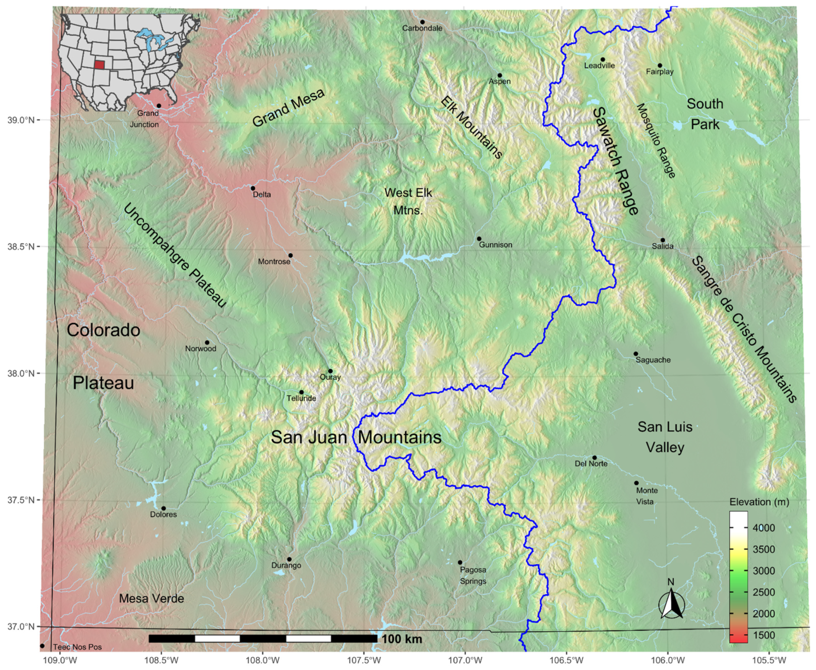
Our study area comprises the mountains and plateaus of southwest Colorado (Figure 1), a region of 94,238 km2. This region, bisected by the Continental Divide, contains headwater drainages contributing to four major river systems: Platte and Missouri to the northeast, Arkansas to the east, Rio Grande to the south, and Colorado to the southwest. Elevations range from 1300 to 4400 m, producing a diverse flora that can be assorted into seven biomes [23]: grassland and desert scrub at the lowest elevations followed ascendingly by woodlands, montane scrub, montane forest, subalpine forest, and alpine tundra.
Western Colorado and eastern Utah comprise the largest climate change hotspot in the contiguous United States, with an increase in average temperatures from 2 to 3 °C from 1895 to 2019 [24]. In our study area, mean annual temperature and mean annual maximum temperature increased 0.9 °C between our reference period, 1961–1990, and 2006–2020 (raw data from [25,26]). Both variables increased especially in spring and summer, by 1.2 °C. Precipitation did not change appreciably, but these periods do not include the record-setting turn-of-the-century drought. Considered a climate-change-type drought because it was exceptionally hot as well as dry [27], it built slowly from about 1990 and culminated in 2002. Climate projections for the area indicate that forests will be threatened by increased temperature, earlier snowmelt with longer growing seasons, increased frequency and severity of drought and fire, and increases in stress-related diseases and insects.
This changing climate has already been accompanied by substantial forest impacts in the southern Rocky Mountains. The peak of the turn-of-the-century drought (2002) was Colorado’s biggest wildfire year to that point, with one fire over 554 km2, far larger than any recorded before. Ips confusus (piñon ips) responded to the drought by killing Pinus edulis Engelm. on over 11.7 thousand km2 in southwestern USA [27]. Sudden aspen decline, which was clearly incited by the drought and followed patterns predicted by bioclimate models for the future, impacted over 4800 km2 (17% of the Populus tremuloides cover type) in Colorado [28,29]. Other bark beetles, facilitated in part by tree stress in recurring droughts, have had historically unprecedented outbreaks in the last two decades. Dendroctonus ponderosae (mountain pine beetle) killed trees on 13.7 thousand km2 in Colorado, and D. rufipennis (spruce beetle) has impacted 7.6 thousand km2 to date (Jennifer Ross, US Forest Service, personal communication). Finally, the fire year of 2020 far eclipsed 2002 in the state, with the largest total forest area burned in history and four fires ranging from 562 to 845 km2 [30,31].
Climate Niche Models and Limitations
We develop bioclimate niche models, as climate is overwhelmingly the most important natural determinant of plant distribution [32]. Paleological evidence for past changes in tree distribution correlate with changes in climate [32,33], and there is abundant evidence of changes in plant distributions with the currently changing climate [34,35,36,37,38]. The reference period for our analyses is 1961–1990, a climatic period similar to that when contemporary populations were established. Factors other than climate, such as soil and competition, also may influence distributions. The effects of soil are usually localized, and edaphic factors are generally less predictive of tree distributions than for herbs or shrubs [39]. Bioclimate niche models are based on actual distributions, where a species successfully completes its life cycle, and thus model the species’ realized niche, as limited by competition and other challenges that interact with climate.
Predicting the realized climate niche works well for climates for which the model is trained. Consequently, application to future climates is most trustworthy when future climates have reference period analogs. Analyses of climate change impacts to North American vegetation suggest that the occurrence of truly novel climates without contemporary analogs should be of little consequence in our window until, perhaps, the end of the century [10]. Yet, even though analogs may be abundant, some may occur beyond our window.
In predicting niche suitability, bioclimate models differ from species distribution models that attempt to predict the actual occurrence of the species by accounting for biotic effects and physical factors other than climate. A species may be absent from a portion of its climate niche for various reasons, such as substrate, disturbance history, competition, land use change, or migration rates that are too slow to keep up with emerging niche. Implementation of our modeled effects, therefore, relies on the expertise of land managers to integrate local factors for determining which sites within the climate niche are unlikely to be suitable.
Like any distribution model incorporating climate, climate niche models are most accurate when distributions are in equilibrium with the reference climate, and, therefore, all niche space is filled. The same contingencies apply to prediction. Consequently, our projections do not necessarily predict the future distribution of species, but rather the future distribution of currently inhabited climates.
Because of this, proper application of niche model output in future climates requires cognizance of additional factors that interact with the ecological characteristics to determine species distributions. For instance, climate change alters fire regimes and affects the behavior of insects and diseases. Fire-adapted species, therefore, may respond differently to the future climates than other species. Likewise, reproductive and dispersal traits need to be taken into account when considering colonization of new habitat. To consider such factors, ecological response models can be developed and considered in conjunction with bioclimate niche models, e.g., [40].
2. Methods
2.1. Assembling Presence–Absence Data
We used spatial vegetation files from 11 organizations (Appendix A, Figure A1) engaged in land management within the study area. These vegetation data covered 50.3% of our geographic window but accounted for nearly all of the forested lands; lands not covered by the vegetation data were mostly agricultural, steppe, or desert scrub.
The vegetation files consisted of polygons that in most cases delineated the occurrence of 14 tree species. We sampled most polygons with a 0.0025° grid, approximately 277 m for latitude and 219 m for longitude, but used a slightly finer grid (0.0023°) for polygons from the smallest management units. These sampling procedures produced 840,069 data points (see Appendix A.2 for sampling details). We assume that a species is present at a data point if the point falls within a polygon delimiting the species’ occurrence.
An additional 7280 ground plot data points from within the study area and areas peripheral to it were obtained from Forest Inventory and Analysis (FIA) (see Appendix A.3 and [41]). Treeless lands within the window but outside management unit polygons were represented by 7493 additional data points obtained from a gridded sample (Appendix A.4).
These procedures produced a dataset of 854,842 point samples (Appendix A.5), each identified by latitude, longitude, and the presence or absence of 14 species. Elevation, slope percent, and aspect (azimuth) were obtained for the gridded data from 90 m DEMs [42]. At least one of the tree species was present at ca. 81% of the data points. Populus tremuloides and Picea engelmannii Engel. were each present at ca. 35% of the data points, while 5 species were present at less than 5% (Table 1).
2.2. Climate Variables
The coordinates of each point and its elevation were submitted to a server that provides climate data [43] based on the thin plate spline climate model [44]. From the server, we retrieved for each data point climate variables derived from monthly averages for the reference period 1961–1990. Additional “transformed” variables were calculated from these derived variables.
We pared the total number of climate variables down to 12 (Table 2) for use in the climate niche modelling. These 12 have been found useful in related analyses, e.g., [22], and have a reasonably low collinearity. We also use a topographic variable, heatload [45], as a predictor (Table 2) to replace the Cartesian vectors used previously [22] for integrating the effects of slope and aspect on mountain climates. Heatload estimates potential annual direct incident radiation.
2.3. Species-Specific Niche Models
Climate niche models were built for each species using Breiman’s random forests [46], incorporating an abbreviated protocol of Huang and Boutros [47] to parameterize the algorithm. Our fine-grained datasets, in which the number of observations is far greater than the number of predictors, afford opportunities to advantageously use the “nodesize” and “sampsize” options available in the R formulation of random forests [48] to fine-tune the niche models. The “nodesize” option specifies the minimum number of observations in a terminal node, while “sampsize” allows specification of the number of observations from the minority and majority classes used for the construction of each tree.
Building the species-specific models began by randomly selecting 90% of the total observations for model development and reserving the remainder for validation. Parameterization ensued through iterations of the random forests algorithm to vet “nodesize” and “sampsize” for each model. Criteria for judging developmental models were (1) an error structure in validation analyses that was similar to the error structure in the developmental models and (2) a reasonable balance between errors of omission and commission, which, then, would yield an optimal out-of-bag error. Once satisfied that the fit of the developmental model was reflected in the verification errors, we fit a final model of 200 trees using all of the data. Fit statistics showed that errors were stable with one forest of 125–200 trees.
A stepwise elimination procedure was used to assess variable importance in each model. The stepwise process began with the 12 predictor variables (Table 2) and ended with one variable remaining, building a model at each step. In the past, we and others have used mean decrease in accuracy (MDA) to select a variable to drop at each step, but we explored the alternative statistic, mean decrease in node impurity (Gini), for variable selection. The two methods resulted in models with very similar error but with very different estimates of variable importance. In further exploration, we found that Gini could result in models incorporating randomly generated variables, while those variables were dropped when using MDA. Therefore, MDA was used at each step to quantify variable importance. The most important predictor was assumed to be the last variable remaining from the stepwise elimination process.
2.4. Mapping and Interpreting Model Output
To map reference period and future climate niches, we used 90 m grids, which, for our window, comprised ca. 14 million cells. Climate variables and heatload of each cell were estimated as described above. To make predictions, the variables for each cell were run down all trees in the forest to obtain a vote, either yes or no, as to whether the conditions in the cell were within the climatic niche of the species. Since each tree casts a vote, our analyses yielded 200 votes on the suitability of each species for each cell.
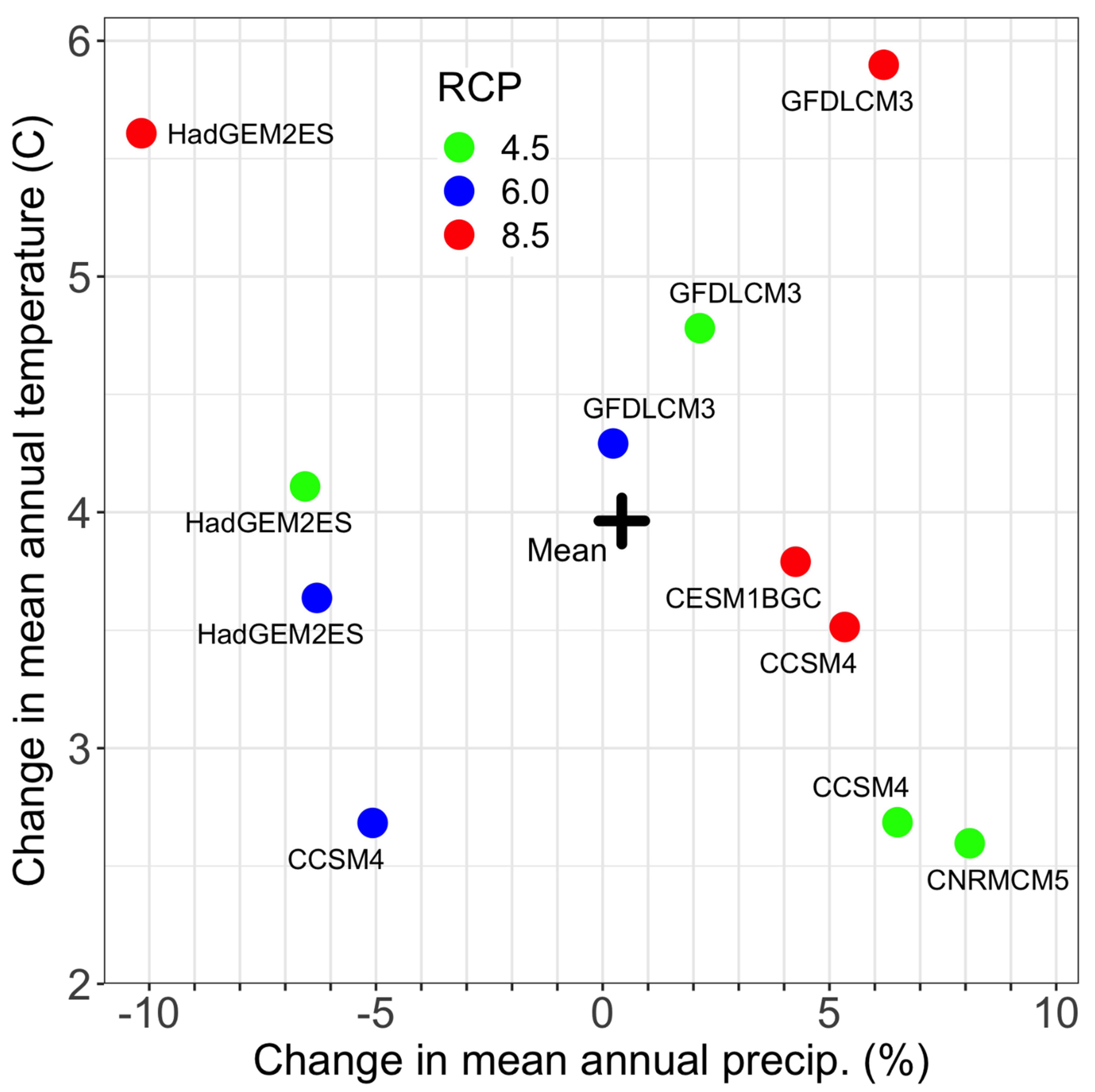
For assessing the suitability of cell conditions in future climates, we used output of 11 general circulation models (GCMs) for the decade around 2060, obtained from the climate data server, as described above for reference climate (Figure 2). For 3 GCMs (CCSM4.0 from Community Earth System, the GFDLCM3 from Geophysical Fluid Dynamics Laboratory, and HadGEM2ES from the Met Office, UK), we used climates for 3 greenhouse gas emission scenarios (RCP4.5, RCP6.0, and RCP8.5) [49]. We also used the CESM1BGC (Community Earth System Model, National Center for Atmospheric Research, RCP8.5 and CNRMCM5 (National Centre for Meteorological Research and Centre Européen de Recherche et de Formation Avancée en Calcul Scientifique, RCP4.5 output, as they, along with HadGEM2ES, RCP8.5, describe the range in variation of future climates projected for southwestern Colorado [40]. The RCP2.6 scenario was ignored because its assumptions of reduced emissions already are invalid. Heatload is a topographic vector that remains constant in time.
Votes cast for each climate were averaged in each cell to obtain the proportion of “yes” votes for future climates. We interpret niche suitability in terms of the vote proportions generated by the models and map the change in votes between the two periods according to the classification system of Table 3. In this classification, contemporary species habitat is apportioned into three classes (lost, threatened, or persistent) that project the fate of the species in future climates. An additional class, emergent, represents newly available climatic niche. The “threatened” category incorporates uncertainty similar to that of GCM projections. We refer to these classes as “habitat change classes”.
3. Results
3.1. Niche Models
In comparing errors of fit in developmental models with those in the validation dataset (Table 4), we found that out-of-bag errors could be reduced by increasing the size of the majority class, which, in our cases, were the “absences” or, in random forests nomenclature, the “nos”, and reducing the size of the minority class, the “yesses”. This, however, tended to reduce the commission errors at the expense of the omission errors, such that the lowest out-of-bag errors were accompanied by errors of omission of nearly 100%. For a niche model, such an outcome is untenable. Omission and commission errors were closest to equal when “sampsize” was set with the “yesses” equaling the “nos”, and with 100% of the “yesses” being used for developing each tree. In the case of Juniperus osteosperma, for example, each tree was built with 66,827 “yesses” (see Table 1) and the same number of “nos” (randomly sampled for each tree). In all cases, “nodesize” = 1, the default value, was superior to any other values tested.
Out-of-bag errors of our niche models ranged from 4.9% in Abies concolor (ABCO) to 15.4% in Populus tremuloides (POTR5; Table 4). Errors of commission and omission were reasonably balanced, although for A. concolor and Pinus contorta (PICO), commission errors were nearly twice those of omission.
Niche models of Picea engelmannii, A. lasiocarpa, P. tremuloides, and Pseudotsuga menziesii, four of the most abundant species (Table 1), had the largest errors of prediction. Error rates for P. engelmannii and P. tremuloides are similar to those found in previous analyses [22] dealing with a portion of our study area.
3.2. Variable Importance
The stepwise process of removing predictor variables according to importance values produced an updated out-of-bag error at each step. The change in error at each step was remarkably similar for all models. The change in error was negligible through the first seven steps, with errors increasing <0.5 percentage points. The step by which a six-variable model was reduced to five predictors on average increased errors by 1.3 points, but thereafter, errors in subsequent steps increased by 4 to 8 points. It appears, therefore, that four variables provide most of the predictive power of the model.
No single variable dominated the list of the most influential; all but two of the variables were among the top two for at least one model (Table 2). Two variables, MAPDD5 and TDIFF, appeared as the most important variable in three of the models, and heatload was among the top four variables in all models, although it was not ranked the highest for any single model. Heatload, TDIFF, and PRATIO appeared together in four-variable models for nine of the species.
To assess the contribution of heatload in accounting for micro-topographic climatic effects, we re-built the final models without including heatload among the predictors. For Pinus aristata, a denizen of high-elevation forests (Table 2), mapped comparisons (Appendix B, Figure A3) showed that heatload increased suitability on south and southwestern exposures, while reducing it on the cooler aspects. For Populus tremuloides in its broad distribution in montane and subalpine forests and for Picea engelmannii in its subalpine habitat, heatload tended to reduce suitability on southern and southwestern exposures, while adding suitability on north and northeastern exposures (Figure A4 and Figure A5). For Pinus ponderosa, a montane forest species often occurring at the woodland–forest margin, the effects of heatload at the upper limits of distribution added suitability on warm exposures, while decreasing it on northerly exposures; but at the lower limits of distribution, heatload tended to decrease suitability in broad swaths on warm exposures, while increasing suitability on the cool aspects (Figure A6).
3.3. Projected Changes
Projected impacts to the extant forests and woodlands of our window (Table 5) vary from extensive to dire. Woodland species from the lowest elevations should have a relatively secure future with high persistent habitat and with lost habitat balanced by emergent habitat. Pinus edulis (PIED) and Quercus gambelii (QUGA) would actually increase in niche area by about 30%, assuming survival where threatened. Yet, persistent woodlands account for only 20% to 50% of the current distribution, making the secure future dependent on emergent niche being filled.
For the montane and subalpine forest species, persistent and emergent habitat is generally rare; Pinus ponderosa (PIPO) has the largest proportion of persistent with 10% of the reference habitat. Nearly all existing niche is categorized as lost or threatened. Consequently, the fate of existing forests depends largely on whether the species survive in threatened habitat. Because emergent habitat is far from balancing lost habitat, forest tree species face a perilous future. The data of Table 5 portend widespread ecological disruption, the extent of which depends on whether (a) trees in the threatened class live or die and (b) species actually inhabit their emergent habitat.
Three Pinus species (P. flexilis, P. contorta, and P. aristata; PIFL2, PICO, and PIAR, respectively) may be extirpated from the area, with all reference niche lost and none emergent (except 53 cells of PIFL2 classed as threatened; Table 5). An additional species (Picea pungens) may be locally extirpated if trees in the substantial threatened areas do not survive. For these species, the models showed close agreement among climates in a lack of future suitability (votes <50%). Close inspection of votes garnered individually for each of the 11 climate scenarios showed that for PIAR, the climate would be unsuitable in 99.99% of the modeling window. At best, only two of the climates predicted suitable habitat, but only for 17 cells (0.12 km2). The PICO model predicted that all 11 climates would be unsuitable in 99.96% of the modeling window. At most, only one climate was predicted to be suitable on merely 34.5 km2. The PIFL2 model predicted that all 11 climates would be unsuitable in 99.7% of the modeling window. At most, only two climates were predicted to be suitable on 249 km2. The PIPU model predicted that all 11 climates would be unsuitable in 96.2% of the window. The highest agreement for suitability was among five climates, but only on 0.31 km2.
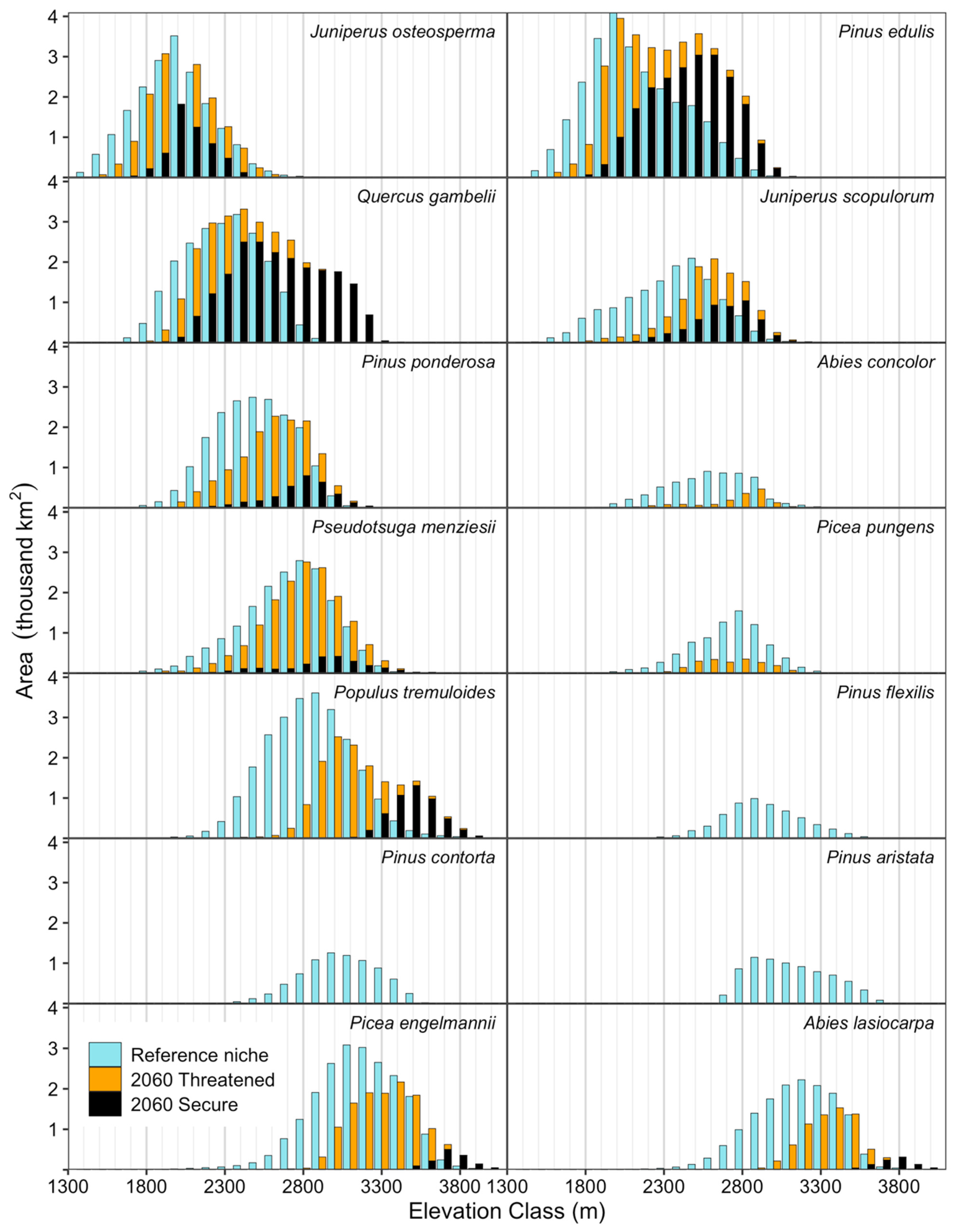
The species projected to remain within our window are expected to shift upwards in elevation while tracking a niche that may shift a few hundred meters (Table 5, Figure 3), depending on the disposition of the threatened habitat. Except for J. osteosperma, the secure portion of the future habitat distribution (persistent or emergent) occurs in the highest portion of the potential elevation distribution of the future (Figure 3).
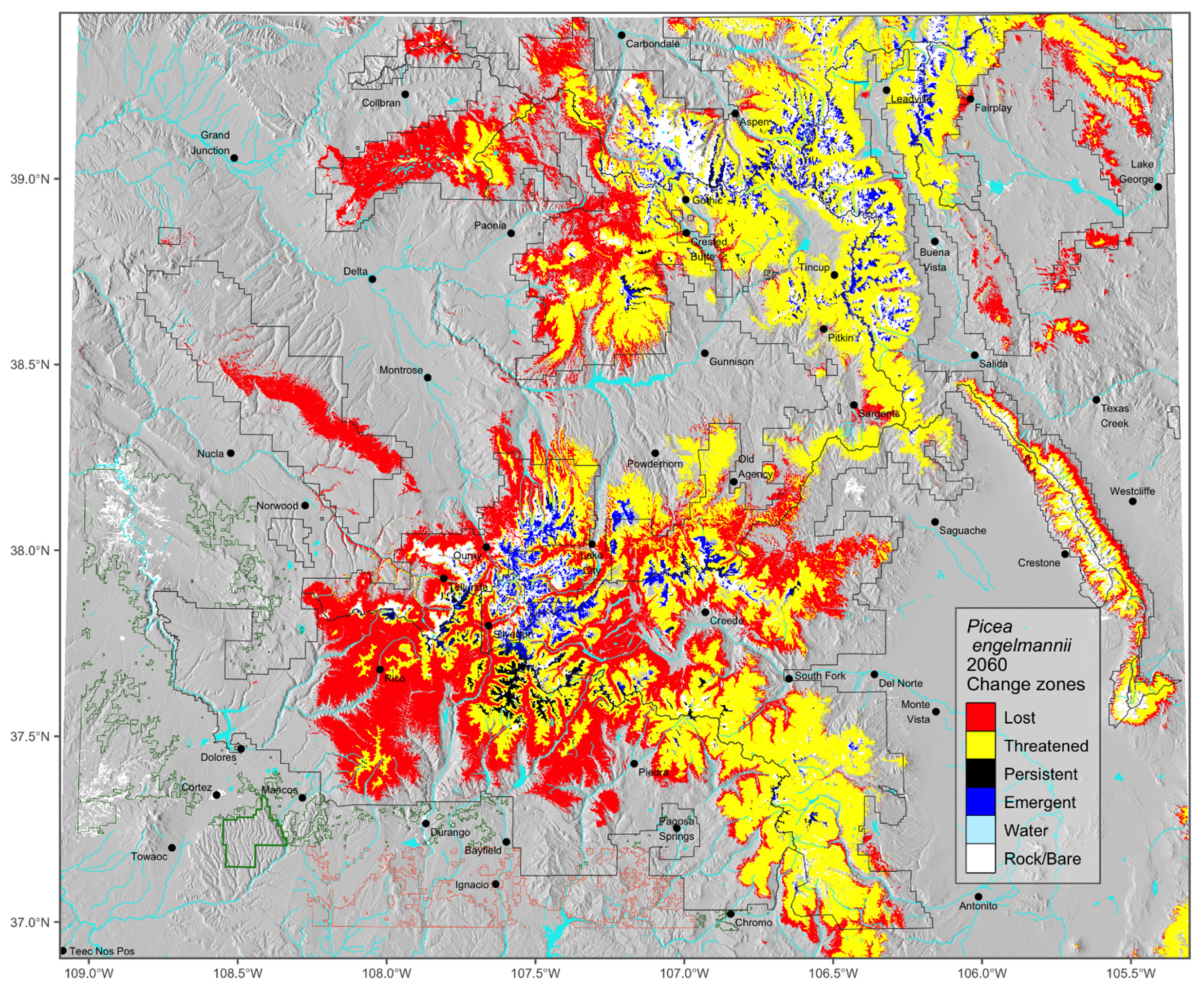
Basic to adapting forest management to climate change are the habitat change maps that use voting classifications to portend impacts to species. The change map for Picea engelmannii is Figure 4; the remainder are Figures S1–S14. The change maps illustrate the distribution of impacts detailed statistically in Table 5. The contemporary distribution of P. engelmannii of ca. 21,500 km2 is represented in Figure 4 by the sum of three categories, lost, threatened, and persistent. About 44% of this area is expected to be lost, and only 2% is confidently expected to remain P. engelmannii forest. That leaves more than half of the contemporary distribution in the threatened class. This means that the fate of the contemporary forests depends in a large part on whether the forests in the threatened class are lost or persist. While a small amount (5%) of new habitat may emerge as alpine communities are converted to forests, managers are left with the unsettling view that P. engelmannii forests will decrease in area by as much as 94% or as little as 39% of what exists today. Concomitantly, the median elevation of these forests should move upwards between 173 and 562 m.
Maps of habitat change classifications reveal several general patterns. On the Colorado Plateau in the western portion of the window, where forest habitat is intermingled with desert-scrub, change is projected to be especially negative. Most of the niche of the montane and subalpine species that occur there is projected to be lost (e.g., P. ponderosa in Figure S10, see Uncompahgre Plateau and the western part of its distribution in the San Juan Mountains). However, low-elevation woodland and montane scrub species are projected to flourish (P. edulis, J. osteosperma, Q. gambelii; Figures S3, S7 and S14). In contrast, the most favorable projections for montane and subalpine species tend to occur east of the Continental Divide (e.g., P. ponderosa, Figure S10) and at high elevations (Figure 3). The impression is that west of the Continental Divide, the climate is changing to support Great Basin communities, while east of the Divide, the climate remains supportive of the southern Rocky Mountain vegetation.
The uncertainties surrounding the threatened and emergent classes make it nearly impossible to integrate the fate of forest and woodland species into a single assessment of impacts to the forests as a whole. If all emergent niche is occupied and if all species survive in their threatened habitat, then forest and woodland niche (where at least one of the 14 species is suited) would decrease only 4% (Table 6). However, if emergent and threatened are not contributing to future niche space, woodlands and forests together should decrease 67%. If Q. gambelii is ignored as a tree species, as it is often shrub-like and considered undesirable in stands managed for timber production, those decreases in forests plus woodlands become 9% and 78%. If threatened areas do not survive, the lower timberline of woodlands may climb 300–400 m (Figure 3). The lower limit of montane forests would climb about 500 m and that of subalpine forests about 800–1000 m.
Concomitantly, the treeless portion of the study area should increase, perhaps greatly. In the reference period, treelessness accounts for 19% of our window. That portion is projected to rise to 23% at best. Yet, if threatened habitat is lost, 53% of the area could be treeless, and if, in addition, emergent habitat is not colonized, then ca. 73% of the area is projected to be treeless. If, moreover, Q. gambelii is considered to be a shrub rather than a tree, then 83% of the future window would be classified as treeless.
To be sure, our analyses concentrate on the fate of existing forests and their role in establishing a new generation. The extent that our dire forecasts can be alleviated by assisted migration from areas outside our window have not yet been systematically explored. Cursory analyses by us, however, suggest a high potential for extant populations from areas external to our window to find suitable niche among the future climates of our window. The role of assisted migration in the management of future forests of our window is a topic worthy of in-depth analysis.
4. Discussion
4.1. Uncertainty and Management
We are confident that the bioclimate models are statistically sound. By validating each model with data reserved for that purpose, errors of prediction are as low as can be expected for niche models. The models were developed for the study area with the best data and methods available. They reliably predict current distributions of realized climate niches.
Less confidence can be placed in projections of future climates that are used to predict vegetation changes. Variation in projected climates of the GCMs and scenarios is notoriously large, leading toward discussions of climate change impacts being dominated by uncertainty. Because no climate scenario is considered more likely than another, we feel the most reasonable and practical course for managers is to consider the average projected impact, which for our bioclimate models is based on the votes. Our view is to consider the variation among GCMs and emissions scenarios as a matter of time. That is, impacts tend to follow similar trajectories but occur at different times. For planning, therefore, one can assume that projected climates are reasonably accurate in their trajectory, but may be reached sooner or later than projected. Thus, the uncertainty should be no cause for inaction.
We classify niche changes between the reference period and the future as an integrated way to compare the two time periods and use thresholds to facilitate management decisions. Although averaging votes hides the underlying variation among the climate scenarios, use of the “threatened” habitat class re-introduces the variation seemingly lost in averaging and classifying vote counts.
4.2. Locally Adapted Populations (Climatypes) and Natural Selection
Our analytic approach tacitly portrays the erroneous view that species occupy a single, broad climatic niche to which all individuals are physiologically suited. Yet, most broadly distributed species are composed of climatypes that are genetically adapted to local climates (see [50]). As the climate changes, populations may become maladapted to the new conditions [14,51], even though suitable climatypes may occur elsewhere. Thus, even in habitat considered to be persistent according to the bioclimate models, the local populations may not be suited to the new climate. Obtaining new forests of adapted trees may require planting programs to assist the migration of trees to the new location of the climate to which they are suited [52]. Wherever planting is a viable option, managers have the opportunity to introduce populations from within or beyond our window to the new location of their optimal climate.
Alternatively, in persistent zones, natural selection may help the local population to adapt to the changing climate. To facilitate selection, treatments that stimulate high rates of reproduction should be encouraged. Indeed, the recent stand-replacing disturbances in the modeled area from spruce beetle and wildfire may provide a large population of seedlings and saplings that can be selected naturally as the climate changes. However, multiple generations may be needed to develop a climatype for a new climate, and climates seem to be changing faster than this process can accommodate [14,15]. For this reason alone, planting seems to be the most viable option.
4.3. Vegetation Change and Climate Analogs
A concept basic to interpreting vegetation change is that future climates will be suited for the vegetation occurring in their reference period analogs. That is, species and their climatypes will track the climate to which they are adapted, and, therefore, the realized climate niche of the future will recur in climates similar to where they occurred in the past.
Yet, seemingly counter-intuitive projections frequently occur. Since climate is the primary factor controlling niche changes in an elevational sequence, it is often assumed that species will systematically move up in elevation as a result of climate change. Indeed, our analysis suggests that the future occurrence of contemporary climatic niches will generally be at higher median elevations than reference niches. However, our projections also show that the upwards shift will not necessarily occur in such an easily predictable fashion. In fact, some altitudinal sequences disappear entirely in portions of our window.
On the west side of the Continental Divide, particularly the southwest portion of our study area, species change maps suggest that two montane species, P. ponderosa and P. menziesii, may eventually disappear, having little habitat classified as persistent or emergent (Figures S11 and S13). Yet, Populus tremuloides and subalpine species (Picea engelmannii and A. lasiocarpa) are expected to shift upwards into emergent habitat. However, east of the divide in the northeast corner of our window (Figure 5, Figure S11) P. ponderosa retains its position in the altitudinal sequence, as all of these species shift upwards. This apparent anomaly has been addressed in preliminary analyses of climate analogs that suggest to us that the P. ponderosa niche suited to extant populations west of our study area should arise in the southwest portion of our window, particularly in the San Juan Mountains, as the contemporary niche deteriorates.
For understanding seemingly illogical projections, climate analog analyses appear as a useful complement to niche projections, e.g., [53]. Climates analogous to future climates within our window undoubtedly exist today beyond the window. It is also possible that future climates could arise within our window that have no contemporary analogs beyond the window. Such occurrences are expected to render niche projections less reliable, as competitive interrelationships are known to break down in novel climates [54]. Either case could be identified readily with analog analyses.
4.4. Application to Management
4.4.1. General Application of Change Classes
The most important use of change zones may be not changing how management is done, but where it is done. Conservation can be optimized and resources used most efficiently by identifying areas with the most favorable projected habitat and managing to protect and regenerate the appropriate species there. The goal is focusing each management action where it is likely to be most effective into the future. If, however, management areas are pre-determined because of a project’s purpose and need, projections can be used to identify which species to favor during management.
A good way to address uncertainty in management is the use of “no regrets” strategies, those that are beneficial under multiple scenarios and have little or no risk of socially undesired outcomes [55]. Such actions benefit resources and values, regardless of climate-change effects. Actions discussed below generally meet those criteria.
Lost Habitat. In general, investment with the goal of improving or managing for the future of a species should be a low priority where its habitat is projected to be lost, as it has the least likelihood of long-term success. However, management may be needed for other reasons, such as reducing fire risk near communities. In that case, establishing young age classes and managing at low stocking levels may help the “lost” species persist longer. More future-suitable species should be favored or introduced where possible. For valuable species that are projected to be almost or completely lost, we can identify areas where their survival is most likely and manage those appropriately (see Refugia below).
Threatened Habitat. If other options are limited, consider treating sites within the threatened class that have the highest future votes to increase resilience to drought, diseases, and insects, especially in stands where more future-suitable species can be favored. In both lost and threatened habitat, a species may persist for many years as mature individuals if, for instance, the climate no longer favors recruitment but can sustain mature trees. This may be especially true for P. aristata and P. flexilis, which are long lived and known for withstanding extreme drought after they are well established.
Persistent Habitat. Normal management can proceed with reasonable confidence, but in our window, persistent habitat is limited and may be considered a climate refugium (see Refugia below). In general, enhancing species’ resilience is important in persistent habitat, as it may become threatened later, and the local populations may become maladapted, even if it remains persistent at the species level. Consideration can be given to increasing opportunities for regeneration, enhancing age diversity, and creating landscapes that reduce vulnerability to bark beetles and large-scale catastrophic fire.
Emergent Habitat. Facilitate migration as appropriate for the species and site. For example, some species may benefit from soil disturbance or fire on some sites for seedling establishment. Consider assisted migration (planting) as the climate changes. Emergent habitat will not be colonized quickly in many cases and will depend on proximity to and fecundity of seed sources [56]. Migration will be most successful where emergent habitat is adjacent to threatened or persistent habitat. Natural migration rates vary widely among species, but, except perhaps for light-seeded species such as aspen, natural migration is expected to be much slower than rates of habitat change, e.g., [13].
4.4.2. Management Tactics and Examples
Here, we offer examples of how the models can be used in planning management under various circumstances.
Encourage a Mix including Future-Suitable Species
When planning management activities in a predetermined project area for any reason, compare current species composition with species projected to be suitable there in the latter part of the century. Encourage any existing future-suitable species over those projected to be lost or threatened and consider planting species for the future.
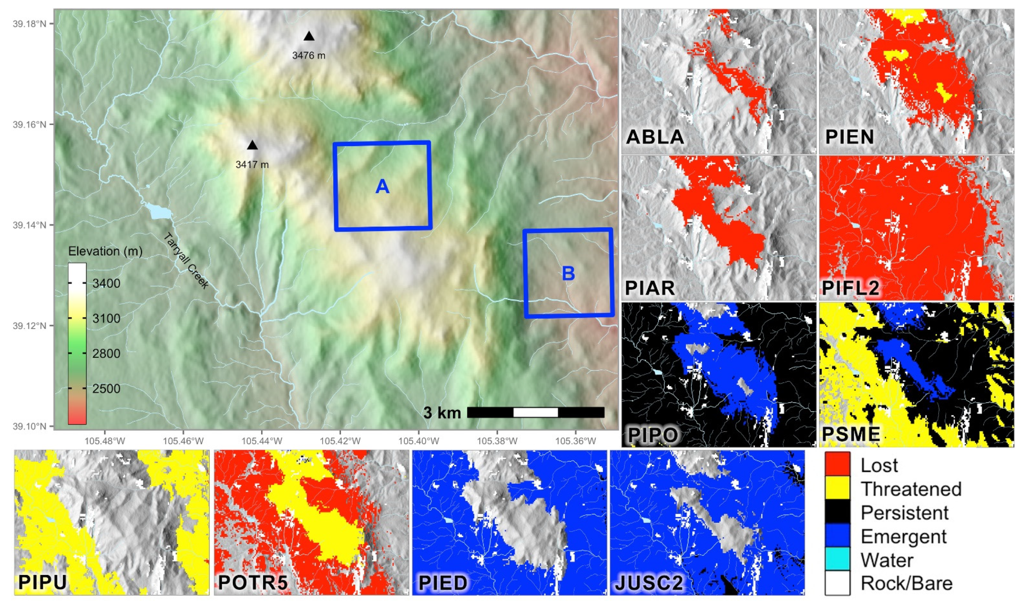
For example, project areas may be identified to fulfill a project’s purpose and needs other than climate adaptation (Figure 5). Pinus aristata and P. flexilis, which are widespread in the reference period, are expected to be completely lost. In area A (Figure 5), at high elevation, spruce–fir forests recede, becoming threatened at best, while P. ponderosa and Pseudotsuga menziesii emerge from below. Populus tremuloides is threatened in its reference niche, but emergent around the peaks. Based on these change projections, harvesting or otherwise disturbing patches of spruce–fir near P. ponderosa and P. menziesii may create opportunities for migration into their emergent niches. Dead and dying Picea engelmannii stands farther from P. ponderosa seed sources could be planted with appropriate P. ponderosa seed sources. Where P. menziesii is persistent, it is desirable to encourage regeneration and maintain fire-resilient stand structure. Where aspen is threatened, aggressive coppicing is likely to increase drought resilience [29], but emergent or persistent conifers should be retained.
In area B, at lower elevation, P. ponderosa is well established and persistent throughout. Picea pungens is threatened, and Pseudotsuga menziesii is threatened to persistent. Piñon–juniper woodlands (Pinus edulis–Juniperus sp.) are emergent. To optimize survival, P. ponderosa can be managed for age diversity, resilience to fire and bark beetles, and reduction of dwarf mistletoe. Where P. menziesii is persistent, it can be managed similarly. Piñon–juniper should be retained and protected if it migrates into its emergent areas. Because migration of woodland species is notoriously slow, planting may be necessary for timely site occupancy.
Use Projected Change and Votes as Criteria to Choose Locations for Management
When planning a project that has flexibility in choosing areas to manage, criteria often include stand conditions, road access, slope, and management emphasis. Projections can be added to those criteria to choose areas where management has the greatest chances of success.
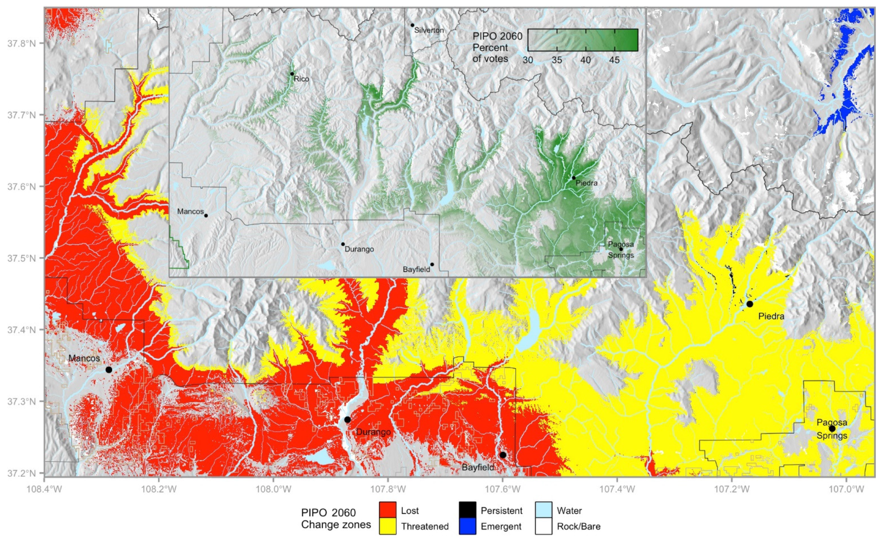
For example, in the San Juan National Forest (Figure 6), P. ponderosa in lost habitat may be given lower priority, unless there are other important criteria for site selection. Work there may include salvage and favoring species projected to be more suited to the site in the future. Persistent areas near Piedra Campground (Figure 6) could be prioritized to enhance stand resilience to drought, fire, and bark beetles. Because persistent habitat is so limited, the best quality threatened habitat can be selected based on the highest future votes (Figure 6, inset), focusing on increasing stand resilience and favoring other, future-suitable species.
Identify Potential Climate Refugia for Special Management
Species that are considered valuable ecologically, culturally, or economically may be in jeopardy if the local habitat is projected to be all lost or all lost and threatened. Models can be used to identify sites with the most favorable habitat, which can then be managed to minimize the chances of local extirpation.
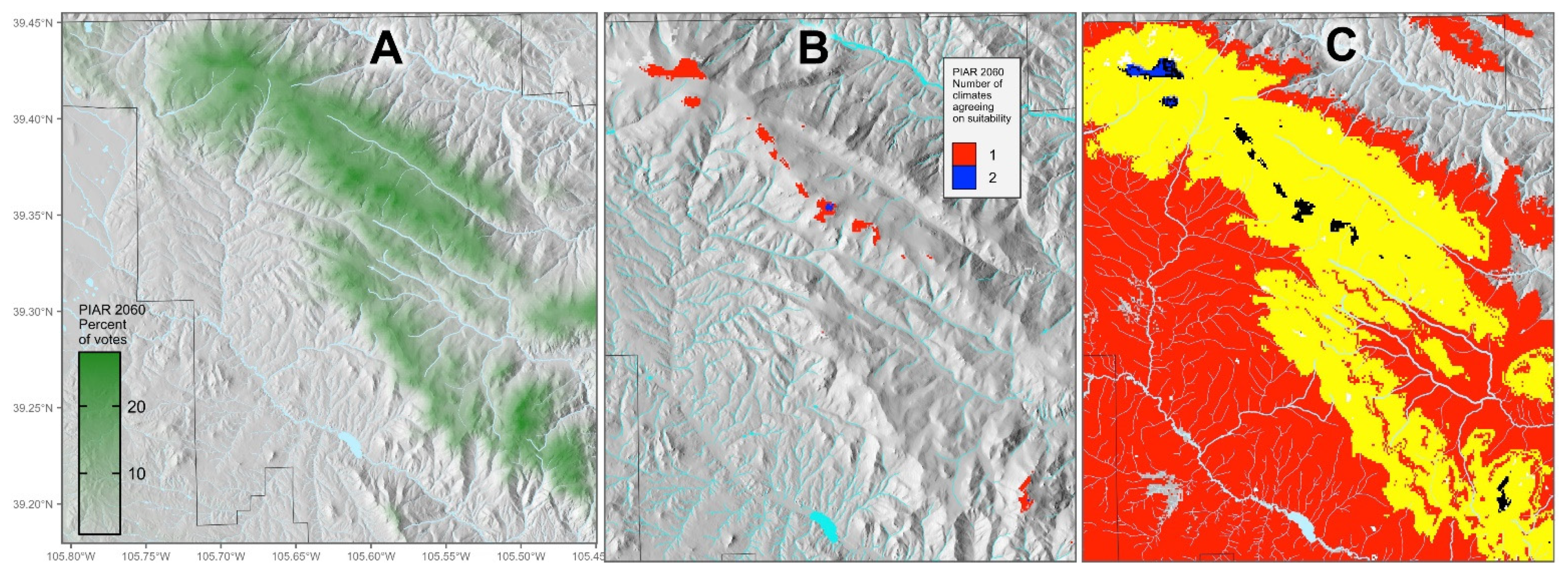
For example, P. aristata (bristlecone pine) is a valued cultural resource as well as being important to wildlife, but projections show its habitat to be lost with none emergent. By using continuous votes rather than the change classes, areas most likely to approach persistence can be identified (Figure 7A). Then, by examining the projections based on each of the 11 GCM climate scenarios we use, we find two climates that result in suitable habitat in pockets at high elevation (Figure 7B), the most favorable being CNRMCM5_rcp45. A change map based on that climate alone suggests limited amounts of persistent habitat along with a broad belt of threatened habitat should accompany the lost habitat at lower elevations (Figure 7C). The potential persistent habitat, thus, identifies the most likely climate refugium in the study area. Consideration can then be given to management to increase regeneration opportunities, reduce potential for stand-destroying fire, and increase resilience to mountain pine beetle.
Facilitate Migration
Consider strategies to enhance natural colonization of emergent habitat. In many cases, this is not feasible, and assisted migration (planting) should be considered.
For example, the upper Uncompahgre Plateau is projected to lose most habitat for species that are currently there, but Pinus edulis (piñon), which is currently on the lower shoulders of the Plateau, has emergent habitat there. Various corvid species, jays and nutcrackers, are important in long-distance seed dispersal of piñon. Treatments can be considered to improve habitat for these birds, especially at and above the current upper elevation of piñon. Implementing these tactics may facilitate natural migration of piñon toward the mesa top.
Populus tremuloides (aspen) has very light, wind-blown seed, and many studies have shown that seedling establishment is much more common than previously believed. Where aspen has emergent habitat, disturbance, especially fire, will enhance the likelihood of seedling establishment. Aspen stands upwind of emergent habitat can be evaluated readily to identify female clones. In those stands that have been heavily invaded by conifers, coppice-cutting would re-establish pure female aspen, ensuring a long-term supply of abundant seed.
4.4.3. Management Restrictions
Applying tactics based on model results can be stymied by current management restrictions. For instance, the only extensive area of persistent Picea–Abies forest projected for the future by our models is on the central San Juan National Forest in the Weminuche Wilderness, the largest wilderness area in Colorado (Figure S2 and Figure 4). Roads and machinery are currently prohibited there, making active conservation of this climate refugium difficult to impossible. Existing mining claims, grazing allotments, and water rights may also interfere with implementation of worthy programs.
Supplementary Materials
Figures S1–S14 are available online at https://0-www-mdpi-com.brum.beds.ac.uk/article/10.3390/f12121780/s1: Distribution of habitat change classes (i.e., change zones) based on the categories defined in Table 3 and mapped at 90-m resolution. Change maps for Abies concolor, Abies lasiocarpa, Juniperus osteosperma, Juniperus scopulorum, Picea engelmannii, Picea pungens, Pinus aristata, Pinus contorta, Pinus edulis, Pinus flexilis, Pinus ponderosa, Populus tremuloides, Pseudotsuga menziesii, and Quercus gambelii.
Author Contributions
Conceptualization, methodology, and writing, J.J.W. and G.E.R.; data preparation, J.J.W.; model development and validation, G.E.R.; visualization, J.J.W.; formal analysis, G.E.R. and J.J.W. All authors have read and agreed to the published version of the manuscript.
Funding
Partial funding at an early stage was provided by Western Wildland Environmental Threat Assessment Center, US Forest Service.
Data Availability Statement
Rasters produced in this study, including distributions of model votes for the reference period, mean votes for the decade around 2060, and 2060 change classes, are openly available in the Environmental Data Initiative at https://0-doi-org.brum.beds.ac.uk/10.6073/pasta/b170d82450ca0da224fdd2bc0e23d776. (accessed on 4 November 2021) Future vote rasters for individual climates will be provided on request.
Acknowledgments
Carole Howe provided assistance, files, and information on numerous occasions in support of assembling presence–absence data. Nicholas Crookston assisted with programming strategies, code in R, and made spline climate data publicly available. Renée Rondeau and Michelle Fink of Colorado Natural Heritage Program prepared one of the rasters we used and collaborated in related work that stimulated our thinking. Marcie Bidwell of the Mountain Studies Institute organized a workshop in which preliminary results were shared with managers. Suzanne Marchetti processed many of the shapefiles used in development of presence–absence data and mapping and contributed ideas to early stages of the project. Helpful pre-submission reviews were kindly provided by Todd Gardiner, Paul Hennon, and Renée Rondeau.
Conflicts of Interest
The authors declare no conflict of interest. The funder had no role in the design of the study; in the collection, analyses, or interpretation of data; in the writing of the manuscript, or in the decision to publish the results.
Appendix A. Assembling a Presence–Absence Dataset
Appendix A.1. Vegetation Data
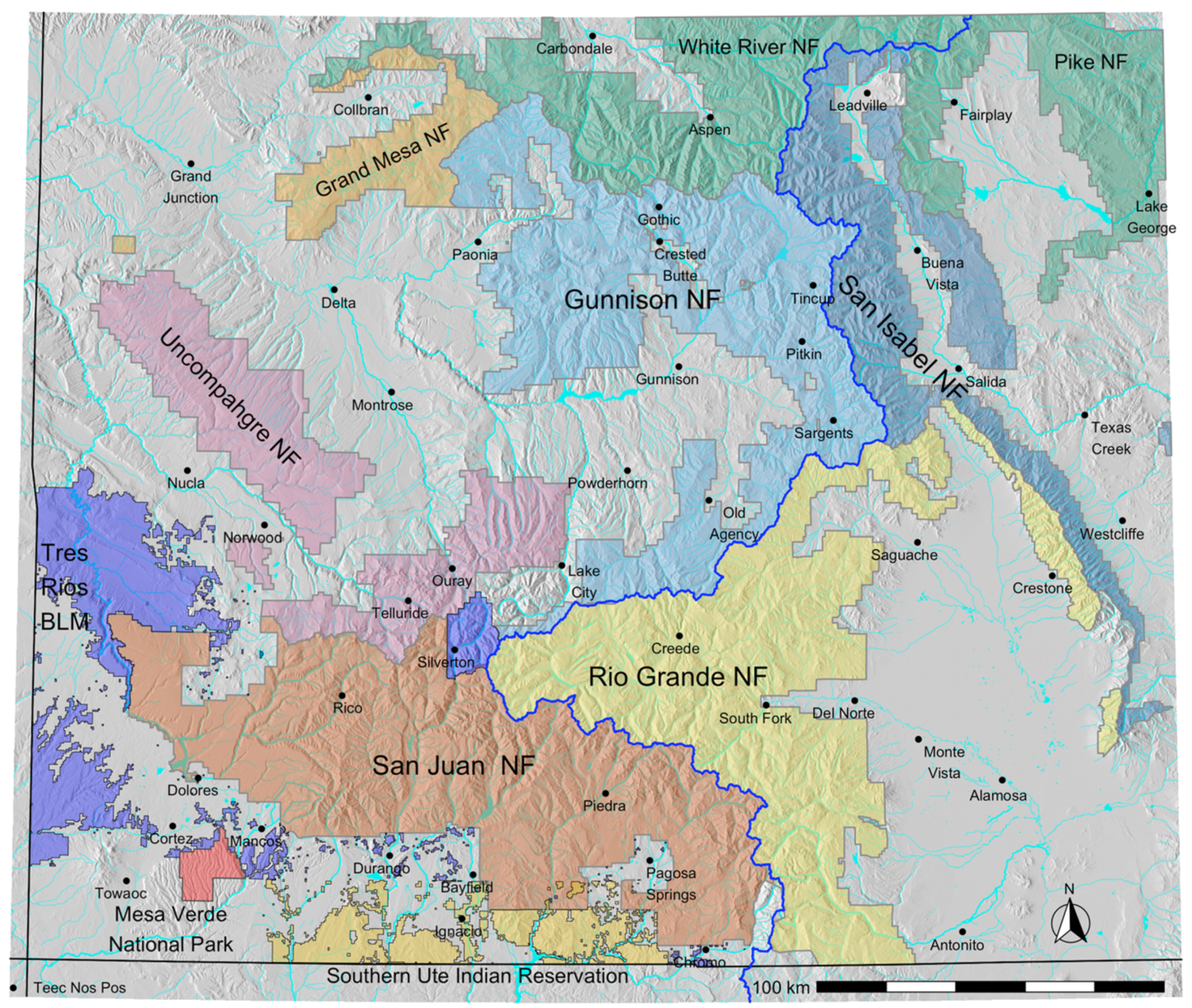
Spatial vegetation data were obtained from 11 land management units within our study area (Figure A1), bounded by longitudes −109.1, −105.3 and latitudes 36.9, 39.45. These data were at the highest resolution used by these organizations for management purposes. There were 299,071 polygons, varying in size from 1.2 × 10⁻⁴ to 11,728 ha, with a median of 7.9. The 11 organizations cover 50.3% of the study area. The area not covered was mostly steppe, grassland, or agricultural, containing little forest.
Figure A1.
Modeled area in southwestern Colorado, showing the land management units whose spatial vegetation data were sampled for the study. Blue line is the Continental Divide.
Figure A1.
Modeled area in southwestern Colorado, showing the land management units whose spatial vegetation data were sampled for the study. Blue line is the Continental Divide.

Appendix A.1.1. National Forest System
For national forest data (including Tres Rios BLM, whose data are maintained together with San Juan NF), we used two geodatabases, the regional R2_FSVeg_Spatial and national USvegNRIS. In the regional database, we searched the DLF and MLF (dominant and majority life form) species fields. Any species in those six fields was considered present in the associated polygon; otherwise, it was considered absent. Presence was supplemented with the national database, NRIS_VegSubpopulations table, SPECIES_SYMBOL field that is used to indicate presence of each species, with multiple records per polygon. We found no species data in the few polygons of the Carson NF inside our window. In the few polygons of the Manti-La Sal NF, most had species codes in the NRIS_VegSubpopulations field SUBGROUP_1, so those were used to indicate presence/absence.
The floor of the San Luis Valley, not part of the Rio Grande NF, contained very large polygons (>12,000 ha). Most of them had no vegetation data; one had several tree species represented, although most of the polygon was treeless. Those polygons were deleted.
For the Uncompagre NF, 78 polygons around Ouray known to have ABCO were set to “present” for that species, because this species was erroneously not represented in the vegetation data.
The PICO that occurs in the Uncompahgre, San Juan, and southern Rio Grande NFs is all composed of plantations outside of the native range. In the shapefile, we set PICO to “absent” in these areas, west of longitude −107.4 or south of latitude 37.7.
Appendix A.1.2. Southern Ute Indian Tribe
Vegetation data for Southern Ute lands were recorded as forest types. Species were assigned to the forest types by a set of rules developed for us by foresters representing the Tribe and Bureau of Indian Affairs. Species, which could be present or absent for a type, were assigned “NA” for that type. When building models for a given species, any sample points showing “NA” for that species were first deleted.
Appendix A.1.3. Mesa Verde National Park
Vegetation data on Mesa Verde National Park (MVNP) were recorded as vegetation types. We used the most specific, the Base_Class field, and developed rules for each type as for the Southern Ute Indian Tribe. For polygons in developed areas, we assigned NA for any species that occurred anywhere in the park.
Large burned areas in the park were mapped as “post-fire”, and the pre-existing vegetation was not indicated. However, the best data for our purposes are the vegetation that grew there recently, even if it is currently absent. Therefore, MVNP provided supplemental files including a 1996 vegetation shapefile, together with data from 147 vegetation plots in the park. For the post-fire polygons from the main shapefile, we substituted polygons for the same areas from the 1996 shapefile with associated vegetation attributes.
To take advantage of the plot data, we extracted the presence of tree species noted in each plot. Because the plot is a small part of the polygon in many cases, plot data were used to assign presence but not absence. Plot coordinates were used to identify the polygon containing each plot and to assign the corresponding presence data to each polygon. If the polygon already had presence for a species based on shapefile attributes, it was unchanged.
Appendix A.2. Sample Points
All shapefiles containing presence–absence data for each species were sampled with a grid of points. For Southern Ute and Mesa Verde shapefiles, we used a grid interval of 0.0023 degrees. For the remainder, which represent large areas, we used a slightly larger interval, 0.0025 degrees (grid interval about 219 × 277 m in our area). Each point was assigned presence–absence data of the polygon over which it fell for all 14 species. This process assured sampling proportional to area and covered the topography thoroughly. The final count of sample points from vegetation shapefiles was 840,069, distributed among units, as shown in Table A1.
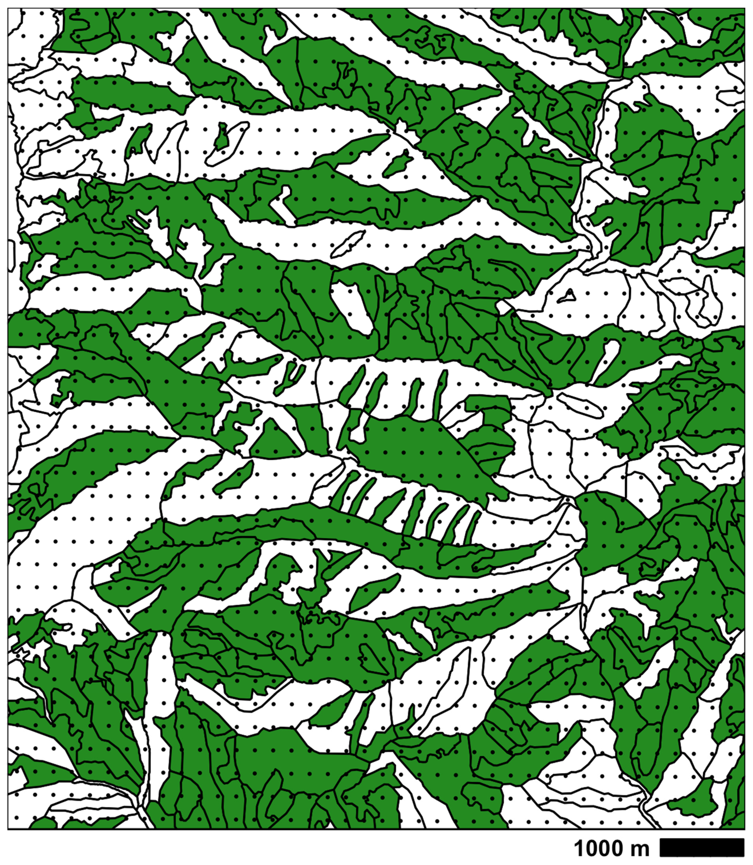
Figure A2 illustrates sampling intensity (dots) within polygons describing the presence and absence of P. tremuloiders within an area of about 80 km2 (10 × 8 km) of high elevational diversity and of fine-scale mapping of polygons. In considering that aspect and slope add additional topographic diversity, it becomes obvious that a fine-grained sampling intensity is required to represent plant distributions in the mountains of our study region.
On the San Juan NF, ABCO and ABLA were confused during automated analysis of satellite imagery to populate the vegetation data. The result was that ABCO appears to exist much higher in elevation than it does, all the way to the Continental Divide. To correct this, on the San Juan NF, any points above 3000 m (approximate upper limit of ABCO at this latitude) that contained ABCO in the vegetation attributes were set to ABLA being present and ABCO absent. This resulted in 746 new ABLA points and dropped 12,853 ABCO points.
Figure A2.
An example of vegetation polygons and their sampling from the San Juan National Forest. Shading indicates presence of Populus tremuloides; black dots indicate a sampling grid with spacing of 0.0025 degrees. At this scale, presence/absence is strongly influenced by topography. Elevation of the map ranges from 2390 to 3530 m.

Appendix A.3. FIA Plots
Sample points from spatial vegetation data were supplemented with data from FIA plots. As a supplement, FIA plots are attractive because they offer accurate species identification and complete census on about 0.17 acre (subplots were lumped in each plot). Additionally, they occur on all land ownerships. In addition, outside our window, they provide access to vegetation data for climates that do not currently occur in the window, but are projected to occur in the future.
We retrieved complete FIA plot records for six states (AZ, CA, CO, NM, NV, UT) in August and September 2015. We eliminated any plot sample records before 2002 and any plots with PLOT_STATUS 3 (not sampled, may or may not have forest). We eliminated duplicate plot records so each plot was represented only once. We dropped plots that had any condition 4 (census water). To focus on the southwestern desert climates, in Nevada, we dropped plots north of latitude 38.5; in California, we dropped plots west of longitude −118.3.
We then compared the provided elevation of the true location with the 90 m DEM elevation of the public (fuzzed/swapped) location. We removed plots with more than 50 m discrepancy, on the assumption that those were fuzzed or swapped to a greater distance. All remaining plots inside our study area window were kept and used as training data.
In preliminary trials, PIED and JUOS appeared to become emergent at lower elevations than where they currently occur in the southern part of the area. We determined that (a) the future climates in these areas do not occur to any extent in the window in the reference period, and (b) these areas were underrepresented in the grid sampling. After obtaining reference climate data for each FIA plot, we filtered the remaining external plots to retain only those that had climates similar to future climates in the desert areas shown as emergent for PIED and JUOS.
We accessed the FIA TREE tables to assemble species presence/absence records for each plot. Because exact locations of FIA plots are secret, FIA staff provided DEM slope and aspect for true locations of each plot. The final count was 7280 FIA plots: 2633 inside the window and 4647 outside. All FIA plots were placed in the pool of points to be sampled as training data.
Appendix A.4. Desert Grid
Because the treeless areas mentioned in Section 4.3 above were not adequately sampled in the management units or FIA plots, we delineated treeless polygons in them (verified with satellite imagery) and established a grid of 7493 points. All data points were assigned “absent” for all tree species.
Appendix A.5. Total Sample
There were 854,842 points available for training the models, including 840,069 from spatial vegetation datasets (Table A1), 7280 FIA plots, and 7493 from the supplemental desert grid.

Table A1.
Number of grid points sampling spatial vegetation data in each management unit, totaling 840,069.
Table A1.
Number of grid points sampling spatial vegetation data in each management unit, totaling 840,069.
| Management Unit | Number of Points |
|---|---|
| Grand Mesa NF | 25,372 |
| Gunnison NF | 122,873 |
| Uncompahgre NF | 75,031 |
| Manti-La Sal NF | 167 |
| Pike NF | 48,305 |
| Rio Grande NF | 147,376 |
| San Isabel NF | 67,581 |
| San Juan NF and Tres Rios BLM | 252,779 |
| White River NF | 71,656 |
| Mesa Verde National Park | 5728 |
| Southern Ute Indian Tribe | 23,201 |
NF, National Forest. BLM, Bureau of Land Management.
Appendix B. Influence of Heatload as a Predictor of Species Occurrence in Reference Period
As explained in the manuscript, instead of using two vectors to represent effects of slope and aspect, as done previously, we convert aspect and slope to heatload (which also incorporates latitude). This variable was the second or third most important descriptor of the climatic niche of all 14 species. To demonstrate heatload’s influence on predicting a suitable niche, we developed for four species (PIAR, PIEN, POTR5, and PIPO, see Table 1) niche models that did not include heatload as a predictor, using only the 11 climate variables of the bioclimate model (Table 2). Despite the high importance of heatload in the bioclimate models (Table 2), out-of-bag errors of models without heatload were only slightly higher than those of Table 5; for PIAR, 0.4%; PIEN 0.8%; POTR5 1.0%, and PIPO 0.3%.
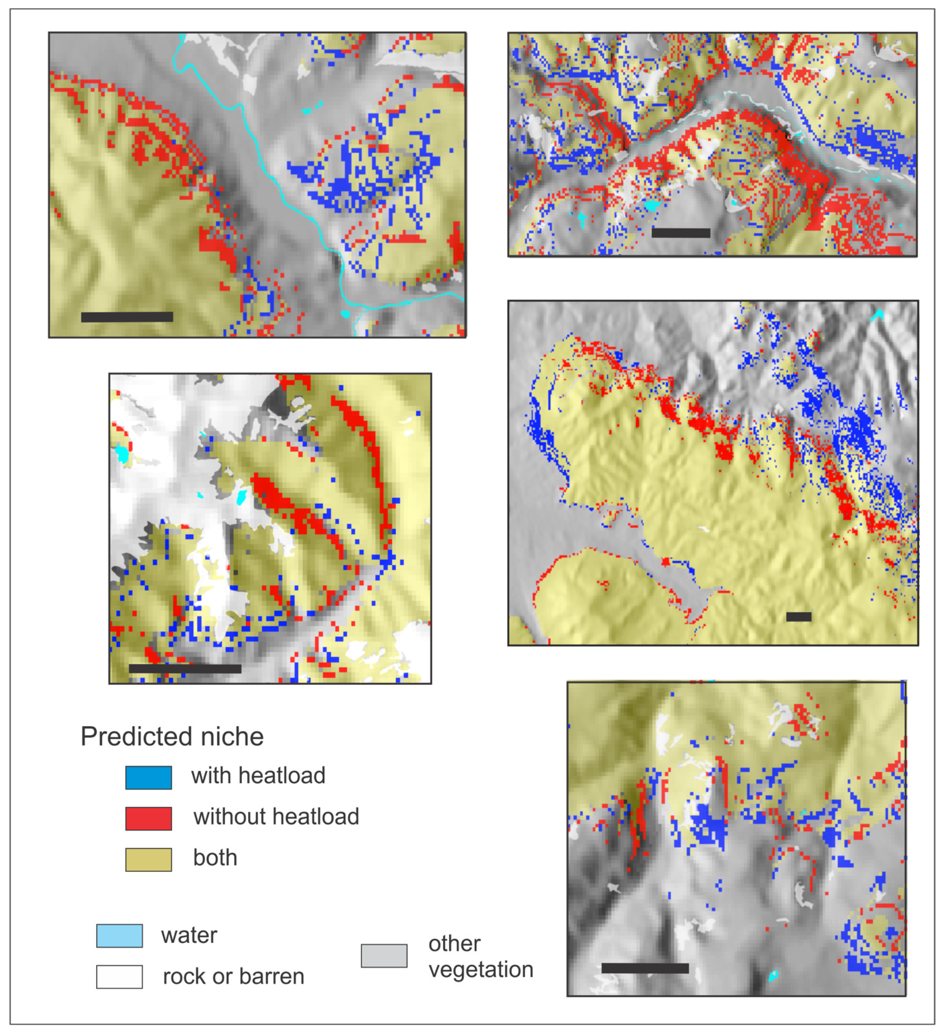
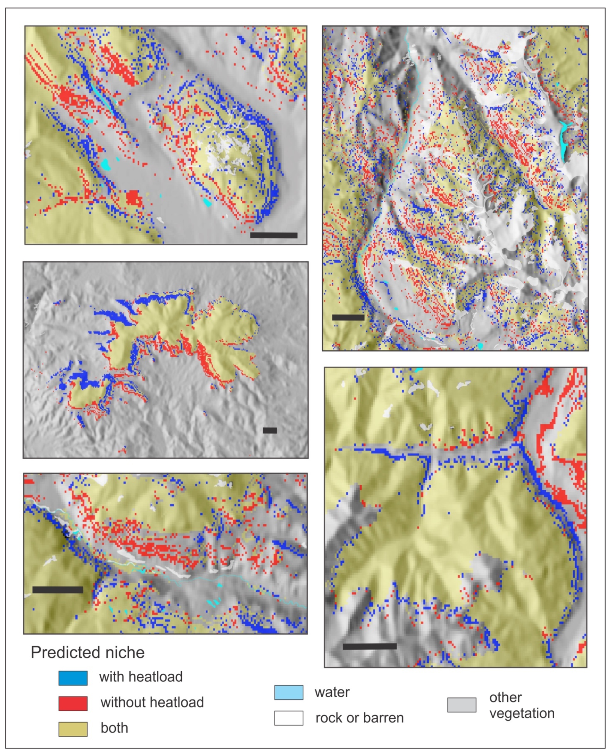
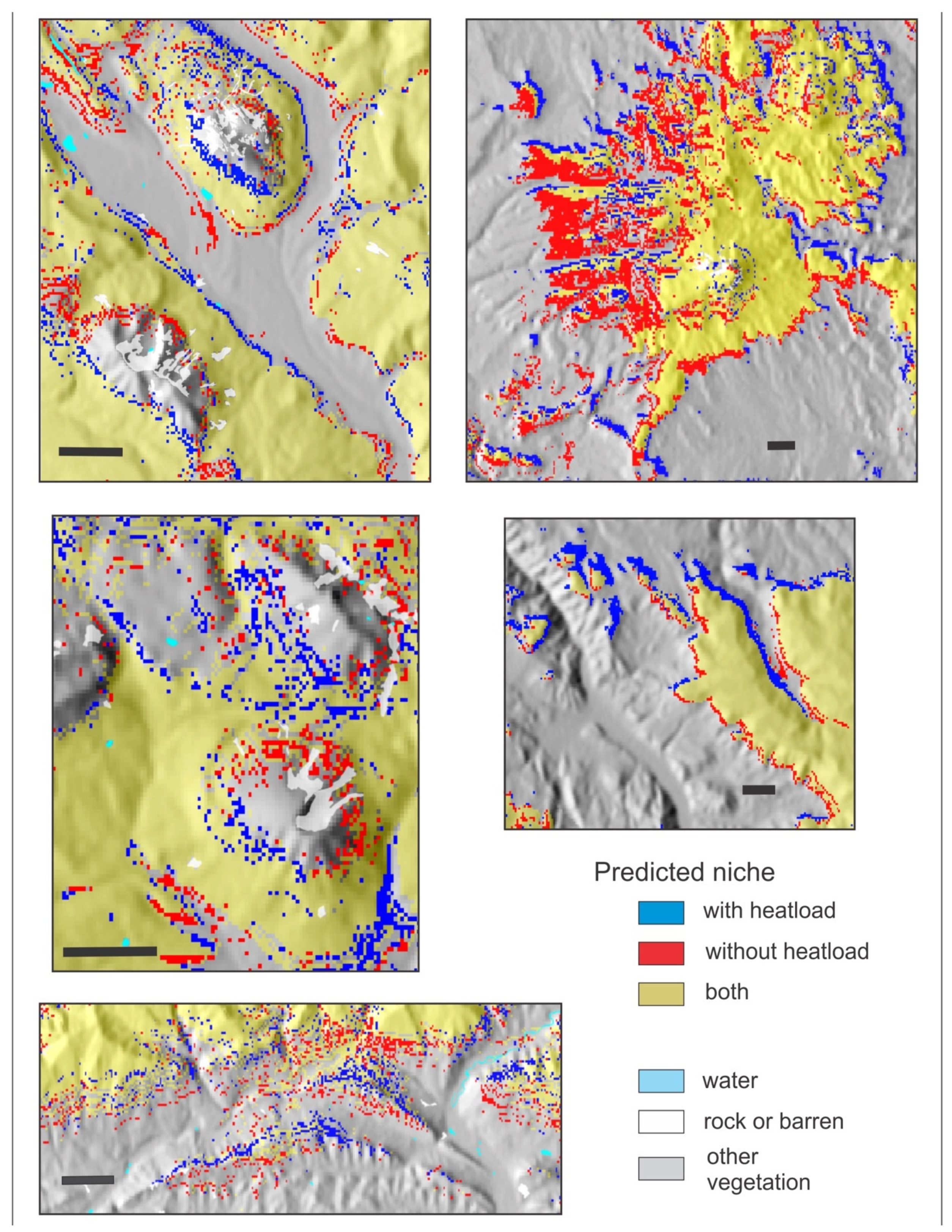
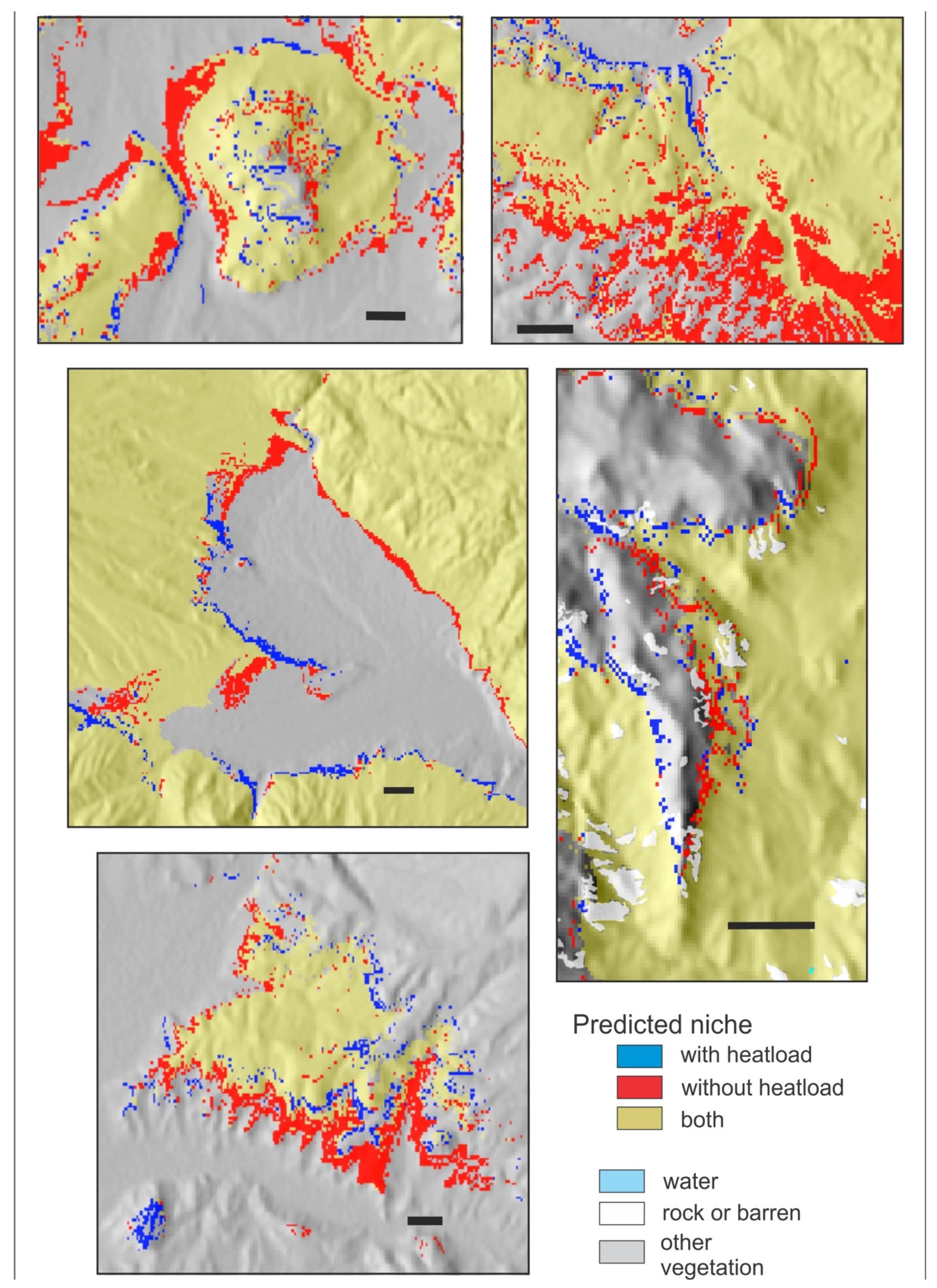
Nonetheless, Figure A3, Figure A4, Figure A5 and Figure A6 illustrate the influence of heatload in fine-tuning topographic effects on the distributions of these four species. In each figure, pixels colored red can be considered those removed when heatload is added to a climatically driven model. The pixels colored blue are those added. For PIAR, a species of the forests at the highest elevations (Table 2), addition of heatload tends to add suitability on warm southern and southwestern aspects and remove it on cool northerly aspects (Figure A3). For PIEN, another subalpine species but with a broader altitudinal distribution, heatload tends to add suitability on cool northerly aspects and remove it on warm southern and southwestern aspects; the effect is most notable for sites near the valley floor or low on the slope (Figure A4). For POTR5 (Figure A5), a species with a broad distribution through the montane and subalpine forests, heatload adds suitability on warm exposures and subtracts suitability on cool exposures near upper timberline, but these effects are reversed lower on the slope and in the valleys. For PIPO (Figure A6), a species of the montane forests, heatload removes suitability in broad swaths on warm sites near the lower limits of distribution while adding suitability on cool sites; but at the upper limits of distribution, the effects are reversed, as heatload adds suitability on the warm exposures but reduces it on the northerly aspects.
Figure A3.
Reference period predicted niche of Pinus aristata from two random forests classification trees illustrating the effects of heatload as a predictor. Gold, niche predicted by both models; red, predicted by 11 climate variables; blue, predicted by the climate variables plus heatload. Scale bar in each panel is 2 km.

Figure A4.
Reference period predicted niche of Picea engelmannii from two random forests classification trees illustrating the effects of heatload as a predictor. Gold, niche predicted by both models; red, predicted by 11 climate variables; blue, predicted by the climate variables plus heatload. Scale bar in each panel is 2 km.

Figure A5.
Reference period predicted niche of Populus tremuloides from two random forests classification trees illustrating the effects of heatload as a predictor. Gold, niche predicted by both models; red, predicted by 11 climate variables; blue, predicted by the climate variables plus heatload. Scale bar in each panel is 2 km.

Figure A6.
Reference period predicted niche of Pinus ponderosa from two random forests classification trees illustrating the effects of heatload as a predictor. Gold, niche predicted by both models; red, predicted by 11 climate variables; blue, predicted by the climate variables plus heatload. Scale bar in each panel is 2 km.

References
- Sturrock, R.N.; Frankel, S.J.; Brown, A.V.; Hennon, P.E.; Kliejunas, J.T.; Lewis, K.J.; Worrall, J.J.; Woods, A.J. Climate Change and Forest Diseases. Plant Pathol. 2011, 60, 133–149. [Google Scholar] [CrossRef]
- Hennon, P.E.; Frankel, S.J.; Woods, A.J.; Worrall, J.J.; Ramsfield, T.D.; Zambino, P.J.; Shaw, D.C.; Ritóková, G.; Warwell, M.V.; Norlander, D.; et al. Applications of a Conceptual Framework to Assess Climate Controls of Forest Tree Diseases. For. Pathol. 2021, e12719. [Google Scholar] [CrossRef]
- Weed, A.S.; Ayres, M.P.; Hicke, J.A. Consequences of Climate Change for Biotic Disturbances in North American Forests. Ecol. Monogr. 2013, 83, 441–470. [Google Scholar] [CrossRef]
- Augspurger, C.K. Reconstructing Patterns of Temperature, Phenology, and Frost Damage over 124 Years: Spring Damage Risk Is Increasing. Ecology 2013, 94, 41–50. [Google Scholar] [CrossRef]
- Reyes-Fox, M.; Steltzer, H.; Trlica, M.J.; McMaster, G.S.; Andales, A.A.; LeCain, D.R.; Morgan, J.A. Elevated CO2 Further Lengthens Growing Season under Warming Conditions. Nature 2014, 510, 259–262. [Google Scholar] [CrossRef] [PubMed]
- Iverson, L.; Prasad, A.; Matthews, S. Modeling Potential Climate Change Impacts on the Trees of the Northeastern United States. Mitig. Adapt. Strateg. Glob. Chang. 2008, 13, 487–516. [Google Scholar] [CrossRef]
- Hamann, A.; Wang, T. Potential Effects of Climate Change on Ecosystem and Tree Species Distribution in British Columbia. Ecology 2006, 87, 2773–2786. [Google Scholar] [CrossRef] [Green Version]
- Rehfeldt, G.E.; Crookston, N.L.; Warwell, M.V.; Evans, J.S. Empirical Analyses of Plant-Climate Relationships for the Western United States. Int. J. Plant Sci. 2006, 167, 1123–1150. [Google Scholar] [CrossRef]
- Gómez-Pineda, E.; Sáenz-Romero, C.; Ortega-Rodríguez, J.M.; Blanco-García, A.; Madrigal-Sánchez, X.; Lindig-Cisneros, R.; Lopez-Toledo, L.; Pedraza-Santos, M.E.; Rehfeldt, G.E. Suitable Climatic Habitat Changes for Mexican Conifers along Altitudinal Gradients under Climatic Change Scenarios. Ecol. Appl. 2020, 30, e02041. [Google Scholar] [CrossRef]
- Rehfeldt, G.E.; Crookston, N.L.; Sáenz-Romero, C.; Campbell, E.M. North American Vegetation Model for Land-Use Planning in a Changing Climate: A Solution to Large Classification Problems. Ecol. Appl. 2012, 22, 119–141. [Google Scholar] [CrossRef] [PubMed]
- Wang, T.; Campbell, E.M.; O’Neill, G.A.; Aitken, S.N. Projecting Future Distributions of Ecosystem Climate Niches: Uncertainties and Management Applications. For. Ecol. Manag. 2012, 279, 128–140. [Google Scholar] [CrossRef]
- Bürger, R.; Lynch, M. Evolution and Extinction in a Changing Environment: A Quantitative-genetic Analysis. Evolution 1995, 49, 151–163. [Google Scholar] [CrossRef] [PubMed]
- Davis, M.B.; Shaw, R.G.; Etterson, J.R. Evolutionary Responses to Changing Climate. Ecology 2005, 86, 1704–1714. [Google Scholar] [CrossRef]
- Rehfeldt, G.E.; Ying, C.C.; Spittlehouse, D.L.; Hamilton, D.A. Genetic Responses to Climate in Pinus Contorta: Niche Breadth, Climate Change, and Reforestation. Ecol. Monogr. 1999, 69, 375–407. [Google Scholar] [CrossRef]
- Rehfeldt, G.E.; Wykoff, W.R.; Ying, C.C. Physiologic Plasticity, Evolution, and Impacts of a Changing Climate on Pinus contorta. Clim. Chang. 2001, 50, 355–376. [Google Scholar] [CrossRef]
- Hagerman, S.M.; Pelai, R. Responding to Climate Change in Forest Management: Two Decades of Recommendations. Front. Ecol. Environ. 2018, 16, 579–587. [Google Scholar] [CrossRef]
- Rehfeldt, G.E.; Jaquish, B.C. Ecological Impacts and Management Strategies for Western Larch in the Face of Climate-Change. Mitig. Adapt. Strateg. Glob. Chang. 2010, 15, 283–306. [Google Scholar] [CrossRef]
- Sáenz-Romero, C.; Lindig-Cisneros, R.A.; Joyce, D.G.; Beaulieu, J.; St Clair, J.B.; Jaquish, B.C. Assisted Migration of Forest Populations for Adapting Trees to Climate Change. Rev. Chapingo Ser. Cienc. For. Ambiente 2016, XXII, 303–323. [Google Scholar] [CrossRef]
- Gray, L.K.; Gylander, T.; Mbogga, M.S.; Chen, P.-Y.; Hamann, A. Assisted Migration to Address Climate Change: Recommendations for Aspen Reforestation in Western Canada. Ecol. Appl. 2011, 21, 1591–1603. [Google Scholar] [CrossRef] [PubMed]
- Machar, I.; Vlckova, V.; Bucek, A.; Vozenilek, V.; Salek, L.; Jerabkova, L. Modelling of Climate Conditions in Forest Vegetation Zones as a Support Tool for Forest Management Strategy in European Beech Dominated Forests. Forests 2017, 8, 82. [Google Scholar] [CrossRef] [Green Version]
- Ackerly, D.D.; Kling, M.M.; Clark, M.L.; Papper, P.; Oldfather, M.F.; Flint, A.L.; Flint, L.E. Topoclimates, Refugia, and Biotic Responses to Climate Change. Front. Ecol. Environ. 2020, 18, 288–297. [Google Scholar] [CrossRef]
- Rehfeldt, G.E.; Worrall, J.J.; Marchetti, S.B.; Crookston, N.L. Adapting Forest Management to Climate Change Using Bioclimate Models with Topographic Drivers. Forestry 2015, 88, 528–539. [Google Scholar] [CrossRef] [Green Version]
- Brown, D.E.; Reichenbacher, F.; Franson, S.E. A Classification of North American Biotic Communities; University of Utah Press: Salt Lake City, UT, USA, 1998; ISBN 978-0-87480-562-8. [Google Scholar]
- Eilperin, J.; Van Houten, C.; Muyskens, J. This Giant Climate Hot Spot Is Robbing the West of Its Water. 2020. Available online: https://wapo.st/2c-colorado (accessed on 24 October 2021).
- NCEI GIS Agile Team. NCEI GIS Map Portal, U.S. Climate Normals Data Map (2006–2020). National Oceanic and Atmospheric Administration, National Centers for Environmental Information. Available online: https://gis.ncdc.noaa.gov/maps/ncei/normals (accessed on 4 July 2021).
- Anonymous. Climate Normals, 1961–1990. National Oceanic and Atmospheric Administration, National Centers for Environmental Information. Available online: https://www1.ncdc.noaa.gov/pub/data/normals/1961-1990/ (accessed on 4 July 2021).
- Breshears, D.D.; Cobb, N.S.; Rich, P.M.; Price, K.P.; Allen, C.D.; Balice, R.G.; Romme, W.H.; Kastens, J.H.; Floyd, M.L.; Belnap, J. Regional Vegetation Die-off in Response to Global-Change-Type Drought. Proc. Natl. Acad. Sci. USA 2005, 102, 15144–15148. [Google Scholar] [CrossRef] [Green Version]
- Rehfeldt, G.E.; Ferguson, D.E.; Crookston, N.L. Aspen, Climate, and Sudden Decline in Western USA. For. Ecol. Manag. 2009, 258, 2353–2364. [Google Scholar] [CrossRef]
- Worrall, J.J.; Rehfeldt, G.E.; Hamann, A.; Hogg, E.H.; Marchetti, S.B.; Michaelian, M.; Gray, L.K. Recent Declines of Populus tremuloides in North America Linked to Climate. For. Ecol. Manag. 2013, 299, 35–51. [Google Scholar] [CrossRef]
- Anonymous. Statistics. National Interagency Fire Center. Available online: https://www.nifc.gov/fire-information/statistics (accessed on 2 July 2021).
- Ingold, J. Five Charts That Show Where 2020 Ranks in Colorado Wildfire History. Before 2002, Colorado Never Had a 100,000-Acre Wildfire. Now It Has Its First 200,000-Acre Fire. 2020. Available online: https://coloradosun.com/2020/10/20/colorado-largest-wildfire-history/ (accessed on 5 June 2021).
- Woodward, F.I. Climate and Plant Distribution; Cambridge Studies in Ecology; Cambridge University Press: Cambridge, UK; New York, NY, USA, 1987; ISBN 978-0-521-23766-6. [Google Scholar]
- Williams, J.W.; Shuman, B.N.; Webb, T.; Bartlein, P.J.; Leduc, P.L. Late-Quaternary Vegetation Dynamics in North America: Scaling from Taxa to Biomes. Ecol. Monogr. 2004, 74, 309–334. [Google Scholar] [CrossRef] [Green Version]
- Jump, A.S.; Hunt, J.M.; Peñuelas, J. Rapid Climate Change-Related Growth Decline at the Southern Range Edge of Fagus sylvatica. Glob. Chang. Biol. 2006, 12, 2163–2174. [Google Scholar] [CrossRef] [Green Version]
- Conlisk, E.; Castanha, C.; Germino, M.J.; Veblen, T.T.; Smith, J.M.; Kueppers, L.M. Declines in Low-Elevation Subalpine Tree Populations Outpace Growth in High-Elevation Populations with Warming. J. Ecol. 2017, 105, 1347–1357. [Google Scholar] [CrossRef] [Green Version]
- Brusca, R.C.; Wiens, J.F.; Meyer, W.M.; Eble, J.; Franklin, K.; Overpeck, J.T.; Moore, W. Dramatic Response to Climate Change in the Southwest: Robert Whittaker’s 1963 Arizona Mountain Plant Transect Revisited. Ecol. Evol. 2013, 1–13. [Google Scholar] [CrossRef]
- Woodall, C.W.; Oswalt, C.M.; Westfall, J.A.; Perry, C.H.; Nelson, M.D.; Finley, A.O. An Indicator of Tree Migration in Forests of the Eastern United States. For. Ecol. Manag. 2009, 257, 1434–1444. [Google Scholar] [CrossRef]
- Kelly, A.E.; Goulden, M.L. Rapid Shifts in Plant Distribution with Recent Climate Change. Proc. Natl. Acad. Sci. USA 2008, 105, 11823–11826. [Google Scholar] [CrossRef] [Green Version]
- Beauregard, F.; de Blois, S. Beyond a Climate-Centric View of Plant Distribution: Edaphic Variables Add Value to Distribution Models. PLoS ONE 2014, 9, e92642. [Google Scholar] [CrossRef]
- Rondeau, R.; Neely, B.; Bidwell, M.; Rangwala, I.; Yung, L.; Clifford, K.; Schulz, T. Spruce-Fir Landscape: Upper Gunnison River Basin, Colorado. Social-Ecological Climate Resilience Project; North Central Climate Science Center: Fort Collins, CO, USA, 2017. [Google Scholar]
- Burrill, E.A.; DiTommason, A.M.; Turner, J.A.; Pugh, S.A.; Menlove, J.; Christiansen, G.; Perry, C.J.; Conkling, B.L. The Forest Inventory and Analysis Database: Database Description and User Guide for Phase 2 (Version 9.0.1); USDA Forest Service: Washington DC, USA, 2021.
- Jarvis, A.; Reuter, H.I.; Nelson, A.; Guevara, E. Hole-Filled Seamless SRTM Data V4, International Centre for Tropical Agriculture (CIAT). Available online: https://srtm.csi.cgiar.org (accessed on 11 December 2021).
- Crookston, N.L.; Rehfeldt, G.E. Climate Estimates and Plant-Climate Relationships: Custom Climate Data Requests. Research on Forest Climate Change: Potential Effects of Global Warming on Forests and Plant Climate Relationships in Western North America and Mexico. Available online: https://charcoal2.cnre.vt.edu/climate/customData/ (accessed on 22 November 2021).
- Rehfeldt, G.E. A Spline Model of Climate for the Western United States. General Technical Report RMRS-GTR-165; USDA Forest Service, Rocky Mountain Research Station: Fort Collins, CO, USA, 2006.
- McCune, B.; Keon, D. Equations for Potential Annual Direct Incident Radiation and Heat Load. J. Veg. Sci. 2002, 13, 603–606. [Google Scholar] [CrossRef]
- Breiman, L. Random Forests. Mach. Learn. 2001, 45, 5–32. [Google Scholar] [CrossRef] [Green Version]
- Huang, B.F.F.; Boutros, P.C. The Parameter Sensitivity of Random Forests. BMC Bioinform. 2016, 17, 331. [Google Scholar] [CrossRef] [PubMed] [Green Version]
- Liaw, A.; Wiener, M. Classification and Regression by RandomForest. R News 2002, 2, 18–22. [Google Scholar]
- Van Vuuren, D.P.; Edmonds, J.; Kainuma, M.; Riahi, K.; Thomson, A.; Hibbard, K.; Hurtt, G.C.; Kram, T.; Krey, V.; Lamarque, J.-F. The Representative Concentration Pathways: An Overview. Clim. Chang. 2011, 109, 5–31. [Google Scholar] [CrossRef]
- Turesson, G. The Plant Species in Relation to Habitat and Climate: Contributions to the Knowledge of Genecological Units. Hereditas 1925, 6, 147–236. [Google Scholar] [CrossRef]
- Rehfeldt, G.E.; Leites, L.P.; Joyce, D.G.; Weiskittel, A.R. Role of Population Genetics in Guiding Ecological Responses to Climate. Glob. Chang. Biol. 2017. [CrossRef] [PubMed]
- Rehfeldt, G.E.; Jaquish, B.C.; Sáenz-Romero, C.; Joyce, D.G.; Leites, L.P.; Bradley St Clair, J.; López-Upton, J. Comparative Genetic Responses to Climate in the Varieties of Pinus ponderosa and Pseudotsuga menziesii: Reforestation. For. Ecol. Manag. 2014, 324, 147–157. [Google Scholar] [CrossRef]
- Williams, J.W.; Jackson, S.T.; Kutzbach, J.E. Projected Distributions of Novel and Disappearing Climates by 2100 AD. Proc. Natl. Acad. Sci. USA 2007, 104, 5738–5742. [Google Scholar] [CrossRef] [Green Version]
- Jackson, S.T.; Overpeck, J.T. Responses of Plant Populations and Communities to Environmental Changes of the Late Quaternary. Paleobiology 2000, 26, 194–220. [Google Scholar] [CrossRef]
- Vose, J.M.; Peterson, D.L.; Patel-Weynand, T. Effects of Climatic Variability and Change on Forest Ecosystems: A Comprehensive Science Synthesis for the U.S. Forest Sector; General Technical Report PNW-GTR-870; US Forest Service, Pacific Northwest Research Station: Portland, OR, USA, 2012.
- Prasad, A.; Pedlar, J.; Peters, M.; McKenney, D.; Iverson, L.; Matthews, S.; Adams, B. Combining US and Canadian Forest Inventories to Assess Habitat Suitability and Migration Potential of 25 Tree Species under Climate Change. Divers. Distrib. 2020, 26, 1142–1159. [Google Scholar] [CrossRef]
Figure 1.
Modeled study area in the Southern Rocky Mountains, southwestern Colorado. Blue line is the Continental Divide. Area is 94,238 km2.
Figure 1.
Modeled study area in the Southern Rocky Mountains, southwestern Colorado. Blue line is the Continental Divide. Area is 94,238 km2.

Figure 2.
Changes in mean annual temperature and precipitation in the study area between the reference period and the decade around 2060, as projected by the 11 climate scenarios. The mean of all scenarios is represented by “+”.
Figure 2.
Changes in mean annual temperature and precipitation in the study area between the reference period and the decade around 2060, as projected by the 11 climate scenarios. The mean of all scenarios is represented by “+”.

Figure 3.
Modeled niche area of species by elevation in reference period and the decade around 2060. Each 100 m elevation class is represented by two columns, one for the reference period and one for 2060. The latter represents the optimistic niche area including threatened habitat (orange); the black portion is the secure niche area, with only persistent and emergent.

Figure 4.
Distribution of change classes in the full model extent for Picea engelmannii, representing projected changes between the reference period (1961–1990) and the decade around 2060 mapped on 90 m gridded DEM.
Figure 4.
Distribution of change classes in the full model extent for Picea engelmannii, representing projected changes between the reference period (1961–1990) and the decade around 2060 mapped on 90 m gridded DEM.

Figure 5.
Two hypothetical project areas and change projections of the species suitable in the reference period or 2060. Project A is at relatively high elevation; project B at low elevation. The species maps encompass the full area of the first panel. Note that colors in the first panel (upper left) code elevation; colors in the species maps show the change classes.

Figure 6.
Change classes for Pinus ponderosa on and near the San Juan National Forest. Inset shows only threatened habitat, with color gradient representing percent of votes in the future. Deep green areas represent the most favorable of the threatened habitat.
Figure 6.
Change classes for Pinus ponderosa on and near the San Juan National Forest. Inset shows only threatened habitat, with color gradient representing percent of votes in the future. Deep green areas represent the most favorable of the threatened habitat.

Figure 7.
Projections for Pinus aristata in the area with its most favorable future habitat. (A) Mean votes of the model based on 11 climates, dark green showing the greatest suitability. (B) Areas where 1 or 2 future climates indicate that P. aristata will be suited (votes ≥50%). At most only two climates agree in a small area (12 ha). (C) Change zones (colors as in Figure 6) based on only the single most favorable climate scenario, CNRMCM5, RCP4.5. This shows that most of the projected suitable habitat in B would be persistent, while a small portion would be emergent.

Table 1.
Species used in bioclimate modelling, number of point locations recording presence (which is also the number of presence and absence points used in training the model), median elevation of presence data points, and vegetation associations [23] in which the species occurs.
Table 1.
Species used in bioclimate modelling, number of point locations recording presence (which is also the number of presence and absence points used in training the model), median elevation of presence data points, and vegetation associations [23] in which the species occurs.
| Species | Acronym | Number of Presence Points | Median Elevation (m) | Vegetation Association |
|---|---|---|---|---|
| Juniperus osteosperma (Torr.) Little | JUOS | 66,827 | 2027 | Woodland |
| Pinus edulis Engelm. | PIED | 112,895 | 2135 | Woodland |
| Quercus gambelii Nutt. | QUGA | 148,180 | 2360 | Woodland, montane forest, montane scrub |
| Juniperus scopulorum Sarg. | JUSC2 | 29,034 | 2433 | Woodland, montane forest |
| Pinus ponderosa Douglas ex C. Lawson | PIPO | 147,124 | 2549 | Montane forest |
| Abies concolor (Gord. and Glend.) Lindl. | ABCO | 33,587 | 2671 | Montane forest, subalpine forest |
| Pseudotsuga menziesii (Mirb.) Franco | PSME | 142,639 | 2788 | Montane forest |
| Picea pungens Engelm. | PIPU | 15,049 | 2803 | Subalpine forest |
| Populus tremuloides Michx. | POTR5 | 297,271 | 2903 | Montane forest, subalpine forest |
| Pinus flexilis E.James | PIFL2 | 19,476 | 2984 | Subalpine forest |
| Pinus contorta Douglas ex Loudon | PICO | 70,266 | 3101 | Subalpine forest |
| Pinus aristata Engelm. | PIAR | 31,935 | 3151 | Subalpine forest |
| Picea engelmannii Engelm. | PIEN | 304,310 | 3210 | Subalpine forest |
| Abies lasiocarpa (Hook.) Nutt. | ABLA | 183,434 | 3215 | Subalpine forest |
Table 2.
Climate variables and the frequency of their ranking as the most important variables in predicting the presence of 14 species as measured by the mean decrease in accuracy.
Table 2.
Climate variables and the frequency of their ranking as the most important variables in predicting the presence of 14 species as measured by the mean decrease in accuracy.
| Variable | Definition | Number of Models in which Variable Ranked | ||
|---|---|---|---|---|
| Highest | Upper Two | Upper Four | ||
| dd5 | Degree days > 5 °C (based on mean monthly temperature) | 1 | 1 | 2 |
| map | Mean annual precipitation | 1 | 2 | 3 |
| gsp | Growing season precipitation, April to September | 0 | 1 | 1 |
| mindd0 | Degree days < 0 °C (based on mean minimum monthly temperature) | 2 | 2 | 3 |
| d100 | Julian date on which the sum of degree days > 5 °C reaches 100 | 2 | 2 | 3 |
| tdiff | Temperature difference between warmest and coldest month | 3 | 4 | 13 |
| pratio | Precipitation ratio, growing season to annual: gsp/map | 1 | 3 | 8 |
| mapdd5 | (map × dd5)/1000 | 3 | 5 | 6 |
| adi | Annual dryness index: dd50.5/map | 0 | 0 | 0 |
| adimindd0 | adi × mindd0 | 1 | 2 | 3 |
| sdimindd0 | (gsdd50.5/gsp) × mindd0, where gsdd5 is the degree-day sum between the last freezing temperature of spring and the first freezing temperature of autumn | 0 | 0 | 0 |
| heatload | 0.339 + 0.808 × cos(L) × cos(S) + −0.196 × sin(L) × sin(S) + −0.482 × cos(A) × sin(S), where L = latitude in radians, S = slope in radians, A = aspect in radians, rotated and folded such that minimum values are at 45°and maximum values at 225° [45] | 0 | 6 | 14 |
Table 3.
Habitat change classes based on votes generated by models using reference period climate and eleven 2060 climates.
Table 3.
Habitat change classes based on votes generated by models using reference period climate and eleven 2060 climates.
| Change Classes | Proportion of Votes | Interpretation | |
|---|---|---|---|
| Reference Period | Post Mid-Century | ||
| Always unsuitable | <0.5 | <0.5 | Climate is unsuitable in reference period and remains unsuitable in the future |
| Lost | ≥0.5 | <0.3 | Future climate will be so unfavorable that the species is unlikely to survive the century |
| Threatened | ≥0.5 | ≥0.3 to <0.5 | Future climate will be unfavorable but the species may survive under otherwise favorable conditions |
| Persistent | ≥0.5 | ≥0.5 | Future climate will remain suitable |
| Emergent | <0.5 | ≥0.5 | Areas outside current distribution that will become climatically suitable |
Table 4.
Errors of fit (%) for the developmental models, validation exercises, and final models.
| Species | Developmental Model a | Validation of Developmental Model b | Final Model c | ||||||
|---|---|---|---|---|---|---|---|---|---|
| Out of Bag | Commission | Omission | Total Error | Commission | Omission | Out of Bag | Commission | Omission | |
| JUOS | 6.1 | 6.2 | 3.9 | 6.2 | 6.4 | 3.6 | 5.7 | 5.8 | 4.1 |
| PIED | 8.1 | 8.2 | 6.9 | 8.1 | 8.4 | 6.3 | 7.6 | 7.7 | 7.0 |
| QUGA | 8.6 | 9.1 | 6.0 | 8.7 | 9.3 | 5.8 | 8.2 | 8.6 | 6.5 |
| JUSC2 | 7.8 | 7.9 | 6.1 | 8.0 | 8.0 | 5.8 | 7.2 | 7.2 | 6.1 |
| PIPO | 9.1 | 9.5 | 7.3 | 9.1 | 9.6 | 6.9 | 8.7 | 9.0 | 7.5 |
| ABCO | 5.3 | 5.4 | 2.9 | 5.4 | 5.5 | 2.9 | 4.9 | 5.0 | 3.0 |
| PSME | 14.3 | 14.5 | 13.3 | 14.4 | 14.7 | 12.7 | 13.6 | 13.6 | 13.9 |
| PIPU | 9.8 | 9.8 | 11.0 | 10.1 | 10.1 | 10.5 | 9.4 | 9.4 | 10.5 |
| POTR5 | 15.8 | 16.4 | 14.6 | 15.9 | 16.8 | 14.2 | 15.4 | 15.5 | 15.2 |
| PIFL2 | 9.0 | 9.0 | 5.9 | 9.1 | 9.2 | 5.8 | 8.1 | 8.2 | 6.4 |
| PICO | 6.8 | 7.1 | 3.6 | 6.9 | 7.2 | 3.5 | 6.4 | 6.6 | 3.9 |
| PIAR | 9.2 | 9.3 | 6.1 | 9.5 | 9.6 | 5.5 | 9.0 | 9.1 | 5.8 |
| PIEN | 12.6 | 13.7 | 10.6 | 12.5 | 13.9 | 9.9 | 12.3 | 13.1 | 10.9 |
| ABLA | 13.8 | 14.5 | 11.4 | 14.0 | 14.9 | 10.7 | 13.3 | 13.6 | 12.0 |
a built from a 90% sample of the presence–absence database. b calculated from running the 10% withheld through the developmental model. c built from all data.
Table 5.
Allocation of reference period niches into lost, threatened, and persistent categories, plus emergent, leading to changes in niche area expected in the future. Both niche change columns include emergent as future niche.
Table 5.
Allocation of reference period niches into lost, threatened, and persistent categories, plus emergent, leading to changes in niche area expected in the future. Both niche change columns include emergent as future niche.
| Species a | Reference Period Niche (km2) | Projected Fate of Reference Period Niche (Percent) | Emergent Niche | Niche Change (Percent) | Median Elevation Change (m) d | ||||
|---|---|---|---|---|---|---|---|---|---|
| Lost Area | Threatened Area | Persistent Area | Percent of Reference Period Niche | Area (km2) | Optimistic b | Pessimistic c | |||
| JUOS | 19,198 | 15 | 64 | 21 | 7 | 1263 | −8 | −72 | 27–73 |
| PIED | 26,891 | 17 | 44 | 39 | 43 | 11,528 | +26 | −18 | 235–382 |
| QUGA | 21,919 | 13 | 39 | 48 | 47 | 10,223 | +34 | −6 | 185–311 |
| JUSC2 | 14,349 | 47 | 41 | 12 | 23 | 3239 | −24 | −65 | 214–296 |
| PIPO | 19,553 | 34 | 55 | 10 | 6 | 1144 | −28 | −84 | 126–297 |
| ABCO | 6333 | 76 | 24 | 0 | 1 | 45 | −75 | −99 | 195–316 |
| PSME | 18,862 | 15 | 76 | 9 | 4 | 690 | −12 | −88 | 64–212 |
| PIPU | 7956 | 75 | 25 | 0 | 0 | 0 | −75 | −100 | −44–NA |
| POTR5 | 25,332 | 55 | 43 | 2 | 17 | 4369 | −37 | −80 | 293–639 |
| PIFL2 | 5809 | 100 | 0 e | 0 | 0 | 0 | −100 | −100 | NA |
| PICO | 7980 | 100 | 0 | 0 | 0 | 0 | −100 | −100 | NA |
| PIAR | 7714 | 100 | 0 | 0 | 0 | 0 | −100 | −100 | NA |
| PIEN | 21,530 | 44 | 54 | 2 | 5 | 985 | −39 | −94 | 173–562 |
| ABLA | 15,496 | 56 | 43 | 1 | 5 | 824 | −51 | −94 | 214–597 |
a Sorted by median elevation in the reference period (Table 1). b Assuming survival of trees in threatened class. c Assuming mortality of trees in threatened class. d Elevation change under optimistic to pessimistic assumptions. e Fifty-three cells of PIFL2 (6 × 10⁻⁵ percent of reference area) are threatened.
Table 6.
Changes in forest and woodland niche area projected in the future based on integration of species changes.
Table 6.
Changes in forest and woodland niche area projected in the future based on integration of species changes.
| Change from Reference Period (%) | |||
|---|---|---|---|
| With Emergent | Without Emergent | ||
| With QUGA | |||
| Optimistic a | −4 | −13 | |
| Pessimistic b | −42 | −67 | |
| Without QUGA c | |||
| Optimistic | −9 | −20 | |
| Pessimistic | −56 | −78 | |
a Assuming survival of trees in threatened class. b Assuming mortality of trees in threatened class. c QUGA removed before analysis both in reference period and future.
Publisher’s Note: MDPI stays neutral with regard to jurisdictional claims in published maps and institutional affiliations. |
© 2021 by the authors. Licensee MDPI, Basel, Switzerland. This article is an open access article distributed under the terms and conditions of the Creative Commons Attribution (CC BY) license (https://creativecommons.org/licenses/by/4.0/).
Share and Cite
MDPI and ACS Style
Worrall, J.J.; Rehfeldt, G.E. Strategic Application of Topoclimatic Niche Models in Managing Forest Change. Forests 2021, 12, 1780. https://0-doi-org.brum.beds.ac.uk/10.3390/f12121780
AMA Style
Worrall JJ, Rehfeldt GE. Strategic Application of Topoclimatic Niche Models in Managing Forest Change. Forests. 2021; 12(12):1780. https://0-doi-org.brum.beds.ac.uk/10.3390/f12121780
Chicago/Turabian StyleWorrall, James J., and Gerald E. Rehfeldt. 2021. "Strategic Application of Topoclimatic Niche Models in Managing Forest Change" Forests 12, no. 12: 1780. https://0-doi-org.brum.beds.ac.uk/10.3390/f12121780
Note that from the first issue of 2016, this journal uses article numbers instead of page numbers. See further details here.