
A Study of the Distribution of Forest Density in Inner Mongolia Based on Environmental Factors


Beijing Key Laboratory of Precision Forestry, Beijing Forestry University, Beijing 100089, China
*
Author to whom correspondence should be addressed.
Forests 2022, 13(2), 313; https://0-doi-org.brum.beds.ac.uk/10.3390/f13020313
Submission received: 9 December 2021
/
Revised: 3 February 2022
/
Accepted: 12 February 2022
/
Published: 14 February 2022
(This article belongs to the Special Issue Adaptive Forest Management to Climatic Change)
Abstract
:With the intensification of global climate change, exploring the impact of environmental factors on tree density can provide technical support for sustainable forest management. In this paper, the random forest parameters nTree and mtry were optimized using a particle swarm optimization algorithm. The density, average temperature, soil thickness, forest water consumption, slope, slope direction, slope position, soil type, and diameter at breast height (DBH) of the dominant tree species in Inner Mongolia were fitted using random forest regression with a satisfactory fitting effect ( > 0.60). The results show that the average temperature, soil thickness, and forest water consumption were the main factors restricting tree density, and the influence of each factor changed depending on the stage of tree growth. Based on 2018 forest resource data of the Inner Mongolia Autonomous Region, four diameter class models were used to calculate tree density, and Kriging interpolation was used to form a density distribution grid map of the main tree species according to diameter class toward providing a theoretical basis and data support for afforestation and forest management strategies that are justified according to the available environmental resources.
1. Introduction
Forests are the largest ecosystem on land and play an important role in human survival and development. Therefore, determining how to manage a forest ecosystem so that it can both provide the required products for human beings and perform an effective ecological service is the focus of forestry scientists. In most cases, though, the resources and environmental conditions for stimulating forest growth are limited. Environmental factors such as the distribution of water, temperature, and soil, in combination, are important restrictive factors that determine the forest structure and stand density. This density, which is important for the stability of the ecosystem and biological productivity [1], is the main factor that can be controlled by human beings [2,3] to determine whether the stand structure is sound both quantitatively and qualitatively [4]. Many countries have carried out numerous studies related to the law of stand density distribution, and in our view, the factors affecting stand density can be divided into biotic and abiotic. Most studies on biological factors have explored how population and resource competition between various biological factors, in addition to individual competition, influence stand density [5,6,7,8,9,10], or how abiotic factors in production indices can be combined with biological factors for analysis [11].
Previous studies have mainly used gray system theory [11], genetic algorithm [12], density control model [13], inverse solution [14], variable method, and optimal control theory [15] along with skewness, kurtosis, and a diameter variation coefficient [16] for the modeling of algorithms, and growth and thinning effects [17] according to the methods of Nelder trials [18]. In an analysis of relevant influencing factors, a study of a 25 ha forest sample plot in Taiwan found that specific species will be filtered out that have the traits required for survival in specific habitats. In detail, that study showed that environmental factors have restrictive effects on certain tree species [19], and the effect of habitat on tree survival was studied in a dynamic monitoring sample plot of a 20 ha forest in Xishuangbanna. The results showed that biological and abiotic factors interacted to affect forest density [20]. Studies in the mountainous areas of East and Northeast China found that both biological and abiotic factors affect the density of a forest, but their importance varies according to its life stage [21]. A study on a 16 ha U.S. forest monitoring sample plot found that soil and solar radiation are key factors affecting forest density, exhibiting a significantly positive correlation [22]. A generalized linear mixed-effect model was used in a study of a BCI 50 ha forest sample plot in which the seedling density was found to be related to topographic factors and water along with interspecific differences in water availability [23].
Based on previous studies, we wanted to further explore how forest density is affected by environmental factors, particularly which have the greatest restrictive effect and whether the impact changes in the different growth stages of trees. Based on consideration of the factors found in previous studies combined with the existing data conditions [24], we selected average temperature, forest water consumption, soil thickness, soil type, dominant tree species, slope, slope direction, and slope position as influencing factors, and we examined the rules of their influence on forest density and established a model. A density distribution law of large regions and multi-tree species based on abiotic factors (environmental factors) through a random forest regression algorithm optimized using a particle swarm algorithm had not previously been reported.
Most of the random forest regression models adopted in previous studies chose empirical values for nTree value and mtry value inputs, which have some limitations, whereas the particle swarm algorithm iteratively optimizes the parameters of the random forest regression model [25]. Therefore, with this paper, we established a model of stand density for different size classes in Inner Mongolia using particle cluster algorithm-optimized random forest regression based on 2018 Inner Mongolia forest resource data and MODIS-related meteorological data. We analyzed the contribution ratio of the independent variable and dominant factors that affect forest density, and then used Kriging interpolation to calculate stand density distribution among different DBH zones for each tree species. The goal was to provide a theoretical basis and realistic guidance for forest management to facilitate rational use of the environmental resources in the Inner Mongolia region.
2. Materials and Methods
2.1. Overview of the Study Area
The Inner Mongolia Autonomous Region is the third-largest province in China and located on its northern border. It has a long and narrow shape that extends northeast to southwest. East rises from 126 degrees east to 04′, west to east longitude 97°12′, across longitude 28 degrees 52′, and east–west straight away from more than 2400 km; and south latitude 37 degrees 24′ north, north latitude 53 degrees 23′, longitudinal latitude 15 degrees 59′, and straight distance 1700 km. The total area is 1,183,000 square kilometers, accounting for 12.3% of China’s land area. The Inner Mongolia Autonomous Region is vast and has many complicated landforms, but it is mainly a plateau-type geomorphic area with an average altitude of about 1000 m. According to the 2018 report on China’s forest resources, this region’s forests cover 26,148,500 ha (22.10% coverage), ranking first in the country.
2.2. Forest Data
The forest data in this paper are based on the 2018 forest leaflet data provided by the National Forest Resource intelligence management platform, which was obtained through the Inner Mongolia Autonomous Region Forest Resource Planning Design Survey, also known as a type-two survey, in which all forest resources are classified into multiple subclasses of 0.4–35 ha according to artificial, natural, and comprehensive divisions. The survey took the minor class as the basic unit every 10 years, and to date, the Inner Mongolia Autonomous Region has completed multiple rounds of secondary survey work [26]. The main survey components are land class, forest class, forest species, tree height, plant number density, area, dominant tree species, tree composition, age class, age group, production period, topography factor, soil factor, and site type. Many forest resource factors and operational management factors, such as forest structure, are included.
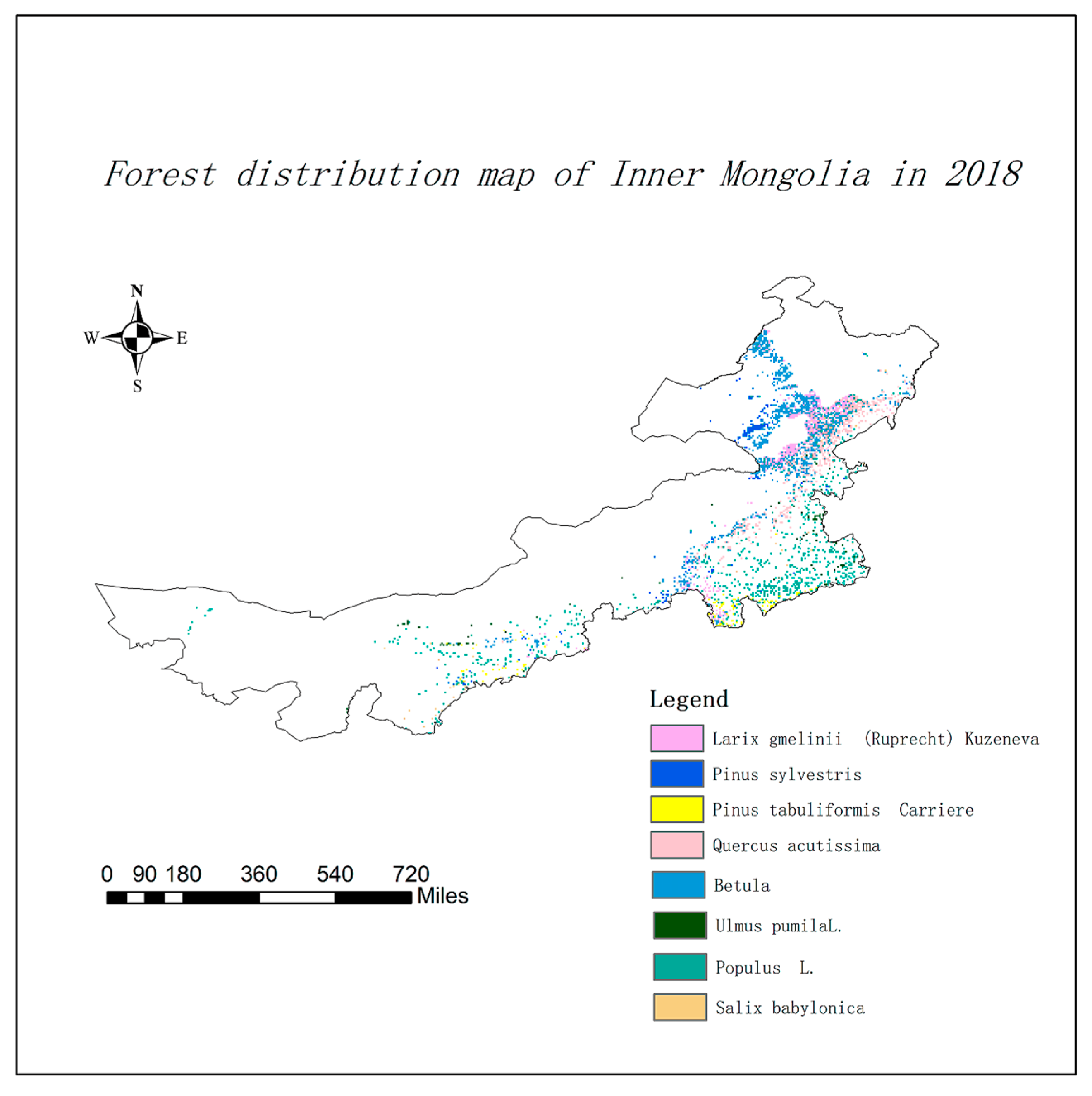
The main tree species and groups of species were selected for density distribution law study by analyzing the 2018 Inner Mongolia forest data: Larix gmelinii (Rupr.) Kuzen., Pinus sylvestris var. mongolica Litv., Pinus tabuliformis Carrière, Quercus L., Betula L., Ulmus pumila L., Populus przewalskii Maxim., and Salix L. The specific distribution is shown in Figure 1. The main tree species were divided into four size classes: 5, 15, 25, and 35 cm. The average chest diameter ranges were 0 to 9.9, 10 to 19.9, 20 to 29.9, and >30 cm, respectively. The distribution range and number of specific forest subclass densities are shown in Table 1.
2.3. Relevant Environmental Factor Data
The Inner Mongolia Autonomous Region spans four climate zones: wet, semi-wet, semi-arid, and arid. In the latter two, windproofing and sand-fixing, prevention of soil and water loss, and conservation of water sources are the main forestation objectives. Macroscopically, water resources and temperature are important for tree growth and development, which participate in and affect the material cycle and energy flow of the forest ecosystem. Water consumption has two components, forest tree transpiration and woodland surface evaporation, which are considered per unit time and area. In this study, plant transpiration, soil evaporation, and canopy intercept evaporation data were taken from the Penman–Monteith–Leuning Evapotranspiration V2 (PML_V2) terrestrial steaming and total primary productivity dataset, accessed from the website “National Tibetan Plateau science data center” (doi:10.11888/geogra.TPDC.270251) [27], with a TIFF data format and spatiotemporal resolution of 8 days, 0.05° for a time span from July 2002 to August 2019.
We used a 2008–2017 PML_V2 dataset of land evaporation and total primary productivity after extraction of the study area as the annual average forest tree water consumption data. Mean temperature data were cited from the Chinese surface temperature dataset (2003–2017) accessed on the website “National Science Data Center on the Tibetan Plateau” (doi:10.5281/zenodo.3528024) [28], which contains monthly surface temperature data from 2003 to 2017 for all of China (approximately 9.6 million km2) at a spatial resolution of 5600 m. A total of 10 years of Chinese surface temperature datasets of the study area from 2008 to 2017 were extracted as mean temperature data by cropping and calculating the study area.
2.4. Data Preprocessing
We used the latitude and longitude of the midpoint of the 2018 forest minor class in the Inner Mongolia Autonomous Region, and from this, the multi-value point tool of arcmap10.2 software was used to extract data on vegetation transpiration, soil evaporation, canopy cut-off evaporation, and surface temperature from 2008 to 2017, which were evaluated using a grid calculator. The completed attribute table data were then exported as Excel files.
Meanwhile, based on the 2018 forest resource data, the data of the woodland minor class from the second type of investigation of forest resources were extracted and exported as Excel files using the ArcGIS software platform, and irrelevant fields were then filtered out of these files in Excel. Data on tree species, slope, slope direction, slope position, mean chest diameter, plant number density, soil type, and soil thickness were retained. Furthermore, normalization of continuous numerical variables was required for mapping data on a suitable scale and for rapid and accurate convergence in the machine learning process, including mean temperature, tree water consumption, plant density, and soil thickness. The normalization formula is shown in Equation (1). In addition, slope, slope direction, slope position, soil type, and dominant tree species were used as categorical variables, and plant density was used as a response variable to participate in the construction of the main tree species density distribution model based on environmental factors.
where i is the number of samples in the dataset variable; are the normalized values; is the minimum value in the dataset ; and is the maximum value in the dataset .
In turn, all the data on vegetation transpiration, including air temperature meteorology and forest resources, were read in Excel, and the integration of multi-dimensional information—forest water consumption, surface mean air temperature, slope, slope direction, slope position, soil type, soil thickness, mean chest diameter, and plant density—was completed using the latitude and longitude of a class II survey as the merging field. In the process of data preprocessing, outliers also needed to be dealt with. The Mahalanobis distance method was used to detect outliers, and those with null and larger than critical values were removed. Forest density was largely perturbed by changes in standing conditions, with standing and environmental factors such as water consumption, topographic topography, soil conditions, and mean temperature being important determinants of forest tree growth. Therefore, some elements—slope, location, soil type, soil thickness, and average temperature—were selected as parameters, and the classification levels (5, 15, 25, 35 cm) were used to develop the density distribution model of the main tree species in the Inner Mongolia region. Their data type and sources are shown in Table 2.
2.5. Construction of Random Forest Regression Model Based on Particle Swarm Optimization
In this study, a 10-fold cross validation was used to divide all samples, of which one was used as test data and the remaining nine were used as training data. The performance of each method in each test sample was individually recorded in succession, and its average value was calculated as the final accuracy evaluation standard [29]. The implementation code is shown in Algorithm 1.
| Algorithm 1 10-fold cross validation |
|
Random forest regression (RFR), a common and effective algorithm in the field of machine learning and data analysis, uses multiple decision trees to train and predict samples. It is also the evolutionary algorithm of the bagging algorithm [30,31,32,33,34], which is implemented as follows:
- (1)
- In the training phase, random forest resamples n samples from the original data using bootstrap as the training set.
- (2)
- The training set generates a decision tree by choosing m features that are not repeated at each decision tree node as the current node-splitting feature set and then splits that node in the best way of m features.
- (3)
- All samples are sequentially trained to construct different decision trees.
- (4)
- In the prediction phase, the most common result in the decision tree is the predicted result.
The particle swarm algorithm (PSO), a group of collaborative random search algorithms developed by simulating bird swarm foraging behavior, is often used for the iterative optimization selection of parameters for machine learning models [35]. Its algorithmic content is in Equations (2) and (3):
where , are the learning factors; is the inertial weight; the , value range is [0, 1]; , are the speed and position of the j dimension of particle i in the k iteration; and , are the individual and group extreme values of the j dimension of particle i in the k iteration.
Two important parameters had to be set during random forest construction: the number of decision trees (nTree) and the number of variables randomly drawn by the decision tree nodes (mtry). In this study, the particle group algorithm was used to iteratively optimize the parameters of the random forest regression model, and algorithmic implementation was performed using MATLAB. First, the parameters of the particle group algorithm were set: the learning factors , ; the number of maximum iterations of population size N, T; inertial weight ω; control coefficient k; nTree value of the maximum boundary P; the decision tree; and the number of variables randomly selected by the nodes of the decision tree. The optimal adaptation design algorithm introduced the particle group algorithm and started iterative optimization through speed and population updates, adaptive variation, fitness value selection, and individual and group optimal update iterations. In the end, the number of optimal decision tree (nTree) values and decision tree node random extraction number of variables (mtry) value were obtained. The implementation code is shown in Algorithm 2.
| Algorithm 2 Stochastic Forest optimization algorithm |
|
After obtaining iteratively optimized nTree values with mtry values using the MATLAB regression learner to create random forest regression models and calculate the relative contribution of variables, the relative contributions were calculated for all independent variables and normalized to 100%. The implementation code is shown in Algorithm 3.
| Algorithm 3 Postprocessing algorithm |
|
2.6. Model Evaluation
A 10-fold cross-validation method was used in this study. The modeling evaluation indices of the selected models were the root mean squared error (RMSE), mean absolute error (MAE), and the determination coefficient , which were used as the basis for evaluating the prediction accuracy of the model test set, as shown in Equations (4)–(6):
where is the fold of cross-validation (k = 10 in this study); is the predicted value of the ith of the fold; is the ith reference of the ; is the average of the reference value of the fold; and is the number of samples for the fold.
3. Results
3.1. Particle Swarm Algorithm Iterative Optimization Search Analysis
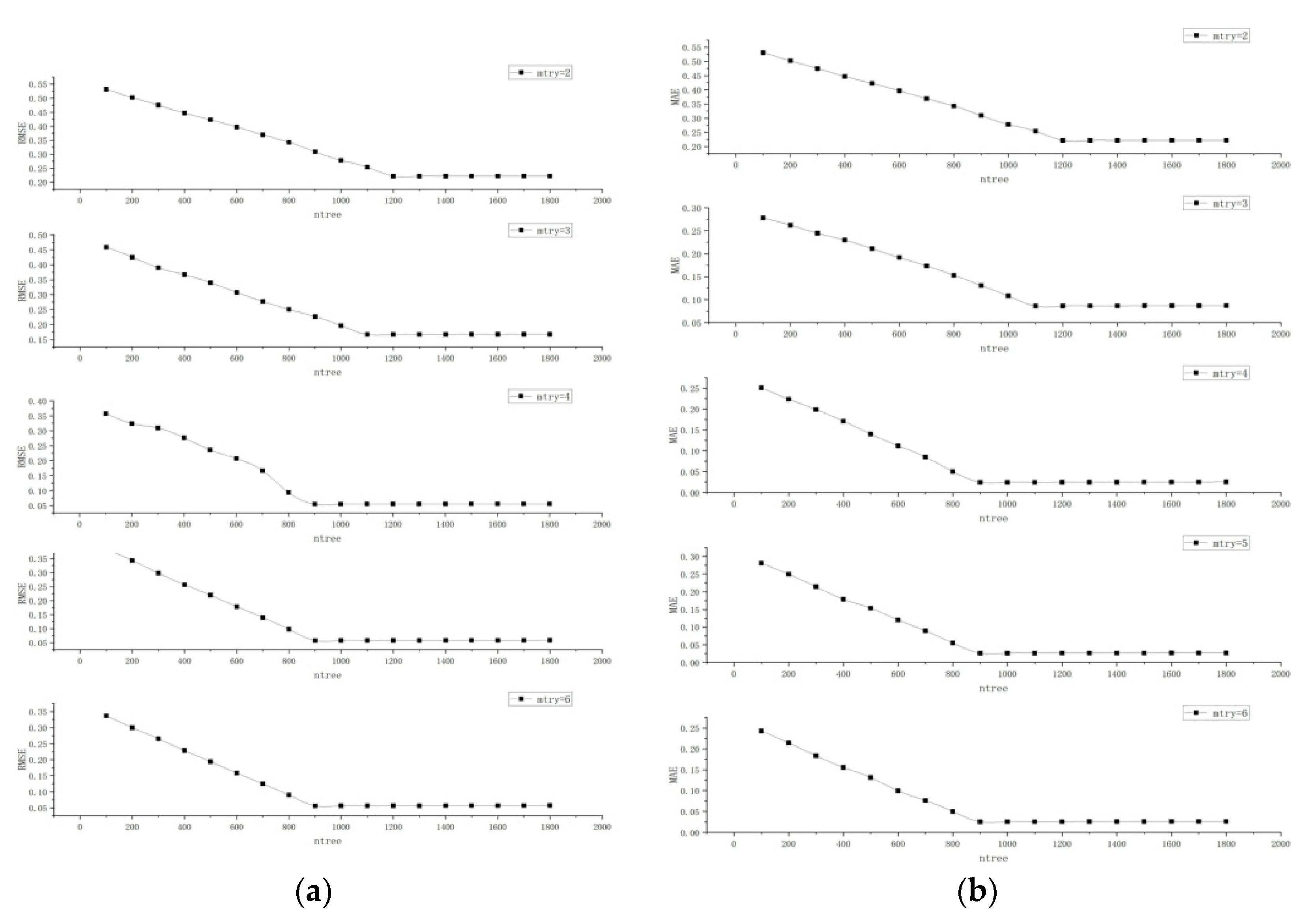
The parameters of the random forest regression model were iteratively optimized using the particle swarm algorithm, which had two main parameters: the number of decision trees (nTree) and the number of variables (mtry) randomly extracted from the nodes of the decision tree. To improve the accuracy of the random forest regression calculation by continuous iterative optimization, the RMSE and MAE were selected as the main factors. The iterative optimization of nTree and mtry was performed using MATLAB as a processing platform. Overall, the RMSE and MAE decreased as the number of decision trees (nTree) and the number of randomly extracted variables (mtry) at the nodes of the decision tree increased. The model error stabilized when both nTree and mtry increased to a certain extent.
According to the analysis in Figure 2, when the number of decision trees was 1200 with mtry = 2, the RMSE was 0.2215, and the MAE was 0.149. When the number of decision trees was 1100 with mtry = 3, the RMSE was 0.1672, and the MAE was 0.0862. When the number of decision trees was 900 after mtry > 3, the RMSE and MAE basically tended to stabilize: the RMSE was stable at about 0.055, and the MAE was stable at about 0.024. Increasing the nTree and mtry did not cause the model accuracy to continue to rise, so an nTree of 900 and an mtry of 4 were determined to be the parameters for the random forest regression model using the MATLAB regression learner.
3.2. Model Accuracy Analysis
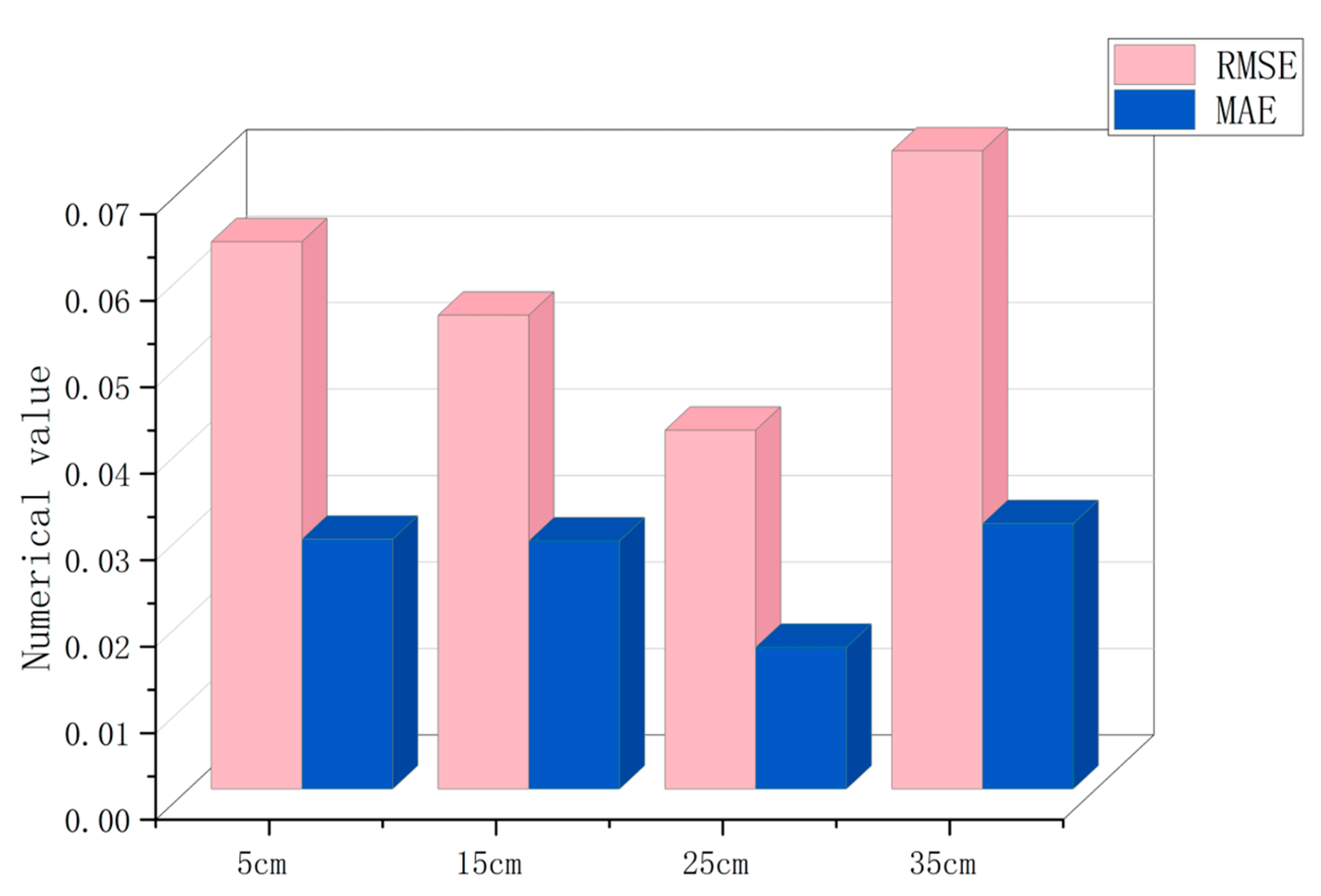
By fitting and testing the random forest regression model with the optimal parameters selected by the particle swarm optimization algorithm, considering the practical significance of forestry operation and management, the we analyzed the accuracy of the 5, 15, 25, and 35 cm diameter scale models. The results are shown in Table 3 and Figure 3. The four models all had satisfactory fitting effects (). Among them, the 25 cm model had the highest value, the lowest RMSE, and the best fitting effect. There was little difference between the 35 and 25 cm scale models, but the RMSE and MAE were the largest. The increase may have been due to a too small sample size. The value of the 5 cm model was the lowest: its MAE was the lowest and its average absolute error of model fitting was the smallest. Much of the accuracy of the 15 cm model was at the equilibrium level among the four models.
4. Discussion
4.1. Effect of Environmental Factors on Forest Density
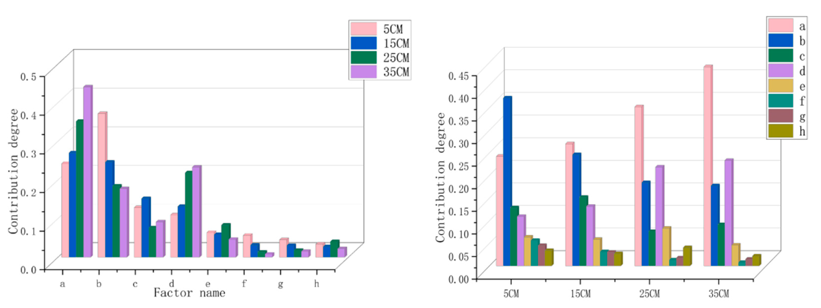
The contribution rates of different factors were analyzed. As shown in Table 4 and Figure 4, the average temperature factor was the largest in the 15, 25, and 35 cm models, and its contribution gradually increased with tree growth, indicating that the average temperature was the main factor restricting density. The same conclusion was reached in the study of tree radial growth [36]. The contribution rate of forest water consumption and soil thickness gradually decreased with continued growth, which may have been due to the fact that environmental factors were basically stable, and the forest water consumption and soil thickness constraints on tree density gradually decreased. In some studies of the impact of water resources on tree growth, it was also proposed that water resources are an important factor and vary depending on the different life stages of tree growth [37,38]. The contribution rate of dominant tree species factors increased with growth, which showed that different species restricted density and that the growth characteristics of different tree species led to the intensification of competition [39,40,41,42]. For soil type, slope, slope direction, and slope position, the contribution degree decreased with fluctuations in tree growth. These factors belong to long-term fixed factors, which do not increase greatly under normal circumstances, and the ability to restrict density gradually decreased as trees grew [43].
4.2. Effect of Environmental Factors on Forest Density
The independent variable contribution rates of the four models were analyzed, as shown in Figure 4 and Table 3. In the overall model, they were positively correlated; the average temperature showed the highest correlation (44.04%), and the slope showed the lowest (0.76%). In the 5 cm diameter class, the contribution rate of its main factors was analyzed. Forest water consumption (37.15%) > the contribution rate of average temperature (24.22%) > soil thickness (12.85%) > dominant tree species (10.92%), which showed that the forest was more sensitive to the environmental factors that directly affected its growth during the young tree period. These three kinds of habitat factors directly affected the tree density [44]. In the 15 cm diameter class, the average temperature (26.99%) > forest water consumption (24.61%) > soil thickness (15.17%) > dominant tree species (13.15%). It can be seen that the contribution rate of average temperature and forest water consumption decreased, and the contribution rate of soil thickness and dominant tree species increased. This may be due to the fact that the trees were basically mature (DBH reached 15 cm). Soil nutrient absorption and specific tree species had a greater impact on forest density [45]. In the 25 and 35 cm diameter class, in addition to average temperature and forest water consumption, the contribution rate of the dominant tree species increased to second place, which showed that as trees grew, the contribution rate of the dominant species to tree density increased, and the differences between different species became more pronounced [46,47].
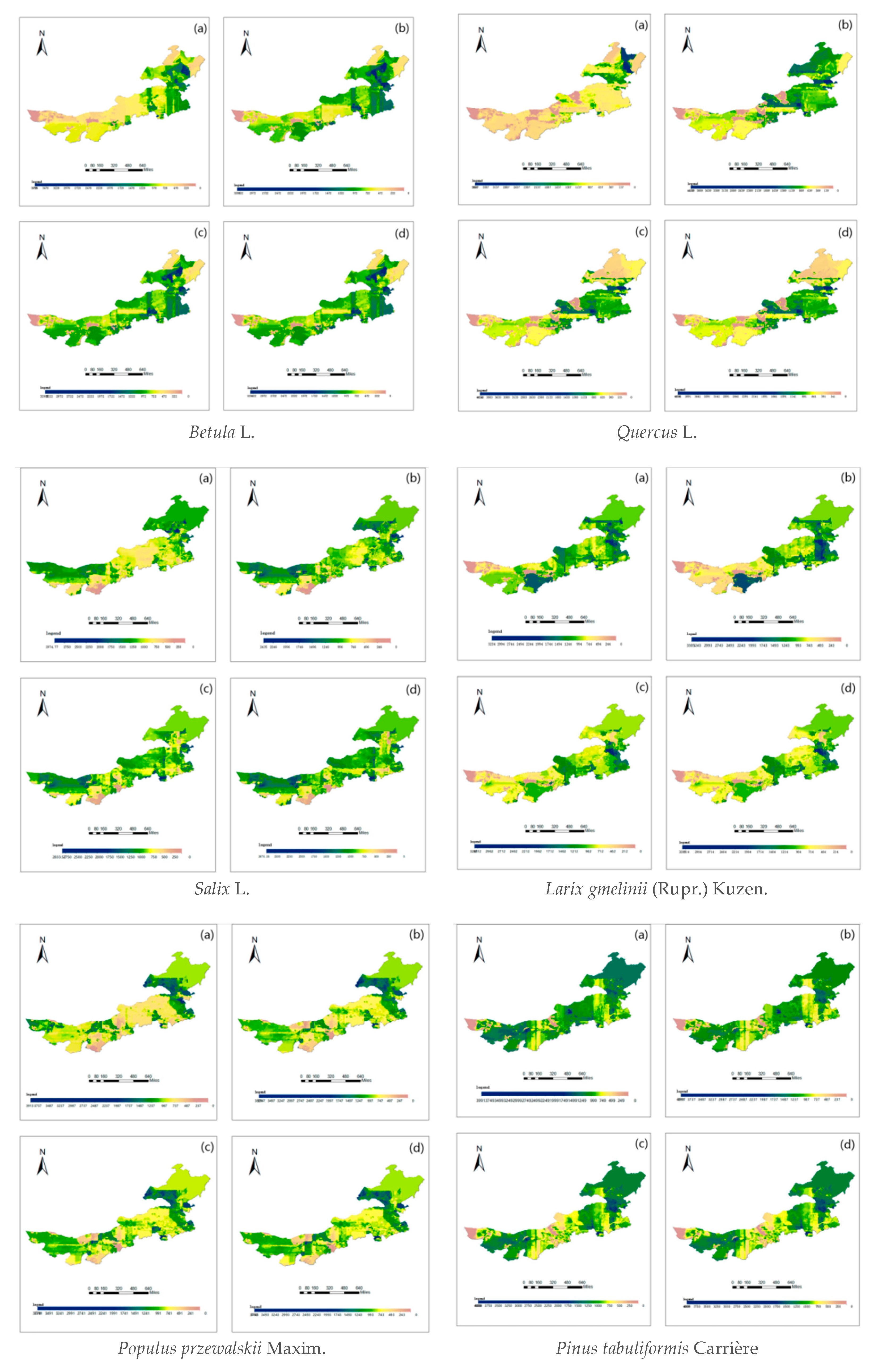
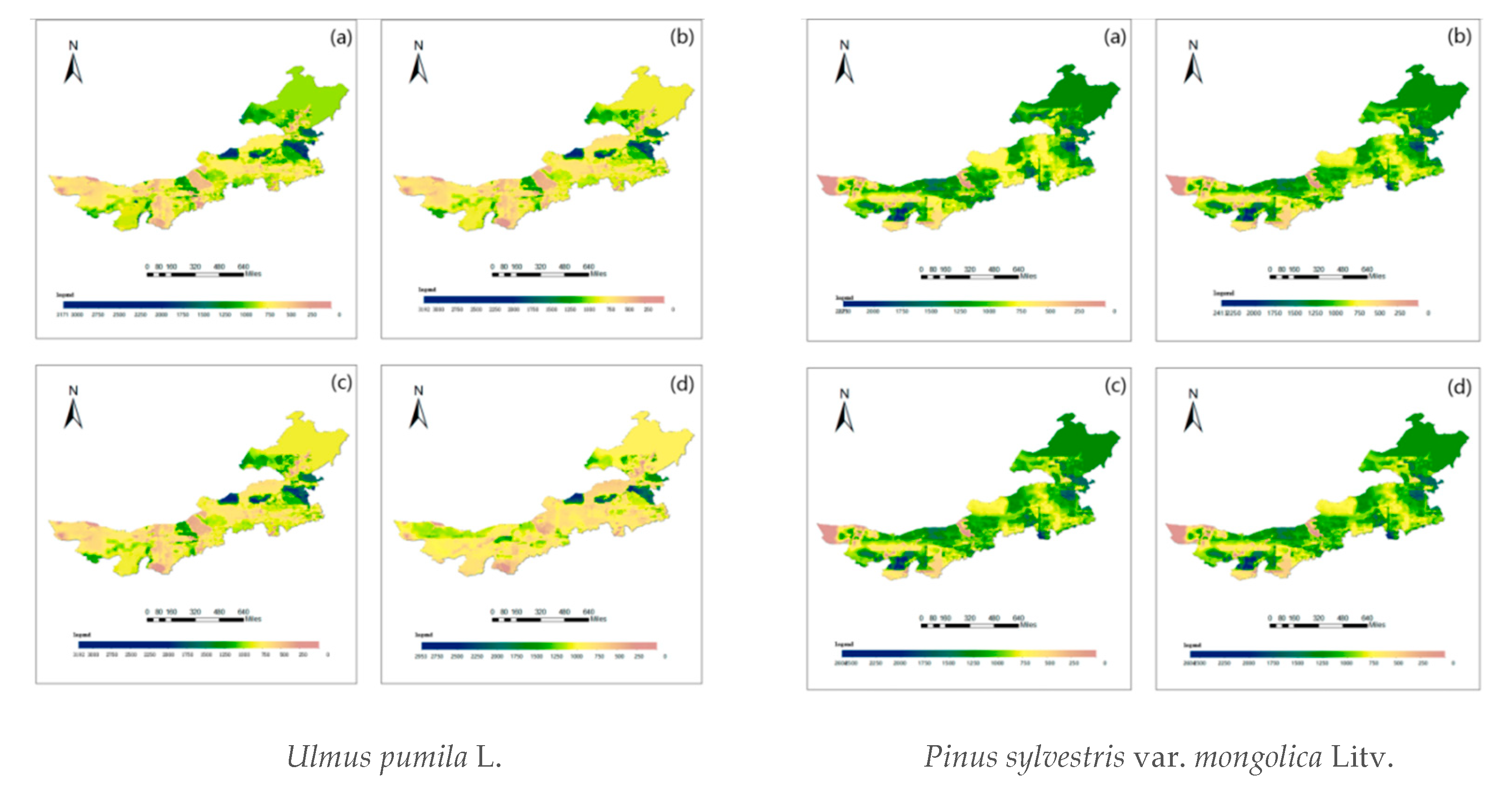
4.3. Raster Plot of Diameter Order Density Distribution of Various Tree Species in Inner Mongolia
Of all the forest resource data of the Inner Mongolia Autonomous Region used in this paper, aside from actual land use, only terrain, soil, and meteorological factors according to geographical coordinates were read. Using the main species—Larix gmelinii (Rupr.) Kuzen., Pinus sylvestris var. mongolica Litv., Pinus tabuliformis Carrière, Quercus L., Betula L., Ulmus pumila L., Populus przewalskii Maxim., and Salix L.—the stand density values of 5, 15, 25, and 35 cm diameter trees in each plot were calculated. Vector point data were processed by Kriging interpolation to form a grid map of the diameter class density distribution, as shown in the Figure 5 (considering that some readers may be color blind, all the graphics in this paper were made using the visolv software to address red and green recognition obstacles).
Map (a) refers to the initial planting of the seedlings of the corresponding tree species, and (b) shows young forests. Maps (c) and (d) depict mature forests. According to these grid data maps, the forest density in Inner Mongolia is regulated by tree species and diameter steps, which can be used as references for forest management by the Inner Mongolia Forest Department. This finding has strong practical significance for considering new afforestation, felling control, forest management, and failed afforestation sites [48,49,50].
5. Conclusions
Based on the 2018 forest resource data of the Inner Mongolia Autonomous Region, we selected multiple types of environmental factors as independent variables to explore the dominant factors affecting tree density. A particle swarm optimization algorithm was used to optimize the number of nTree values of random forest decision trees and the number of mtry values of variables randomly selected from decision tree nodes. Model fitting was carried out using MATLAB software. The fitting effect was adequate, and the determination coefficients were > 0.60. The model explains how environmental factors affect stand density, with analysis of the relevant factors affecting tree density and exploration of the changed law of tree density. The forest density of Inner Mongolia was calculated using this model, and the grid data of the diameter step density distribution of various tree species were formed by Kriging interpolation; these results have practical significance for forest management in the Inner Mongolia Autonomous Region. There is still room for the further optimization of the grid data for use in practical applications.
Author Contributions
Formal analysis, C.C. and Z.F.; Investigation, Z.L.; Methodology, C.C. and Z.F.; Project administration, Z.F.; Resources, Z.F.; Software, C.C.; Supervision, Z.F.; Validation, C.C. and Z.L.; Visualization, Z.L.; Writing—original draft, C.C.; Writing—review and editing, Z.F. All authors have read and agreed to the published version of the manuscript.
Funding
This study was supported by the National Natural Science Foundation of China. The National Natural Science Foundation number is U1710123.
Data Availability Statement
The steam and dispersion data of forest water consumption data used to support the findings of this study have been deposited in the “PML_V2 global evapotranspiration and gross primary production” repository (doi:10.11888/Geogra.tpdc.270251). The average temperature data used to support the findings of this study have been deposited in the “A combined Terra and Aqua MODIS land surface temperature and meteorological station data product for China (2003–2017)” repository (doi:10.5281/zenodo.3528024). The forest resource data in Inner Mongolia data used to support the findings of this study were supplied by the National Forest Resource Smart Management Platform under license and thus cannot be made freely available. Requests for access to these data should be made to the National Forestry and Prairie Administration, No.18 Pingli East Street, Dongcheng District, Beijing Postal Code: 100714.
Acknowledgments
This study was supported by the the National Natural Science Foundation of China (U1710123).
Conflicts of Interest
The authors declare no conflict of interest.
References
- Evans, J. Plantation Forestry in the Tropics: Tree Planting for Industrial, Social, Environmental, and Agroforestry Purposes; Clarendon Press, Oxford University Press: Oxford, UK, 1992. [Google Scholar]
- Hans, M.; Xiao, C.; He, M. Afforestation is Based on Community and Ecology. In Principles of Silvicultur; China Forestry Press: Beijing, China, 1986; Volume I. [Google Scholar]
- Zhang, J. Cultivation Technology of Fast-Growing and High-Yield Forest and Development Trend of Plantation in North China; China Forestry Industry: Beijing, China, 2004; Volume 5, p. 2. [Google Scholar]
- Li, M.; Li, C.; Xu, Z.; Li, X.; Sun, Y. Natural Rarefaction Model of Larch Leaf Tree Artificial Forest and Preparation of A Growth Process Table; Forest Investigation Design: Harbin, China, 1995; pp. 30–33. [Google Scholar]
- Webb, C.O.; Gilbert, G.S.; Donoghue, M.J. Phylodiversity-Dependent Seedling Mortality, Size Structure, and Disease in a Bornean Rain Forest. Ecology 2006, 87, S123–S131. [Google Scholar] [CrossRef] [Green Version]
- Metz, M.R.; Sousa, W.P.; Valencia, R. Widespread density-dependent seedling mortality promotes species coexistence in a highly diverse Amazonian rain forest. Ecology 2010, 91, 3675–3685. [Google Scholar] [CrossRef] [PubMed]
- Qin, J.; Zhang, Z.; Geng, Y.; Zhang, C.; Song, Z.; Zhao, X. Variations of density-dependent seedling survival in a temperate forest. For. Ecol. Manag. 2020, 468, 118158. [Google Scholar] [CrossRef]
- Liu, X.; Liang, M.; Etienne, R.; Wang, Y.; Staehelin, C.; Yu, S. Experimental evidence for a phylogenetic Janzen-Connell effect in a subtropical forest. Ecol. Lett. 2011, 15, 111–118. [Google Scholar] [CrossRef]
- Ness, J.H.; Morales, M.A.; Kenison, E.; Leduc, E.; Leipzig-Scott, P.; Rollinson, E.; Swimm, B.J.; Von Allmen, D.R. Reciprocally beneficial interactions between introduced plants and ants are induced by the presence of a third introduced species. Oikos 2013, 122, 695–704. [Google Scholar] [CrossRef]
- Zhu, Y.; Comita, L.S.; Hubbell, S.P.; Ma, K. Conspecific and phylogenetic density-dependent survival differs across life stages in a tropical forest. J. Ecol. 2015, 103, 957–966. [Google Scholar] [CrossRef]
- Wu, C.; Hong, H.; Jiang, Z. Study on the regulation law of density in the process of self thinning of Chinese fir forest. J. Trop. Subtrop. Plants 2000, 8, 7. [Google Scholar]
- Zhen, T.S.; Tong, S.W.; Zhang, J. Study on density effect of Chinese fir stand. For. Sci. Res. 2002, 1, 66–75. [Google Scholar]
- Aiguo, D.; Zhang, J.; Shuzhen, T.; Jiang, B.; He, H.Y. Dynamics of diameter structure and its density effect in Chinese fir plantation stands. For. Sci. Res. 2004, 17, 7. [Google Scholar]
- Zhang, H.Q.; Hao, D.W.; He, Y.; Li, H.P. Mathematical models for optimal control strategies of artificial forest forest density. J. Northeast. For. Univ. 2006, 34, 24–158. [Google Scholar]
- Wu, S.; Zhu, Q.; Yu, X.; Xue, P.Z. calculation and analysis of reasonable stand density of main forested tree species in the loess region of Jinxi, China. Soil Soil Conserv. Study 2008, 1, 83–86. [Google Scholar]
- Franklin, O.; Moltchanova, E.; Kraxner, F.; Seidl, R.; Böttcher, H.; Rokityiansky, D.; Obersteiner, M. Large-Scale Forest Modeling: Deducing Stand Density from Inventory Data. Int. J. For. Res. 2012, 2012, 934974. [Google Scholar] [CrossRef] [Green Version]
- Uhl, E.; Biber, P.; Ulbricht, M.; Heym, M.; Horváth, T.; Lakatos, F.; Gál, J.; Steinacker, L.; Tonon, G.; Ventura, M.; et al. Analysing the effect of stand density and site conditions on structure and growth of oak species using Nelder trials along an environmental gradient: Experimental design, evaluation methods, and results. For. Ecosyst. 2015, 2, 243–261. [Google Scholar] [CrossRef] [Green Version]
- Barrio-Anta, M.; Balboa-Murias, M.Á.; Castedo-Dorado, F.; Diéguez-Aranda, U.; Álvarez-González, J.G. An ecoregional model for estimating volume, biomass and carbon pools in maritime pine stands in Galicia (northwestern Spain). For. Ecol. Manag. 2006, 223, 24–34. [Google Scholar] [CrossRef]
- Lasky, J.R.; Sun, I.F.; Su, S.H.; Chen, Z.S.; Keitt, T.H. Trait-mediated effects of environmental filtering on tree community dynamics. J. Ecol. 2013, 101, 722–733. [Google Scholar] [CrossRef]
- Wu, J.; Swenson, N.G.; Brown, C.; Zhang, C.; Yang, J.; Ci, X.; Li, J.; Sha, L.; Cao, M.; Lin, L. How does habitat filtering affect the detection of conspecific and phylogenetic density dependence? Ecology 2016, 97, 1182–1193. [Google Scholar] [CrossRef]
- Pu, X.; Jin, G. Conspecific and phylogenetic density-dependent survival differs across life stages in two temperate old-growth forests in Northeast China. For. Ecol. Manag. 2018, 424, 95–104. [Google Scholar] [CrossRef]
- Uriarte, M.; Muscarella, R.; Zimmerman, J.K. Environmental heterogeneity and biotic interactions mediate climate impacts on tropical forest regeneration. Glob. Chang. Biol. 2018, 24, e692–e704. [Google Scholar] [CrossRef]
- Johnson, D.J.; Condit, R.; Hubbell, S.P.; Comita, L.S. Abiotic niche partitioning and negative density dependence drive tree seedling survival in a tropical forest. Proc. R. Soc. B Biol. Sci. 2017, 284, 20172210. [Google Scholar] [CrossRef]
- Wang, J.; Cheng, X.; Peng, J. A weighted random forest model based on particle swarm optimization. J. Zhengzhou Univ. 2018, 50, 72–76. [Google Scholar]
- Oshiro, T.M.; Perez, P.S.; Baranauskas, J.A. How many trees in a random forest? In International Workshop on Machine Learning and Data Mining in Pattern Recognition; Springer: Berlin/Heidelberg, Germany, 2012; pp. 154–168. [Google Scholar]
- Wen, X. Research on Key Technologies and Methods of Forest Resources Class II Survey; Nanjing Forestry University: Nanjing, China, 2017. [Google Scholar]
- Zhang, Y. PML_V2 Global Evapotranspiration and Gross Primary Production (2002.07–2019.08). National Tibetan Plateau Data Center. Available online: https://data.tpdc.ac.cn/en/data/48c16a8d-d307-4973-abab-972e9449627c/ (accessed on 8 December 2021).
- Zhao, B.; Mao, K.B.; Cai, Y.L.; Shi, J.C.; Li, Z.L.; Qin, Z.H.; Meng, X.J.; Shen, X.Y.; Guo, Z.H. A combined Terra and Aqua MODIS land surface temperature and meteorological station data product for China from 2003 to 2017. Earth Syst. Sci. Data 2020, 12, 2555–2577. [Google Scholar] [CrossRef]
- Roberts, D.R.; Bahn, V.; Ciuti, S.; Boyce, M.S.; Elith, J.; Guillera-Arroita, G.; Hauenstein, S.; Lahoz-Monfort, J.J.; Schröder, B.; Thuiller, W.; et al. Cross-validation strategies for data with temporal, spatial, hierarchical, or phylogenetic structure. Ecography 2017, 40, 913–929. [Google Scholar] [CrossRef]
- Cao, Z. Research on Optimization of Stochastic Forest Algorithm. Ph.D. Thesis, Capital University of Economics and Trade, Beijing, China, 2014. [Google Scholar]
- Pal, M. Random forest classifier for remote sensing classification. Int. J. Remote Sens. 2005, 26, 217–222. [Google Scholar] [CrossRef]
- Probst, P.; Boulesteix, A.L. To tune or not to tune the number of trees in random forest. J. Mach. Learn. Res. 2017, 18, 6673–6690. [Google Scholar]
- Boulesteix, A.L.; Janitza, S.; Kruppa, J.; König, I.R. Overview of random forest methodology and practical guidance with emphasis on computational biology and bioinformatics. Wiley Interdiscip. Rev. Data Min. Knowl. Discov. 2012, 2, 493–507. [Google Scholar] [CrossRef] [Green Version]
- Afanador, N.L.; Smolinska, A.; Tran, T.N.; Blanchet, L. Unsupervised random forest: A tutorial with case studies. J. Chemom. 2016, 30, 232–241. [Google Scholar] [CrossRef]
- Shi, Y.; Eberhart, R.C. Empirical study of particle swarm optimization. In Proceedings of the 1999 Congress on Evolutionary Computation-CEC99 (Cat. No. 99TH8406), Washington, DC, USA, 6–9 July 1999; Volume 3, pp. 1945–1950. [Google Scholar]
- Huang, J.; Tardif, J.C.; Bergeron, Y.; Denneler, B.; Berninger, F.; Girardin, M.P. Radial growth response of four dominant boreal tree species to climate along a latitudinal gradient in the eastern Canadian boreal forest. Glob. Change Biol. 2010, 16, 711–731. [Google Scholar] [CrossRef]
- Lv, S.; Wang, X. Climate response and winter precipitation reconstruction of Pinus sylvestris var. mongolica growth rings in Ali River in the north of Daxing’an Mountains. J. Northeast. Norm. Univ. 2014, 46, 110–116. [Google Scholar]
- Xi, B.; Di, N.; Jinqiang, L.; Li, D.; Cao, Z. Characteristics and mechanism of deep soil water absorption and utilization by trees: Enlightenment to plantation cultivation. J. Plant Ecol. 2018, 42, 21. [Google Scholar]
- Webb, C.O.; Peart, D.R. Seedling density dependence promotes coexistence of bornean rain forest trees. Ecology 1999, 80, 2006–2017. [Google Scholar] [CrossRef]
- Wills, C.; Condit, R.; Foster, R.B.; Hubbell, S.P. Strong density- and diversity-related effects help to maintain tree species diversity in a neotropicalforest. Proc. Natl. Acad. Sci. USA 1997, 94, 1252–1257. [Google Scholar] [CrossRef] [PubMed] [Green Version]
- Schupp, E.W. The Janzen-Connell Model for Tropical Tree Diversity: Population Implications and the Importance of Spatial Scale. Am. Nat. 1992, 140, 526–530. [Google Scholar] [CrossRef] [PubMed]
- Clark, D.A.; Clark, D.B. Spacing dynamics of a tropical rain-forest tree—Evaluation of the janzen-connell model. Am. Nat. 1984, 124, 769–788. [Google Scholar] [CrossRef]
- Zhu, Y. Study on Tree Death and Species Coexistence in Typical Broad-Leaved Korean Pine Forest. Ph.D. Thesis, Northeast Forestry University, Harbin, China, 2018. [Google Scholar]
- Yang, B. Response of Robinia Pseudoacacia Seedlings to Water Stress: Based on the Distribution and Dynamics of Growth, Physiology and Non Structural Carbon Diss; Northwest University of Agriculture and Forestry Science and Technology: Xianyang, China, 2019; pp. 21–23. [Google Scholar]
- Ying, H.; Ying, Y.; Yu, L.Z.; Zhang, X.B.; Yao, B. Research progress on the effects of soil moisture and nutrients on the growth dynamics and turnover of fine roots of trees. J. Northwest For. Univ. 2010, 25, 7. [Google Scholar]
- Luo, M.; Chen, S. Study on intraspecific and interspecific competition of Larix olgensis with different age groups. J. Beijing For. Univ. 2018, 40, 33–44. [Google Scholar] [CrossRef]
- Wei, X. Study on the Coupling Relationship between Typical Plantation Structure and Soil and Water Conservation Function in Loess Region of Western Shanxi. Ph.D. Thesis, Beijing Forestry University, Beijing, China, 2018. [Google Scholar]
- Hong, L.; Lei, X.; Li, Y. Overall growth model of Mongolian oak forest and its application. For. Sci. Res. 2012, 25, 201–206. [Google Scholar] [CrossRef]
- Stankova, T.V.; Shibuya, M. Stand Density Control Diagrams for Scots pine and Austrian black pine plantations in Bulgaria. New For. 2007, 34, 123–141. [Google Scholar] [CrossRef]
- Yin, T.; Han, F.; Chi, J.; Wu, B. Compilation and application of stand density control chart. China For. Sci. 1978, 3, 1–11. [Google Scholar]
Figure 1.
Diagram showing the distribution of the main tree species in Inner Mongolia, where the different colors represent different tree species.
Figure 1.
Diagram showing the distribution of the main tree species in Inner Mongolia, where the different colors represent different tree species.

Figure 2.
The particle swarm algorithm iteratively optimizes the graph, where (a) is the RMSE change and (b) is the MAE change.
Figure 2.
The particle swarm algorithm iteratively optimizes the graph, where (a) is the RMSE change and (b) is the MAE change.

Figure 3.
Error range diagram of random forest model with different diameter orders in which pink represents RMSE and blue represents MAE.
Figure 3.
Error range diagram of random forest model with different diameter orders in which pink represents RMSE and blue represents MAE.

Figure 4.
The contribution rate of different independent factors in the random forest model: a is average temperature, b is forest water consumption, c is soil thickness, d is dominant tree species, e is soil type, f is slope, g is slope direction, and h is slope position.
Figure 4.
The contribution rate of different independent factors in the random forest model: a is average temperature, b is forest water consumption, c is soil thickness, d is dominant tree species, e is soil type, f is slope, g is slope direction, and h is slope position.

Figure 5.
Raster plot of diameter order density distribution of various tree species in inner mongolia.
Figure 5.
Raster plot of diameter order density distribution of various tree species in inner mongolia.


Table 1.
Schematic diagram of forest density distribution range in Inner Mongolia, in which N represents forest density. Unit: plant/ha.
Table 1.
Schematic diagram of forest density distribution range in Inner Mongolia, in which N represents forest density. Unit: plant/ha.
| Diameter Class | Total Number of Forest Subclasses | N ≤ 500 | 500 < N ≤ 1500 | 1500 < N ≤ 2500 | N > 2500 |
|---|---|---|---|---|---|
| 5 | 445,501 | 27,100 | 346,029 | 65,397 | 6975 |
| 15 | 509,709 | 53,531 | 364,313 | 74,249 | 17,616 |
| 25 | 47,207 | 10,735 | 29,165 | 3576 | 3731 |
| 35 | 5287 | 1492 | 3507 | 278 | 10 |
Table 2.
Summary table of main factors involved in model building.
| Data Name | Data Type | Time | Data Resolution | Data Sources | Variable Type |
|---|---|---|---|---|---|
| Stand density | Continuous variable | 2018 | Minor class size | Intelligent management platform for forest resources in China | Response variable |
| Soil thickness | Continuous variable | 2018 | Minor class size | Intelligent management platform for forest resources in China | Input variables |
| Dominant tree species | Categorical variable | 2018 | Minor class size | Intelligent management platform for forest resources in China | Categorical variable |
| Soil type | Categorical variable | 2018 | Minor class size | Intelligent management platform for forest resources in China | Categorical variable |
| Slope | Categorical variable | 2018 | Minor class size | Intelligent management platform for forest resources in China | Categorical variable |
| Slope direction | Categorical variable | 2018 | Minor class size | Intelligent management platform for forest resources in China | Categorical variable |
| Slope position | Categorical variable | 2018 | Minor class size | Intelligent management platform for forest resources in China | Categorical variable |
| Average temperature | Continuous variable | 2008–2017 mean value | 0.05° | National Science and technology data center for Qinghai, Tibet Plateau | Input variables |
| Forest water consumption | Continuous variable | 2008–2017, mean value | 5600 m | National Science and technology data center for Qinghai, Tibet Plateau | Input variables |
Table 3.
Table of sample quantity and accuracy of random forest model construction of different diameter classes.
Table 3.
Table of sample quantity and accuracy of random forest model construction of different diameter classes.
| Model | Total Number of Samples | RMSE | MAE | |
|---|---|---|---|---|
| 5 cm diameter scale model | 445,501 | 0.0633 | 0.0157 | 0.6159 |
| 15 cm diameter scale model | 509,709 | 0.0548 | 0.0287 | 0.7097 |
| 25 cm diameter scale model | 47,207 | 0.0415 | 0.0164 | 0.7512 |
| 35 cm diameter scale model | 5287 | 0.0738 | 0.0307 | 0.7299 |
Table 4.
Contribution rates of different independent variables in the random forest model.
| Factor Name | 5 cm | 15 cm | 25 cm | 35 cm |
|---|---|---|---|---|
| Average temperature | 24.22% | 26.99% | 35.17% | 44.04% |
| Forest water consumption | 37.15% | 24.61% | 18.42% | 17.73% |
| Soil thickness | 12.85% | 15.17% | 7.60% | 9.12% |
| Dominant tree species | 10.92% | 13.15% | 21.85% | 23.31% |
| Soil type | 6.36% | 5.86% | 8.31% | 4.59% |
| Slope | 5.63% | 3.13% | 1.32% | 0.76% |
| Slope direction | 4.50% | 3.01% | 1.75% | 1.47% |
| Slope position | 3.40% | 2.71% | 4.04% | 2.18% |
Publisher’s Note: MDPI stays neutral with regard to jurisdictional claims in published maps and institutional affiliations. |
© 2022 by the authors. Licensee MDPI, Basel, Switzerland. This article is an open access article distributed under the terms and conditions of the Creative Commons Attribution (CC BY) license (https://creativecommons.org/licenses/by/4.0/).
Share and Cite
MDPI and ACS Style
Chang, C.; Feng, Z.; Liu, Z. A Study of the Distribution of Forest Density in Inner Mongolia Based on Environmental Factors. Forests 2022, 13, 313. https://0-doi-org.brum.beds.ac.uk/10.3390/f13020313
AMA Style
Chang C, Feng Z, Liu Z. A Study of the Distribution of Forest Density in Inner Mongolia Based on Environmental Factors. Forests. 2022; 13(2):313. https://0-doi-org.brum.beds.ac.uk/10.3390/f13020313
Chicago/Turabian StyleChang, Chen, Zhongke Feng, and Ziye Liu. 2022. "A Study of the Distribution of Forest Density in Inner Mongolia Based on Environmental Factors" Forests 13, no. 2: 313. https://0-doi-org.brum.beds.ac.uk/10.3390/f13020313
Note that from the first issue of 2016, this journal uses article numbers instead of page numbers. See further details here.