Article

Assessment of Air Quality and Meteorological Changes Induced by Future Vegetation in Madrid

1
Department of Chemical and Environmental Engineering, ETSII—Universidad Politécnica de Madrid (UPM), 28040 Madrid, Spain
2
ARIANET, 20159 Milán, Italy
3
Research Centre for Forestry and Wood, Council for Agricultural Research and Economics (CREA), 00184 Rome, Italy
4
Institute of BioEconomy, National Research Council of Italy (CNR), 00185 Rome, Italy
5
Ayuntamiento de Madrid, 28014 Madrid, Spain
6
Laboratory of Atmospheric Pollution, Italian National Agency for New Technologies, Energy and Sustainable Economic Development—ENEA, 40129 Bologna, Italy
*
Author to whom correspondence should be addressed.
Submission received: 29 March 2022 / Revised: 20 April 2022 / Accepted: 27 April 2022 / Published: 29 April 2022

Abstract

:
Nature-based solutions and green urban infrastructures are becoming common measures in local air quality and climate strategies. However, there is a lack of analytical frameworks to anticipate the effect of such interventions on urban meteorology and air quality at a city scale. We present a modelling methodology that relies on the weather research and forecasting model (WRF) with the building effect parameterization (BEP) and the community multiscale air quality (CMAQ) model and apply it to assess envisaged plans involving vegetation in the Madrid (Spain) region. The study, developed within the VEGGAP Life project, includes the development of two detailed vegetation scenarios making use of Madrid’s municipality tree inventory (current situation) and future vegetation-related interventions. An annual simulation was performed for both scenarios (considering constant anthropogenic emissions) to identify (i) variations in surface temperature and the reasons for such changes, and (ii) implications on air-quality standards according to EU legislation for the main pollutants (PM10, PM2.5, NO2 and O3). Our results suggest that vegetation may have significant effects on urban meteorology due to changes induced in relevant surface properties such as albedo, roughness length or emissivity. We found a net-heating effect of around +0.18 °C when trees are introduced in dry, scarcely vegetated surfaces in the city outskirts. In turn, this enhances the planetary boundary layer height (PBLH), which brings about reductions in ambient concentrations of relevant pollutants such as NO2 (in the range of 0.5–0.8 µg m−3 for the annual mean, and 2–4 µg m−3 for the 19th highest 1 h value). Conversely, planting new trees in consolidated urban areas causes a cooling effect (up to −0.15 °C as an annual mean) that may slightly increase concentration levels due to less-effective vertical mixing and wind-speed reduction caused by increased roughness. This highlights the need to combine nature-based solutions with emission-reduction measures in Madrid.

Graphical Abstract

1. Introduction

Climate change impacts are expected to increase in severity and frequency in the coming decades [1,2,3]. In this context, nature-based solutions (NBS) may contribute to reducing risk related to climate change and restoring and protecting ecosystems, while providing multiple additional benefits (environmental, social and economic) [4,5].
According to [6], the concept of NBS lies on the boundaries between science and policy. Even though these solutions have not yet been widely adopted in policy, planning, and governance so far [7], in recent years they have been becoming increasingly popular in urban strategies to deal with the environmental dysfunctions of densely populated areas that have negative health effects on urban populations [8,9].
The role of nature supporting the economy as well as the livelihood of citizens has been widely described in the scientific literature. According to [10], several main NBS actions are recommended to be taken forward: urban regeneration [11], coastal resilience [12,13], multifunctional nature-based watershed management and ecosystem restoration [14], increasing the sustainable use of matter and energy as well as carbon sequestration [15], fostering outdoor activities for mental and physical health [16,17], enhancing the insurance value of ecosystems and improving wellbeing in urban areas [18,19].
As to this last point, the introduction of vegetation in cities has associated benefits regarding climate-change mitigation, such as an increase in street shadows or a decrease in the heat-island effect, that are of essential importance for the health and living comfort of city dwellers [20,21]. Vegetation in cities has also been described as a way to mitigate pollution thanks to enhanced wet- and dry-deposition processes [22,23,24]. However, vegetation is also a source of emissions for some substances, such as pollen and ozone, and particulate matter precursors that can affect negatively people’s health [25,26,27]. These negative impacts of urban ecosystems on urban dwellers are defined as ecosystem disservices (EDS) [28].
Vegetation is the main source of atmospheric volatile organic compounds (VOCs), accounting for about 90% of the total emissions worldwide [29]. Biogenic VOC (BVOCs), dominated by isoprene and monoterpenes, are an important atmospheric constituent affecting both the gas phase and heterogeneous chemistry of the troposphere [30], as well as being important precursors for the formation of ozone and secondary organic aerosols (SOA) [31,32,33], which may exacerbate respiratory conditions such as rhinitis and asthma [34,35].
However, the effect of vegetation on local air quality is very complex and depends on many more factors than just emissions. Urban vegetation modifies the local meteorology by affecting air temperature and relative humidity [36,37,38], altering the wind direction and wind speed due to changes in terrain roughness [39,40,41], and changing the thermal properties of the surface, such as surface albedo, surface humidity, etc. [42]. All these factors modify the boundary layer height (BLH) that controls the vertical mixing of urban pollutants and, therefore, their corresponding concentration levels [43].
Therefore, it is necessary to develop assessment tools that allow a consistent analysis of the air-quality effects associated with the implementation of green infrastructures in the design of plans and measures involving vegetation in urban areas.
To date, there are few studies in the scientific literature that delve into the impact of NBS on air quality, and most of them address the aerodynamic and deposition effects of vegetation on street/neighborhood ventilation and on pollutant concentration by means of computational fluid dynamic (CFD) simulations [44,45,46,47,48]. While these studies provide valuable information on the impact of vegetation at a microscale, they are not able to describe the complex chemical and physical atmospheric processes that account for the formation of secondary pollutants. The effects of city-wide NBS transcend the microscale level, so they must be studied from a broader, mesoscale approach [49]. The work presented here, developed within the VEG-GAP Life project (https://www.lifeveggap.eu, accessed 20 april 2022), aims at consistently quantifying the overall effects of future vegetation-related interventions in or around the city of Madrid on local meteorology and air quality, including secondary pollutants, through mesoscale simulations.

2. Materials and Methods

2.1. Description of the Model System

This study relies on a state-of-the-science modelling system that includes three main components: (i) a meteorological model, (ii) an emission model and (iii) a chemical-transport model. To analyze the impact of vegetation on meteorology and to provide the relevant inputs for the chemical-transport model, we applied WRFv4.1.2 (weather research and forecasting) [50], coupled with the building energy parametrization (BEP) [51]. Physical options and parametrizations are shown in Table 1. They were selected according to previous sensitivity analyses specifically made for this modelling domain [52,53]. Of note, we selected the PBL scheme that has a better compatibility with BEP and it is thus recommended by the developers of this urban parameterization [51].
We performed a comprehensive statistical assessment of WRF outputs for the complete year 2015 (baseline scenario for the VEGGAP project). As summarized in Tables S1 and S2 in the Supplementary Material, we found a satisfactory model performance for a mesoscale model, suggesting that our results are reliable enough to support the analysis proposed.
Anthropogenic emissions were processed through SMOKEv3.6.5 (Sparse Matrix Operator Kernel System) [54], specifically adapted for the Iberian Peninsula [55,56]. The estimation of emissions from the vegetation relies on PSEM (plant-specific emission model) [57] that includes specific basal emission factors for a wide range of tree species that are modified according to concurrent temperature, solar radiation and seasonality for each meteorological scenario. This allows a consistent representation of biogenic VOCs and meteorological information used to feed the chemical-transport model CMAQv5.3.2 [58,59]. Through a nested domain approach [60] CMAQ provides a consistent representation of physical transport and deposition phenomena, as well as chemical reactions in the atmosphere. In this study, they were represented by the carbon bond (CB6) chemical mechanism [61] and the aerosol module AERO6 [62]. This modelling approach allows a consistent estimation of all physical and chemical properties of atmosphere. Following the objectives of the VEG-GAP project, we focus the analysis on NO2, PM and O3, which are the most relevant pollutants in Madrid [63].

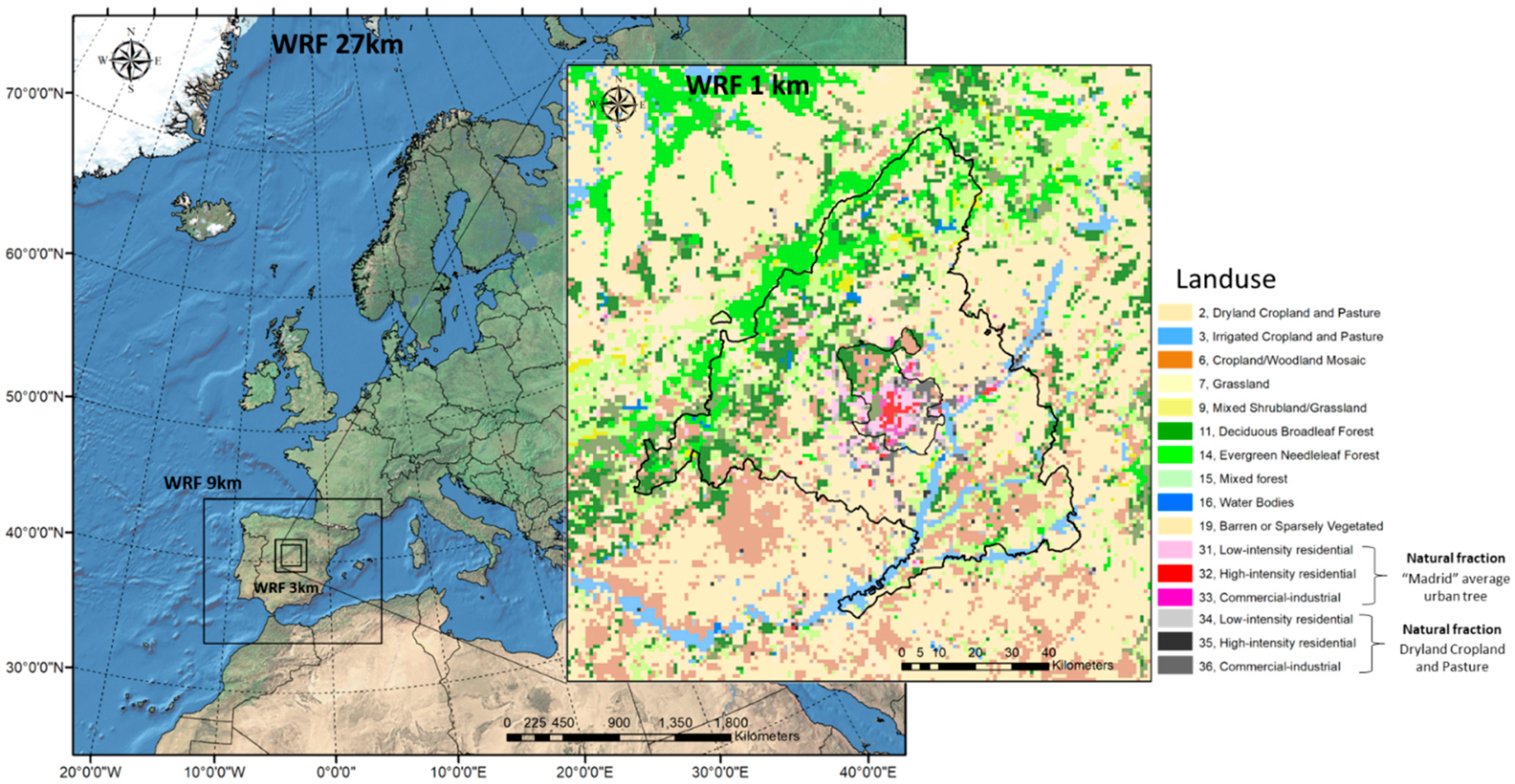
2.2. Modelling Domains

The nested modelling domains used in this study are shown in Figure 1. The mother domain (D1) covers the whole of Europe and Northern Africa with a spatial resolution of 27 × 27 km and provides dynamic boundary conditions for D2, which includes the Iberian Peninsula, with a spatial resolution of 9 × 9 km. D3, with a spatial resolution of 3 × 3 km, focuses on the central area of Spain; additionally, finally, the innermost modelling domain focuses on the Madrid Region, with a spatial resolution of 1 × 1 km. The results and discussion are based on the model outputs for this domain, which consists of 136 × 144 grid cells in the east—west direction and the north—south direction, respectively. As shown in Table S2 (Supplementary Material), the modelling domains used for WRF are slightly larger, to avoid boundary artifacts. The vertical structure is identical for all 4 modelling domains and it includes 38 layers entirely covering the troposphere. Of note, we include 18 layers within the first kilometer (the lower vertical level has a 7 m height) above the ground to allow a detailed representation of relevant atmospheric processes within the planetary boundary layer.
The temporal domain of our simulations covers the entire year 2015, so we can capture the effect of vegetation under a wide range of meteorological conditions and phenologies. In addition, this allows us to assess the impact of vegetation on air-quality standards according to the Air Quality Directive 2008/50/EC, such as annual limit values for NO2, PM10, PM2.5 and O3.

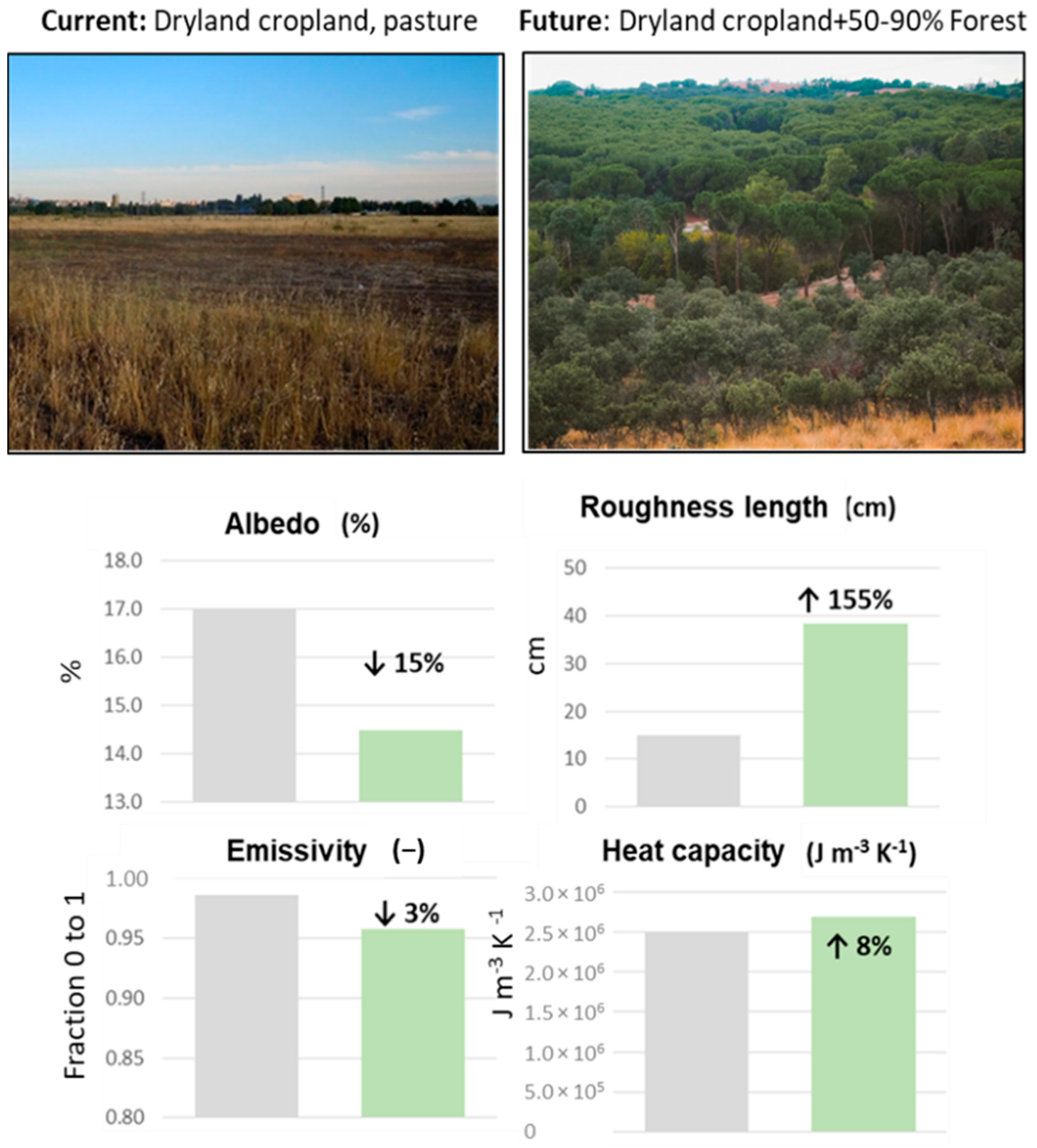
2.3. Vegetation Scenarios

We assessed the impact of vegetation-related interventions on meteorology and air quality through the comparison of two scenarios (both annual runs):
  • Baseline: intended to represent the current situation (year 2015);
  • Future: incorporates the vegetation associated to intended measures in the whole Madrid Region.
Surface properties in a mesoscale meteorological model, such as WRF, are represented by average biophysical properties of different land uses that govern the exchange of heat and momentum between the atmosphere and the ground. Current land uses were taken from the Corine land cover (CLC 2012) and mapped to USGS classes. The details of this procedure can be found elsewhere [53]. These include natural and urban classes, where built up areas are significant. In the second case, grid cells may include some vegetation too and their influence on such properties needs to be considered as well. The part of the modelling system that solves the interactions between the atmosphere and the ground depending on the land-use type (Figure 1) is the land-surface model (LSM), a particularly important feature for this study. We relied on the Noah land-surface model (LSM) [64], which has been identified as the best-performing option for our modelling domain in previous studies [52,53]. However, the Monin–Obukhov similarity theory (MOST) behind LSM in mesoscale models does not hold on urban areas, so the multilayer urban parameterization BEP was applied for our simulations in D4. This urban canopy parameterization considers 3 urban land use classes: ‘Low Intensity Residential’, LIR (31), ‘High Intensity Residential’, HIR (32) and ‘Commercial & Industrial’, C&I (33). The user of the standard model defines an average urban fraction, UF (ranging from 0 to 1), for each of these categories, representing the fraction of the surface covered by artificial materials (buildings, roads and sidewalks). In the present study, we assigned UF for each grid cell using the variable FRC_URB2D. The remaining area (1-UF) within urban grid cells is addressed as natural fraction and assigned the same physical properties (those of ‘Cropland/grassland mosaic’, default land-use type). Using a single land use to represent the non-urban fractions in built areas is a strong simplification, since important properties such as leaf area index (LAI), albedo, canopy height or roughness length may vary largely depending on the actual vegetation in different grid cells within the city.
In order to increase the flexibility of this modelling framework and to describe more realistically different interventions related to urban vegetation, we introduced some modifications in the code. Specifically, we added 6 new urban land uses (34 to 39) to allow the model to map the natural-fraction properties (that apply to 1-UF fraction of each grid cell) to 6 different natural-land uses that may be present in the city.

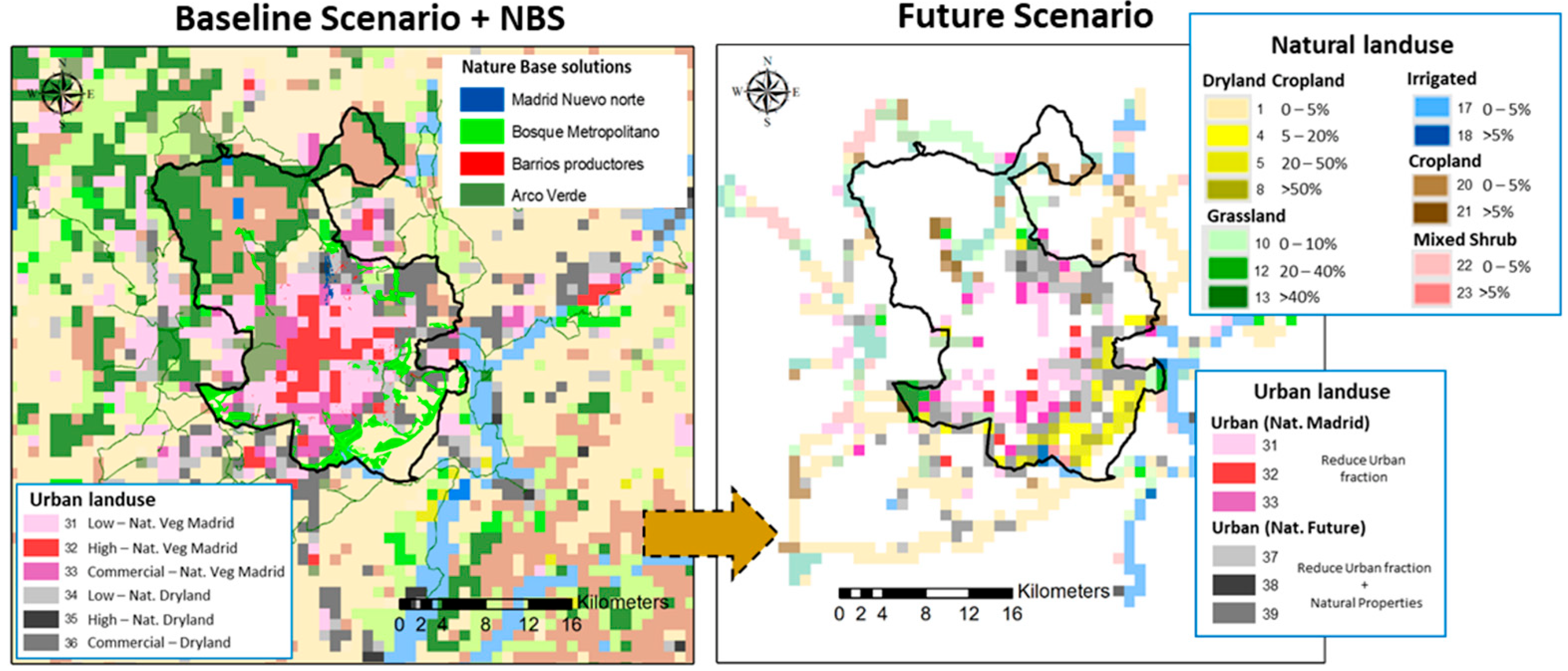
2.3.1. Baseline Scenario

This scenario includes 6 urban land-use types (31 and 34 for LIR, 32 and 35 for HIR and 33 and 36 for C&I). The difference between the different categories for a given urban morphology is the vegetation type present in the non-urban fraction. To represent this, we made use of Madrid’s municipality tree inventory, which includes detailed information for each tree in the city (location, species, height, etc.). We analyzed this high-resolution urban vegetation cover to define the ‘average urban tree’ in Madrid, which was assigned relevant properties according to the values provided by the Noah LSM. The ‘average urban tree’ in Madrid is 85% ‘Deciduous Broadleaf Forest’, 13% ‘Evergreen Needleleaf Forest’ and 2% ‘Evergreen Broadleaf Forest’. Weighted properties (Table S4) were assigned to the natural fraction of land uses 31, 32 and 33 according to these percentages. For the natural fraction of other urban categories (34, 35 and 36), the properties of the ‘Dryland, Cropland and Pasture’ land-use class were assigned (Table S4).

2.3.2. Future Scenario

We built a Future Scenario that intends to represent all the relevant interventions envisaged in urban plans and strategies for Madrid in the next decades (Figure 2). The 4 major naturalization measures included in this scenario are as follows:
  • ‘Arco verde’: linear plantations along drovers’ roads, trails and other rural paths to connect already existing periruban forests or green areas, a number or native species are considered.
  • ‘Barrios productores’: areas designated for the municipal network of urban vegetable gardens, considered as low-density shrub areas.
  • ‘Madrid Nuevo Norte’: a major urban development approved by the local and regional governments. It is intended to be a carbon-neutral mix of uses including new residential, business and green areas. Lacking more specific information, we have assumed that this green area will have the average characteristics (in term of species and density) of existing parks in Madrid.
  • ‘Bosque metropolitano’: The metropolitan forest is the most ambitious action of NBS projected for the coming years in the city of Madrid. It is framed on the air-quality and climate-change plans and the sustainability and urban green infrastructure strategies. This action aims to create a 75 km periurban green ring, which will connect existing parks, gardens and natural spaces and expand the urban green areas by more than 5000 hectares.
Since the project was in definition stage, the allocation and exact selection of tree species was not completely defined at the moment of performing our simulations; therefore, using the existing information as a base, we had to make some assumptions regarding trees and shrubs species and plantation density, according to the soil types, topography, etc., of each intervention area.
All combined, 724 grid cells were affected by vegetation changes in the Future Scenario. A total of 65% of them are non-urban land uses, mostly ‘Dryland Cropland and Pasture’ (42%) and ‘Grassland’ (13%), while the remaining 35% are urban areas. For the first group, each grid cell was re-classified into 4 new natural-land uses. Grid cells formerly not wooded were assigned to classes not present in our modelling domain. While all of them assume the average properties for new trees, they differ in the surface within the grid cell affected by reforestation (0%–5%, 5%–20%, 20%–50% and >50%, respectively). Physical properties (albedo, canopy height, roughness length, etc.) were computed as weighted averages using these percentages (Table S4). Figure 3 provides the example of a grid cell affected by the ‘Bosque metropolitano’.
As for urban grid cells where new vegetation is introduced (35%), we considered 2 different cases. For grid cells labelled as 31 (LIR), 32 (HIR) or 33 (C&I), urban classes that already contain trees, we simply reduced the urban fraction (UF), keeping vegetation properties unchanged. This is the case of 5% of urban grid cells affected by future interventions. For those urban land uses that do not contain trees (classes 34 (LIR), 35 (HIR) and 36 (C&I)), in addition to the corresponding change of the UF, the properties of the natural fraction (1-UF) were changed to match those of the vegetation being introduced. New land-use categories, 37, 38 and 39, were assigned to urban grid cells whose natural fraction was ‘Dryland Cropland and Pasture’ before the intervention, depending on the percentage of area affected by tree plantation. For simplicity, we assumed the average properties to be representative of ‘Bosque metropolitan,’ since it is the most important intervention (88% of the total area of future revegetation actions in Madrid). This corresponds to 90% ‘Dryland Cropland and Pasture’, 7% ‘Evergreen Needleleaf Forest’ and 3% ‘Deciduous Broadleaf Forest’.
While BVOC emissions were provided by PSEM (considering species-specific emission rates), using scenario-specific meteorology, we kept anthropogenic emission constant for both scenarios. Although this may be rather unrealistic for the Future Scenario, we assumed this experimental design to be able to isolate the specific impact of vegetation for a given level of emissions.

3. Results and Discussion

First, we present the impact of vegetation on urban meteorology, focusing on temperature, PBLH and wind speed as relevant variables for air quality [65,66]. Then, we summarize our findings regarding NO2, O3, PM10, and PM2.5 ambient concentration levels. We discuss the results averaged over the complete year as well as the winter (21 December to 21 March) and summer (21 June to 21 September) periods, to gain a better perspective on seasonal variability.

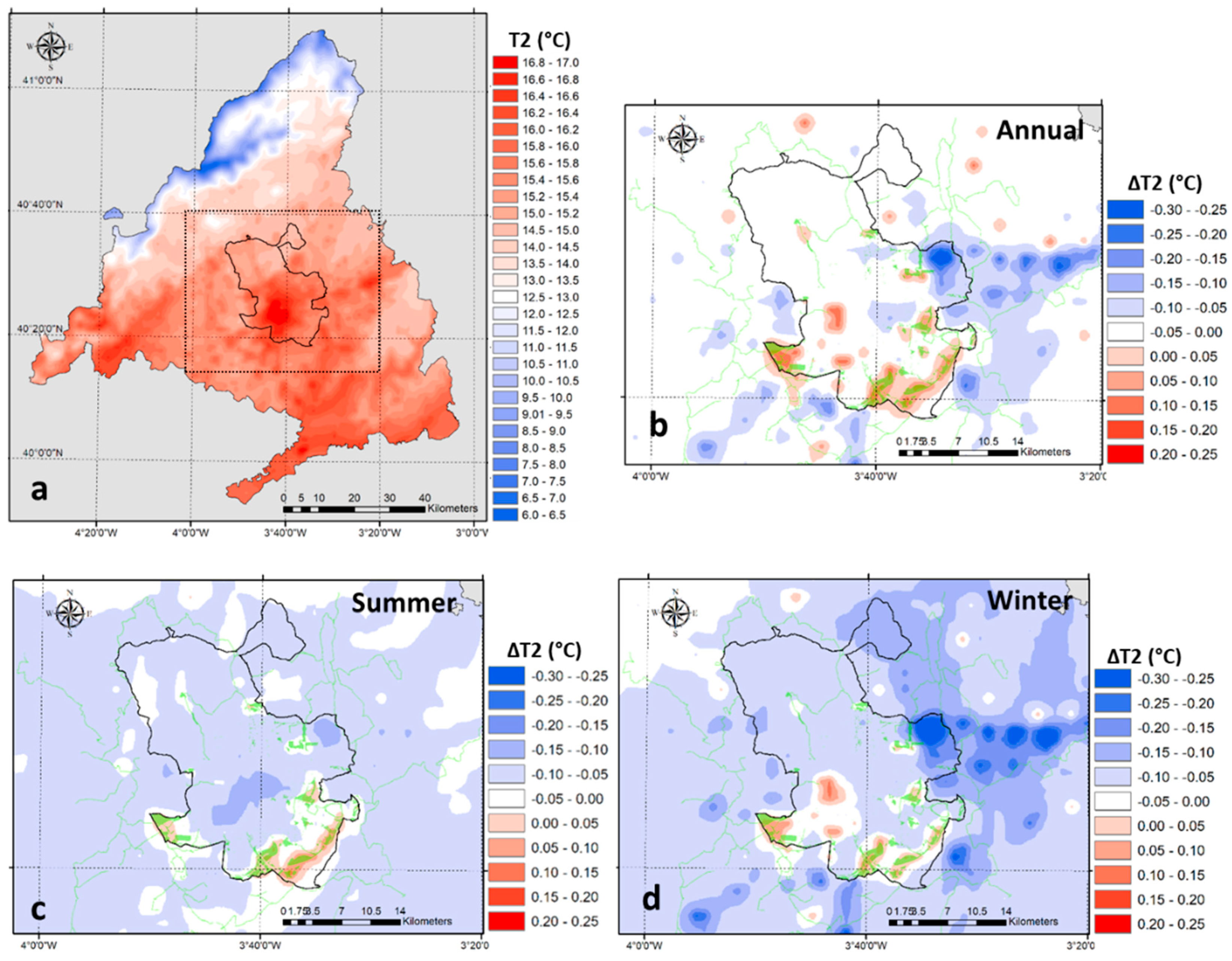
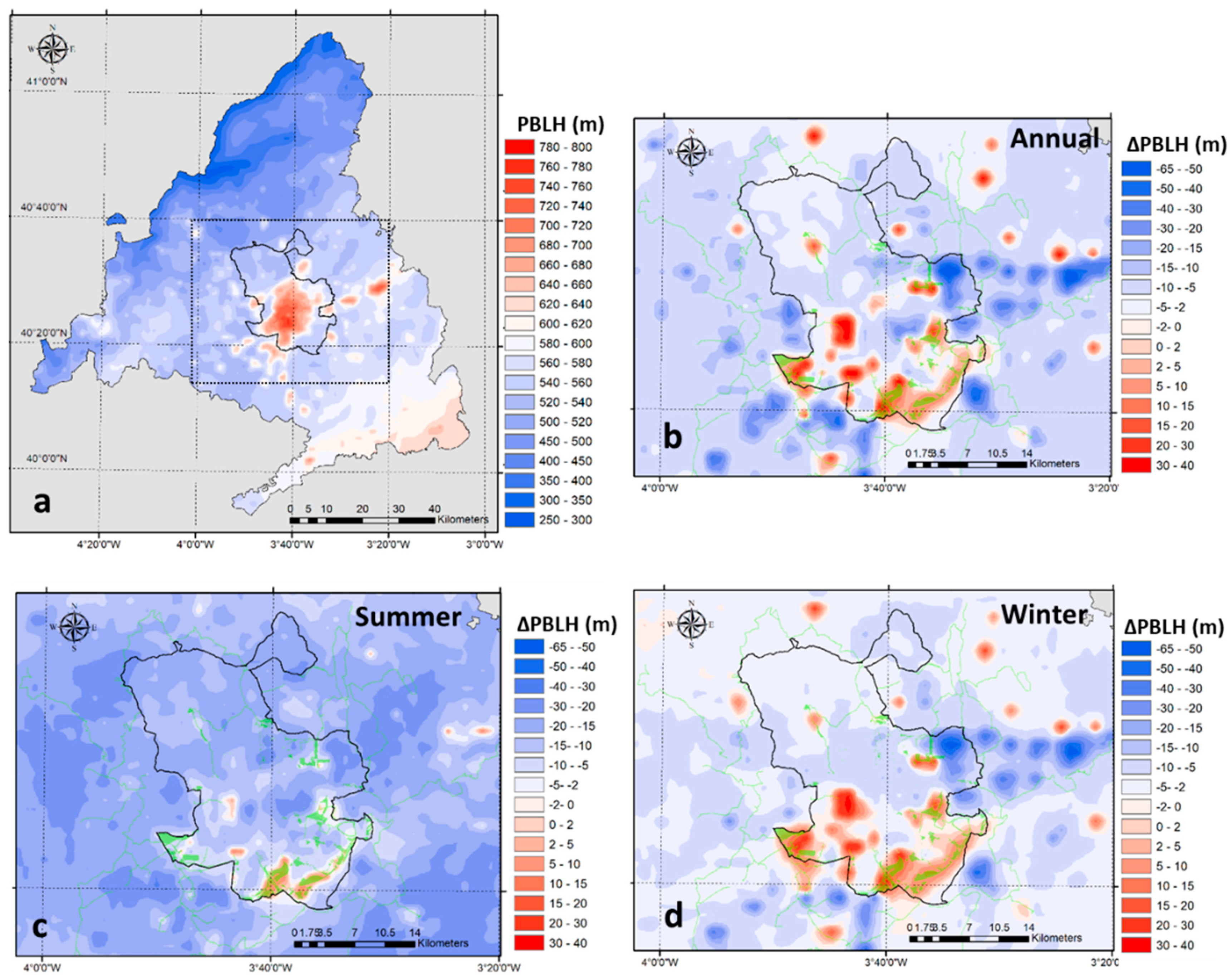
3.1. Impact of NBS on Meteorology

Figure 4a presents the annual mean temperature at ground level (T2) for the Baseline Scenario. This image clearly shows the heat-island effect of Madrid city in the center of the modeling domain. Topography also plays an important role, explaining the large temperature differences between the northern limit of the Madrid Region (6–10 °C) that corresponds to the ‘Sierra de Guadarrama’ mountain range (2000–2400 m height above sea level) and the southern part of the modeling domain, with annual mean temperatures up to 17 °C in the ‘Tajuña’ and ‘Henares’ valleys. Figure 4b–d show the difference between the Future Scenario and the Baseline Scenario for T2 as an annual mean as well as the summer and winter mean, respectively. Positive values (>0), represented in red, correspond to increments, while negative values (in blue) indicate a decrease induced by future NBS (represented in light green). In all three figures, we observe positive values in the close vicinity of interventions. Of note, the introduction of trees in barren areas brings about air temperature increases up to 0.20 °C (Table 2) (1%, Figure S1). This increase may be related to augmented sensible-heat (SH) flux in the areas where new trees are included (Figure S2), due to a decrease in albedo and enhanced energy absorption (Figure S3). Overall SH fluxes are considerably higher than latent heat (LH), something typical of relatively dry soils [67,68].
Although T2 increases over more extended areas during winter (Figure 4), increased evapotranspiration in summer strengthens the heat transfer from the atmosphere to the surface and may offset upward fluxes, causing a net cooling effect [69].
On the other hand, increasing the vegetation within the city (e.g., the area affected by ‘Madrid Nuevo Norte’) produces reductions in annual average temperature of up to 0.15 °C, due to lower energy absorption rates (higher albedo and lower heat capacity) along with increased evapotranspiration.
In addition to local changes, we observe temperature variations in areas not directly affected by the introduction of vegetation, such as the Henares and Jarama valley (northeast of our modelling domain, Figure S4). The cooling effect in that area is presumably related to changes in wind patterns, both in speed (Figure 5b) and direction (Figure S5), that lead to cooler air advection and alter surface heat balance.
Annual average changes in wind speed (at a 10 m height) are shown in Figure 5a. The model outputs from the baseline simulations clearly show that wind speed within Madrid City is 2–3 m s−1 lower than that of nearby rural areas. In contrast, the highest average values are found in the mountain range up north, with annual average values up to 7.5 m s−1. The impact of the envisaged NBS on those average values is presented in Figure 5b. Our model results suggest that new vegetation may considerably reduce wind speed (blue tones), of up to 0.4 m s−1 (Table 2) in the locations where more substantial interventions are planned, such as in the southeastern area of the modelling domain. As shown in Figure S1, in relative terms, annual average wind speed shows 5%–10% reductions in most of the urban area. This seems to be related to dramatic changes in the roughness length (e.g., Figure 3) in previously unwooded natural areas (Figure 2). As a consequence, we observe friction velocity (a turbulence scale) increases of up to 0.2 m s−1. Although mainly evergreen species are considered in the reforestation of ‘Bosque Metropolitano’ (Quercus ilex, Pinnus Pinea and Pinus halepensis predominantly), this effect is stronger in summer (Figure S5), when maximum LAI values are reached [70]. The results shown in Figure 4 suggest that the effect on a given location may depend on mesoscale phenomena, since wind speed changes can be seen in areas not directly affected by NBS. Increased friction and reduced advection may cause wind speed increases in the surroundings of interventions, an effect that may be modulated by regional circulation associated to topographical features. In this particular case, we observe increases in wind speed of up to 0.3 m s−1 in winter in the Henares and Jarama Valleys (Figure S4).
Our Future-Scenario simulation also indicates that new vegetation may induce changes in wind directions, more evidently during summer (Figure S5), of up to 10° as an average in summer. Wind shifts concentrate on the Jarama and Henares valleys (east and northeast of our modelling domain), suggesting that local topography is an important factor for the impact of NBS on meteorology.
Finally, we show the impact of planned NBS on the PBLH, identified as a critical variable for ambient concentration levels in this particular area in previous studies [66]. This meteorological variable is closely related to the amount of turbulence, both thermal and mechanical, generated by the surface. Consequently, it is clear in Figure 6a that, currently, average PBLH is considerably higher in built-up areas, with mean values in downtown Madrid of up to 800 m (around 600 m in winter and 1000 m in summer). The changes from the baseline scenario are also dependent on changes in vertical heat fluxes and mechanical turbulence. We observe that PBLH changes are dominated by convective processes and, thus, it matches the changes described for T2. Consequently, we observe a generalized drop, of up to 65 m of PBLH in summer (Figure 6c), and increases in winter (of up to 40 m) in the close vicinity of the main interventions. While the variations are similar in absolute terms, they are relatively more important in winter (8% in comparison to a maximum value of 4% in summer, as shown in Figure S1).
Figure 6b shows contrasting results for the annual mean value and strong spatial gradients, from 250 m in the mountain range up to 800 m in downtown Madrid. This is consistent with previous studies that have reported PBLH variation in short spatial scales due to differential heating of different surfaces and land uses [71].

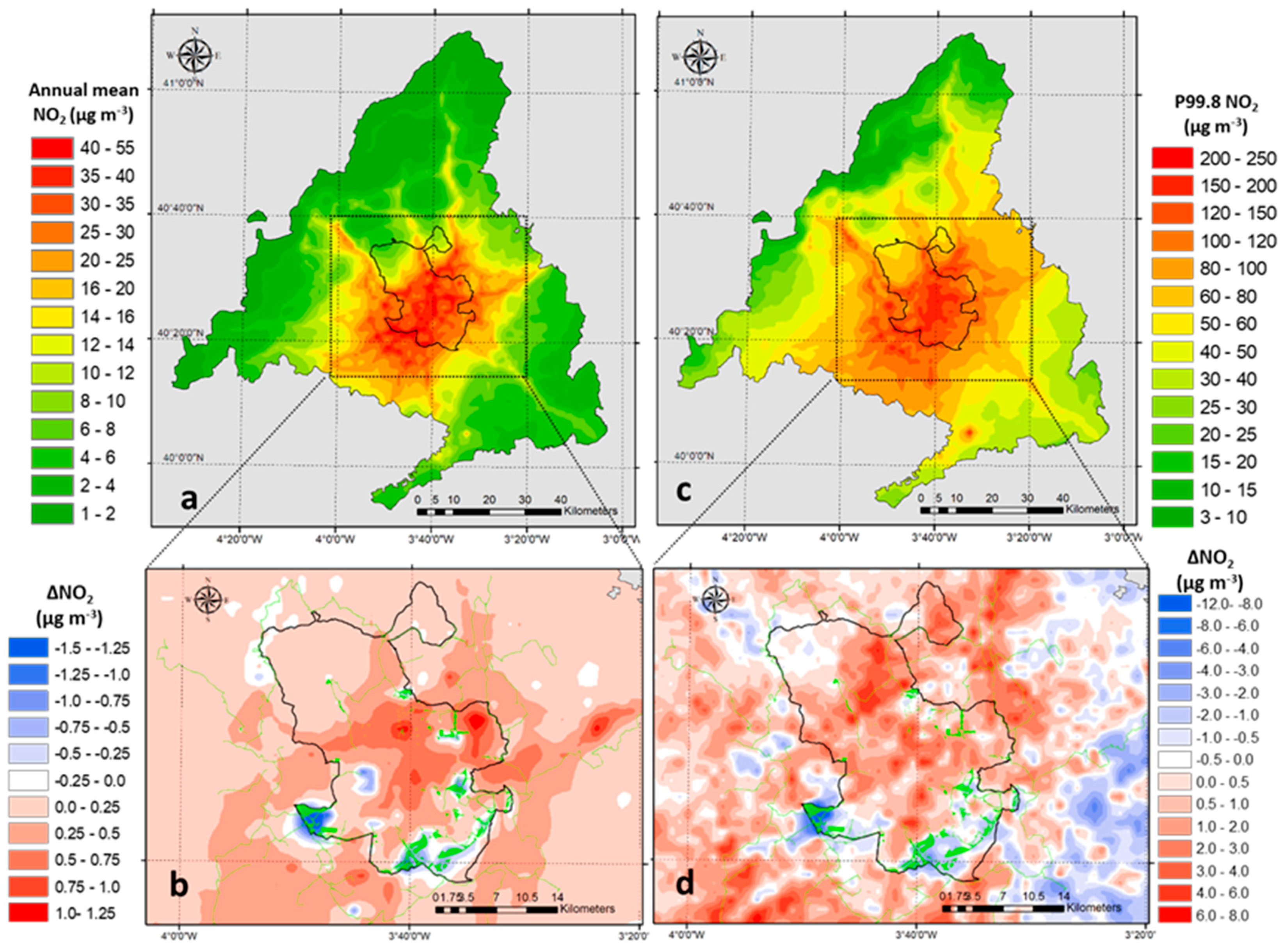
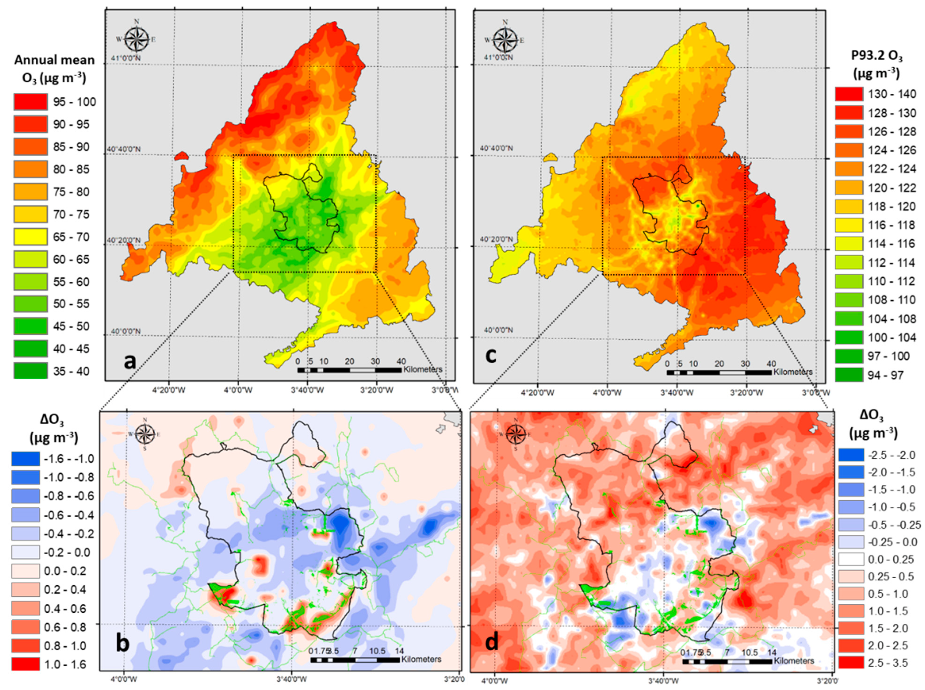
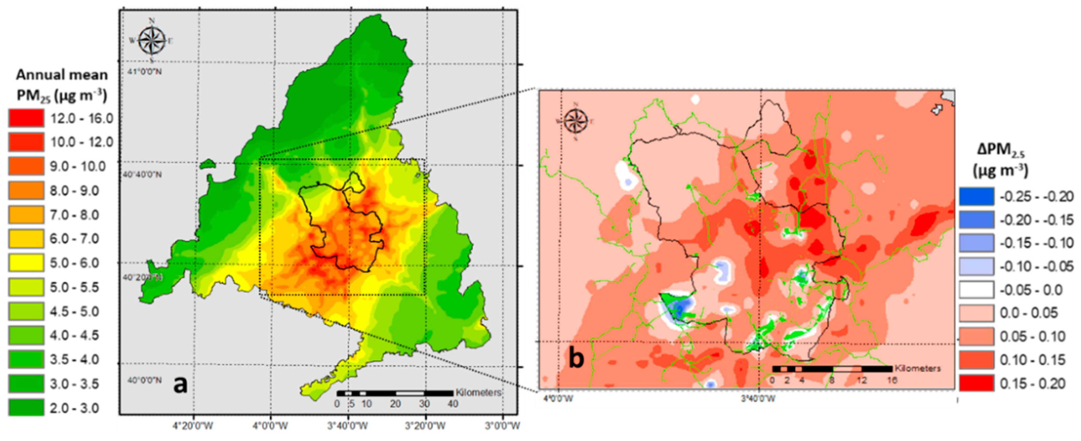
3.2. Impact of NBS on Air Quality

The assessment of the influence of future vegetation on air quality is based on the limit and target values defined by the Air Quality European Directive (2008/50/EC) for the protection of human health (Table S3).
Figure 7 shows the results for NO2. This is a very important pollutant in Madrid since it has been the main target of previous pollution-control measures in both long- [55] and short-term [66] actions plans. Figure 7a shows the annual mean concentration for the Baseline Scenario (current situation). The highest concentration levels are found in downtown Madrid and in the main radial highways, where road traffic emissions [72] cause exceedances of the annual limit value for the protection of human health (40 µg/m3). Figure 7b shows the expected changes in annual mean NO2 due to the implementation of NBS in Madrid. Similarly to the results discussed for meteorological variables, the main differences between the Future and Baseline scenarios occur around the intervention areas (blue values imply concentration reductions, i.e., air-quality improvements, while red tones indicate the opposite). We found local reductions in NO2 average concentrations of up to 1.5 µg m−3 (Table 3) (a 3–4% increase in relative terms, as illustrated in Figure S6) in those grid cells where temperature is increased (currently-treeless areas around the city). The increase in heat fluxes and, most importantly, turbulence intensity rise the mixing height, which contributes to reducing the concentration of this pollutant. Conversely, we found slight concentration increases (0.5%–0.75 µg m−3, 2%–3%) elsewhere in the city, especially downtown Madrid (‘Madrid Nuevo Norte’), where the future vegetation has a net cooling effect. It should be noted that additional sensitivity tests (not shown) confirm that concentration changes are mainly driven by the NBS impact on meteorological conditions and not so much for the increase of biogenic emissions. As expected, O3 levels vary in the opposite direction (Figure 8b), since decreases in NOX imply less titration of NO and, thus, less consumption of O3 to produce NO2 [73].
As for NO2 peak values, represented by the hourly percentile 99.8 (19th highest value within the calendar year), the spatial patterns are similar to those of the annual mean in the Baseline Scenario. In this case, we observe maximum values for the NO2 hourly limit value close to 250 µg m−3 (Figure 7c). Future vegetation (Figure 7d) would reduce these peaks in the range of 4–11 µg m−3 (2%–8% according to Figure S6) in the more densely reforested areas of ‘Bosque Metropolitano’. Increments of up to 5 µg m−3 occur in some urban locations, presumably due to a decreased PBLH associated to the vegetation cooling effect within the city. A thinner mixing height may promote the accumulation of pollutants and give rise to slightly higher concentration levels [71,74].
Regarding changes in O3 maximum daily eight-hour means (Figure 8d), slight increments of around 3 µg m−3 (below 1%) are predicted in those locations where NO2 peak values are expected to decline. Again, O3 may be reduced in the city center, due to NO2 increments. Contrarily to the effects found for the O3 annual mean (not regulated), O3 may marginally increase as well in non-urban areas, far from the envisaged NBS. This may be related to slower reactions involving VOCs [75]; although specific analyses would be needed to provide an accurate explanation.
The results for PM10, summarized in Figure 9, show that current concentration patterns (Figure 9a,c) are strongly influenced by the prevailing NE-SW wind direction that disperse emissions from the city in that direction. As for the changes induced by future vegetation on this pollutant, maximum reductions of 0.3 µg m−3and 1.0 µg m−3 (Table 3) (1%–2% and 2%–3%, respectively, as illustrated in Figure S7) are predicted for the annual mean (Figure 9b) and the 36th highest 24-h mean (Figure 9d), respectively. The model anticipates some concentration increases within the city, specifically in the area affected by ‘Madrid Nuevo Norte’. In this case, the substitution of urban fabric by natural cover leads to a cooling effect that contracts the PBL, causing slight increments of PM10 ambient concentration (of around 0.2 µg m−3, as an annual mean). It should be noted that both the NO2 and PM expected increments are very small in relative terms (around 3% and 1%, respectively). The relatively smaller increment of PM ambient concentration may be related to a higher deposition rate that affects particulate matter more intensely.
We found very similar results for finer particles (PM2.5). As illustrated in Figure 10, very limited concentration decreases (of slightly higher than 0.2 µg m−3 as an annual mean, approximately 2%) would occur in new wooden areas in the city outskirts. The combined effect of wind reduction and direction modification with reduced mixing height may result in generalized concentration increases in the metropolitan area of the city, if constant emissions are assumed.

4. Conclusions

In this study, we describe and apply a methodology to assess the impact of urban vegetation at a city scale through a modelling approach. In particular, we investigate how future vegetation plans in Madrid may affect meteorology and air quality. Our results reveal that NBS may have a significant impact on important meteorological features, such as temperature, wind fields and planetary boundary layer height. Depending on the location of new vegetation, we found contrasting results. Interventions in consolidated urban areas (‘Barrios productores’ and ‘Madrid Nuevo Norte’) are expected to have a predominant cooling effect, while the introduction of vegetation in barren or scarcely vegetated areas in the city outskirts (‘Arco Verde’ and, mainly, ‘Bosque Metropolitano’) would induce average temperature increases. NBS generally increase friction, acting as a momentum sink and, thus, enhancing vertical mixing but reducing wind speed. However, we found that the impact on mixing height is dominated by thermal effects. As a result, under a constant-emission scenario, ambient concentration levels of NO2 and PM would show moderate changes in the close vicinity of the interventions. Moderate changes are also predicted for O3 concentrations due to future interventions, opposite in kind to those of NO2. We also observe that NBS may have slight effects in relatively distant locations. In addition to the potential of vegetation to modify wind flows, this phenomenon strongly depends on local features (land uses and topography), so the impact of other interventions at a regional level cannot be anticipated.
Our findings suggest that vegetation may have significant effects locally, mainly due to its impact on urban meteorology, but it is essential to perform site-specific simulations from regional to local scales to take into account not only vegetation features but also other factors affecting regional atmospheric dynamics and chemical processes, such as land uses and topography. In addition, we conclude that vegetation may decrease pollutant concentration levels in some areas for some pollutants but also increase their concentration elsewhere. Therefore, it is necessary to combine NBS with further anthropogenic emission abatement measures. The proposed methodology could be used to assess the combined effect of NBS and emission-reduction measures within air-quality plans for urbanized areas.

Supplementary Materials

The following supporting information can be downloaded at: https://0-www-mdpi-com.brum.beds.ac.uk/article/10.3390/f13050690/s1, Table S1. Dimensions and spatial resolution of WRF and CMAQ modelling domains; Table S2. Air quality parameter regulated by the Directive 2008/50/EC on ambient air quality and cleaner air for Europe; Table S3. Properties of relevant natural-land uses (WRF VEGPARM file); Table S4. Statistics: NOAA meteorological stations; Table S5. Statistics: Madrid meteorological stations; Figure S1. Annual mean temperature, wind speed (10 m) and PBL height relative changes (100 × (Future − Baseline) / Baseline); Figure S2. Seasonal mean variation (Future − Baseline) sensible heat flux (W m−2) at the surface in summer (a) and winter (b). Seasonal mean variation (Future − Baseline) latent heat flux at the surface in summer (c) and winter (d); Figure S3. Seasonal mean variation (Future − Baseline) of solar radiation absorbed at ground in winter (a) and summer (b); Figure S4. Detailed topographic map of the study area; Figure S5. Seasonal mean variation (Future − Baseline) of friction velocity (∆USTAR) and wind speed in summer (a) and winter (b). Seasonal mean variation (Future − Baseline) wind direction in summer (c) and winter (d); Figure S6. NO2 and O3 relative changes (100 × (Future − Baseline) / Baseline); Figure S7. PM10 and PM2.5 relative changes (100 × (Future − Baseline) / Baseline).

Author Contributions

Conceptualization: D.d.l.P., J.M.d.A., A.N., C.S., S.F. (Sandro Finardi), S.F. (Silvano Fares), L.T., R.B. and M.M.; Methodology: D.d.l.P., J.M.d.A., R.B. and M.M.; Software: D.d.l.P. and C.S.; Validation: A.N., S.F. (Sandro Finardi) and S.F. (Silvano Fares); Formal analysis: D.d.l.P., J.M.d.A. and R.B.; Investigation: D.d.l.P., J.M.d.A., A.N., C.S., S.F. (Sandro Finardi), S.F. (Silvano Fares), L.T., R.B. and M.M.; Resources: D.d.l.P., C.S. and S.F. (Sandro Finardi); Data Curation: D.d.l.P., J.M.d.A., L.T., R.B. and M.M.; Writing—original draft preparation: D.d.l.P., J.M.d.A. and R.B.; Writing—review and editing: D.d.l.P., J.M.d.A., A.N., C.S., S.F. (Sandro Finardi), S.F. (Silvano Fares), L.T., R.B. and M.M.; Visualization: D.d.l.P.; Supervision: R.B.; Project Administration: M.M.; Funding Acquisition: S.F. (Sandro Finardi), S.F. (Silvano Fares), L.T., R.B. and M.M. All authors have read and agreed to the published version of the manuscript.

Funding

This study was developed under the project Life VEG-GAP (https://www.lifeveggap.eu/) Accessed 20 April 2022) which was funded by European Union Life Program in 2018, Grant Number LIFE18 PRE IT 003.

Data Availability Statement

Data available in Information platform: https://veggaplatform.enea.it (accessed on 27 April 2022).

Acknowledgments

We acknowledge Madrid’s Air Quality Service for providing meteorological dataset from the City Hall meteorological network.

Conflicts of Interest

The authors declare no conflict of interest.

References

  1. EEA. Climate Change, Impacts and Vulnerability in Europe 2016—An Indicator-Based Report; EEA Report No 1/2017; Publications Office of the European Union: Luxembourg; European Environment Agency: Copenhagen, Denmark, 2017; ISBN 978-92-9213-835-6. [Google Scholar] [CrossRef]
  2. IPCC. Global Warming of 1.5 °C; Intergovernmental Panel on Climate Change: Geneva, Switzerland, 2018; Available online: http://www.ipcc.ch/report/sr15/ (accessed on 2 January 2022).
  3. IPCC. Climate Change and Land—An IPCC Special Report on Climate Change, Desertification, Land Degradation, Sustainable Land Management, Food Security, and Greenhouse Gas Fluxes in Terrestrial Ecosystems; Summary for policymakers, Intergovernmental Panel on Climate Change: Geneva, Switzerland, 2019; Available online: https://www.ipcc.ch/site/assets/uploads/sites/4/2020/02/SPM_Updated-Jan20.pdf (accessed on 24 February 2022).
  4. EEA. Nature-Based Solutions in Europe: Policy, Knowledge and Practice for Climate Change Adaptation and Disaster Risk Reduction; EEA Report No 01/2021; Publications Office of the European Union: Luxembourg; European Environment Agency: Copenhagen, Denmark, 2021; ISBN 978-92-9480-362-7. [Google Scholar] [CrossRef]
  5. Kim, G.; Coseo, P. Urban Park Systems to Support Sustainability: The Role of Urban Park Systems in Hot Arid Urban Climates. Forests 2018, 9, 439. [Google Scholar] [CrossRef] [Green Version]
  6. Hanson, H.I.; Wickenberg, B.; Olsson, J.A. Working on the boundaries—How do science use and interpret the nature-based solution concept? Land Use Policy 2020, 90, 104302. [Google Scholar] [CrossRef]
  7. Wickenberg, B.; McCormick, K.; Olsson, J.A. Advancing the implementation of nature-based solutions in cities: A review of frameworks. Environ. Sci. Policy 2021, 125, 44–53. [Google Scholar] [CrossRef]
  8. WHO. World Health Statistics 2016: Monitoring Health for the SDGs Sustainable Development Goals; World Health Organization: Geneva, Switzerland, 2016; ISBN 978 92 4 156526 4. [Google Scholar]
  9. OPPLA. European Union Repository of Nature-Based Solutions. 2022. Available online: https://oppla.eu/case-study-finder (accessed on 10 January 2022).
  10. Lafortezza, R.; Chen, J.; van den Bosch, C.K.; Randrup, T.B. Nature-based solutions for resilient landscapes and cities. Environ. Res. 2018, 165, 431–441. [Google Scholar] [CrossRef]
  11. Zwierzchowska, I.; Fagiewicz, K.; Poniży, L.; Lupa, P.; Mizgajski, A. Introducing nature-based solutions into urban policy—facts and gaps. Case study of Poznań. Land Use Policy 2019, 85, 161–175. [Google Scholar] [CrossRef]
  12. Rendón, O.R.; Sandorf, E.D.; Beaumonta, N.J. Heterogeneity of values for coastal flood risk management with nature-based solutions. J. Environ. Manag. 2022, 304, 114212. [Google Scholar] [CrossRef]
  13. Hynes, S.; Burger, R.; Tudella, J.; Norton, D.; Chen, W. Estimating the costs and benefits of protecting a coastal amenity from climate change-related hazards: Nature based solutions via oyster reef restoration versus grey infrastructure. Ecol. Econ. 2022, 194, 107349. [Google Scholar] [CrossRef]
  14. Lallemant, D.; Hamel, P.; Balbi, M.; Lim, T.N.; Schmitt, R.; Win, S. Nature-based solutions for flood risk reduction: A probabilistic modeling framework. One Earth 2021, 4, 1310–1321. [Google Scholar] [CrossRef]
  15. Langergraber, G.; Masi, F. Treatment wetlands in decentralised approaches for linking sanitation to energy and food security. Water Sci. Technol. 2018, 77, 859–860. [Google Scholar] [CrossRef]
  16. Coventry, P.A.; Brown, J.V.E.; Pervin, J.; Brabyn, S.; Pateman, R.; Breedvelt, J.; Gilbody, S.; Stancliffe, R.; McEachan, R.; White, P.C.L. Nature-based outdoor activities for mental and physical health: Systematic review and meta-analysis. SSM Popul. Health 2021, 16, 100934. [Google Scholar] [CrossRef]
  17. Keskinen, K.E.; Rantakokko, M.; Suomi, K.; Rantanen, T.; Portegijs, E. Nature as a facilitator for physical activity: Defining relationships between the objective and perceived environment and physical activity among community-dwelling older people. Health Place 2018, 49, 111–119. [Google Scholar] [CrossRef] [PubMed]
  18. Croeser, T.; Garrard, G.; Roshan, S.; Ossola, A.; Bekessy, S. Choosing the right nature-based solutions to meet diverse urban challenges. Urban For. Urban Green. 2021, 65, 127337. [Google Scholar] [CrossRef]
  19. Carvalho, P.N.; Finger, D.C.; Masi, F.; Cipolletta, G.; Oral, H.V.; Tóth, A.; Regelsberger, M.; Exposito, A. Nature-based solutions addressing the water-energy-food nexus: Review of theoretical concepts and urban case studies. J. Clean Prod. 2022, 338, 130652. [Google Scholar] [CrossRef]
  20. Ignatieva, M.; Eriksson, F.; Eriksson, T.; Berg, P.; Hedblom, M. The lawn as a social and cultural phenomenon in Sweden. Urban For. Urban Green. 2017, 21, 213–223. [Google Scholar] [CrossRef]
  21. Sung, C.Y. Mitigating surface urban heat island by a tree protection policy: A case study of The Woodland, Texas, USA. Urban For. Urban Green. 2013, 12, 474–480. [Google Scholar] [CrossRef]
  22. Grote, R.; Samson, R.; Alonso, R.; Amorim, J.H.; Cariñanos, P.; Churkina, G.; Fares, S.; Thiec, D.L.; Niinemets, Ü.; Mikkelsen, T.N. Functional traits of urban trees: Air pollution mitigation potential. Front. Ecol. Environ. 2016, 14, 543–550. [Google Scholar] [CrossRef]
  23. Gong, C.; Xian, C.; Ouyang, Z. Assessment of NO2 Purification by Urban Forests Based on the i-Tree Eco Model: Case Study in Beijing, China. Forests 2022, 13, 369. [Google Scholar] [CrossRef]
  24. Zafra-Mejía, C.; Suárez-López, J.; Rondón-Quintana, H. Analysis of Particulate Matter Concentration Intercepted by Trees of a Latin-American Megacity. Forests 2021, 12, 723. [Google Scholar] [CrossRef]
  25. Bonn, B.; von Schneidemesser, E.; Butler, T.; Churkina, G.; Ehlers, C.H.; Grotea, R.; Klemp, D.; Nothard, R.; Schäfe, K.; von Stülpnagel, A.; et al. Impact of vegetative emissions on urban ozone and biogenic secondary organic aerosol: Box model study for Berlin, Germany. J. Clean Prod. 2018, 176, 827–841. [Google Scholar] [CrossRef]
  26. Kasprzyk, I.; Ćwik, A.; Kluska, K.; Wójcik, T.; Cariñanos, P. Allergenic pollen concentrations in the air of urban parks in relation to their vegetation. Urban For. Urban Green. 2019, 46, 126486. [Google Scholar] [CrossRef]
  27. Lara, B.; Rojo, J.; Fernández-González, F.; González-García-Saavedra, A.; Serrano-Bravo, M.D.; Pérez-Badia, R. Impact of Plane Tree Abundance on Temporal andSpatial Variations in Pollen Concentration. Forests 2020, 11, 817. [Google Scholar] [CrossRef]
  28. Speak, A.; Escobedo, F.J.; Russo, A.; Zerbea, S. An ecosystem service-disservice ratio: Using composite indicators to assess the net benefits of urban trees. Ecol. Indic. 2018, 95, 544–553. [Google Scholar] [CrossRef]
  29. Guenther, A.; Hewitt, C.N.; Erickson, D.; Fall, R.; Geron, C.; Graedel, T.; Harley, P.; Klinger, L.; Lerdau, M.; Mckay, W.A.; et al. A global model of natural volatile organic compound emissions. J. Geophys. Res. 1995, 100, 8873–8892. [Google Scholar] [CrossRef]
  30. Sindelarova, K.; Granier, C.; Bouarar, I.; Guenther, A.; Tilmes, S.; Stavrakou, T.; Müller, J.-F.; Kuhn, U.; Stefani, P.; Knorr, W. Global data set of biogenic VOC emissions calculated by the MEGAN model over the last 30 years. Atmos. Chem. Phys. Eur. Geosci. Union 2014, 14, 9317–9341. [Google Scholar] [CrossRef] [Green Version]
  31. Sartelet, K.N.; Couvidat, F.; Seigneur, C.; Roustan, Y. Impact of biogenic emissions on air quality over Europe and North America. Atmos. Environ. 2012, 53, 131–141. [Google Scholar] [CrossRef] [Green Version]
  32. Tagaris, E.; Sotiropoulou, R.E.P.; Gounaris, N.; Andronopoulos, S.; Vlachogiannis, D. Impact of biogenic emissions on ozone and fine particles over Europe: Comparing effects of temperature increase and a potential anthropogenic NOx emissions abatement strategy. Atmos. Environ. 2014, 98, 214–223. [Google Scholar] [CrossRef]
  33. Gao, Y.; Ma, M.; Yan, F.; Su, H.; Wang, S.; Liao, H.; Zhao, B.; Wang, X.; Sun, Y.; Hopkins, J.R.; et al. Impacts of biogenic emissions from urban landscapes on summer ozone and secondary organic aerosol formation in megacities. Sci. Total Environ. 2022, 814, 152654. [Google Scholar] [CrossRef]
  34. Marchetti, P.; Pesce, G.; Villani, S.; Antonicelli, L.; Ariano, R.; Attena, F.; Bono, R.; Bellisario, V.; Fois, A.; Gibelli, N.; et al. Pollen concentra-tions and prevalence of asthma and allergic rhinitis in Italy: Evidence from the GEIRD study. Sci. Total Environ. 2017, 584–585, 1093–1099. [Google Scholar] [CrossRef]
  35. Idrose, N.S.; Dharmage, S.C.; Lowe, A.J.; Lambert, K.A.; Lodge, C.J.; Abramson, M.J.; Douglass, J.A.; Newbigin, E.J.; Erbas, B. A systematic review of the role of grass pollen and fungi in thunderstorm asthma. Environ. Res. 2020, 181, 108911. [Google Scholar] [CrossRef]
  36. Davis, A.Y.; Jung, J.; Pijanowski, B.C.; Minor, E.S. Combined vegetation volume and “greenness” affect urban air temperature. Appl. Geogr. 2016, 71, 106–114. [Google Scholar] [CrossRef] [Green Version]
  37. Crum, S.M.; Shiflett, S.A.; Jenerette, G.D. The influence of vegetation, mesoclimate and meteorology on urban atmospheric microclimates across a coastal to desert climate gradient. J. Environ. Manag. 2017, 200, 295–303. [Google Scholar] [CrossRef]
  38. Rui, L.; Buccolieri, R.; Gao, Z.; Ding, W.; Shen, J. The Impact of Green Space Layouts on Microclimate and Air Quality in Residential Districts of Nanjing, China. Forests 2018, 9, 224. [Google Scholar] [CrossRef] [Green Version]
  39. Cowie, S.M.; Knippertz, P.; Marsham, J.H. Are vegetation-related roughness changes the cause of the recent decrease in dust emission from the Sahel? Geophys. Res. Lett. 2013, 40, 1868–1872. [Google Scholar] [CrossRef] [PubMed] [Green Version]
  40. Meng, Z.; Dang, X.; Gao, Y.; Ren, X.; Ding, Y.; Wang, M. Interactive effects of wind speed, vegetation coverage and soil moisture in controlling wind erosion in a temperate desert steppe, Inner Mongolia of China. J. Arid Land 2018, 10, 534–547. [Google Scholar] [CrossRef] [Green Version]
  41. Bo, L.; Chen, L.; Qingshan, Y.; Yuji, T.; Xinxin, Z. Full-scale wind speed spectra of 5 Year time series in urban boundary layer observed on a 325 m meteorological tower. J. Wind. Eng. Ind. Aerodyn. 2021, 218, 104791. [Google Scholar] [CrossRef]
  42. Wang, M.; Tang, G.; Liu, Y.; Ma, M.; Yu, M.; Hu, B.; Zhang, Y.; Wang, Y.; Wang, Y. The difference in the boundary layer height between urban and suburban areas in Beijing and its implications for air pollution. Atmos. Environ. 2021, 260, 118552. [Google Scholar] [CrossRef]
  43. Huang, Y.; Guo, B.; Sun, H.; Liu, H.; Chen, S.X. Relative importance of meteorological variables on air quality and role of boundary layer height. Atmos. Environ. 2021, 267, 118737. [Google Scholar] [CrossRef]
  44. Gómez-Moreno, F.J.; Artíñano, B.; Díaz Ramiro, E.; Barreiro, M.; Núñez, L.; Coz, E.; Dimitroulopoulou, C.; Vardoulakis, S.; Yagüe, C.; Maqueda, G.; et al. Urban vegetation and particle air pollution: Experimental campaigns in a traffic hotspot. Environ. Pollut. 2019, 247, 195–205. [Google Scholar] [CrossRef]
  45. Santiago, J.L.; Buccolieri, R.; Rivas, E.; Calvete-Sogo, H.; Sanchez, B.; Martilli, A.; Alonso, R.; Elustondo, D.; Santamaría, J.S.; Martín, F. CFD modelling of vegetation barrier effects on the reduction of traffic related pollutant concentration in an avenue of Pamplona, Spain. Sustain. Cities Soc. 2019, 48, 101559. [Google Scholar] [CrossRef]
  46. Santiago, J.L.; Buccolieri, R.; Rivas, E.; Sanchez, B.; Martilli, A.; Gatto, E.; Martín, F. On the Impact of Trees on Ventilation in a Real Street in Pamplona, Spain. Atmosphere 2019, 10, 697. [Google Scholar] [CrossRef] [Green Version]
  47. Jeong, N.-R.; Han, S.-W.; Kim, J.-H. Evaluation of Vegetation Configuration Models for Managing Particulate Matter along the Urban Street Environment. Forests 2022, 13, 46. [Google Scholar] [CrossRef]
  48. Pearce, H.; Levine, J.G.; Cai, X.; MacKenzie, A.R. Introducing the Green Infrastructure for Roadside Air Quality (GI4RAQ) Platform: Estimating Site-Specific Changes in the Dispersion of Vehicular Pollution Close to Source. Forests 2021, 12, 769. [Google Scholar] [CrossRef]
  49. Alonso, A.; Vivanco, M.G.; González-Fernández, I.; Bermejo, V.; Palomino, I.; Garrido, J.L.; Elvira, S.; Salvador, P.; Artíñano, B. Modelling the influence of peri-urban trees in the air quality of Madrid region (Spain). Environ. Pollut. 2011, 159, 2138–2147. [Google Scholar] [CrossRef] [PubMed]
  50. Skamarock, W.C.; Klemp, J.B. A time-split nonhydrostatic atmospheric model for weather research and forecasting applications. J. Comput. Phys. 2008, 227, 3465–3485. [Google Scholar] [CrossRef]
  51. Martilli, A.; Clappier, A.; Rotach, M.W. An urban surface exchange parameterisation for mesoscale models. Bound. Layer Meteor. 2002, 104, 261–304. [Google Scholar] [CrossRef]
  52. Borge, R.; Alexandrov, V.; Del Vas, J.J.; Lumbreras, J.; Rodríguez, E. A comprehensive sensitivity analysis of the WRF model for air quality applications over the Iberian Peninsula. Atmos. Environ. 2008, 42, 8560–8574. [Google Scholar] [CrossRef]
  53. de la Paz, D.; Borge, R.; Martilli, A. Assessment of a high resolution annual WRF-BEP/CMAQ simulation for the urban area of Madrid (Spain). Atmos. Environ. 2016, 144, 282–296. [Google Scholar] [CrossRef]
  54. Baek, B.H.; Seppanen, C. Sparse Matrix Operator Kernel Emissions (SMOKE) Modeling System (Version SMOKE User’s Documentation). Zenodo 2018. [Google Scholar] [CrossRef]
  55. Borge, R.; Lumbreras, J.; Pérez, J.; de la Paz, D.; Vedrenne, M.; de Andrés, J.M.; Rodríguez, M.E. Emission inventories and modeling requirements for the development of air quality plans. Application to Madrid (Spain). Sci. Total Environ. 2014, 466, 809–819. [Google Scholar] [CrossRef] [Green Version]
  56. Borge, R.; Lumbreras, J.; Rodríguez, E. Development of a high-resolution emission inventory for Spain using the SMOKE modelling system: A case study for the years 2000 and 2010. Environ. Modell. Softw. 2008, 23, 1026–1044. [Google Scholar] [CrossRef]
  57. Silibello, C.; Baraldi, R.; Rapparini, F.; Facini, O.; Neri, L.; Brilli, F.; Fares, S.; Finardi, S.; Magliulo, E.; Ciccioli, P.; et al. Modelling of biogenic volatile organic compounds emissions over Italy. In Proceedings of the 18th International Conference on Harmonisation within Atmospheric Dispersion Modelling for Regulatory Purposes (HARMO), Bologna, Italy, 9–12 October 2017. [Google Scholar]
  58. Byun, D.; Schere, K.L. Review of the Governing Equations, Computational Algorithms, and Other Components of the Models-3 Community Multiscale Air Quality (CMAQ) Modeling System. Appl. Mech. Rev. 2006, 59, 51–77. [Google Scholar] [CrossRef]
  59. Ching, J.; Byun, D. Introduction to the Models-3 framework and the Community Multiscale Air Quality model (CMAQ). In Science Algorithms of the EPA Models-3 Community Multiscale Air Quality (CMAQ) Modeling System; 20460. EPA/600/R-99/030; Office of Research and Development: Washington, DC, USA, 1999. [Google Scholar]
  60. Borge, R.; López, J.; Lumbreras, J.; Narros, A.; Rodríguez, E. Influence of boundary conditions on CMAQ simulations over the Iberian Peninsula. Atmos. Environ. 2010, 44, 2681–2695. [Google Scholar] [CrossRef]
  61. Yarwood, G.; Jung, J.; Whitten, G.; Heo, G.J.M.; Estes, M. Updates to the Carbon Bond Mechanism for Version 6 (CB6). In Proceedings of the 9th Annual CMAS Conference, Chapel Hill, NC, USA, 11–13 October 2010; pp. 1–4. [Google Scholar]
  62. Appel, K.W.; Pouliot, G.A.; Simon, H.; Sarwar, G.; Pye, H.O.T.; Napelenok, S.L.; Akhtar, F.; Roselle, S.J. Evaluation of dust and trace metal estimates from the Community Multiscale Air Quality (CMAQ) model version 5.0. Geosci. Model Dev. 2013, 6, 883–899. [Google Scholar] [CrossRef] [Green Version]
  63. Izquierdo, R.; Dos Santos, S.G.; Borge, R.; de la Paz, D.; Sarigiannis, D.; Gotti, A.; Boldo, E. Health impact assessment by the implementation of Madrid City air-quality plan in 2020. Environ. Res. 2020, 183, 109021. [Google Scholar] [CrossRef]
  64. Liu, Y.; Chen, F.; Warner, T.; Basara, J. Verification of a mesoscale data-assimilation and forecasting system for the Oklahoma City area during the Joint Urban 2003 field project. J. Appl. Meteorol. Climatol. 2006, 45, 912–929. [Google Scholar] [CrossRef]
  65. Borge, R.; Requia, W.J.; Yagüe, C.; Jhun, I.; Koutrakis, P. Impact of weather changes on air quality and related mortality in Spain over a 25-year period [1993–2017]. Environ. Int. 2019, 133, 105272. [Google Scholar] [CrossRef]
  66. Borge, R.; Artíñano, B.; Yagüe, C.; Gomez-Moreno, F.J.; Saiz-Lopez, A.; Sastre, M.; Narros, A.; García-Nieto, D.; Benavent, N.; Maqueda, G.; et al. Application of a short term air quality action plan in Madrid (Spain) under a high-pollution episode-Part I: Diagnostic and analysis from observations. Sci. Total Environ. 2018, 635, 1561–1573. [Google Scholar] [CrossRef]
  67. Castelli, F.; Entekhabi, D.; Caporali, E. Estimation of surface heat flux and an index of soil moisture using adjoint-state surface energy balance. Water Resour. Res. 1999, 35, 3115–3125. [Google Scholar] [CrossRef] [Green Version]
  68. Chen, F. The Noah land surface model in WRF: A short tutorial. LSM Group Meeting. 17 April 2007. Available online: https://www.atmos.illinois.edu/~snesbitt/ATMS597R/notes/noahLSM-tutorial.pdf (accessed on 10 January 2022).
  69. Li, Y.; Zhao, M.; Motesharrei, S.; Mu, Q.; Kalnay, E.; Li, S. Local cooling and warming effects of forests based on satellite observations. Nat. Commun. 2015, 6, 6603. [Google Scholar] [CrossRef] [Green Version]
  70. Yan, K.; Park, T.; Yan, G.; Liu, Z.; Yang, B.; Chen, C.; Nemani, R.R.; Knyazikhin, Y.; Myneni, R.B. Evaluation of MODIS LAI/FPAR product collection 6. Part 2: Validation and intercomparison. Remote Sens. 2016, 8, 460. [Google Scholar] [CrossRef] [Green Version]
  71. Hegarty, J.D.; Lewis, J.; McGrath-Spangler, E.L.; Henderson, J.; Scarino, A.J.; DeCola, P.; Ferrare, R.; Hicks, M.; Adams-Selin, R.D.; Welton, E.J. Analysis of the planetary boundary layer height during DISCOVER-AQ Baltimore–Washington, DC, with lidar and high-resolution WRF modeling. J. Appl. Meteorol. Climatol. 2018, 57, 2679–2696. [Google Scholar] [CrossRef]
  72. Borge, R.; Santiago, J.L.; de la Paz, D.; Martín, F.; Domingo, J.; Valdés, C.; Sanchez, B.; Rivas, E.; Rozas, M.T.; Lázaro, S.; et al. Application of a short term air quality action plan in Madrid (Spain) under a high-pollution episode-part II: Assess-ment from multi-scale modelling. Sci. Total Environ. 2018, 635, 1574–1584. [Google Scholar] [CrossRef] [PubMed]
  73. Saiz-Lopez, A.; Borge, R.; Notario, A.; Adame, J.A.; de la Paz, D.; Querol, X.; Artíñano, B.; Gómez-Moreno, F.J.; Cuevas, C.A. Unexpected increase in the oxidation capac-ity of the urban atmosphere of Madrid, Spain. Sci. Rep. 2017, 7, 45956. [Google Scholar] [CrossRef]
  74. Qu, Y.; Han, Y.; Wu, Y.; Gao, P.; Wang, T. Study of PBLH and its correlation with particulate matter from one-year observation over Nanjing, Southeast China. Remote Sens. 2017, 9, 668. [Google Scholar] [CrossRef] [Green Version]
  75. Jung, D.; de la Paz, D.; Notario, A.; Borge, R. Analysis of emissions-driven changes in the oxidation capacity of the atmosphere in Europe. Sci. Total Environ. 2022, 827, 154126. [Google Scholar] [CrossRef] [PubMed]
Figure 1. Nested modelling domains and detail of the innermost 1 km2 resolution domain showing dominant land-use types.
Forests 13 00690 g001
Figure 2. Baseline scenario along with the NBS-based interventions envisaged in the Future Scenario (left). Model grid cells affected by those vegetation changes and land-use category assigned in the Future Scenario (right).
Forests 13 00690 g002
Figure 3. Values of albedo, roughness length, emissivity and heat capacity for current (grey bars) and future (green bars) scenarios for a grid cell where new trees (‘Bosque Metropolitano’) are introduced.
Forests 13 00690 g003
Figure 4. Annual mean temperature for the Baseline Scenario (a). Expected variation in temperature: annual mean (b), summer mean (c) and winter mean (d), due to future vegetation.
Forests 13 00690 g004
Figure 5. Annual mean wind speed (10 m) for the Baseline Scenario (a). Expected variation in wind intensity: annual mean (b), summer mean (c) and winter mean (d), due to future vegetation.
Forests 13 00690 g005
Figure 6. Annual planetary boundary layer height (PBLH) for the Baseline Scenario (a). Expected variation of PBLH: annual mean (b), summer mean (c) and winter mean (d), due to future vegetation.
Forests 13 00690 g006
Figure 7. Annual mean of NO2 (µg m−3) for the Baseline Scenario (a) and expected variation (µg m−3) due to future vegetation (b). Hourly 99.8 NO2 percentile (µg m−3) for the Baseline Scenario (c) and expected variation (µg m−3) due to future vegetation (d).
Forests 13 00690 g007
Figure 8. Annual mean of O3 (µg m−3) for the Baseline Scenario (a) and expected variation (µg m−3) due to future vegetation (b). Daily percentile 93.2 of O3 maximum daily eight-hour mean (µg m−3) for the Baseline Scenario (c) and expected variation (µg m−3) due to future vegetation (d).
Forests 13 00690 g008
Figure 9. Annual mean of PM10 (µg m−3) for the Baseline Scenario (a) and expected variation (µg m−3) due to future vegetation (b). Daily 90.4 PM10 percentile (µg m−3) for the Baseline Scenario (c) and expected variation (µg m−3) due to future vegetation (d).
Forests 13 00690 g009
Figure 10. Annual mean of PM2.5 (µg m−3) for the Baseline Scenario (a) and expected variation (µg m−3) due to future vegetation (b).
Forests 13 00690 g010
Table 1. WRF model setup.
OptionSetup
InitializationERA5
Shortwave radiationMM5
Longwave radiationGFDL
Land-surface modelNoah LSM
Microphysics schemeWSM6
PBL schemeBoulac
Surface layer optionMonin–Obukhov
Cumulus parametrizationNo
Urban physicsBEP (building energy parameterization)
NudgingNo
Table 2. Summary of the effect of the NBS on the main meteorological variables (relative change in brackets).
StatisticT (2 m) (°C)WS (10 m) (m s−1)PBL Height (m)
Maximun0.20, (0.9%)0.25, (17.3%)43.4, (7.1%)
Minimun−0.32, (−2.0%)−0.40, (−17.2%)−65.5, (−10.9%)
Average−0.03, (−0.2%)−0.03, (−1.0%)−5.6, (−1.0%)
Table 3. Summary of the effect of NBS on air pollution (relative change in brackets).
StatisticNO2 (µg m−3)O3 (µg m−3)PM10 (µg m−3)PM2.5 (µg m−3)
Annual MeanP99.8Annual MeanP93.2Annual MeanP90.4Annual Mean
Maximun1.6, (4.7%)10.6, (14.1%)1.5, (3.2%)3.6, (2.9%)0.28, (2.0%)1.0, (6.0%)0.24, (3.4%)
Minimun−1.5, (−4.1%)−10.8, (−14.0%)−1.7, (−4.3%)−2.4, (−2.5%)−0.30, (−1.7%)−1.0, (−4.4%)−0.25, (−2.4%)
Average0.1, (0.8%)0.4, (0.6%)−0.04, (−0.1%)0.6, (0.5%)0.04, (0.3%)0.05, (0.3%)0.04, (0.7%)
Publisher’s Note: MDPI stays neutral with regard to jurisdictional claims in published maps and institutional affiliations.

