Article

The Seasonal Fluctuation of Timber Prices in Hyrcanian Temperate Forests, Northern Iran

by
Seyed Mahdi Heshmatol Vaezin
1,
Mohammad Moftakhar Juybari
1,
Seyed Mohammad Moein Sadeghi
2,*,
Jan Banaś
3 and
Marina Viorela Marcu
2
1
Department of Forestry and Forest Economics, Faculty of Natural Resources, University of Tehran, Karaj 3158777871, Iran
2
Department of Forest Engineering, Forest Management Planning and Terrestrial Measurements, Faculty of Silviculture and Forest Engineering, Transilvania University of Braşov, 500123 Braşov, Romania
3
Department of Forest Management, Geomatics and Forest Economics, University of Agriculture in Krakow, Avenue 29, Listopada 46, 31-425 Kraków, Poland
*
Author to whom correspondence should be addressed.
Submission received: 13 April 2022 / Revised: 7 May 2022 / Accepted: 14 May 2022 / Published: 16 May 2022
(This article belongs to the Special Issue Production, Trade and Consumption of Wood-Based Products)

Abstract

:
Seasonal fluctuations play an important role in the pricing of a timber sale. A good understanding of timber price mechanisms and predictability in the timber market would be very practical for forest owners, managers, and investors, and is crucial for the correct functioning of the timber sector. This research aimed to analyze the effect of sale season on timber (sawlog and lumber) prices of high-value species groups (e.g., oriental beech, chestnut-leaved oak, common alder, velvet maple, and common hornbeam) in the Hyrcanian temperate forests (Northern Iran). The data were collected from official sale documents of the Azarroud Forestry Plan from 1992 to 2015. The relevant data of 592 sale lots at forest roadside were extracted into a data set. Then, the average timber prices (sawlog and lumber) per season/year in quarterly frequency were calculated. In doing so, two-time series of seasonal prices for the sawlog and lumber was obtained. The stationarity of the time series was statistically verified using the augmented Dickey–Fuller test. The effect of sale seasons on timber price was first analyzed using multiple linear regression analysis dummy variables. The results showed that autumn and summer have a significant positive effect on timber prices of 6.5% and 6.1%, respectively. Additionally, the decomposition of time series results showed that the highest prices of the sawlog and lumber were in quarter 3 and quarter 2, respectively, due to an increase in construction activities that picked up in the autumn season. Information about potential price fluctuations will be plausible and allow suppliers and users of sawlogs to adjust their supply and demand. This valuable information can be used in marketing and strategic forest management planning for Hyrcanian temperate forests and other temperate countries with similar conditions.

1. Introduction

Development of timber prices is key to understanding how markets in different countries are functioning, anticipating price changes for different timber assortments, and assessing how changes in these prices may affect the investment decisions of forest industry enterprises and their profitability development [1,2,3,4,5,6,7]. Seasonality plays an important role in pricing a timber sale [8,9,10]. The seasonal fluctuations could be influenced by some factors such as the market conditions [11,12,13,14], weather conditions [15,16,17], and institutional seasonality as calendar effects [10,18,19]. The supply factors in market status include production costs and technology development at a given time. In other words, demand factors include consumers’ preferences, joint products (fuelwood), and prices of substitute goods [10]. Additionally, due to seasonal harvest restrictions, timber prices usually demonstrate seasonality [20,21]. Based on Michinaka et al.’s [22] study in Japan, the seasonal price fluctuations were mostly attributable to pests damaging timber quality. However, forest owners do not directly manage the above-mentioned factors, especially macroeconomic factors such as timber’s export and import situation in some countries like Iran. For example, from 2000 to 2005, the beech roundwood market in Europe was unstable and increased prices due to roundwood and sawlog exports. Additionally, the 2008–2009 slump in timber prices caused by the American financial crisis destabilized the large-diameter sawlog market of beech timber markets in Europe [9].
Although the timber lots are sold through timber auctions, heterogeneous features of a timber auction naturally cause the timber buyers to have no choice, unintentionally and unavoidably, to bid for the whole timber sale lot. According to consumer choice theory, heterogeneity in a product feature reduces a bid price for buyers [23,24,25]. Therefore, identifying the effective factors, such as offering timber sale lots in specific seasons/years, will help forest owners control the timber sale lot pricing.
A hedonic price method is an approach that most broadly uses regression analysis to estimate the implicit values of characteristics from a value of commodity price [26,27]. Numerous researchers have used the hedonic pricing approach with dummy season variables to estimate the implicit values of timber sale season [25,28,29]. Dahal and Mehmood [30] showed that the bid price per acre in the spring and summer seasons was lower than in winter and autumn in Arkansas, USA. In Arkansas, the autumn season is drier than the other seasons. Therefore, it increases timber-harvesting intensity simultaneously with the increase of mill inventory policy during the autumn and winter seasons [30,31]. Brown et al. [32] reported that timber lots offered at summer stumpage prices in Minnesota were nearly higher (7%) than those in winter. In these seasons, the buyers harvest the timber due to satisfying mill requirements in winter, the demand for timber is increased, and as a result, stumpage price is enhanced. On the other hand, the more challenging conditions of timber harvesting and lower storage capacity may be conducive to timber price increases in wintertime [33].
Sometimes, the number of timber auctions in a quarter could influence the competition level of timber auctions in the next quarter [16,29]. For example, Leefers and Potter-Witter [16] reported that the largest number of sales occurred in the third quarter (i.e., summer season) and the price reduced by 2.10 US $ m−3 in the next quarter (i.e., autumn season).
Another of the main factors in the seasonality of timber price is a weather condition that affects competition in timber auctions [15,16,17]. Timber auctions offered in Minnesota’s State forests in the winter of the fiscal year 1991 reduced competition level due to seasonal harvest restrictions (frozen areas) and, as a result, decreased timber prices [34]. Rissman et al. [17], in a temperate forest in the USA, stated that the winter season was traditionally the most productive time of year due to operations on frozen ground, while harvesting slows during the wet spring, known as “spring break-up.”
Many researchers have used the seasonal adjustment program [22,35,36]. Many programs used the smoothing techniques for extracting seasonal effects from time series of timber prices. For example, Michinaka et al. [22], by employing the monthly prices database of Japanese domestic sawlogs, revealed that sawlog prices were low in June and July (rainy season). Then, sawlog prices peak in October and November due to the seasonal nature of construction activity coinciding with the minimum and maximum of timber products supplied throughout spring and autumn, respectively. Matsushita [37] reported that importing the sawlog and lumber from Russia, which peaks in June and July, has a reverse relationship with domestic timber prices in Japan from 1969 to 1990.
This research aims to analyze the effect of sale season on timber (i.e., sawlog and lumber) prices of high-value species groups (oriental beech, chestnut-leaved oak, maple, wild cherry, linden, ash, elm) in Hyrcanian temperate forests and evaluate the seasonal trend of timber price using two statistical approaches of multiple linear regression and seasonal adjustment program. The research findings could be used as a unique database of timber sale programming in forestry plans of Hyrcanian temperate forests and other countries with similar conditions.

2. Materials and Methods

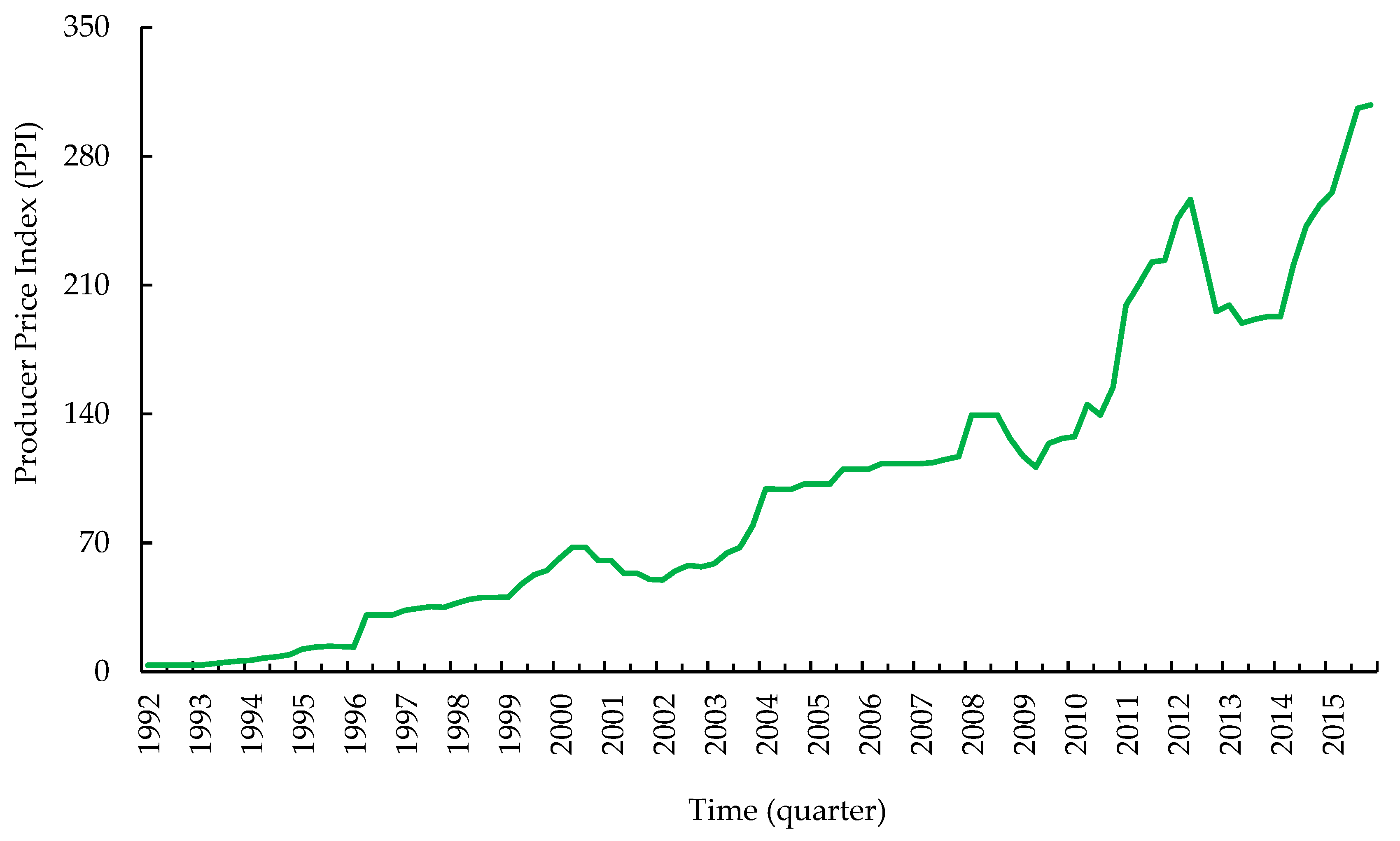
2.1. Study Area and Data Source

In the north of Iran, the Hyrcanian temperate forests, also known as Caspian temperate forests, cover an area of 1.8 million ha, vesting from the coast of the Caspian Sea to an altitude of 2800 m above sea level on the northern slopes of the Alborz Mountain belt [38,39]. Generally, these forests are mixed broadleaf and managed as uneven-aged mountain forests [40,41]. The average of standing volume is about 500 m3 ha−1, and the most valuable tree species include oriental beech (Fagus orientalis), chestnut-leaved oak (Quercus castaneifolia), common hornbeam (Carpinus betulus), Caucasian alder (Alnus subcordata), and velvet maple (Acer velutinum) [42]. Various silvicultural methods have been used to manage the Hyrcanian forests: shelter wood-cutting from 1970 to 2000, selection cutting from 2000 to 2014, and restricted cutting to damaged and fallen trees from 2016 to the present [43]. The average annual precipitation ranges from 600 mm in the east to more than 2000 mm in the western Hyrcanian temperate forests [44,45]. The data were collected from official auctions timber sale lot documents in the Azarroud Forestry Plan (36°10′ N (latitude) and 52°50′ E (longitude); located in a Mazandaran province) that occurred on the forestry plan of the roadside from 1992 to 2015. The relevant data of 592 sale lots, including sawlog and lumber prices at forest roadside, were extracted into a data set. The sawlog and lumber are timber with dimensions 2 m × 0.3 m and 2.6 m × 0.22 m × 0.14 m, respectively. Additionally, the average lumber prices are cheaper than sawlog prices because the dimension lumber is the mandatory and limited function in the conversion industry, such as veneering. In order to consider the construction activity in cities of Iran and its relationship with seasonal variations in timber prices, we used the data on the number of residential units completed by the private sector in urban areas [46].

2.2. Calculations

The average timber prices (i.e., sawlog and lumber) were calculated per season/year. Two-time series of quarterly seasonal prices (i.e., Q1 = quarter 1; Q2 = quarter 2; quarter 3 = Q3; quarter 4 = Q4) for the sawlog and lumber were obtained as dependent variables and regressed on four seasonal dummy variables as the independent variable. The inflation effect from raw data was removed using the producer price index (PPI) deflator [47] (Figure A1).

2.2.1. Unit Root Test

Unit root tests are used to identify whether time series are stationary [48]. The augmented Dickey–Fuller (ADF) unit root test was used in Eviews software (Ver. 10.0) [49,50], which is widely applied to test whether the price time series and their first (and second) differences, respectively, are stationary [48,51,52]. Since large autoregressive terms were present, the ADF test for a unit root was employed [9,53,54]. We would reject the null hypothesis of non-stationarity if the critical values were greater than ADF test statistics.

2.2.2. Multiple Linear Regression Analysis

The effect of sale seasons on timber price was analyzed using multiple linear regression in Eviews (Ver. 10.0). We considered classical econometric hypotheses such as normality of the residual, multicollinearity, serial correlation residual of regression by Jarque–Bera test, variance inflation factor (VIF), and Durbin–Watson (DW) statistic, respectively. The null hypothesis of the normality test was rejected if the p-value > 0.05. As a result, residual values of models are normally distributed. This study used VIF statistics to detect the magnitude of multicollinearity in the multiple regression analysis. If VIF was less than 2, multicollinearity is not there [55]. Finally, the DW statistic is a test for autocorrelation in the residuals from a regression analysis. If DW reported 2, the residual values of the model had no autocorrelation [56].

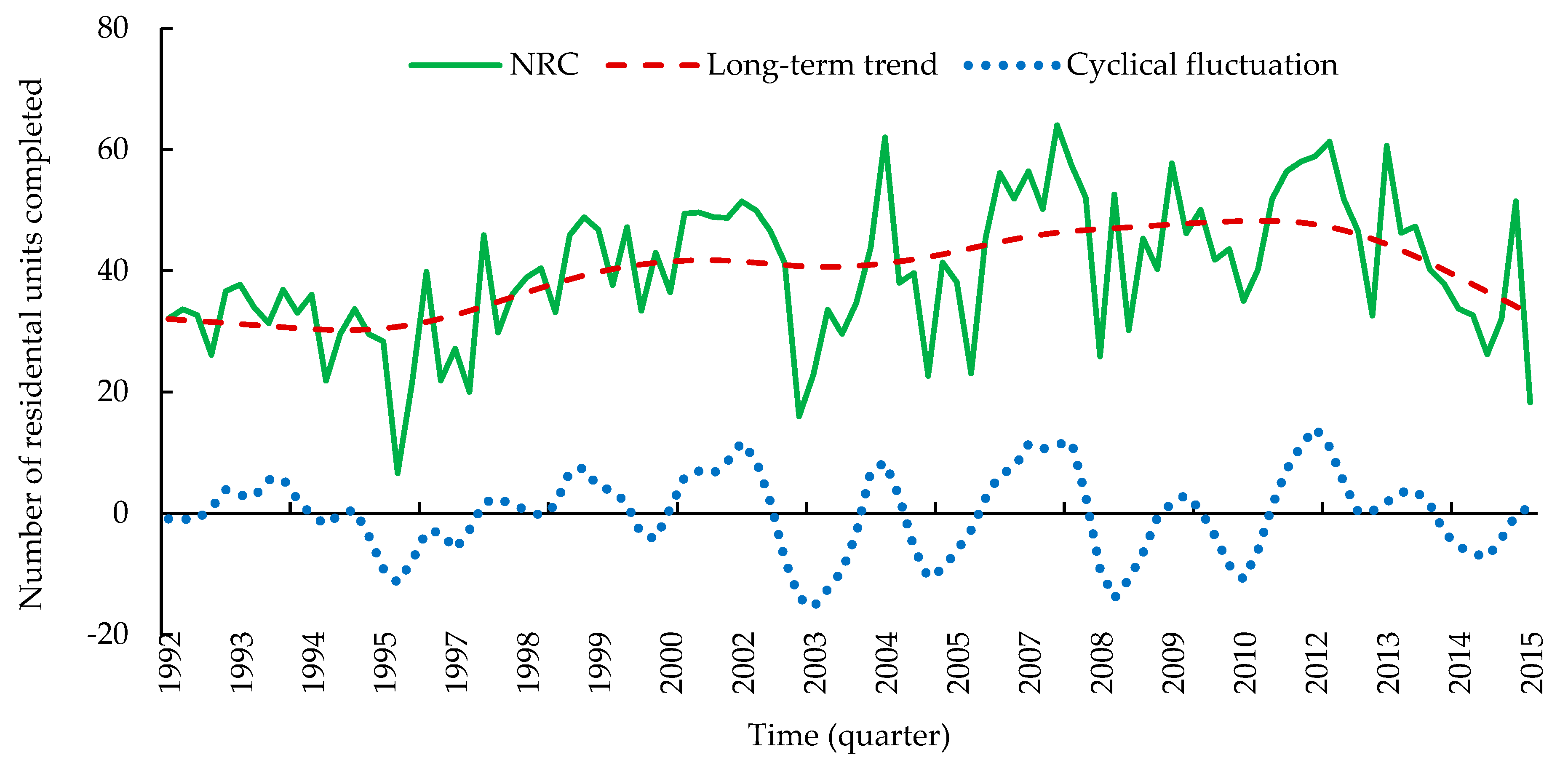
2.2.3. Decomposition of the Price Time Series

The timber price and construction activity of time series were described using a multiplicative model incorporating four components of the following form [35]:
Yt = Tt · Ct · St · It
where Yt is a timber price in period t, Tt is a long-term trend, Ct is a cyclical fluctuation, St is a seasonal fluctuation, and It is an irregular fluctuation.
Individual components of the time series were identified using the Census X11 method). Seasonality was eliminated from the initial series by dividing empirical price values by the corresponding seasonality indicators. The trend-cycle (TC) component was extracted as a Henderson moving average from the time series. Then it was decomposed into a long-term trend (T) and cyclical fluctuations (C) using the Hodrick–Prescott filter (using Gretl 2020b package) [57]. The Hodrick–Prescott filter was used to separate the cyclical component from the trend to isolate a stochastic smoothly varying trend [58,59]. In turn, irregular changes (I) were extracted by dividing the time series without the seasonal component by the trend cycle. The significance of seasonal fluctuations was estimated using the F test [57]. To determine the relative contributions of the various components to the overall price variation, the proportions of the variance of those components in the total variance were calculated for time horizons of one to four quarters and annual means.

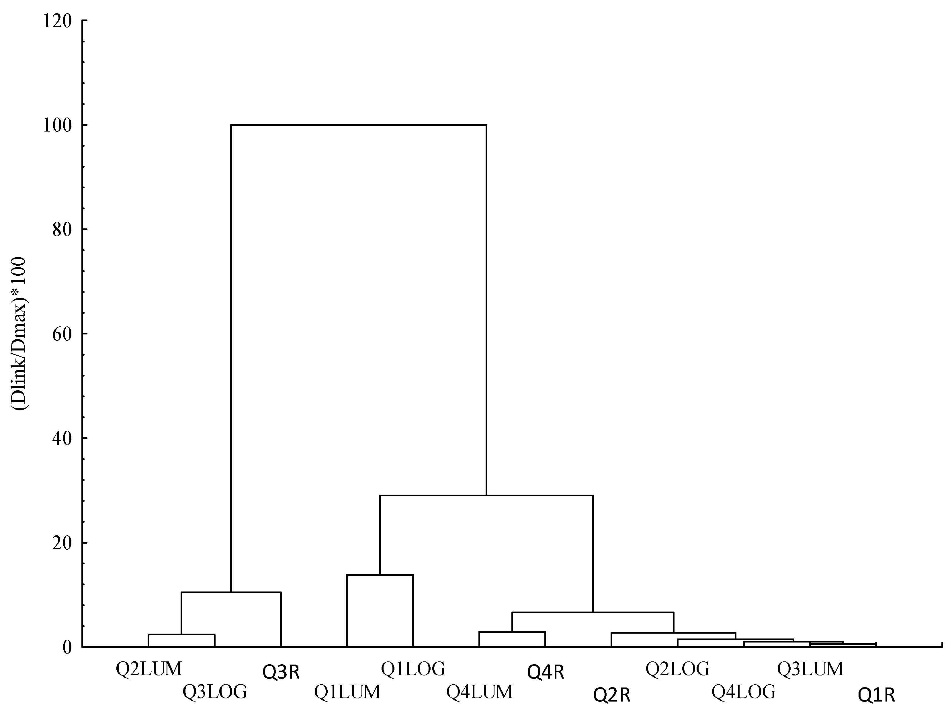
2.3. Similarity of the Seasonal Indices of Timber Price and Construction Activity

In order to consider similarity between the time series of timber price (i.e., sawlog and lumber) and construction activity, we categorized the quantitative variables in terms of seasonal indices. Therefore, we used the tree clustering method and algorithm of the complete linkage rule (squared Euclidean distances) [37,60,61].

3. Results

3.1. Descriptive Statistics

Descriptive statistics of two-time series for the sawlog and lumber of high-value species were contained in Table 1. The results showed that the sawlog price has the highest average price (140.15 US $ m−3).

3.2. ADF Test

The critical values of ADF test for two groups were −3.95 (p-value = 0.003) and −3.20 (p-value = 0.023), respectively (See Appendix B, Table A1 and Table A2). Therefore, the results of the ADF test showed that the time series of the forest products price is stationary.

3.3. The Linear Regression Parameter

Table 2 and Table 3 showed statistically significant regression analysis results at the 5% level. The estimated coefficients on the seasonal dummy variables showed that autumn and summer have a significant positive effect on sawlog and lumber prices with 36.7 US $ m−3 (with a t-statistic of 3.86 and SE of ±9.5 US $ m−3) and 17.9 US $ m−3 (with a t-statistic of 3.1 and SE of ±5.7 US $ m−3), respectively. Additionally, the results showed a significant adverse impact on a sawlog in spring with values of prices 38.8 US $ m−3. As a result, dummy variables of summer, winter, and spring do not significantly affect sawlog and lumber prices, respectively. Additionally, according to Table 3, instead of selling high-value species lumber in summer, its price has increased by 17.9 US $ m−3.
According to the VIF and Durbin–Watson statistics (Table 4), the estimated models of sawlog and lumber of high-value species have no multicollinearity and serial correlation in residuals of the model, respectively. Additionally, since the Jarque–Bera statistic is not significant at the level of 0.05, the normality assumption of residual models was accepted.

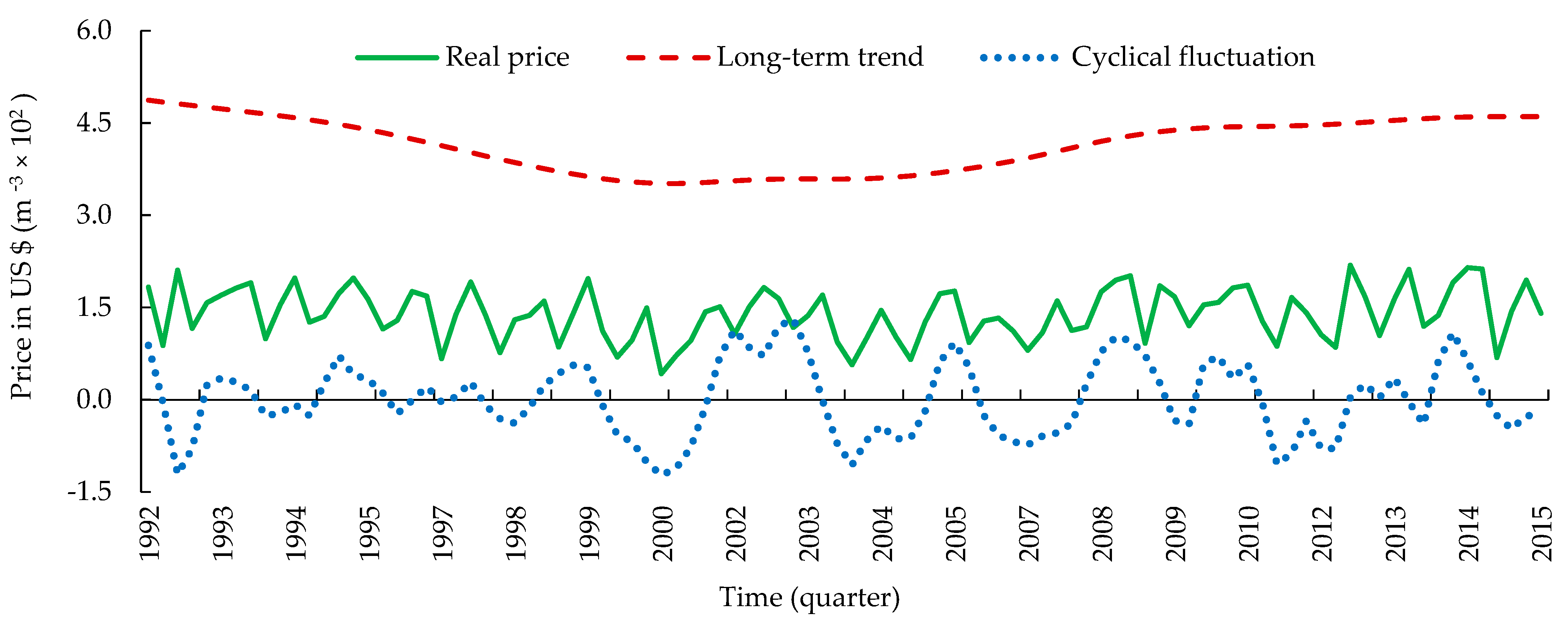
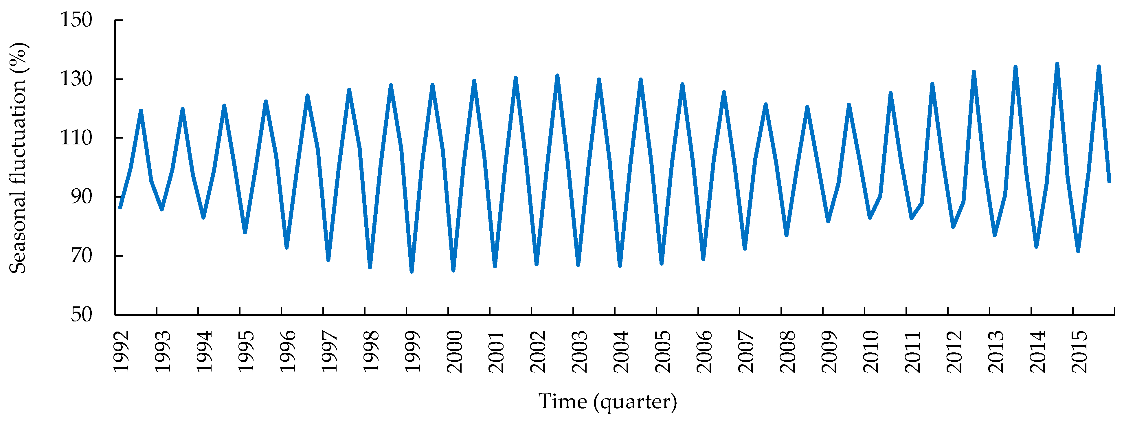
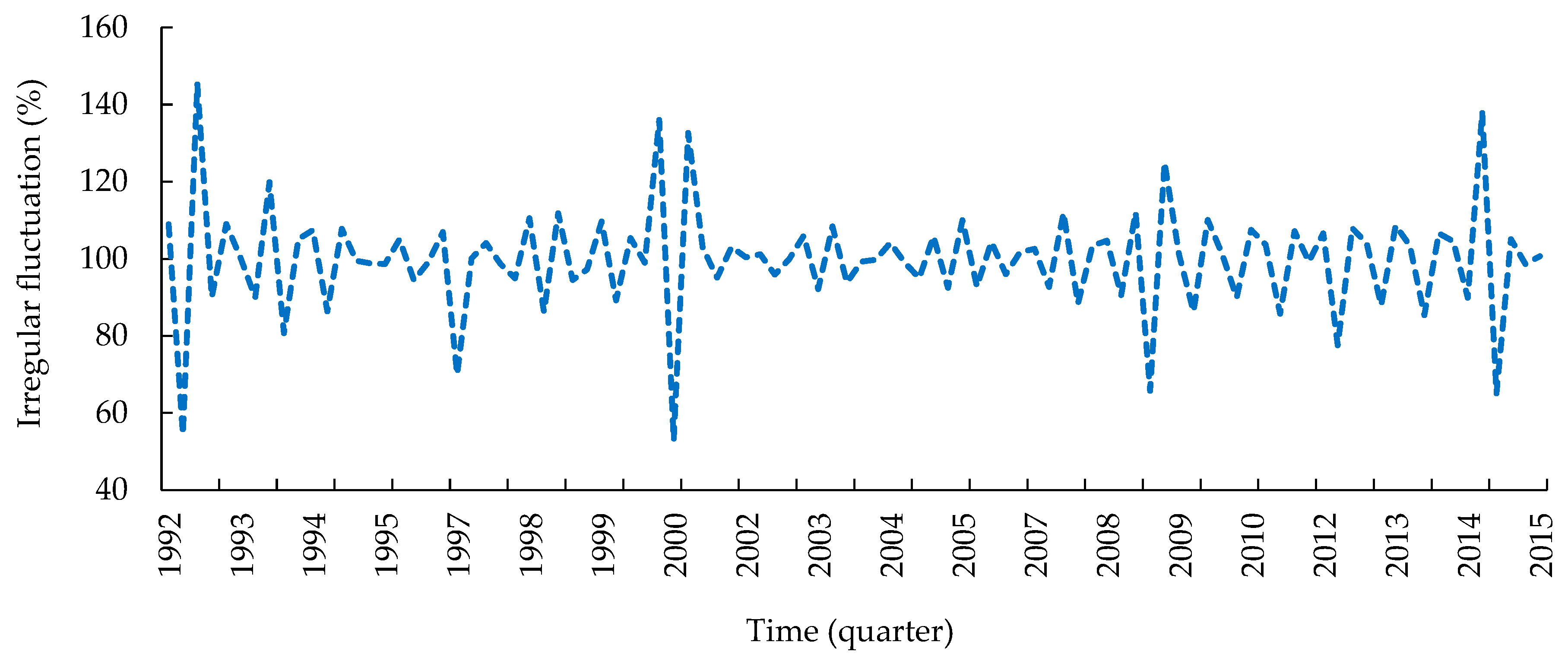
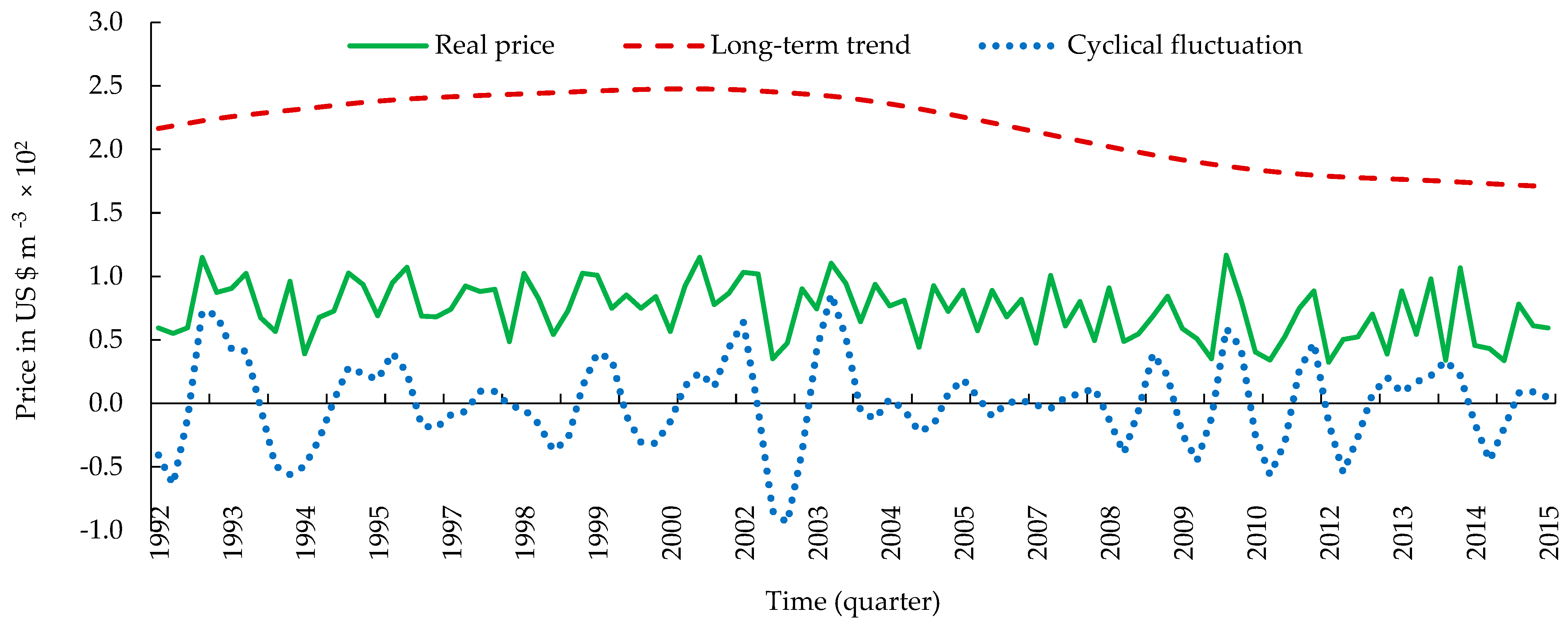
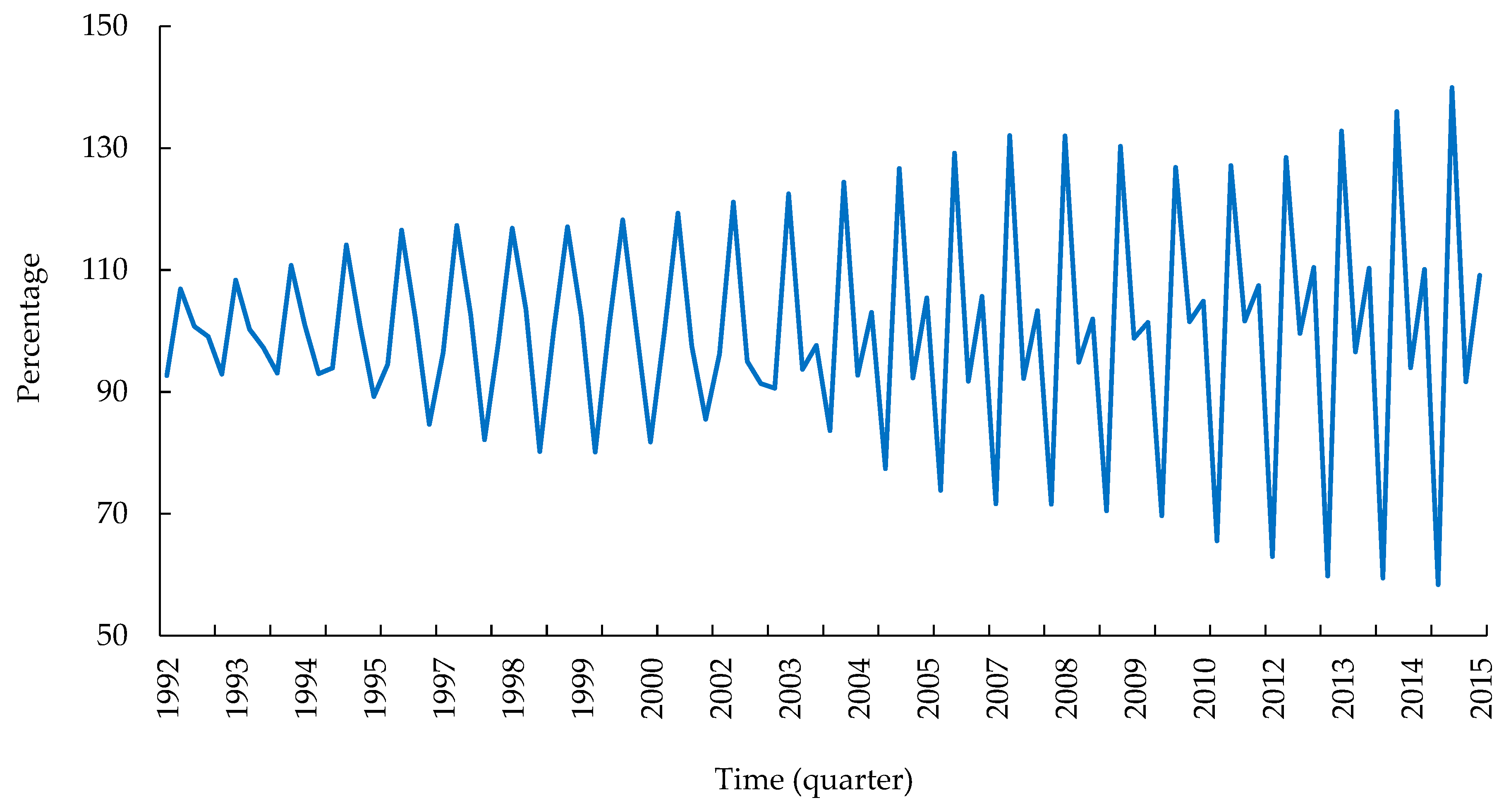
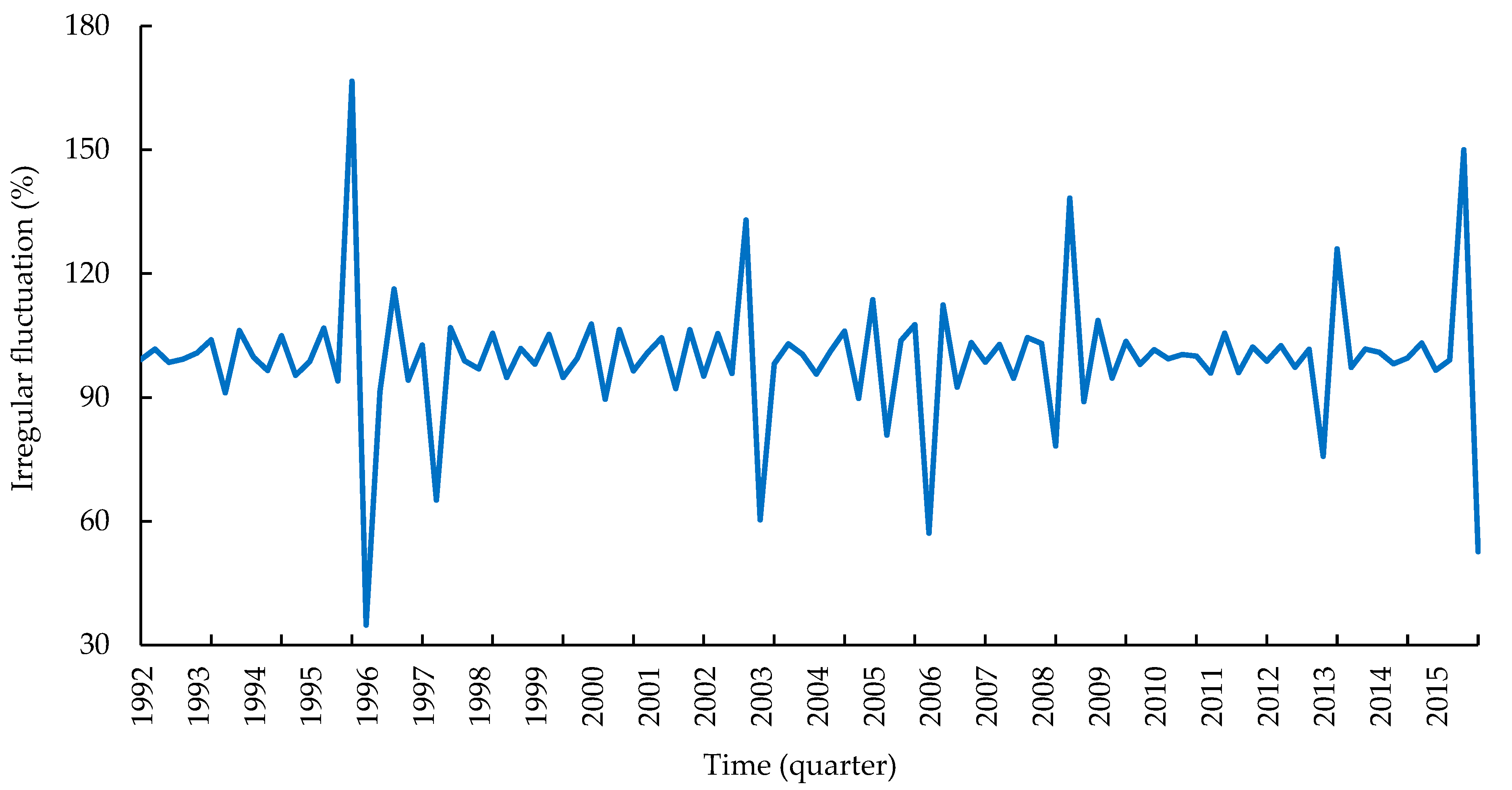
3.4. Fluctuation of Timber Price

The quarterly time series of sawlog prices decomposition revealed seasonal, cyclical, and irregular fluctuation (Figure 1, Figure 2 and Figure 3). The sawlog prices, up to 2000, were characterized by a downward trend, followed by a period of stabilization, and next to an increasing trend (Figure 1). The steady seasonality test results proved that the seasonal fluctuation of sawlog price was statistically significant (p < 0.001; F = 58.31) (Table 5), the lowest prices were in Q1, and the highest in Q3 (Figure 2). The amplitude of seasonal fluctuations in 1992 was 32.9% and gradually increased to 64% in 2002. Cyclical fluctuations varied both in the amplitude of changes and cycle duration, with three major cycles identified between 1999 and 2008. In this period, the lower inflection points of the cycle fell in Q4 2000, Q1 2004, and Q1 2007, respectively, and the upper ones in Q2 2010 and Q3 2012. The largest irregular changes (Figure 3) were found in Q2 1992 (−46%), Q4 2000 (−47%), and Q4 2014 (+38%).
Different fluctuations also characterize the lumber price (Figure 4, Figure 5 and Figure 6). The long-term trend slightly increases up to 2002, and after that slowly decreases. The seasonal fluctuations of lumber prices were statistically significant (p < 0.001, F = 21.45) (Table 6). The seasonality model changed during the study period: the highest price of lumber was in Q2 in all period, the lowest price was in Q1 up to 1994, from 1995 to 2002 it moved to Q4, and from 2003 it came back to Q1. From 2003 there were two seasonal peaks of higher lumber prices: the bigger in Q1 and the smaller in Q4.
The effects of seasonal fluctuation on overall price variation were the biggest within the one quarter, amounting 62% in both sawlog and lumber prices. Within two quarters the span increased to 70% in sawlog and decreased to 46% in lumber (Table 7). In terms of annual-average values, seasonal fluctuations explained the largest portion of price variation (48% and 39% for the sawlog and lumber, respectively), while irregular changes accounted for the smallest percentage of price variation (25%). Additionally, Table 7 shows the relative contribution of irregular, cyclic, and seasonal fluctuation in total variability of price and NRC (in percent). Similar to these results, seasonality, assuming the stability of the high cost of the sawlog and lumber was significant at the 0.001 percent level (Table 8).

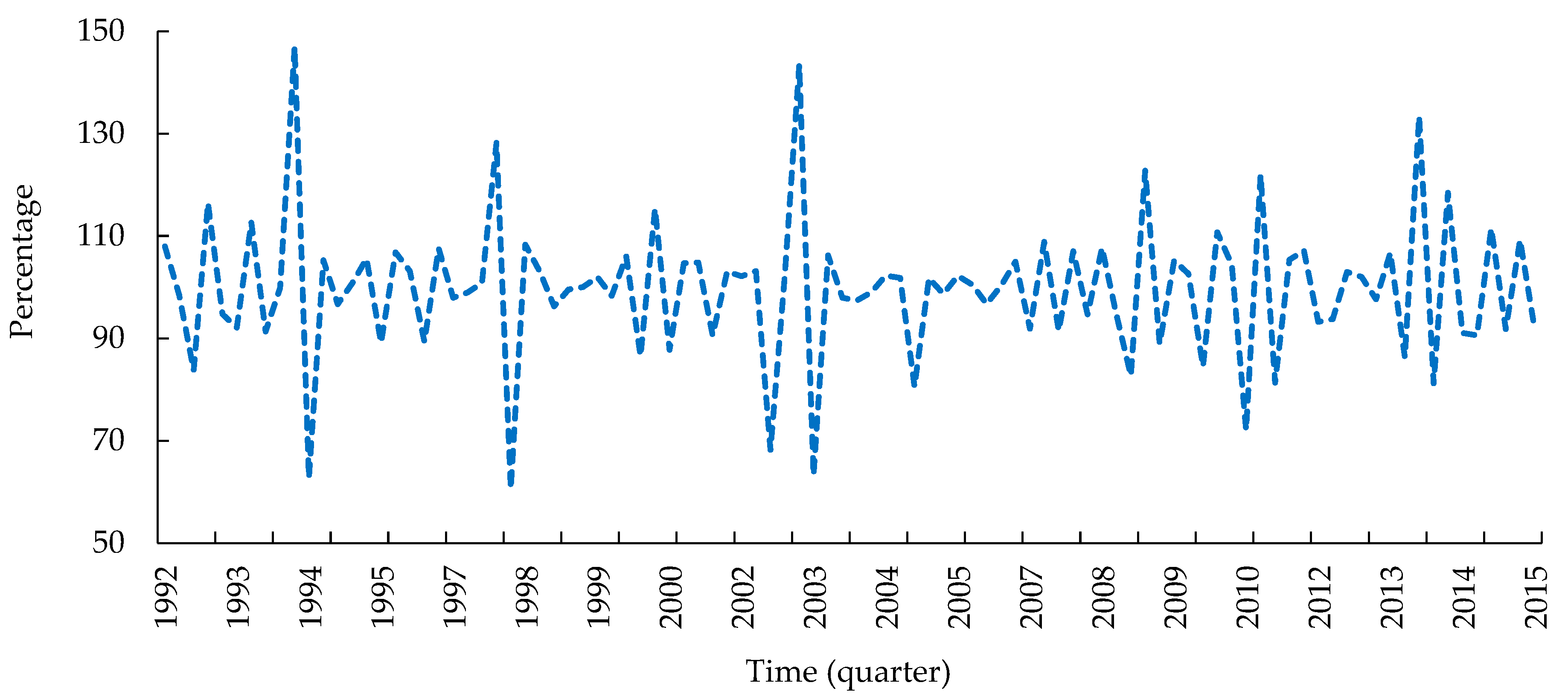
3.5. Fluctuation of the Construction Activities

Decomposition of the construction activity time series revealed this index’s seasonal, cyclical, and irregular fluctuation (Figure 7, Figure 8 and Figure 9). The number of residential units completed in long-term trend characterized relative stabilization up to 2012 followed by a period of increasing, and from 2012 it sharply decreased. As shown in Table 8, the results of the seasonality test confirmed that the seasonal fluctuation of NRC was statistically significant (p < 0.001; F = 10.08), with the lowest NRC in Q1 and the highest in Q3. Cyclical fluctuations accounted for the largest share (on average 41%) of overall NRC volatility. It is noteworthy that there is a relatively small share of seasonal fluctuations and a high share of irregular fluctuations (20% and 39%, respectively) compared to such fluctuations in sawlog prices (48% and 25% seasonal and irregular fluctuation) and lumber prices (25% and 36%, respectively).

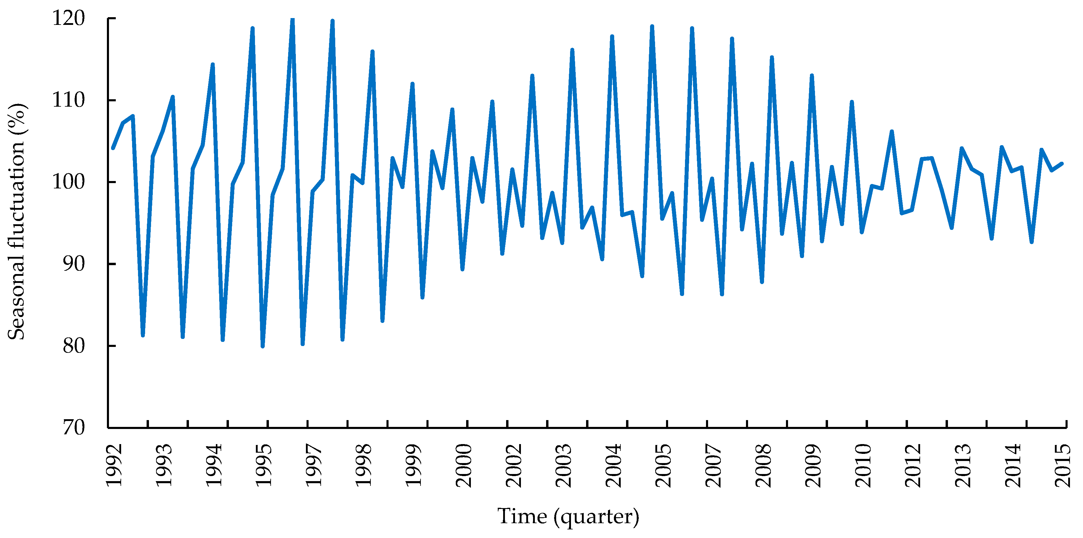
3.6. Similarity of Seasonal Index Patterns

As shown in Figure 10, Q2lum and Q3sawlog have the same pattern as Q3R. Therefore, the seasonal indices of the sawlog and lumber prices have the same pattern as the seasonal fluctuation of construction activities.

4. Discussion

Forest products’ price is well-known for fluctuations [10,62]. In general, previous studies have reported the causes of seasonal fluctuations as seasonal restrictions on harvesting, wood extraction on forest roads in winter, and the demand for timber processing factories [19,57]. As shown in literature reviews, most efforts were focused on regression analysis [30,32,63,64]. In primary and secondary industries, such as furniture, carpentry, and wooden kitchen sets, sawlog and lumber of high-value species have been used in plywood, veneering, and sawmills products. Therefore, it is expected that seasonal fluctuations in the supply and demand of timber affect its seasonal prices. The sawlog and lumber prices considered two aspects: supply and demand [36,65,66]. The results of multiple linear regression and decomposition of time series demonstrated that sale season significantly affected sawlog and lumber prices. Similar to the findings of Dahal and Mehmood [30], the study showed that spring has a significant negative effect on sawlog prices with the value of 38.8 US $ m−3. In economics, the market price reflects the interaction between supply and demand [67,68]. As the timber supply increases in the spring season (due to executing the harvesting of Hyrcanian forests), the price in autumn gave the same demand level and aggravated with low cash flow at the beginning of the year for private companies and government institutions. Additionally, the free import of timber and forest products caused a sharp fluctuation in the timber price in Iran and lowered prices for domestic wood products [69]. Therefore, it seems the imports of timber from Russia in spring decreased domestic forest products’ price due to an increase in timber supply, which corresponded with the findings of Matsushita [37] in Japan.
Viewing this from a demand perspective, the private companies encountered a lack of cash in Iran at the beginning of the New Year. Government institutions have been involved in legal consideration of construction budget rank and preparation of necessarily written agreement and then credit devotion that these occasions may cause inactivity in trade and taking orders of related industries to timber in spring, and as a result of it, the falling of forest products’ price. Seasonal adjustment analysis shows that the lumber price picks up during summer—these results matched with Leefers and Potter–Witter [16]. The most important demand field of timber is construction activities, which picks up in summer. In Iran, about 1800 Kg of timber per 100 square meters foundation of the building has been used in a door, partition, furniture, bed, etc. [70]. In this regard, factories and industries that process large-scale wood raw materials in the Mazandaran province and its vicinity increase their production capacities in summer. Therefore, competition intensifies when the raw material industry operates the most monopolies, and raw material prices rise [8]. Another factor affecting the lumber price formation is that because the forest area of the Hyrcanian forests is rugged, cutting, skidding, and transportation can only be done in the middle of spring and summer when the snow has melted, and the climatic conditions are relatively better. Actually, there may be seasonal restrictions on individual timber sales due to soil concerns, access concerns, rare/threatened/endangered species, disease concerns, and recreational conflicts [71]. Another factor that encourages summer purchases is high transport costs. These factors contribute to an increase in lumber prices, particularly in the summer. Similar to our result, a study by Daşdemir [72] in a temperate forest in Turkey showed that spring months positively affect beech sawlog prices.
Viewing this from a supply perspective, due to the lengthy process for processing sawlogs into lumber, domestic lumber supply coincides with the imports of foreign lumber in autumn and harvesting the broken tree and windthrow more in autumn [73]. This can increase lumber supply in autumn and, as a result, decrease lumber price.
Our findings (Table 2) explained that a high bid price of the sawlog in autumn corresponded to Dahal and Mehmood [30]. A lack of high-quality timber products (especially beech) from annual quota permits of forestry service in autumn and the presence of products was caused by marking 5%. This marking is related to damaged trees caused by forest utilization, the cut of annual quota permits in forestry plans, and forest roadside trees that could increase the sawlog prices of the high-value species group.
Statistics showed that the highest number of building permits in Tehran municipalities and other big cities picked up in summer and winter [46]. However, timber has been used at the ending stages of completed building construction that picks up in autumn for kitchen sets, doors, and other building decoration (thus, timber demand has appeared by a dilatory equivalent of make-completed building periods, i.e., at least 9 to 10 months). The results showed that summer has a significant positive effect on timber prices of 6.1%, respectively. Similar to our finding, Şen and Güngör [8] found summer timber prices were higher in Turkey.

5. Conclusions

The results suggest that the sale season significantly affects timber prices (sawlog and lumber). This research suggested interesting issues regarding timber sale policies and procedures. The static and dynamic analysis of the timber price shows that the price picks occur in the summer and autumn seasons. Therefore, it makes the highest income. However, our study highlights how managers of forestry plans would offer timber sale lots in the suitable seasons. Awareness about potential price variations will perhaps allow suppliers and users of sawlogs to adjust their supply and demand. Further research is needed to examine the influential factors on seasonal fluctuations of timber prices.

Author Contributions

Conceptualization, S.M.H.V. and M.M.J.; methodology, M.M.J. and J.B.; software, M.M.J., S.M.M.S. and J.B.; validation, M.M.J.; formal analysis, S.M.H.V. and M.M.J.; investigation, M.M.J.; resources, M.M.J.; data curation, S.M.H.V. and M.M.J.; writing—original draft preparation, M.M.J.; writing—review and editing, S.M.M.S., J.B. and M.V.M.; visualization, M.M.J. and S.M.M.S.; supervision, S.M.H.V. and S.M.M.S.; funding acquisition, S.M.M.S. All authors have read and agreed to the published version of the manuscript.

Funding

This research received no external funding and the APC was funded by the Department of Forest Engineering, Forest Management Planning and Terrestrial Measurements.

Institutional Review Board Statement

Not applicable.

Informed Consent Statement

Not applicable.

Data Availability Statement

The data supporting the findings of this study are available from the first and second authors, upon reasonable request.

Acknowledgments

Seyed Mohammad Moein Sadeghi’s research at the Transilvania University of Brasov, Romania, has been supported by the program entitled “Transilvania Fellowship for Postdoctoral Research/Young Researchers”.

Conflicts of Interest

The authors declare no conflict of interest.

Appendix A

The producer price index (PPI) reveals the variation of commodity and services prices supplied by the producer to the final consumer. Figure A1 shows the variations of PPI during study periods.
Figure A1. The variations of producer price index (PPI) between in study period.
Forests 13 00761 g0a1

Appendix B

The results of ADF test for sawlog and lumber prices were shown in Table A1 and Table A2, respectively.
Table A1. The results of ADF test for sawlog prices.
t-Statisticsp-Value
ADF test statistics−3.200.023
Test critical values at the 5% level−2.89-
Table A2. The results of ADF test for lumber prices.
t-Statisticsp-Value
ADF test statistics−3.950.003
Test critical values at the 5% level−2.89-

References

  1. Antonoaie, V. The Effects of the Euro Adoption on the Timber Market in Romania. Bull. Transilv. Univ. Brasov. Econ. Sci. Ser. V 2013, 6, 29–36. [Google Scholar]
  2. Gejdoš, M.; Danihelová, Z. Valuation and Timber Market in the Slovak Republic. Procedia Econ. Financ. 2015, 34, 697–703. [Google Scholar] [CrossRef]
  3. Jaunky, V.C.; Lundmark, R. Dynamics of Timber Market Integration in Sweden. Forests 2015, 6, 4617–4633. [Google Scholar] [CrossRef]
  4. Poljanec, A.; Kadunc, A. Quality and Timber Value of European Beech (Fagus sylvatica L.) Trees in the Karavanke Region. Croatian J. For. Eng. 2013, 34, 151–165. [Google Scholar]
  5. Suchomel, J.; Gejdoš, M.; Ambrušová, L.; Šulek, R. Analysis of Price Changes of Selected Roundwood Assortments in Some Central Europe Countries. J. For. Sci. 2012, 58, 483–491. [Google Scholar] [CrossRef] [Green Version]
  6. Toppinen, A.; Toivonen, R. Roundwood Market Integration in Finland: A Multi-variate Cointegration Analysis. J. For. Econ. 1998, 4, 241–265. [Google Scholar]
  7. Toppinen, A.; Viitanen, J.; Leskinen, P.; Toivonen, R. Dynamics of Roundwood Prices in Estonia, Finland and Lithuania. Balt. For. 2005, 11, 88–96. [Google Scholar]
  8. Gökhan, Ş.; Gungor, E. Determination of the Seasonal Effect on the Auction Prices of Timbers and Prediction of Future Prices. Bartın Orman Fakültesi Derg. 2018, 20, 266–277. [Google Scholar]
  9. Kożuch, A.; Banaś, J. The Dynamics of Beech Roundwood Prices in Selected Central European Markets. Forests 2020, 11, 902. [Google Scholar] [CrossRef]
  10. Banaś, J.; Utnik-Banaś, K. Evaluating a Seasonal Autoregressive Moving Average Model with an Exogenous Variable for Short-Term Timber Price Forecasting. For. Pol. Econ. 2021, 131, 102564. [Google Scholar] [CrossRef]
  11. Prestemon, J.P.; Pye, J.M.; Holmes, T.P. Temporal Aggregation and Testing for Timber Price Behavior. Nat. Resour. Model. 2004, 17, 123–162. [Google Scholar] [CrossRef]
  12. Størdal, S. Efficient Timber Pricing and Purchasing Behavior in Forest Owners’ Associations. J. For. Econ. 2004, 10, 135–147. [Google Scholar] [CrossRef]
  13. Accastello, C.; Blanc, S.; Mosso, A.; Brun, F. Assessing the Timber Value: A Case Study in the Italian Alps. For. Pol. Econ. 2018, 93, 36–44. [Google Scholar] [CrossRef]
  14. Fornea, M.; Bîrda, M.; Borz, S.A.; Popa, B.; Tomašić, Ž. Harvesting Conditions, Market Particularities or Just Economic Competition: A Romanian Case Study Regarding the Evolution of Standing Timber Contracting Rates. Šumarski List 2018, 142, 499–507. [Google Scholar]
  15. Carter, D.R.; Newman, D.H. The Impact of Reserve Prices in Sealed Bid Federal Timber Sale Auctions. For. Sci. 1998, 44, 485–495. [Google Scholar]
  16. Leefers, L.A.; Potter-Witter, K. Timber Sale Characteristics and Competition for Public Lands Stumpage: A Case Study from the Lake States. For. Sci. 2006, 52, 460–467. [Google Scholar]
  17. Rissman, A.R.; Geisler, E.; Gorby, T.; Rickenbach, M.G. “Maxed Out on Efficiency”: Logger Perceptions of Financial Challenges Facing Timber Operations. J. Sustain. For. 2022, 41, 115–133. [Google Scholar] [CrossRef]
  18. Newman, D.H.; Gilbert, C.B.; Hyde, W.F. The Optimal Forest Rotation with Evolving Prices. In Economics of Forestry; Routledge: London, UK, 2018; pp. 213–220. [Google Scholar]
  19. Zwirglmaier, K. Seasonal Influence in Determinants of Timber Supply and Demand. In Proceedings of the Managerial Economics and Accounting Conference, Hamburg, Germany, 21–23 October 2009; pp. 21–23. [Google Scholar]
  20. Conrad, J.L., IV.; Demchik, M.C.; Vokoun, M.M. Effects of Seasonal Timber Harvesting Restrictions on Procurement Practices. For. Prod. J. 2018, 68, 43–53. [Google Scholar] [CrossRef]
  21. Kolis, K.; Hiironen, J.; Ärölä, E.; Vitikainen, A. Effects of Sale-Specific Factors on Stumpage Prices in Finland. Silva Fenn. 2014, 48, 18. [Google Scholar] [CrossRef] [Green Version]
  22. Michinaka, T.; Kuboyama, H.; Tamura, K.; Oka, H.; Yamamoto, N. Forecasting Monthly Prices of Japanese Logs. Forests 2016, 7, 94. [Google Scholar] [CrossRef] [Green Version]
  23. Han, X.; Kant, S.; Xie, Y. Bidder’s Private Value Distributions in Standing Timber Auctions in the Jiangxi Province of China. Canad. J. For. Res. 2018, 48, 1441–1455. [Google Scholar] [CrossRef]
  24. Préget, R.; Waelbroeck, P. Timber Appraisal from French Public Auctions: How to set the Reserve Price When There Are Unsold Lots? In Proceedings of the International Conference of the Scandinavian Society of Forest Economics, Uppsala, Sweden, 23–26 May 2006. [Google Scholar]
  25. Puttock, G.D.; Prescott, D.M.; Meilke, K.D. Stumpage Prices in Southwestern Ontario: A Hedonic Function Approach. For. Sci. 1990, 36, 1119–1132. [Google Scholar]
  26. Li, L.; Shen, Y.; Xu, X.; Zhang, Y.; Gu, G. Stumpage Price Determination in China’s Collective Forest Region, Zhejiang as an Example. For. Pol. Econ. 2020, 117, 102215. [Google Scholar] [CrossRef]
  27. Rosen, S. Hedonic Prices and Implicit Markets: Product Differentiation in Pure Competition. J. Politic. Econ. 1974, 82, 34–55. [Google Scholar] [CrossRef]
  28. Chen, H.; He, Z.; Hong, W.; Liu, J. An Assessment of Stumpage Price and the Price Index of Chinese Fir Timber Forests in Southern China Using a Hedonic Price Model. Forests 2020, 11, 436. [Google Scholar] [CrossRef] [Green Version]
  29. Kim, H.; Cieszewski, C. The Analysis of Pine Stumpage Prices Based on Timber Sale Characteristics of the Southern United States. J. For. Environ. Sci. 2015, 31, 38–46. [Google Scholar] [CrossRef]
  30. Dahal, P.; Mehmood, S.R. Determinants of Timber Bid Prices in Arkansas. For. Prod. J. 2005, 55, 88–94. [Google Scholar]
  31. Dunn, M.A.; Dubois, M.R. Determining Econometric Relationships Between Timber Sale Notice Provisions and High Bids Received on Timber Offerings from the Alabama Department of Conservation/State Lands Division. In Proceedings of the 1999 Southern Forest Economics Workshop, Starkville, MS, USA, 18–20 April 1999; pp. 83–90. [Google Scholar]
  32. Brown, R.N.; Kilgore, M.A.; Coggins, J.S.; Blinn, C.R. The Impact of Timber-Sale Tract, Policy, and Administrative Characteristics on State Stumpage Prices: An Econometric Analysis. For. Pol. Econ. 2012, 21, 71–80. [Google Scholar] [CrossRef]
  33. Wear, D.N.; Prestemon, J.P.; Foster, M.O. US Forest Products in the Global Economy. J. Forestry 2016, 114, 483–493. [Google Scholar] [CrossRef]
  34. MacKay, D.G.; Baughman, M.J. Multiple Regression-Based Transactions Evidence Timber Appraisal for Minnesota’s State Forests. North. J. Appl. For. 1996, 13, 129–134. [Google Scholar] [CrossRef] [Green Version]
  35. Shiskin, J. The X-11 Variant of the Census Method II Seasonal Adjustment Program; US Government Printing Office: Washington, DC, USA, 1967.
  36. Reimer, J.J. An Investigation of Log Prices in the US Pacific Northwest. For. Pol. Econ. 2021, 126, 102437. [Google Scholar] [CrossRef]
  37. Matsushta, K. The Seasonal Fluctuation of the Forest Products Price (II). Mem. Fac. Agric. Kagoshima Univ. 1992, 29, 121–133. [Google Scholar]
  38. Fathizadeh, O.; Sadeghi, S.M.M.; Holder, C.D.; Su, L. Leaf Phenology Drives Spatio-Temporal Patterns of Throughfall under a Single Quercus castaneifolia CA Mey. Forests 2020, 11, 688. [Google Scholar] [CrossRef]
  39. Rahbarisisakht, S.; Moayeri, M.H.; Hayati, E.; Sadeghi, S.M.M.; Kepfer-Rojas, S.; Pahlavani, M.H.; Kappel Schmidt, I.; Borz, S.A. Changes in Soil’s Chemical and Biochemical Properties Induced by Road Geometry in the Hyrcanian Temperate Forests. Forests 2021, 12, 1805. [Google Scholar] [CrossRef]
  40. Deljouei, A.; Abdi, E.; Marcantonio, M.; Majnounian, B.; Amici, V.; Sohrabi, H. The impact of forest roads on understory plant diversity in temperate hornbeam-beech forests of Northern Iran. Environ. Monit. Assess. 2017, 189, 1–15. [Google Scholar] [CrossRef] [PubMed]
  41. Deljouei, A.; Sadeghi, S.M.M.; Abdi, E.; Bernhardt-Römermann, M.; Pascoe, E.L.; Marcantonio, M. The Impact of Road Disturbance on Vegetation and Soil Properties in a Beech Stand, Hyrcanian Forest. Eur. J. For. Res. 2018, 137, 759–770. [Google Scholar] [CrossRef]
  42. Nasiri, V.; Darvishsefat, A.A.; Arefi, H.; Griess, V.C.; Sadeghi, S.M.M.; Borz, S.A. Modeling Forest Canopy cover: A Synergistic Use of Sentinel-2, Aerial Photogrammetry Data, and Machine Learning. Remote Sens. 2022, 14, 1453. [Google Scholar] [CrossRef]
  43. Moradi, F.; Darvishsefat, A.A.; Pourrahmati, M.R.; Deljouei, A.; Borz, S.A. Estimating Aboveground Biomass in Dense Hyrcanian Forests by the Use of Sentinel-2 Data. Forests 2022, 13, 104. [Google Scholar] [CrossRef]
  44. Haghshenas, M.; Marvi Mohadjer, M.R.; Attarod, P.; Pourtahmasi, K.; Feldhaus, J.; Sadeghi, S.M.M. Climate Effect on Tree-Ring Widths of Fagus orientalis in the Caspian Forests, Northern Iran. Fore. Sci. Technol. 2016, 12, 176–182. [Google Scholar] [CrossRef] [Green Version]
  45. Attarod, P.; Kheirkhah, F.; Khalighi Sigaroodi, S.; Sadeghi, S.M.M. Sensitivity of Reference Evapotranspiration to Global Warming in the Caspian Region, North of Iran. J. Agric. Sci. Technol. 2015, 17, 869–883. [Google Scholar]
  46. Economic Time Series Database. The Number of Residential Units Completed by the Private Sector of Urban Areas. Available online: https://www.cbi.ir/page/8020.aspx (accessed on 3 December 2019).
  47. Dennis, D.F. Trends in New Hampshire Stumpage Prices: A Supply Perspective. North. J. Appl. For. 1989, 6, 189–190. [Google Scholar] [CrossRef]
  48. Fuhrmann, M.; Dißauer, C.; Strasser, C.; Schmid, E. Analysing Price Cointegration of Sawmill by-Products in the Forest-Based Sector in Austria. For. Pol. Econom. 2021, 131, 102560. [Google Scholar] [CrossRef]
  49. McCullough, B.D. Econometric Software Reliability: EViews, LIMDEP, SHAZAM and TSP; JSTOR: New York, NY, USA, 1999. [Google Scholar]
  50. Hultkrantz, L.; Andersson, L.; Mantalos, P. Stumpage Prices in Sweden 1909–2012: Testing for Non-Stationarity. J. For. Econ. 2014, 20, 33–46. [Google Scholar] [CrossRef] [Green Version]
  51. Rougieux, P.; Jonsson, R. Impacts of the FLEGT Action Plan and the EU Timber Regulation on EU Trade in Timber Product. Sustainability 2021, 13, 6030. [Google Scholar] [CrossRef]
  52. Wang, Y.; Zhang, X.; Guo, Z. Estimation of Tree Height and Aboveground Biomass of Coniferous Forests in North China Using Stereo ZY-3, Multispectral Sentinel-2, and DEM Data. Ecol. Indic. 2021, 126, 107645. [Google Scholar] [CrossRef]
  53. Assogba, N.P.; Zhang, D. The Conservation Reserve Program and Timber Prices in the Southern United States. For. Pol. Econom. 2022, 140, 102752. [Google Scholar] [CrossRef]
  54. Shook, S.R.; Plesha, N.; Nalle, D.J. Does Cointegration of Prices of North American Softwood Lumber Species Imply Nearly Perfectly Substitutable Products? Canad. J. For. Res. 2009, 39, 553–565. [Google Scholar] [CrossRef]
  55. Neter, J.; Wasserman, W. Applied Linear Statistical Models; Richard, D., Ed.; Irwin: Homewood, IL, USA, 1974. [Google Scholar]
  56. Gujarati, D.N. Basic Econometrics; Tata McGraw-Hill Education: New York, NY, USA, 2009. [Google Scholar]
  57. Banaś, J.; Kożuch, A. The Application of Time Series Decomposition for the Identification and Analysis of Fluctuations in Timber Supply and Price: A Case Study from Poland. Forests 2019, 10, 990. [Google Scholar] [CrossRef] [Green Version]
  58. Hodrick, R.J.; Prescott, E.C. Postwar US Business Cycles: An Empirical Investigation. J. Money Credit. Bank. 1997, 29, 1–16. [Google Scholar] [CrossRef]
  59. Ravn, M.O.; Uhlig, H. On Adjusting the Hodrick-Prescott Filter for the Frequency of Observations. Rev. Econ. Stat. 2002, 84, 371–380. [Google Scholar] [CrossRef] [Green Version]
  60. Matsushita, K. The Seasonal Fluctuation of the Forest Products Price (I). Mem. Fac. Agric. Kagoshima Univ. 1992, 28, 153–163. [Google Scholar]
  61. Kuuluvainen, J.; Karppinen, H.; Ovaskainen, V. Landowner Objectives and Nonindustrial Private Timber Supply. For. Sci. 1996, 42, 300–309. [Google Scholar]
  62. Buongiorno, J.; Balsiger, J. Quantitative Analysis and Forecasting of Monthly Prices of Lumber and Flooring Products. Agric. Syst. 1977, 2, 165–181. [Google Scholar] [CrossRef]
  63. Niquidet, K.; Van Kooten, G.C. Transaction Evidence Appraisal: Competition in British Columbia’s Stumpage Markets. For. Sci. 2006, 52, 451–459. [Google Scholar]
  64. Zimmermann, K.; Schuetz, T.; Weimar, H. Analysis and Modeling of Timber Storage Accumulation After Severe Storm Events in Germany. Eur. J. For. Res. 2018, 137, 463–475. [Google Scholar] [CrossRef]
  65. Devadoss, S. An Evaluation of Canadian and US Policies of Log and Lumber Markets. J. Agric. Appl. Econ. 2008, 40, 171–184. [Google Scholar] [CrossRef] [Green Version]
  66. van Kooten, G.C.; Johnston, C. Global Impacts of Russian Log Export Restrictions and the Canada—US Lumber Dispute: Modeling Trade in Logs and Lumber. For. Pol. Econ. 2014, 39, 54–66. [Google Scholar] [CrossRef]
  67. Fruteau, C.; Voelkl, B.; van Damme, E.; Noë, R. Supply and Demand Determine the Market Value of Food Providers in Wild Vervet Monkeys. Proc. Nat. Acad. Sci. USA 2009, 106, 12007–12012. [Google Scholar] [CrossRef] [Green Version]
  68. Morland, C.; Schier, F.; Janzen, N.; Weimar, H. Supply and Demand Functions for Global Wood Markets: Specification and Plausibility Testing of Econometric Models within the Global Forest Sector. For. Pol. Econ. 2018, 92, 92–105. [Google Scholar] [CrossRef]
  69. Bayatkashkoli, A.; Faezipour, M.; Azizi, M.; Gholezadeh, H. Price Index Trend of Wood and Its Products in Iran. Pajouhesh Sazandegi 2009, 21, 19–27. [Google Scholar]
  70. Saeed, A. Fundamentals of Practical Economics in Forest Management; University of Tehran Press: Tehran, Iran, 1992. [Google Scholar]
  71. Demchik, M.C.; Conrad, J.L., IV.; McFarlane, D.; Vokoun, M. Wisconsin Timber Sale Availability as Impacted by Seasonal Harvest Restrictions. For. Sci. 2018, 64, 74–81. [Google Scholar] [CrossRef]
  72. DAŞDEMİR, İ. Açık artırmalı kayın tomruk satış fiyatını etkileyen faktörler. Bartın J. Faculty For. 2008, 10, 1–12. [Google Scholar]
  73. Abdi, E.; Samdaliry, H.; Ghalandarayeshi, S.; Khoramizadeh, A.; Sohrabi, H.; Deljouei, A.; Kvist Johannsen, V.; Etemad, V. Modeling Wind-Driven Tree Mortality: The Effects of Forest Roads. Austrian J. For. Sci. 2020, 137, 1–21. [Google Scholar]
Figure 1. Decomposition of time series of sawlog price, including a real price as well as long-term trend and cyclical fluctuation.
Forests 13 00761 g001
Figure 2. Decomposition of time series of sawlog price, including seasonal fluctuation indices in Hyrcanian forest in 1992–2015.
Forests 13 00761 g002
Figure 3. Decomposition of time series of sawlog price, including irregular fluctuation indices in Hyrcanian forest in 1992–2015.
Forests 13 00761 g003
Figure 4. Decomposition of time series of lumber price, including real price as well as long-term trend and cyclical fluctuation in Hyrcanian forest in 1992–2015.
Forests 13 00761 g004
Figure 5. Decomposition of time series of lumber price, including seasonal fluctuation indices in Hyrcanian forest in 1992–2015.
Forests 13 00761 g005
Figure 6. Decomposition of time series of lumber price, including irregular fluctuation indices in Hyrcanian forest in 1992–2015.
Forests 13 00761 g006
Figure 7. Decomposition of the time series of construction activities, including the number of residential completed (NRC) by private sector in urban areas of Iran in the years 1992–2015 as well as long-term trend and cyclical fluctuation.
Forests 13 00761 g007
Figure 8. Decomposition of the time series of construction activities, including seasonal fluctuation indices in Hyrcanian forest in 1992–2015.
Forests 13 00761 g008
Figure 9. Decomposition of the time series of construction activities, including irregular fluctuation indices in Hyrcanian forest in 1992–2015.
Forests 13 00761 g009
Figure 10. Tree diagram for seasonal indices of sawlog and lumber price and number of residential units completed (NRC).
Forests 13 00761 g010
Table 1. Descriptive statistics of time series variables, including sawlog and lumber price and construction activities (number of residential units).
VariablesMinimumMaximumMeanSD (±)
High-value species sawlog price (US $ m−3)42.0219.0140.142.1
High-value species lumber price (US $ m−3)32.4116.673.522.2
Construction activities (unitless)661164,03439,90011,661
Table 2. Parameter estimation of seasonal price for high-value species sawlog (model 1).
CoefficientSE (±)t-Statisticp-ValueElasticity of Sawlog Price (%)R2
Intercept142.36.721.20.0000 *-0.41
Spring−38.89.5−4.080.0001 *−6.9
Summer−6.69.5−0.700.49 ns-
Autumn36.79.53.860.0002 *6.5
Winter2.99.90.30.77 ns-
Note: * and ns indicates significant and no significant relationships (p < 0.05), respectively.
Table 3. Parameter estimation of seasonal price for high-value species lumber (model 2).
CoefficientSE (±)t-Statisticp-ValueElasticity of Lumber Price (%)R2
Intercept72.04.117.70.000 *-0.22
Spring−10.55.7−1.80.070 ns-
Summer17.95.73.10.000 *6.1
Autumn−1.35.7−0.20.820 ns-
Winter−2.05.3−0.400.70 ns-
Note: * and ns indicates significant and no significant relationships (p < 0.05), respectively.
Table 4. Results of econometric classical hypothesis of sawlog and lumber price model.
ModelVIFDWJarque–Bera Statisticp-Value
Sawlog price model1.501.500.080.96 ns
Lumber price model1.501.691.910.38 ns
Note: ns indicate no significant relationship (p < 0.05).
Table 5. Results of F-test for the seasonality in high-value species of sawlog price (price in 100 US $ m−3).
SourceSum of SquaresDegrees of FreedomMean SquareF-Value
Between seasons40.8313.658.32 ***
Residual21.5920.2-
Total62.395--
Note: *** indicate significant relationships (p < 0.001), respectively.
Table 6. Results of F-test for seasonality in high-value species of lumber price (100 US $ m−3).
SourceSum of SquaresDegrees of FreedomMean SquareF-Value
Between seasons21.537.221.45 ***
Residual30.7920.333-
Total52.295--
Note: *** significant at the 0.001 level.
Table 7. Relative contribution of irregular, cyclic, and seasonal fluctuation in total variability of timber price and number of residential units completed (NRC).
Span in Quarters (Q)SawlogLumberNRC
Irregular
(%)
Cyclic
(%)
Seasonal
(%)
Irregular
(%)
Cyclic
(%)
Seasonal
(%)
Irregular
(%)
Cyclic
(%)
Seasonal
(%)
132662271162571231
2151570213446383923
3152461143749294724
4386203961033660
Average252748253639394120
Table 8. Results of F-test for seasonality in number of residential units completed (NRC) of time series.
SourceSum of SquaresDegrees of FreedomMean SquareF-Value
Between seasons8.532.8010.08 ***
Residual25.8920.28-
Total34.395--
Denote: *** significant at the 0.001 level.
Publisher’s Note: MDPI stays neutral with regard to jurisdictional claims in published maps and institutional affiliations.

