Article

Threshold Responses of Canopy Cover and Tree Growth to Drought and Siberian silk Moth Outbreak in Southern Taiga Picea obovata Forests

by
Jesús Julio Camarero
1,*,
Tatiana A. Shestakova
2 and
Manuel Pizarro
1
1
Instituto Pirenaico de Ecología (CSIC), Apdo. 202, 50192 Zaragoza, Spain
2
Woodwell Climate Research Center, 149 Woods Hole Road, Falmouth, MA 02540, USA
*
Author to whom correspondence should be addressed.
Submission received: 8 April 2022 / Revised: 29 April 2022 / Accepted: 13 May 2022 / Published: 16 May 2022

Abstract

:
The consecutive occurrence of drought and insect outbreaks could lead to cumulative, negative impacts on boreal forest productivity. To disentangle how both stressors affected productivity, we compared changes in tree canopy cover and radial growth after a severe outbreak in Siberian spruce (Picea obovata) southern taiga forests. Specifically, we studied the impacts of the 2012 severe drought followed by a Siberian silk moth (Dendrolimus sibiricus, hereafter SSM) outbreak, which started in 2016, on spruce forests by comparing one non-defoliated site and two, nearby fully defoliated sites, using remote sensing and tree-ring data. The SSM outbreak caused total defoliation and death of trees in the infested stands. We found a sharp drop (−32%) in the normalized difference infrared index and reduced radial growth in the defoliated sites in 2018. The growth reduction due to the 2012 drought was −37%, whereas it dropped to 4% of pre-outbreak growth in 2018. Tree growth was constrained by warm and dry conditions from June to July, but such a negative effect of summer water shortage was more pronounced in the defoliated sites than in the non-defoliated site. This suggests a predisposition of sites where trees show a higher growth responsivity to drought to SSM-outbreak defoliation. Insect defoliation and drought differently impacted taiga forest productivity since tree cover dropped due to the SSM outbreak, whereas tree growth was reduced either by summer drought or by the SSM outbreak. The impacts of abiotic and biotic stressors on boreal forests could be disentangled by combining measures or proxies of canopy cover and radial growth which also allow the investigation of drought sensitivity predisposes to insect damage.

1. Introduction

Unprecedented changes in the spatial and temporal patterns of abiotic and biotic stressors such as drought and insect herbivores could threaten boreal forest health [1]. In boreal forests, rapid climate warming may intensify drought stress and make insect outbreaks and defoliations more severe [2,3,4,5]. For instance, the last Siberian silk moth (Dendrolimus sibiricus Tschetv., hereafter abbreviated SSM) outbreak caused defoliation and conifer mortality across ca. 800,000 ha from 2015 to 2017 in Russian boreal forests [6,7]. In the warm 1950s, about 4000.000 ha of taiga forests were affected in Central Siberia causing widespread stand mortality [8,9]. These data evidence the role played by SSM as a major defoliator of Siberian taiga which may be considered the most destructive pest of conifers in continental Asia [10]. In addition, drought reduces boreal forest productivity, decreasing growth, impairing vitality by making trees vulnerable to other stressors, and alters morphological and physiological traits including hydraulic conductivity and xylem anatomy [1,11]. However, it is still unknown how drought and SSM outbreaks affect tree cover and growth despite the fact that both disturbances can interact and reduce forest productivity.
Dry and warm conditions in the 2–3 years prior to the SSM outbreak favor the development of SSM larvae leading to severe defoliation [2,6,12]. Warmer spring conditions in the middle and southern Siberian taiga [13,14] have enhanced SSM outbreaks’ severity, frequency and extent [15], but they could also lead to growing-season water deficit. More frequent defoliations due to SSM outbreaks could synergistically interact with increased aridity and negatively impact forests [16]. For instance, abrupt changes or shifts in forest cover, productivity or tree growth could be expected in response to successive, severe disturbances such as droughts or insect outbreaks [17], but not to frequent moderate disturbances [18]. It is still understudied how drought followed by SSM outbreak would reduce forest cover and tree radial growth.
Vegetation indices combined with long climate and tree growth series may be used to define early warning signals of SSM outbreaks, to detect shifts in forest cover or greenness and to establish mitigation measures of defoliation damage. Dead and damaged stands affected by SSM outbreaks exhibit characteristic spectral signatures with low values of normalized difference infrared index (NDII) as [12] showed. The NDII and similar vegetation indices were used to detect patches of defoliated and dead trees in other temperate and boreal forest types [19,20], thus justifying its value to assess the impacts of SSM outbreaks on forest cover.
Long-term climate data and tree-ring records could be used to characterize growth responses to water shortage and SSM outbreaks. Shifts in climate conditions or tree growth should also be investigated to detect changes in forest productivity making some stands more sensitive to SSM impacts. Stands where growth is constrained by water availability could be more severely impacted by subsequent SSM outbreak because water shortage makes trees more vulnerable to insect defoliation [21].
Here, we test these ideas by investigating a SSM outbreak which affected Siberian spruce (Picea obovata) stands near Tomsk, Western Siberia (Russia), and started in 2016. We compared radial growth in defoliated vs. nearby non-defoliated stands using a dendroecological approach. We aimed to fulfill the following objectives: (i) to quantify the impact of SSM defoliation on tree cover by using the NDII and (ii) to evaluate the growth changes and responses to climate and drought before and after the outbreak. We also used a regime shift analysis based on sequential t-tests [22] to detect abrupt changes in NDII and tree growth before or after the SSM outbreak. Since the study SSM outbreak occurred after the 2012 summer heat wave and dry spell, which negatively impacted Siberian forests triggering, for instance, many wildfires (e.g., [23]), we hypothesize that both SSM defoliation and drought interacted leading to a marked loss in tree cover and radial growth reduction due to cumulative stress. Explicitly, we expect that: (i) the SSM outbreak caused both a decrease in tree cover (NDII) due to stand defoliation and radial growth, (ii) drought caused a reduction in growth but a lower decrease in tree cover as compared to the SSM outbreak and (iii) stands more responsive to drought were prone to be more impacted by the subsequent SSM outbreak. The most novel aspect of this study is the combination of spectral information (NDII) and tree growth data to disentangle how defoliation caused by insect outbreaks and drought differently impact boreal forest productivity.

2. Materials and Methods

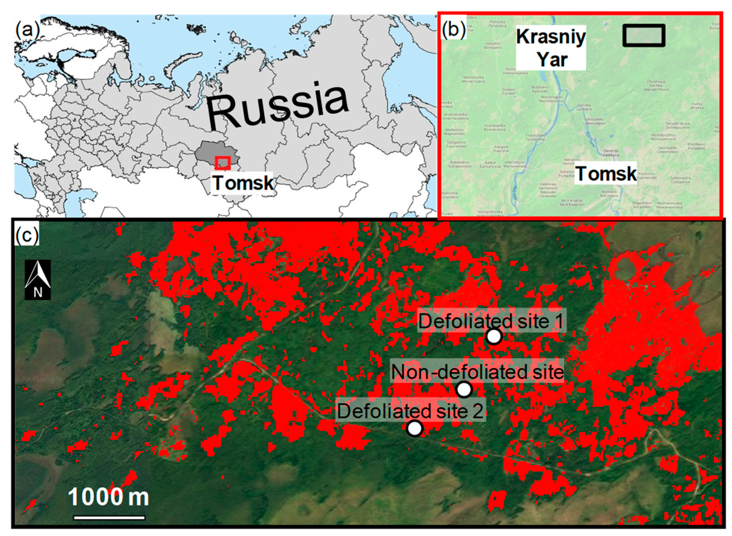
2.1. Study Sites and Species

We sampled three stands (two severely defoliated stands—hereafter D1 and D2 sites—and a nearby non-defoliated stand—hereafter ND site) located near Krasniy Yar village (Tomsk oblast), Western Siberia, in late July 2019 (Table 1, Figure 1). Sampled stands were selected based on local reports of forest technicians. The D1 and D2 sites were located on relatively flat conditions (slope 0–2°), whereas the ND site was located on a steeper slope (10–15°).
Long-term monthly climate data were obtained from the Tomsk station (56°25′48″ N, 84°58′12″ E, 137 m a.s.l.; period 1891–2019) retrieved from the Global Historical Climatology Network [25]. Average annual temperature was 0.2 °C, with January and July being the coldest (−18.5 °C) and warmest (18.7 °C) months, respectively (Figure S1). Average annual precipitation was 530 mm and mainly fell from June to August. The period with negative climate water balance started in July and ended in September (Figure S1). The long-term average snow season lasted 178 days and the mean snow depth was 0.7 m in winter.
The study sites are dominated by Siberian spruce (Picea obovata Ledeb.), Siberian pine (Pinus sibirica Du Tour) and Scots pine (Pinus sylvestris L.). Other less abundant tree species were silver birch (Betula pubescens Ehrh.) and rowan (Sorbus aucuparia L). The understory is dominated by Vaccinium and Sphagnum spp., which are found mainly in drier and wetter (peatlands) sites, respectively. In the study area, large wildfires were reported to affect Scots pine forests in the 1910s, 1950s, 1970s, 1980s, 1990s, 2000s and 2010s [23]; however, the study stands did not show charcoal or scarred trees. A few stumps were also observed in sampled stands suggesting past logging activities.
The geological substrates of the region are mainly Mesozoic-Cenozoic sedimentary rocks including clays, sandstones, and marls. Soils are of mineral type, oligotrophic and acid [23].
The study SSM outbreak started in 2016 according to local forest managers (see also [26]). In the defoliated stands, most trees were dead and completely defoliated. Defoliation affected “black taiga” conifers including P. obovata Ledeb., P. sibirica and P. sylvestris. The SSM is a lepidopteran which mainly defoliates Siberian spruce and pine by feeding on needles during spring and summer [12]. The SSM larvae emerge from the shallow soil layer from late April to early May when warm, and often dry, conditions are observed [2,27]. Temperature fluctuations, including autumn freeze–thaw cycles, are lethal to the SSM larvae which overwinter under sub-zero temperatures [28]. SSM population density peaks 3–5 years after the outbreak start and then rapidly declines. Each SSM outbreak lasts on average up to 10 years and mainly affecting low-elevation stands situated on sites with gentle slopes [29,30].
The SSM outbreaks cause defoliation of conifer seedlings and saplings, and lead to complete mortality of the overstory. These outbreaks can lead to important economic losses due to reduced timber production and positively feedback on fire occurrence by producing dead trees and fuel [31], promoting the spread of secondary pests such as bark beetles [12] or accelerating succession [32].

2.2. Field Sampling

We only sampled spruce trees, which comprised most (>90%) of the basal area of each stand. In the defoliated stands, only fully defoliated (90–100% defoliation) and recently dead, mature trees were sampled, whereas in the non-defoliated stand partially defoliated, surviving mature trees (0–15% defoliation) were sampled. Defoliated stands were fully covered by silk produced by the moth and sampled trees showed abundant resin pockets in their stems. We selected from 17 to 18 dominant and codominant trees at each site (Table 2). In the field, diameter at breast height (DBH) was measured and two cores were extracted per tree at 1.3 m using an increment borer.

2.3. Tree-Ring Data Processing

In the laboratory, cores were air-dried, glued onto wooden mounts and polished with a series of successively finer sand-paper grits until ring boundaries were clearly visible [33]. All samples were visually cross-dated using marker years based on consistently narrow rings such as the 1963 and 2012 rings. Tree-ring widths (TRW) were measured to a resolution of 0.01 mm using a LINTAB measuring device (F. Rinn, Heidelberg, Germany). Cross-dating was checked using the COFECHA software [34]. To estimate tree age at 1.3 m, we fitted templates of concentric rings to the innermost curved rings in those cores without pith. This allowed the estimation of the missing distance to the theoretical center of the stem and the guessing of the number of missing rings [35].
To calculate climate–growth relationships, we removed age-, disturbance- or size-related influences on tree-ring width through detrending [33]. Individual tree-ring width series were detrended using a cubic smoothing spline with a 50% frequency response cutoff at 2/3 length of series. Then, autoregressive models were applied to each detrended series to remove the first-order autocorrelation so as to obtain residual or pre-whitened ring-width index chronologies. These residual series were averaged by using a bi-weight robust mean to develop site-level chronologies for the three study sites. Detrending and dendrochronological statistics of raw ring-width series and residual indexed series were calculated using the dplR package [36] in R [37].
We calculated the first-order autocorrelation (AR1) of ring-width series to measure the persistence in growth and the mean sensitivity (MSx), which is the relative change in width between consecutive rings of indexed, non-prewhitened data [33]. We also obtained the mean inter-series correlation (rbar), which is based on the correlation between indexed series, and measures the whitin-site replication of the chronologies and the growth coherence among trees [38]. These variables were calculated over the common and best-replicated period 1947–2019.
Climate–growth relationships were assessed by calculating Pearson correlations between the residual chronologies and monthly or seasonal climate variables (mean temperature, total precipitation) considering the period 1950–2016, i.e., excluding the post-defoliation period (2017–2019). The window of analysis spanned from the previous to the current September. In addition, we also calculated relationships between growth rates and the standardized precipitation–evapotranspiration index (SPEI) multiscalar drought index [39] considering the same period of 1950–2016. The SPEI quantifies drought length and severity at multiple temporal scales according to the difference between the atmospheric evaporative demand and precipitation. Negative values of the SPEI indicate water scarcity with values below −1.5 usually indicating severe drought. The SPEI was calculated for 1- to 24-month temporal scales using the Tomsk climate data and the R package SPEI [40]. Climate–growth relationships were assessed using the R package treeclim [41].

2.4. Remote Sensing Data

We used two types of remote sensing information, the normalized difference infrared index (NDII) between 2000 and 2021 and estimates of forest cover loss between 2000 and 2019 based on Global Forest Change data [24]. We selected these two periods to consider remote sensing information obtained before and after the SSM outbreak. Both datasets were derived from Landsat images taken at 30 m resolution in a grid delimited by coordinates 84°42′–84°43′ E and 57°08′–57°09′ N (Table 1).
To calculate the NDII, we considered 628 scenes (16-day averaged composites) taken at the same dates on the three study sites and applied radiometric and topographic corrections using the USGS GMTED2010 digital elevation model [42]. Lastly, we carried out harmonizing from Landsat ETM+ surface reflectance to Landsat 8 OLI surface reflectance series [43]. We considered 50 m buffer areas around each site to quantify NDII. These calculations were carried out using the Google Earth Engine platform (https://earthengine.google.com, accessed on 11 January 2022).
According to [12], the NDII distinguishes dead and damaged stands after SSM outbreaks (usually showing NDII in the range 0.0–0.25) from undamaged stands (with NDII ranging 0.25 to 0.45). The NDII is defined as:
NDII = (NIR − SWIR1)/(NIR + SWIR1)
where NIR and SWIR1 are signatures in the near-infrared (851–879 nm) and shortwave infrared (1566–1651 nm) channels, respectively [44].
Next, we used the data on global changes in forest cover available at https://glad.earthengine.app/view/global-forest-change, accessed on 12 January 2022 [24]. We considered the variable of forest cover loss from 2000 to 2019 in the study area, which was defined as a stand-replacement disturbance, or a change from a forest to non-forest state. These authors [24] estimated cover loss from a set of quality assessment-passed growing season observations obtained from Landsat imagery.

2.5. Statistical Analyses

We used robust Mann–Whitney U tests to detect differences between study sites in terms of tree growth, NDII and tree responses to climate variables. In this case, the Mann–Whitney U test can be considered as the non-parametric alternative to t-tests.
To detect regime shifts in the NDII (period 2000–2021) and tree-ring width (period 1950–2019) series, we used sequential t-test analysis [22,45,46]. Briefly, a regime shift index is calculated by comparing change points in time series using a predefined running window. We selected a cutoff length of 1/7 of the series’ lengths (threshold in the Rodionov’s algorithm below which the detection of the regime shifts becomes increasingly unlikely) and a 0.05 significance level. We decided using a long cut-off to avoid false shift detections (cf. [47]). To perform these analyses, we used the open “Shift detection” Ms-Excel® template ver. 6.2.1 (available at https://sites.google.com/view/regime-shift-test; accessed on 14 January 2022).

3. Results

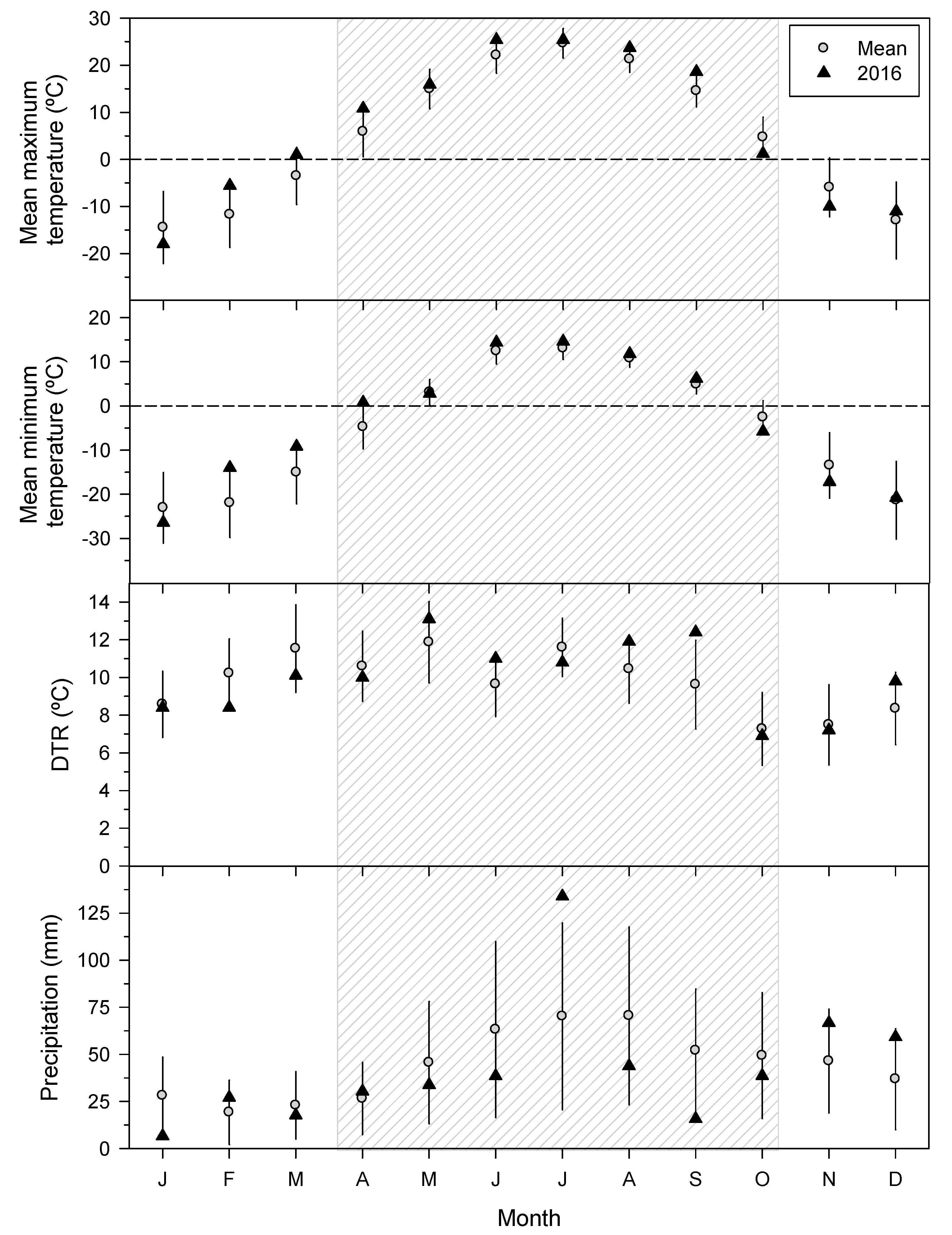
3.1. Climatic Conditions Prior to the SSM Outbreak

The 2-month July SPEI in 2012 was −2.98 and corresponded to extremely warm and dry conditions (Figure S2). June to July precipitation (38 mm) in 2012 was ca. 3.5 times lower than the long-term average (132 mm; Figure S2). The climatic conditions during 2016, when the SSM outbreaks started, were characterized by high February to April temperatures and a low diurnal thermal range in February followed by a high diurnal thermal range in August–September (Figure 2). Precipitation was low in June, August and, particularly, September, but very high in July. Monthly climatic anomalies with respect to the 1981–2010 climate averages confirmed these results for 2016 and highlighted the high minimum temperatures in February–April, the elevated diurnal temperature in August–September and the peak of July precipitation (Figure S3). They also revealed very warm conditions and a reduced diurnal thermal range during the cold season of 2013–2014 (especially November–December and March).

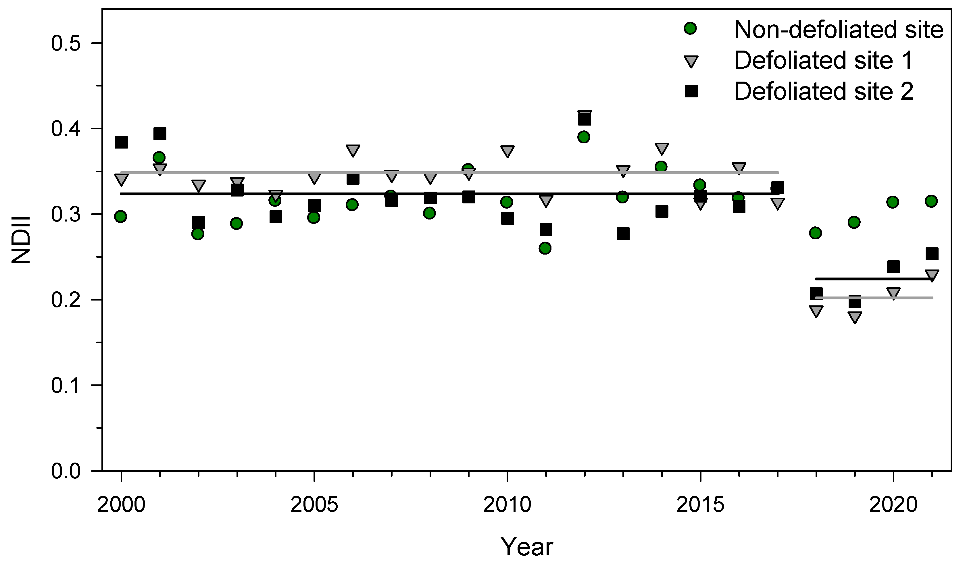
3.2. NDII Changes Due to SSM Defoliation and Drought

From 2000 to 2017, the NDII of the D1 site was significantly (U = 73, p = 0.005) higher (mean NDII ± SE = 0.35 ± 0.01) than that of the ND (0.31 ± 0.01) and D2 sites (0.32 ± 0.01). In 2018, we detected a significant (p < 0.001) regime shift index in the NDII series of the two defoliated stands corresponding to a sharp drop in NDII (Figure 3). From 2018 to 2021, the NDII of D1 (0.20 ± 0.01) and D2 (0.22 ± 0.01) sites was significantly (U = 71, p = 0.03) lower than in the ND site (0.30 ± 0.01). In 2012, the NDII increased (the mean value across sites was 0.41), reaching the maximum value of the period 2000–2021 at each site.

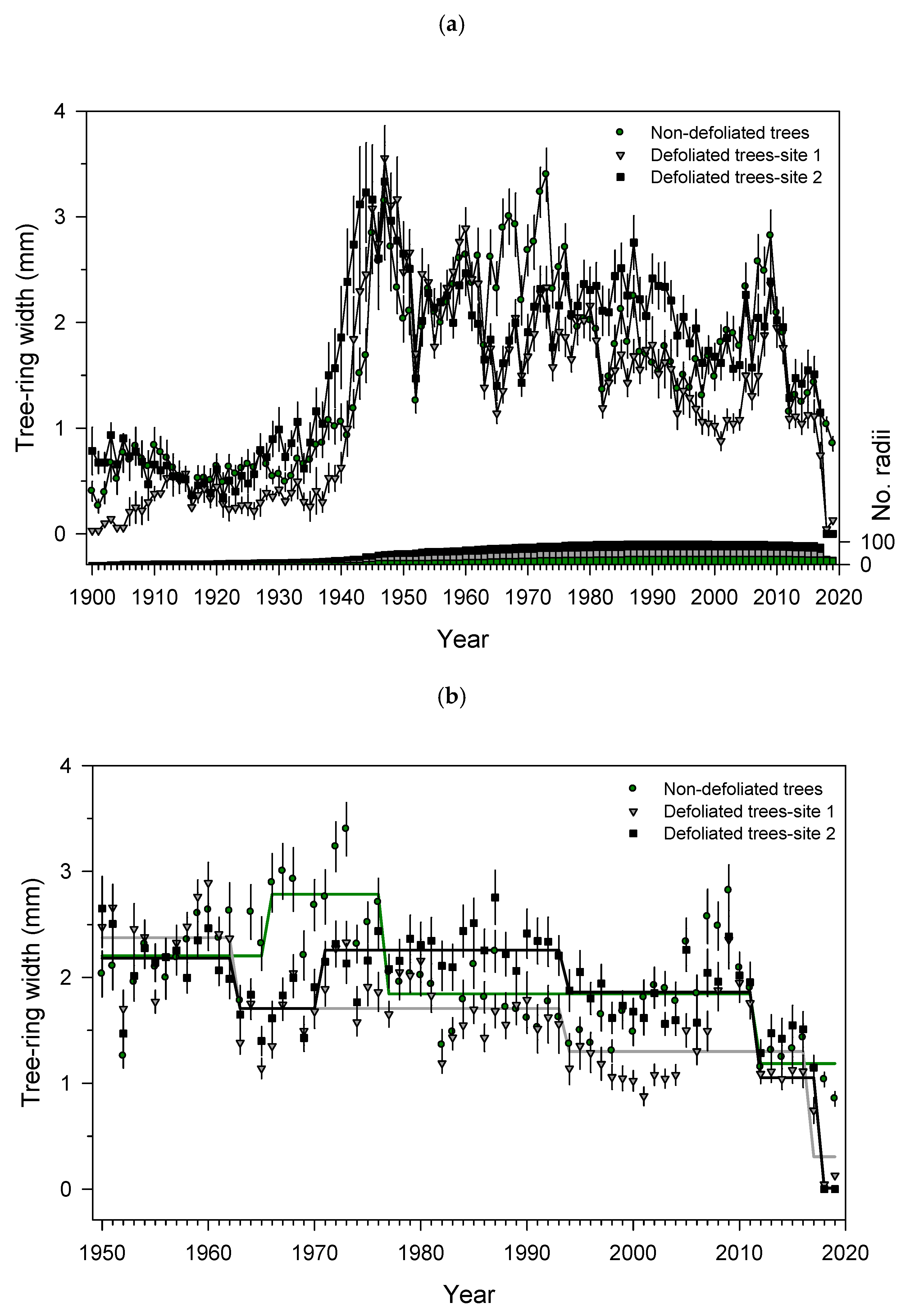
3.3. Growth Patterns

The growth releases observed in the mid-1940s were probably caused by logging (Figure 4a), suggested by the presence of stumps. The impact of these local disturbances was similar at the three study sites since there was neither a difference in tree diameter (U = 224, p = 0.16; Table 1) nor in age at 1.3 m (U = 292, p = 0.93; Table 2) between the sites.
In 2017, after the SSM outbreak started, the mean growth reduction in defoliated sites was −28.7% (vs. −22.2% for ND), whereas it dropped to −95.7% in 2018 (vs. −9.2% for ND) and −71.8% in 2019 (vs. −17.6% for ND) (Figure 4). In comparison, the growth reduction one year after the 2012 drought was −37.2% on average, with a small variability among sites (ND site, −39.4%; D1 site, −38.1%, D2 site, −34.2%; Figure 4). Growth recovered in 2014 with a mean growth change of 10.1%.
We detected eleven significant (p < 0.01) regime shift index values of tree growth in the three stands, and nine of them were negative, i.e., corresponded to growth reductions (Figure 4b). The negative shift after the 2016 outbreak was the strongest growth reduction in the two defoliated sites, and it was followed by a growth decline in the 2012 severe drought (Figure S2), which was not detected in the D1 site (Figure 4b).
If the regime shift analysis was carried out with either shorter (5 years) or longer (15 years) cutoffs, the 2012 negative shift was detected in the three study sites (Figure S5). Another negative shift was detected in 1963 in the two defoliated sites, also corresponding to dry conditions (Figure S2). In the ND site, a positive shift was found in 1966 followed by a negative shift in 1977.

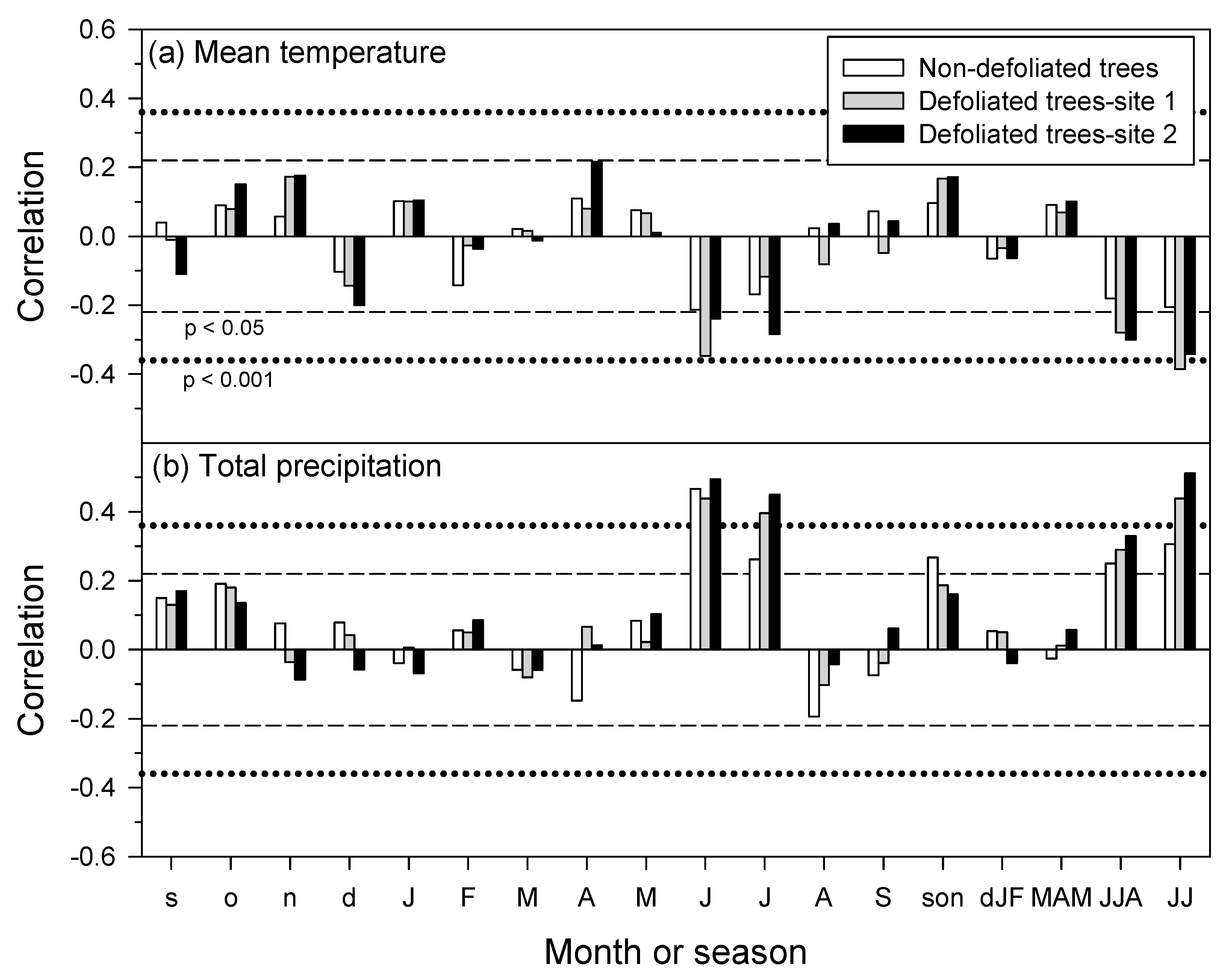
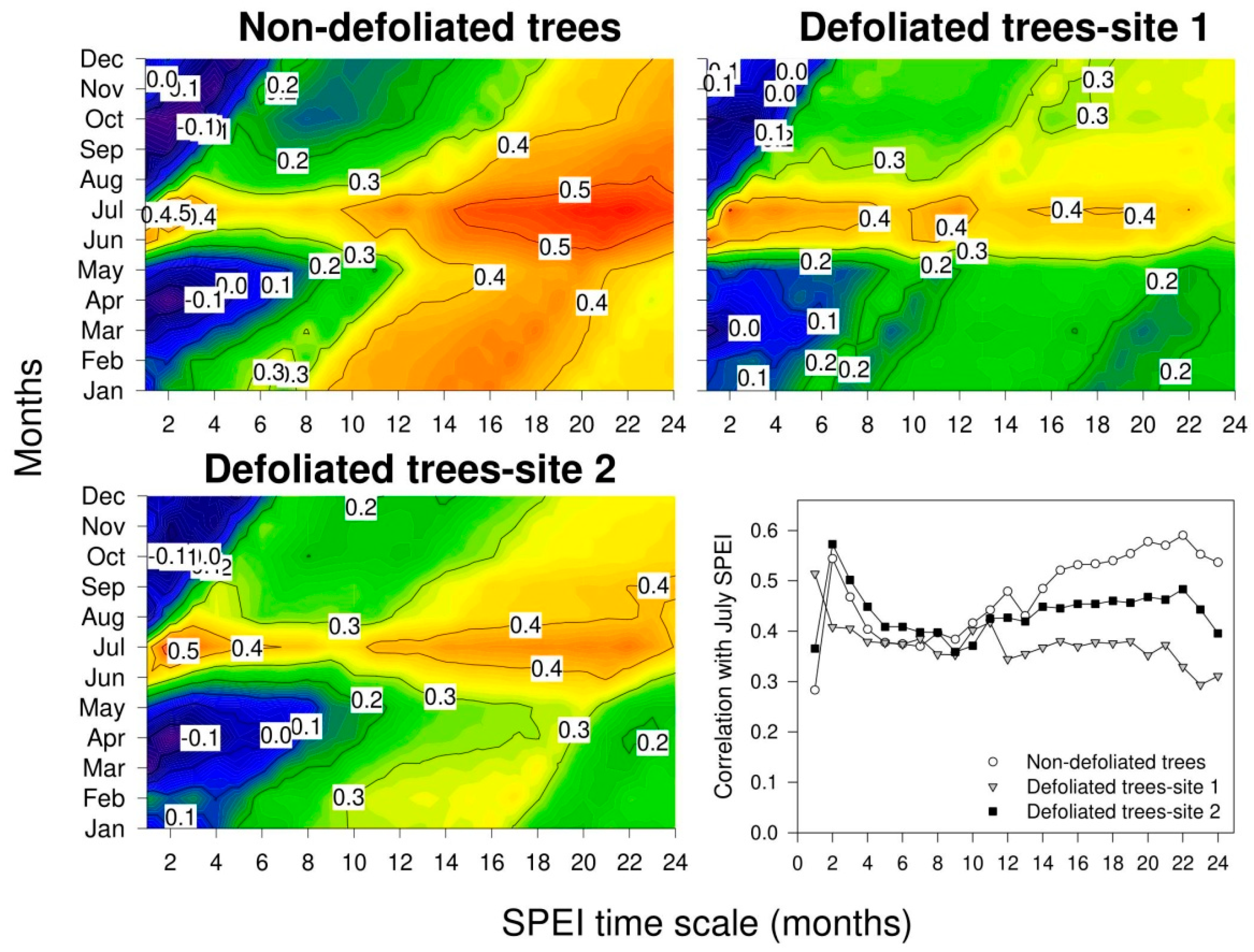
3.4. Growth Responses to Climate Variability

Growth decreased during the years with dry summer conditions such as 2012. A severe growth reduction was observed during that year with relative decreases of −39.4%, −38.1% and −34.2% in the ND, D1 and D2 sites, respectively (Figure 3). On average, tree-ring width decreased from 1.87 to 1.18 mm from 2011 to 2012.
At the site level, growth was enhanced by wet and cool conditions from June to July (Figure 5). The indexed ring-width series of D1 and D2 sites showed a stronger response to June–July temperature and precipitation as compared with the series of the ND site. Specifically, tree growth was more affected by warm and dry summers in the D1 and D2 sites than in the ND site.
The highest correlations between growth rates and the SPEI were observed in June and July at short (2 month) to long (16–22 months) time scales (Figure 6). In the ND and D2 sites, growth responded to drought at short and long time scales, but in the D1 site the strongest responses were observed at short time scales.
At the individual level, correlations between indexed ring-width series with June–July precipitation or temperature did not differ between the two defoliated sites so we analyzed them together (U = 141, p = 0.70 and U = 124, p = 0.35, respectively). We found a higher responsiveness to June–July precipitation in defoliated (mean ± SD correlation = 0.44 ± 0.08) than in non-defoliated (0.37 ± 0.07) trees (U = 77, p = 0.04). In the case of correlations with June–July temperature, no difference was observed between defoliated and non-defoliated trees (U = 278, p = 0.71), but older trees responded more to June–July temperature (Figure S4).

4. Discussion

Using complementary approaches, remote sensing and tree-ring data, we were able to uncover how defoliation caused by outbreaks and drought differently impacted tree cover and radial growth. The two studied disturbances, drought and SSM outbreak, caused radial growth reductions leading to negative shifts in forest productivity. However, only the SSM outbreak was followed by stand defoliation and mortality triggering a negative shift towards reduced tree cover. The growth reduction due to SSM defoliation (−95.7%) was three times higher, in absolute terms, than that caused by the 2012 severe summer drought (−37.2%). The very warm and dry summer conditions during 2012 led to substantial growth decline (a negative growth shift) which agrees with the observed growth responsiveness to the climate of the study Siberian spruce stands. Furthermore, if SSM outbreaks follow similar droughts, huge amounts of dead wood could accumulate and dead or severely defoliated stands could fuel large wildfires across the Siberian taiga as those observed in 2012 [23].
Most boreal spruce forests have showed negative growth trends as the climate warmed, which has been interpreted as a response to temperature-induced drought stress, particularly in the southern Eurasia taiga [48]. Several studies have reported a dominant role of summer water availability to tree growth in the southern and middle taiga [23,49,50,51,52]. Our findings agree with these observations since the growth of the study stands was constrained by warm and dry June to July conditions. Siberian spruce growth was sensitive to short to long summer droughts according to the analyses based on the SPEI, with minor differences between sites. At the individual level, spruce growth was more responsive to changes in June–July precipitation in defoliated than in non-defoliated trees. This difference would suggest a higher growth sensitivity to summer drought in trees from stands prone to SSM defoliation. A major caveat to this finding is the limited number of analyzed sites. Thus, this idea should be tested by comparing more sites, stand structures and tree species in future SSM outbreaks.
Since the NDII negative shift occurred after the SSM outbreak, we can conclude it was probably caused by massive insect defoliation, which is in line with what [12] already reported. Paradoxically, the very warm and dry conditions during summer 2012 reduced wood production but increased tree cover and greenness, according to the NDII, which suggests productivity was potentially enhanced by that drought but the photosynthesized carbon was used in other carbon sinks or functions such as primary growth (bud, shoot, leaf, fine roots), storage or respiration. Remote sensing multispectral data, particularly when combined with tree-ring data, contribute to the ability to better assess the impacts of SSM outbreaks and other stressors such as drought on forest productivity.
A rise in land surface temperature has been observed 2–3 years prior to SSM outbreaks [26]. We also found elevated temperatures and a reduced diurnal thermal range two years before the SSM outbreak in 2016, whilst that year was characterized by warm conditions from late winter to early spring and elevated precipitation in summer followed by a dry early autumn. Overall, these conditions have been seen to favor the development of SSM outbreaks in the taiga zone [2,6,12]. A drop in NDVI from 2018 to 2019 was also reported by [26], which concurs with the negative shift in NDII we found. Therefore, studies based on remote sensing and climate data have a high potential to forecast SSM outbreaks, thus providing early warning signals of pest damage.
Promoting mixed conifer forests dominated by less palatable (e.g., Scots pine; cf. [53]) or non-host species such as birch and managing the understory (e.g., reducing the depth of the moss litter) could help slow down the SSM spread and mitigate the impacts of SSM outbreaks on tree growth [2,54]. Local differences between sites’ conditions, due to the prevalence of SSM outbreaks in gentle sites with deep litter [30], could explain why we found that trees affected by the defoliation responded more to changes in summer water availability before the outbreak started. Alternatively, stands affected by SSM outbreak could have been weakened by a higher drought stress in 2012. Climate warming could promote more severe SSM outbreaks if dry and warm summer conditions become more frequent, but increased temperature variability is also a component of climate warming which would negatively impact on SSM larvae survival through autumn freeze–thaw cycles or more variable and less continental winter conditions. Year-to-year thermal variability could explain why some lepidopteran pests do not always positively respond to climate warming by shifting upwards or polewards as expected (e.g., [16]), whereas many bark beetles do [55]. Increased thermal variability in autumn or winter has been suggested to be a major limiting factor of the westward SSM spread towards Scandinavia [29]. However, warm and dry conditions and a reduced thermal diurnal range could also trigger SSM outbreaks or further contribute to the reduction in tree growth as we observed after the severe 2012 drought. Further studies could also reconstruct the changes in water-use efficiency of taiga forests affected either by drought or by insect outbreaks using H, C and O isotope composition measured in tree-ring wood, xylem and soil water [11,49]. These are retrospective proxies of changes in photosynthesis rate, stomatal conductance and soil water uptake which determine the tree water status, the tree vulnerability to these two stressors and the vitality of trees.

5. Conclusions

To disentangle the long-term impacts on forests of different disturbances or stressors such as drought and insect defoliation, complementary disciplines should be used. By reconstructing changes in tree cover, using remote sensing information (NDII), and radial growth, using dendroecological methods, we were able to reveal how defoliation and massive tree mortality after an insect outbreak reduced canopy cover and growth whereas growing-season drought mainly reduced growth. NDII and growth abruptly declined two years after the SSM outbreak started in 2016 leading to a negative shift in taiga forest productivity, whereas the 2012 summer drought did not reduce NDII. We argue in favor of further research on different disturbances affecting boreal forests to determine their impacts on productivity due to long-term shifts and changes in tree cover and growth. In particular, it should be better investigated if sites where trees show a higher growth responsiveness to growing-season water availability are more predisposed to SSM-outbreak defoliation.

Supplementary Materials

The following are available online at www.mdpi.com/article/10.3390/f13050768/s1, Figure S1: Monthly climate conditions and climate water balance; Figure S2: (a) June–July mean temperature, (b) total precipitation and 2-month July SPEI values in the study area; Figure S3: Monthly climatic anomalies from 2012 to 2017 compared with 1981–2010 averages or totals; Figure S4: Positive relationship found between tree age estimated at 1.3 m and the Pearson correlation obtained by relating individual, indexed ring-width series vs. mean June–July temperatures; Figure S5: Regime shift analyses of spruce tree growth patterns in the three study stands.

Author Contributions

Conceptualization, J.J.C. and T.A.S.; formal analyses, J.J.C. and M.P.; resources, T.A.S. and J.J.C.; data curation, J.J.C. and M.P.; writing—original draft preparation, J.J.C.; writing—review and editing, J.J.C., T.A.S. and M.P.; supervision, J.J.C. All authors have read and agreed to the published version of the manuscript.

Funding

This research was funded by the European Union’s Seventh Framework Programme (INTERACT project), grant agreement BOREALFIRE.

Institutional Review Board Statement

Not applicable.

Informed Consent Statement

Not applicable.

Data Availability Statement

The data presented in this study are available on request from the corresponding author.

Acknowledgments

We thank R.C. Scholten, C.J.F. Delcourt and N.V. Gorina for their help during field sampling.

Conflicts of Interest

The authors declare no conflict of interest. The funders had no role in the design of the study, in the collection, analyses, or interpretation of data, in the writing of the manuscript or in the decision to publish the results.

References

  1. Millar, C.I.; Stephenson, N.L. Temperate forest health in an era of emerging megadisturbance. Science 2015, 349, 823–826. [Google Scholar] [CrossRef] [PubMed]
  2. Rojkov, A.S. Siberian Silk Moth Outbreak and Pest Control; Nauka: Moskow, Russia, 1965. (In Russian) [Google Scholar]
  3. Pureswaran, D.; Grandpré, L.; Paré, D.; Taylor, A.; Barrette, M.; Morin, H.; Régnière, J.; Kneeshaw, D.D. Climate–induced changes in host tree-insect phenology may drive ecological state-shift in boreal forests. Ecology 2015, 96, 1480–1491. [Google Scholar] [CrossRef]
  4. Kharuk, V.I.; Demidko, D.A.; Fedotova, E.V.; Dvinskaya, M.L.; Budnik, U.A. Spatial and temporal dynamics of Siberian silk moth large-scale outbreak in dark-needle coniferous tree stands in Altai. Contemp. Probl. Ecol. 2016, 9, 711–720. [Google Scholar] [CrossRef]
  5. Kolb, T.E.; Fettig, C.J.; Ayres, M.P.; Bentz, B.J.; Hicke, J.A.; Mathiasen, R.; Stewart, J.E.; Weed, A.S. Observed and anticipated impacts of drought on forests insects and diseases in the United States. For. Ecol. Manag. 2016, 380, 321–334. [Google Scholar] [CrossRef]
  6. Kondakov, Y.P. Siberian silk moth outbreaks in Krasnoyarskii krai. In Entomology Researches in Siberia; KF REO: Krasnoyarsk, Russia, 2002; pp. 25–74. (In Russian) [Google Scholar]
  7. Kharuk, V.I.; Im, S.T.; Yagunov, M.N. Migration of the northern boundary of the Siberian silk moth. Contemp. Probl. Ecol. 2018, 11, 26–34. [Google Scholar] [CrossRef]
  8. Kondakov, Y.P. Patterns of Siberian silk moth outbreaks. In Ecology of Forest Animal Populations in Siberia; Nauka: Novosibirsk, Russia, 1974; pp. 206–264. (In Russian) [Google Scholar]
  9. Kharuk, V.I.; Ranson, K.J.; Kuz’michev, V.V. Landsat-based analysis of insect outbreaks in southern Siberia. Can. J. Rem. Sens. 2003, 29, 286–297. [Google Scholar] [CrossRef]
  10. EPPO. Data sheets on quarantine pests: Dendrolimus sibiricus and Dendrolimus superans. EPPO Bull. 2005, 35, 390–395. [Google Scholar] [CrossRef]
  11. Choat, B.; Jansen, S.; Brodribb, T.M.; Cochard, H.; Delzon, S.; Bhaskar, R.; Bucci, S.J.; Field, T.S.; Gleason, S.M.; Hacke, U.G.; et al. Global convergence in the vulnerability of forests to drought. Nature 2012, 491, 752–755. [Google Scholar] [CrossRef] [Green Version]
  12. Kharuk, V.I.; Im, S.T.; Soldatov, V.V. Siberian silkmoth outbreaks surpassed geoclimatic barrier in Siberian Mountains. J. Mt. Sci. 2020, 17, 8. [Google Scholar] [CrossRef]
  13. Serreze, M.C.; Walsh, J.E.I.; Chapin, F.S.; Osterkamp, T.; Dyurgerov, M.; Romanovsky, V.; Oechel, W.C.; Morison, J.; Zhang, T.; Barry, R.G. Observational evidence of recent change in the northern high-latitude environment. Clim. Chang. 2000, 46, 159–207. [Google Scholar] [CrossRef]
  14. Groisman, P.Y.; Blyakharchuk, T.A.; Chernokulsky, A.V.; Arzhanov, M.M.; Marchesini, L.B.; Bogdanova, G.; Borzenkova, I.I.; Bulygina, O.N.; Karpenko, A.A. Climate changes in Siberia. In Regional Environmental Changes in SIBERIA and Their Global Consequences; Groisman, P., Gutman, G., Eds.; Springer: Dordrecht, The Netherlands, 2013; pp. 57–109. [Google Scholar]
  15. Baranchikov, Y.N.; Montgomery, M.E. Siberian Moth: (Dendrolimus sibiricus [Chetverikov]) (Lepidoptera: Lasiocampidae). In The Use of Classical Biological Control to Preserve Forests in North America; United States Department of Agriculture, Forest Service, Forest Health Technology Enterprise Team: Morgantown, WV, USA, 2014; pp. 383–391. [Google Scholar]
  16. Camarero, J.J.; Tardif, T.; Gazol, A.; Conciatori, F. Pine processionary moth outbreaks cause longer growth legacies than drought and are linked to the North Atlantic Oscillation. Sci. Total Environ. 2022, 819, 153041. [Google Scholar] [CrossRef] [PubMed]
  17. Andersen, T.; Cartensen, J.; Hernández-García, E.; Duarte, C.M. Ecological thresholds and regime shifts: Approaches to identification. Trends Ecol. Evol. 2009, 24, 49–57. [Google Scholar] [CrossRef] [PubMed] [Green Version]
  18. Stuart-Haëntjens, E.J.; Curtis, P.S.; Fahey, R.T.; Vogel, C.S.; Gough, C.M. Net primary production of a temperate deciduous forest exhibits a threshold response to increasing disturbance severity. Ecology 2015, 96, 2478–2487. [Google Scholar] [CrossRef] [PubMed]
  19. Townsend, P.A.; Singh, A.; Foster, J.R.; Rehberg, N.J.; Kingdon, C.C.; Eshleman, K.N.; Seagle, S.W. A general Landsat model to predict canopy defoliation in broadleaf deciduous forests. Remote Sens. Environ. 2012, 119, 255–265. [Google Scholar] [CrossRef]
  20. Kharuk, V.I.; Shushpanov, A.S.; Petrov, I.A.; Demidko, D.A.; Im, S.T.; Knorre, A.A. Fir (Abies sibirica Ledeb.) mortality in mountain forests of the eastern Sayan Ridge, Siberia. Contemp. Probl. Ecol. 2019, 12, 299–309. [Google Scholar] [CrossRef]
  21. Bréda, N.; Badeau, V. Forest tree responses to extreme drought and some biotic events: Towards a selection according to hazard tolerance? C. R. Geosci. 2008, 340, 651–662. [Google Scholar] [CrossRef]
  22. Rodionov, S.N. A sequential algorithm for testing climate regime shifts. Geophys. Res. Lett. 2004, 31, 5. [Google Scholar] [CrossRef] [Green Version]
  23. González de Andrés, E.; Shestakova, T.A.; Scholten, R.C.; Delcourt, C.J.F.; Gorina, N.V.; Camarero, J.J. Changes in tree growth synchrony and resilience in Siberian Pinus sylvestris forests are modulated by fire dynamics and ecohydrological conditions. Agric. For. Meteorol. 2022, 312, 108712. [Google Scholar] [CrossRef]
  24. Menne, M.J.; Williams, C.N.; Gleason, B.E.; Jared Rennie, J.; Lawrimore, J.H. The global historical climatology network monthly temperature dataset, version 4. J. Clim. 2018, 31, 9835–9854. [Google Scholar] [CrossRef]
  25. Kovalev, A.; Soukhovolsky, V. Analysis of forest stand resistance to insect attack according to remote sensing data. Forests 2021, 12, 1188. [Google Scholar] [CrossRef]
  26. Kirichenko, N.I.; Baranchikov, Y.N.; Vidal, S. Performance of the potentially invasive Siberian moth Dendrolimus superans sibiricus on coniferous species in Europe. Agric. For. Entomol. 2009, 11, 247–254. [Google Scholar] [CrossRef]
  27. Baranchikov, Y.N.; Tchebakova, N.; Kirichenko, N.; Parphenova, E.; Korezts, M.; Kenis, M. Biological invasions: The Siberian moth, Dendrolimus superans sibiricus, a potential invader in Europe? In Atlas of Biodiversity Risk; Settele, J., Penev, L., Georgiev, T., Grabaum, R., Grobelnik, V., Hammen, V., Klotz, S., Kotarac, M., Kuehn, I., Eds.; Pensoft Publ.: Sofia, Bulgaria, 2010. [Google Scholar]
  28. Flø, D.; Rafoss, T.; Wendell, M.; Sundheim, L. The Siberian moth (Dendrolimus sibiricus), a pest risk assessment for Norway. For. Ecosyst. 2020, 7, 48. [Google Scholar] [CrossRef]
  29. Sultson, S.M.; Goroshko, A.A.; Verkhovets, S.V.; Mikhaylov, P.V.; Ivanov, V.A.; Demidko, D.A.; Kulakov, S.S. Orographic factors as a predictor of the spread of the Siberian silk moth outbreak in the mountainous southern taiga Forests of Siberia. Land 2021, 10, 115. [Google Scholar] [CrossRef]
  30. Kharuk, V.I.; Antamoshkina, O.A. Impact of silkmoth outbreak on taiga wildfires. Contemp. Probl. Ecol. 2017, 10, 556–562. [Google Scholar] [CrossRef]
  31. Dudin, V.A. Use and restoration of silkmoth-damaged forests in Tomsk oblast. Tr. Lesn. Khoz. Sib. 1958, 4, 262–268. [Google Scholar]
  32. Hansen, M.C.; Potapov, P.V.; Moore, R.; Hancher, M.; Turubanova, S.; Tyukavina, A.; Thau, D.; Stehman, S.V.; Goetz, S.J.; Loveland, T.R.; et al. High-resolution global maps of 21st-century forest cover change. Science 2013, 342, 850–853. [Google Scholar] [CrossRef] [Green Version]
  33. Fritts, H.C. Tree-Rings and Climate; Academic Press: London, UK, 1976. [Google Scholar]
  34. Holmes, R.L. Computer-assisted quality control in tree-ring dating and measurement. Tree-Ring Bull. 1983, 43, 69–78. [Google Scholar]
  35. Duncan, R.P. An evaluation of errors in tree age estimates based on increment cores in kahikatea (Dacrycarpus dacrydioides). N. Z. Nat. Sci. 1989, 16, 31–37. [Google Scholar]
  36. Bunn, A.; Korpela, M.; Biondi, F.; Campelo, F.; Mérian, P.; Qeadan, F.; Zang, C. dplR: Dendrochronology Program Library in R; R Package Version 1.7.1; dplR: Milperra, Australia, 2020. [Google Scholar]
  37. R Core Team. R: A Language and Environment for Statistical Computing; R Foundation for Statistical Computing: Vienna, Austria, 2021; Available online: https://www.R-project.org/ (accessed on 11 January 2022).
  38. Briffa, K.R.; Jones, P.D. Basic chronology statistics and assessment. In Methods of Dendrochronology: Applications in the Environmental Sciences; Kluwer Acad. Publ.: Dordrecht, The Netherlands, 1990; pp. 137–152. [Google Scholar]
  39. Vicente-Serrano, S.M.; Beguería, S.; López-Moreno, J.I. A multiscalar drought index sensitive to global warming: The standardized precipitation evapotranspiration index. J. Clim. 2010, 23, 1696–1718. [Google Scholar] [CrossRef] [Green Version]
  40. Beguería, S.; Vicente-Serrano, S.M.; Reig, F.; Latorre, B. Standardized precipitation evapotranspiration index (SPEI) revisited: Parameter fitting, evapotranspiration models, tools, datasets and drought monitoring. Int. J. Climatol. 2014, 34, 3001–3023. [Google Scholar] [CrossRef] [Green Version]
  41. Zang, C.; Biondi, F. Treeclim: An R package for the numerical calibration of proxy-climate relationships. Ecography 2015, 38, 431–436. [Google Scholar] [CrossRef]
  42. Hantson, S.; Chuvieco, E. Evaluation of different topographic correction methods for Landsat imagery. Int. J. Appl. Earth Obs. Geoinf. 2011, 13, 691–700. [Google Scholar] [CrossRef]
  43. Roy, D.P.; Kovalskyy, V.; Zhang, H.K.; Vermote, E.F.; Yan, L.; Kumar, S.S.; Egorov, A. Characterization of Landsat-7 to Landsat-8 reflective wavelength and normalized difference vegetation index continuity. Remote Sens. Environ. 2016, 185, 57–70. [Google Scholar] [CrossRef] [Green Version]
  44. Hardisky, M.; Klemas, V.; Smart, R. The Influences of soil salinity, growth form, and leaf moisture on the spectral reflectance of Spartina alterniflora canopies. Photogramm. Eng. Remote Sens. 1983, 49, 77–83. [Google Scholar]
  45. Rodionov, S.N. A brief overview of the regime shift detection methods. Large-scale disturbances (regime shifts) and recovery in aquatic ecosystems: Challenges for management toward sustainability. In Proceedings of the UNESCO-ROSTE/BAS Workshop on Regime Shifts, Varna, Bulgaria, 14–16 June 2005; pp. 17–24. [Google Scholar]
  46. Rodionov, S.N. Use of prewhitening in climate regime shift detection. Geophys. Res. Lett. 2006, 33, 245. [Google Scholar] [CrossRef] [Green Version]
  47. Stirnimann, L.; Conversi, A.; Marini, S. Detection of regime shifts in the environment: Testing “STARS” using synthetic and observed time series. ICES J. Mar. Sci 2019, 76, 2286–2296. [Google Scholar] [CrossRef]
  48. Lloyd, A.H.; Bunn, A.G. Responses of the circumpolar boreal forest to 20th century climate variability. Environ. Res. Lett. 2007, 2, 045013. [Google Scholar] [CrossRef]
  49. Kagawa, A.; Naito, D.; Sugimoto, A.; Maximov, T.C. Effects of spatial and temporal variability in soil moisture on widths and δ13C values of eastern Siberian tree rings. J. Geophys. Res. 2003, 108, 4500. [Google Scholar] [CrossRef]
  50. Belokopytova, L.V.; Babushkina, E.A.; Zhirnova, D.F. Climatic response of conifer radial growth in forest-steppes of South Siberia: Comparison of three approaches. Contemp. Probl. Ecol. 2018, 11, 366–376. [Google Scholar] [CrossRef] [Green Version]
  51. Shestakova, T.A.; Gutiérrez, E.; Valeriano, C.; Lapshina, E.; Voltas, J. Recent loss of sensitivity to summer temperature constrains tree growth synchrony among boreal Eurasian forests. Agric. For. Meteorol. 2019, 268, 318–330. [Google Scholar] [CrossRef]
  52. Tabakova, M.A.; Arzac, A.; Martínez, E.; Kirdyanov, A.V. Climatic factors controlling Pinus sylvestris radial growth along a transect of increasing continentality in southern Siberia. Dendrochronologia 2020, 62, 125709. [Google Scholar] [CrossRef]
  53. Kirichenko, N.; Flament, J.; Baranchikov, Y.; Gregoire, J.C. Larval performances and life cycle completion of the Siberian moth, Dendrolimus sibiricus (Lepidoptera: Lasiocampidae), on potential host plants in Europe: A laboratory study on potted trees. Eur. J. For. Res. 2011, 130, 1067–1074. [Google Scholar] [CrossRef]
  54. Florov, D.N. Pests of Siberian Forests; OGIX: Irkutsk, Russia, 1948; p. 143. [Google Scholar]
  55. Weed, A.S.; Ayres, M.P.; Hicke, J.A. Consequences of climate change for biotic disturbances in North American forests. Ecol. Monogr. 2013, 83, 441–470. [Google Scholar] [CrossRef]
Figure 1. Location of the study sites in Western Siberia near the Tomsk city (a) and Krasnyi Yar village (b,c) situation of the three study sites. In plot (b) the rectangle indicates the location of the sampled sites near the Krasniy Yar village and Tomsk city. In plot (c) the red patches indicate areas with forest cover loss between 2000 and 2019 based on the analysis of Landsat images according to Global Forest Change data [24].
Forests 13 00768 g001
Figure 2. Monthly climate variables measured in 2016 (triangles), when the SSM outbreak started, as compared with mean values for the period 1950–2020 (excluding the year 2016). Error bars are 95% confidence intervals. The striped area indicates the months with maximum activity of SSM larvae. DTR is the diurnal thermal range.
Forests 13 00768 g002
Figure 3. The horizontal lines show a regime shift in 2018 corresponding to significant (p < 0.01) values of the regime shift index in the two defoliated sites (defoliated site 1, grey symbols and line; defoliated site 2, black symbols and line). Green symbols show NDII values for the non-defoliated site.
Forests 13 00768 g003
Figure 4. Growth patterns in the three study sites from (a) 1900 to 2019 and (b) from 1950 to 2019 with the results of regime shift analyses for the period 1950–2019. In both plots, mean annual values of ring width are presented with SEs. In the lower plot, the different levels of horizontal lines indicate significant (p < 0.01) values of the regime shift index in the three stands (Non-defoliated trees, green symbols and lines; Defoliated tree site 1, grey symbols and lines; Defoliated tree site 2, black symbols and lines).
Forests 13 00768 g004
Figure 5. Climate–growth relationships based on Pearson correlations calculated between mean series of ring-width indices of the three spruce stands and monthly or seasonal climate data (mean temperature, total precipitation). The window of analyses included from the prior to current September with months of the previous year abbreviated by lowercase letters. The last bars correspond to June–July (JJ). The dashed and dotted horizontal lines show the 0.05 and 0.01 significance levels, respectively. Correlations were calculated for the period 1950–2016.
Forests 13 00768 g005
Figure 6. Drought–growth relationships based on the Pearson correlations calculated between mean series of ring-width indices of the three spruce stands and monthly SPEI data. The SPEI was calculated for 1- to 24-month scales (x axes) and from January to December (y axes). The line scatter plot shows the correlation with the July SPEI. Correlation coefficients (r) were calculated for the period 1950–2016 and they were significant at the 0.05 and 0.01 levels for r > 0.22 and r > 0.36, respectively.
Forests 13 00768 g006
Table 1. Sites’ geographical features including latitude, longitude and elevation.
Site (Code)Latitude NLongitude EElevation (m a.s.l.)
Defoliated 1 (D1)57°09′01″84°43′01″137
Defoliated 2 (D2)57°08′12″84°42′01″102
Not defoliated (ND)57°08′33″84°42′25″197
Table 2. Characteristics of sampled trees and tree-ring data. Dendrochronological variables were calculated over the common period 1947–2019.Variables’ abbreviations: AR1, first-order autocorrelation; MSx, mean sensitivity; rbar, mean inter-series correlation. Values are means ± SD.
SiteDBH (cm)No. Trees (No. Cores)Age at 1.3 m (Years)Tree-Ring Width (mm)TimespanAR1MSxrbar
D129.6 ± 10.717 (34)72 ± 221.64 ± 1.051865–20190.46 ± 0.130.29 ± 0.040.41 ± 0.12
D236.3 ± 11.018 (36)79 ± 241.93 ± 1.251876–20190.37 ± 0.170.27 ± 0.030.44 ± 0.14
ND36.7 ± 8.617 (34)77 ± 331.76 ± 1.171876–20190.39 ± 0.160.27 ± 0.040.39 ± 0.18
Publisher’s Note: MDPI stays neutral with regard to jurisdictional claims in published maps and institutional affiliations.

