Using Ground Penetrating Radar (GPR) to Predict Log Moisture Content of Commercially Important Canadian Softwoods

Abstract

The non-destructive testing of wood fibre properties is crucial for informing forest management decisions and achieving optimal resource utilization. Moisture content (MC) is an important indicator of wood freshness and may reveal the presence of wood degradation. However, efficient methods are still needed to better monitor this property along the forest–wood value chain. The objective of the study was to develop prediction models to evaluate log MC based on the propagation of ground penetrating radar (GPR) signals. A total of 165 trees representing four species (black spruce (Picea mariana (Mill.) B.S.P.), white spruce (Picea glauca (Moench) Voss), red spruce (Picea rubens Sarg.), and balsam fir (Abies balsamea (L.) Mill.)) were harvested in two regions of the province of Quebec. GPR signals were acquired in the green (fresh) state and at three subsequent drying stages. Partial least squares regression (PLSR) and locally weighted PLSR (LWPLSR) were employed to establish relationships between GPR signals (antenna frequency: 1.6 GHz) and log properties. The models were fitted on three calibration sets containing four drying stages and different species mixes. The LWPLSR models performed better than the PLSR models for predicting log MC, with a lower root mean square error (RMSEp range: 10.8%–20.2% vs. 13.0%–20.5%) and a higher R²p (0.63–0.87 vs. 0.62–0.82). Spruce-only models performed considerably better than fir-only models while multi-species models were in-between. Despite the complex anisotropy of wood and the physics of wave propagation, the GPR technology can be successfully used to estimate log moisture content, but the GPR-based MC models should be calibrated for each specific type of wood material.

1. Introduction

The Canadian timber supply is currently shrinking due to climate-related disturbances (insects, wildfires) that increase tree mortality [1,2]. Furthermore, salvage harvesting induces more variation in fibre supply because of the complex spatiotemporal dynamics of natural disturbances that affect trees in different ways [3]. This additional variability in turn increases the need for efficient upfront measurements of timber properties and advanced process control to meet product specifications. Adapting harvest and manufacturing processes to timber variability is therefore essential for an optimal and sustainable utilization of wood. In eastern Canada, massive timber volumes have recently been lost due to severe spruce budworm outbreaks. Multiyear defoliation has reduced tree growth and ultimately led to tree death. The cumulative effects of natural disturbances on growth and wood quality are poorly documented. Many questions remain to be answered. How can we monitor potential changes in wood quality from healthy to defoliated and dead trees to better inform salvage operations? Is it worth harvesting and processing dead trees given their internal condition? In this context, moisture content (MC) is an important parameter for evaluating the internal condition of trees and wood logs. MC is also known to be a major driver of biological wood degradation, but its in situ evaluation is complex. The development of non-destructive techniques and tools to monitor wood MC along the forest–wood value chain is greatly needed.

Ground penetrating radar (GPR) has been widely used to evaluate the variation of water content in soils [4] and concrete [5]. The wave propagation of GPRs is governed by the electromagnetic properties of a dielectric material such as wood, which is affected by various material properties such as moisture [6]. In recent years, GPR technology has been used for the early detection of health issues or defects in trees [7,8,9,10,11,12]. The GPR technique has been combined with acoustic tomography for tree decay detection [12,13]. Wen et al. (2016) [13] reported that GPR was effective in detecting cavities, decay, and cracks in tree trunks and that the depth of detection by GPR was influenced by the frequency of the electromagnetic wave used, where higher frequencies achieved shallower depths but higher resolution. A literature review on the use of GPR for the evaluation of wood structures highlights some knowledge gaps related to the ability to distinguish the type of internal feature from the GPR output and the ability to identify internal decay [14].

GPR has been shown to be an effective non-destructive tool for measuring MC in logs [6,15]. Redman et al. (2016) [16] investigated the impact of wood sample shape and size on moisture content measurements using a GPR-based sensor and found that sample size and shape affected the accuracy of the GPR-based sensor. The numerical modelling showed that the curvature of the log and closeness of the log ends (or boundaries) had a significant impact on the GPR signal’s amplitude and travel time, resulting in reduced accuracy in MC measurements [16]. The authors suggested that further research is needed to optimize the GPR-based sensor for the measurement of MC in wood logs.

GPR sensors have also been used on in-service wooden structures to detect internal moisture and fungal decay in Douglas-fir beams [17]. The study showed that the accuracy of GPR was affected by factors such as wood density, moisture content, and beam orientation. GPR was also able to identify decay in regions of a timber bridge that were not visible to the naked eye [18].

The global objective of the study was to develop prediction models to evaluate log moisture content based on the propagation of ground penetrating radar signals. We also evaluated the possibility of predicting sapwood, heartwood, and bark moisture contents using GPR. The specific objectives of the study were:

(1)

To develop prediction models to evaluate log moisture content (MC) of four commercially important softwood species based on high-frequency, high-resolution GPR signals acquired in the green state to approximately 10% MC—this range in MC being typically found along the fibre supply chain, from timber to wood products;

(2)

To evaluate whether GPR signals can predict log diameter and bark thickness;

(3)

To evaluate whether detailed knowledge of wood properties, including sapwood and heartwood MC, contributes to the improvement of MC prediction accuracy for newly harvested logs (i.e., in the green state);

(4)

To test and apply the MC prediction models on other materials (degraded logs, live but partially defoliated trees, and dead trees) to see whether the GPR technology could provide information on internal wood MC and potentially be deployed to inform about wood freshness and/or the shelf-life of trees or logs.

This study shows that our GPR-based MC models can successfully predict the moisture content of logs coming from live/sound trees. On the other hand, the GPR-based MC models could not be directly applied to other materials such as decayed/degraded logs (spruces and balsam fir) and standing balsam fir trees (live and dead). It can be concluded that GPR-based MC models should be calibrated for each type of material.

2. Materials and Methods

2.1. Trees

A total of 165 trees were harvested from two sites (

Table 1. Descriptive statistics of black (BS), white (WS), and red (RS) spruce, and balsam (BF) trees harvested from the SOPFIM and Valcartier Forest Research Station (VFRS) sites and selected for ground penetrating radar (GPR) scans. Figures in parentheses are standard deviations. DBH: diameter at breast height; BH: breast height.

Site	Species	No. of Trees	DBH (cm)	Tree Height (m)	Crown Base Height (m)	Cambial Age (BH)
SOPFIM 1	BS	23	15.4 (4.47)	9.9 (2.38)	-	50.8 (16.71)
	WS	23	17.5 (6.07)	10.8 (2.47)	-	49.1 (11.92)
	BF	25	15.4 (3.98)	11.8 (2.81)	-	49.8 (17.27)
CFS 2	BS	15	23.1 (5.41)	18.3 (2.18)	10.1 (1.50)	68.3 (24.93)
	WS	32	22.0 (4.68)	16.0 (3.12)	8.0 (2.91)	51.5 (19.14)
	RS	15	23.6 (6.78)	17.6 (3.38)	11.0 (3.35)	64.2 (16.96)
	BF	32	22.9 (5.51)	16.0 (3.52)	6.5 (3.20)	40.7 (14.24)
Total		165				51.4 (18.71)

¹ One log per tree; ² Two logs per tree.

). The first site was located in the boreal forest of the North Shore region of Québec (e.g., Baie-Comeau/Forestville). This region is periodically affected by spruce budworm (Choristoneura fumiferana) epidemics [3]. The latest outbreak started in 2006, whereas the previous one took place in the 1970s. In late October 2020, 6 representative blocks were selected within an experimental site established by the Société de protection des forêts contre les insectes et les maladies (SOPFIM) (Society for the Protection of Forests against Insects and Diseases). The blocks had received some aerial pesticide spray treatments by the SOPFIM to limit tree defoliation and mortality (i.e., to keep trees alive until the end of the outbreak). Seventy-one trees of merchantable diameter (diameter at breast height (DBH) of 9.1 cm and larger) were harvested within three age classes (30, 50, and 70 years old). The selected trees represented three species: black spruce (Picea mariana (Mill.) B.S.P.) (BS), white spruce (Picea glauca (Moench) Voss) (WS), and balsam fir (Abies balsamea (L.) Mill.) (BF). Sampled trees appeared generally sound (live), but some sample logs had some wood discoloration. One ca. 30-cm long log was cut at breast height from each tree, sealed in a plastic bag and stored in a freezer until analysis.

The second site was located at the Valcartier Research Forest Station managed by the Canadian Forest Service (thereafter called ‘CFS’ site) near Québec City, Canada. This forest region has not been affected by recent spruce budworm outbreaks. A total of 94 healthy trees were randomly selected in three diameter classes—small (12–20 cm), median (20–26 cm), and large (26–32 cm)—in late November through mid-December of 2020. The selected trees consisted of black spruce, white spruce, red spruce (Picea rubens Sarg.) (RS), and balsam fir. To cover within-tree variation in wood properties, sampling was expanded so that two ca. 50-cm long logs were collected from each tree, one at breast height, the other at varying heights above the breast height but within the first 5 m of the trunk to avoid whorls, large knots, and other defects. Logs were also sealed in a plastic bag and kept frozen until processing.

2.2. Determining Wood Properties and Log Moisture Content

Before processing, each log was thawed at room temperature for a few days (inside the plastic bag) to ensure temperature equilibrium with the room (ca. 20 °C). Two ca. 4-cm-thick discs were then extracted from the large end of each log (again avoiding major defects). One of the discs was used for evaluating bark thickness, moisture content (MC) of the bark (MCb), sapwood (MCsw), and heartwood (MChw). Bark thickness was computed as the average of two measurements taken from two positions on the long- and short-diameter axes. The disc was debarked, and the bark weighted. After this step, two small wood blocks (ca. 3 cm × 3 cm) were sawn from two opposite radii (i.e., along one diameter) in the sapwood (close to the bark) and in the heartwood (close to the pith but avoiding it). The two MC values per wood type were then averaged. Each portion was weighed on a scale before and after oven-drying to obtain their initial and oven-dry weight. Wood MC was determined gravimetrically by dividing the difference between the initial and oven-dry weights by the oven-dry weight (i.e., dry basis MC) following the ASTM4442 standard [19]. The other disc was used for measuring cambial age and wood density. Green and basic wood density were determined by the ratio of weight (green and oven-dry, respectively) to green volume using the water immersion method following the ASTM D2395 standard [20]. Average growth ring width was derived from the log diameter and its cambial age.

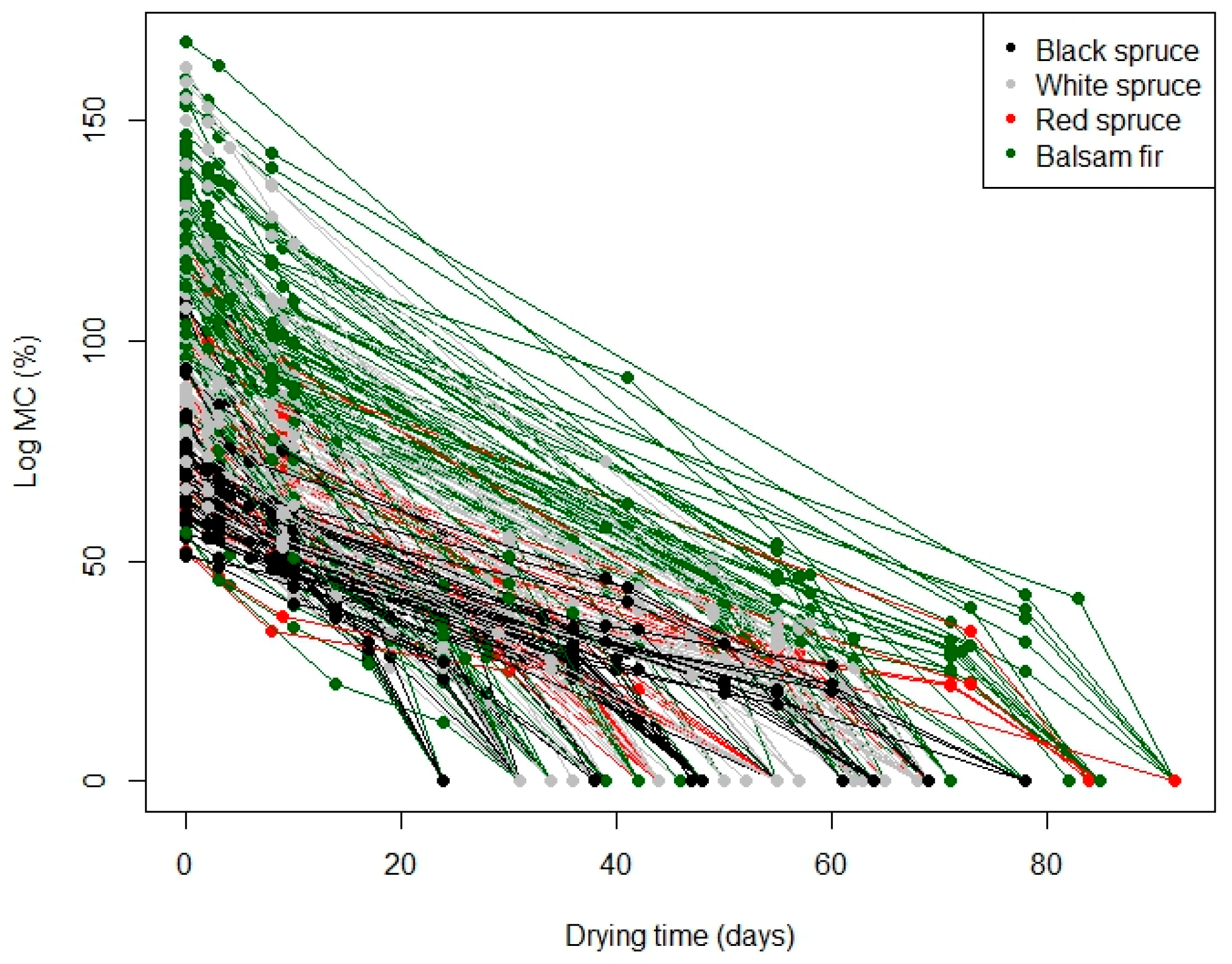
The remaining portion of each log was used for obtaining ground penetrating radar (GPR) signals at different MC levels. Each log was weighed immediately after disc removal and kept at room temperature to air dry. The logs were weighted three more times at variable intervals leading to four different drying stages (Figure 1). The logs were then oven-dried to obtain dry mass. MC for each log at each drying stage was back-calculated from the oven dry weight.

2.3. GPR Signal Acquisition

GPR signals were acquired on 257 logs using a MALÅ CX GPR system (MALÅ Geoscience AB, Malå, Sweden) with a central frequency of 1.6 GHz and an antenna separation of 0.06 m. Scans were acquired during a time window of 8.34 nanoseconds (ns) (containing 312 time-sampling points) at a time interval of 0.01 s. Immediately after weighing, each log was placed on a workbench with an adjustable opening such that there was an empty space underneath the log. GPR signals were recorded with the electromagnetic (EM) field oriented perpendicular to fibre direction and the EM wave propagating along the radial direction [15]. Through-the-bark GPR scans were performed on four positions 90 degrees apart around the middle of the log (Figure 2).

2.4. GPR Signal Processing

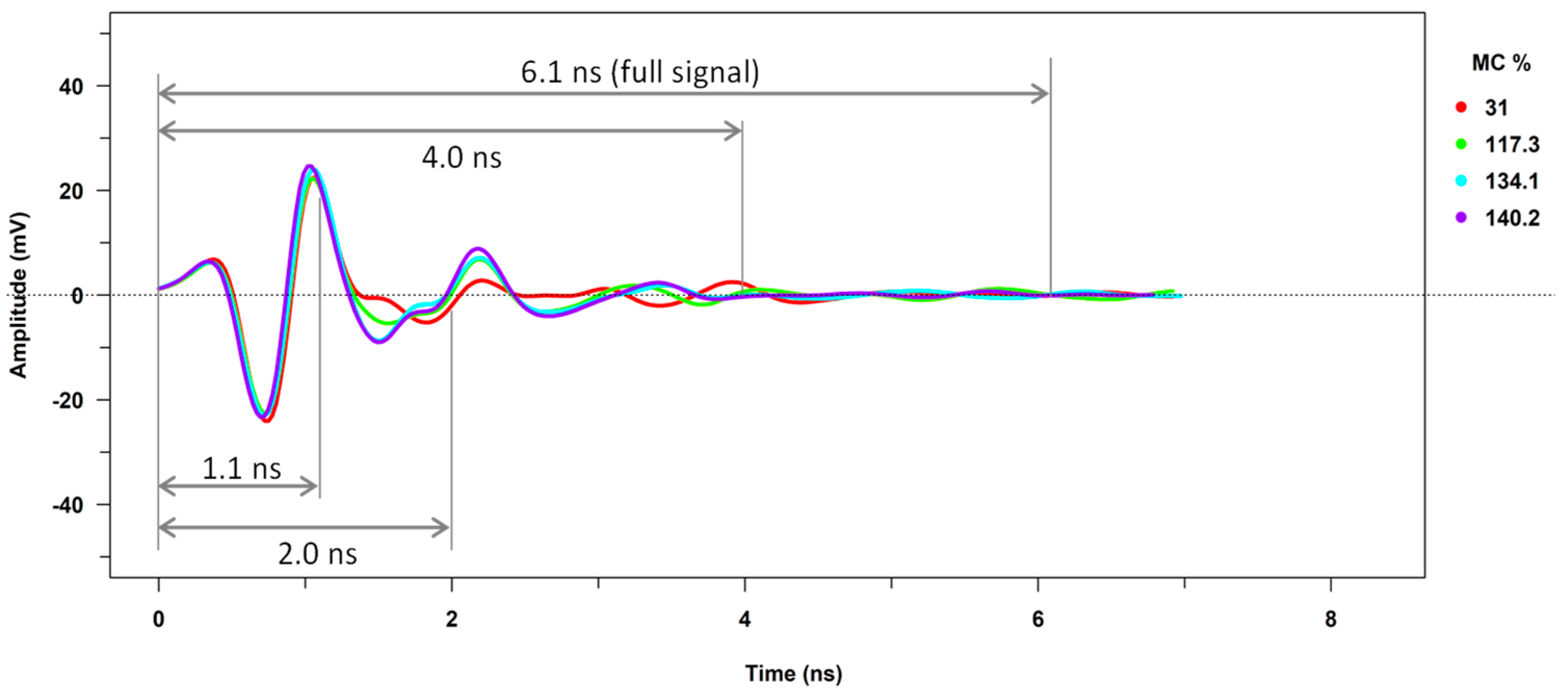
The majority (95%) of the GPR scans produced around 500 traces depending on the duration of each individual scan. Direct current (DC) shift was removed from each trace by subtracting the average of the first 25 amplitude values from each data point in the trace. The arrival time of the direct wavelet of each trace was selected based on a 14% maximum amplitude threshold value [15]. Time zero correction was then applied to each trace according to the selected arrival times so that the traces had the consistent pulse onset times. After pre-processing, the traces contained 228 time-sampling points, which was equivalent to a 6.1 ns signal time window. This signal will be referred to as the full trace/signal hereafter (Figure 3). All traces within each scan were averaged, resulting in a total of 3810 averaged traces (one average trace representing a scan in this case). The four traces from the four scanning positions were further averaged for each log at each drying stage, resulting in 953 traces in total (

Table 2. Moisture content (MC) and number of GPR traces from all logs and four drying stages from each site and species used for modelling. Standard deviations are in parentheses.

Site	Species	No. of Logs	No. of GPR Traces	Log MC (%) Min–Max	Mean Log MC (%)
SOPFIM	BS	23	92	18.1–116.6	56 (23.3)
	WS	23	91	13.4–133.3	65 (30.6)
	BF	25	99	27.4–161.8	74 (33.8)
CFS	BS	30	107	14.1–92.5	50 (17.7)
	WS	64	231	17.6–158.8	75 (33.2)
	RS	30	114	9.1–121.2	64 (26.3)
	BF	62	219	22.6–167.6	92 (39.1)
Total		257	953

). These traces served as the base GPR signal matrix for estimating log MCs from the GPR signals (with observations as rows and time samples as columns). Signal preprocessing was carried out using the RGPR package of the R statistical computing software [21]. Figure 3 presents an example of pre-processed GPR signals collected at four MC levels from the same log.

2.5. Statistical Analysis and Modelling

ANOVA and Pearson correlation coefficients were used to compare log characteristics and wood properties between different sites and species. Partial least squares regression (PLSR) and locally weighted PLSR (LWPLSR) were the models employed to establish relationships between GPR signal matrix and log properties.

PLSR searches for a set of components or latent variables (LVs) that perform a simultaneous decomposition of X (the matrix of GPR signals) and Y (the matrix of target properties) with the constraint that these LVs explain as much of the covariance between X and Y as possible. This is followed by a regression step, where the decomposition of X is used to predict Y. This technique is especially well suited for handling predictors with high-level collinearity as is the case between time samples of GPR signals. Typically, when using PLS regression, a calibration model is built, and its accuracy and robustness are then assessed with an independent validation dataset.

LWPLSR is a particular case of weighted PLSR, with the weights depending on the dissimilarity (e.g., Euclidian or Mahalanobis distances) between calibration observations and new observations to predict [22]. LWPLSR is particularly suited when there are nonlinear relationships between responses and predictors due to the heterogeneity of data [22].

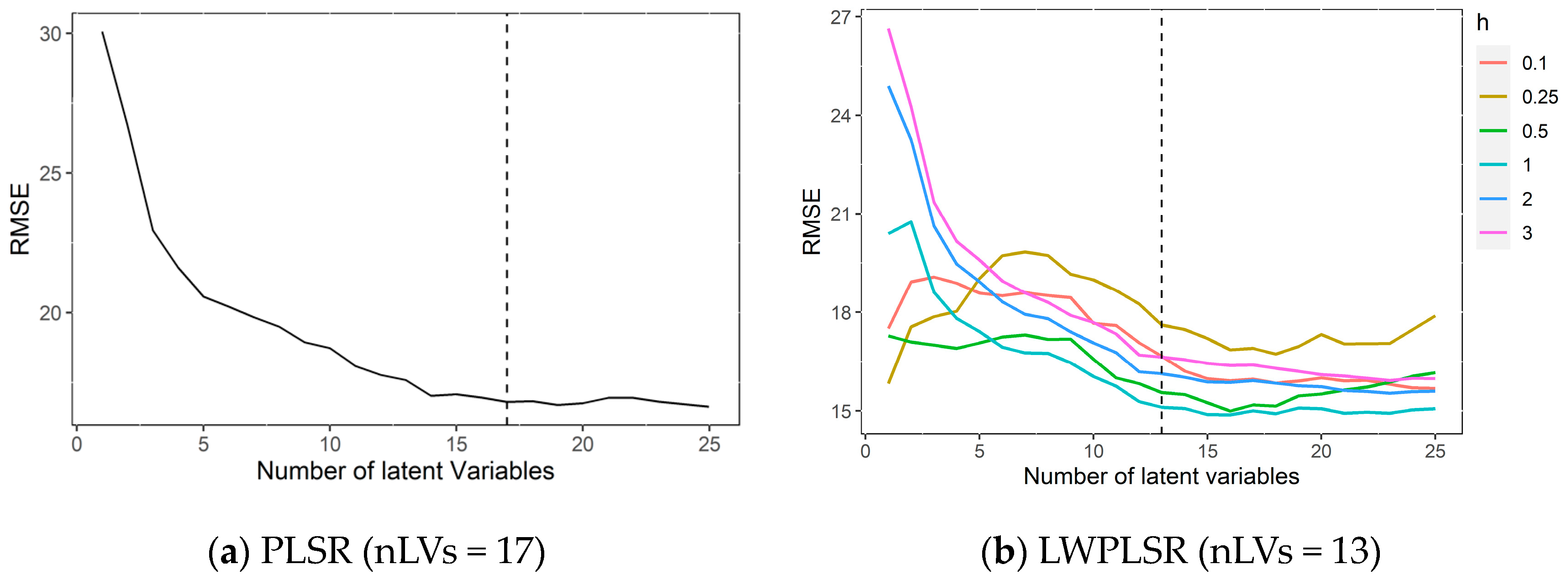
In this paper, both PLSR and LWPLSR models were fitted on the same datasets. The hyper-parameters of the models were tuned with a five-fold cross-validation. The goal of this tuning for the PLSR models was to find the optimal number of latent variables (nLVs) (Figure 4a). For the LWPLSR models, two hyper-parameters were tuned: nLVs and the shape of the weight function, h (Figure 4b). A lower h value implies a sharper weight function [22]. The optimal hyper-parameters were selected based on a single criterion of having the lowest nLVs while RMSE is not greater than the sum of the lowest RMSE and an allowance. The allowance was set at 0.25 for models predicting MCs and 0.0125 for models predicting log diameter and bark thickness. Figure 4 illustrates this process in the case of the log MC model based on the four drying stages and four mixed species.

2.6. Response Variables, Covariate Variables, and Time Window Selection

PLSR and LWPLSR analyses were used to predict log MC from GPR signals (

Table 3. Modelling scheme showing the combinations of parameters in each subset of data for predicting response variables. MC: log moisture content; DOB: log diameter outside bark; THb: bark thickness; MCb: bark moisture content; MCsw: sapwood moisture content; MChw: heartwood moisture content; Db: basic wood density; BF: balsam fir.

Model Group	Response *	Covariate	Species	Drying Stage	Time Window (Sampling Points)	Calibration Size	Validation Size
1	MC	-	Spruces, BF		6.1 ns (228) 4.0 ns (150) 2.0 ns (75) 1.1 ns (40)	654–660	286
		-	Spruces only	1, 2, 3, 4		435–443	191
		-	BF only			218–222	96
2	DOB	-
	THb	-	Spruces, BF	1		164–167	72
3	MC	DOB	Spruces, BF	1, 2, 3, 4
		Thb
		DOB, THb				164–167	72
4	MC	-	Spruces, BF	1		164–167	72
	MCb + MCsw + MChw	-	Spruces, BF	1		164–167	72

* Note: Models for response variables MCb + MCsw + MChw used multivariate approach.

). We also tested whether a universal model for all species had a sufficient prediction accuracy by fitting the models for BF and spruces separately, in addition to all species combined (spruces and BF, multi-). In this case, data from all four drying stages were used (model group 1).

Models were also created to estimate log diameter and bark thickness from GPR signals (model group 3) since previous studies suggested that log diameter is highly correlated to GPR signals [23].

To investigate whether including log diameter and bark thickness as additional predictors (i.e., covariates) increases prediction accuracy, the multi-species models were fitted for GPR signals alone and together with these additional parameters. Since these parameters changed little throughout the drying process, only the data from the 1st drying stage was included in these cases (model group 2).

In addition, attempts were made to predict MCb, MCsw, and MChw from the GPR signals (model group 4) using a multivariate approach, i.e., the PLS-2 regression model (where multiple response variables in the same model are predicted simultaneously). The optimal nLVs of the multivariate model were determined based on the minimum sum of the RMSE for each response variable. Since these five response variables were measured at the first drying stages, only GPR signals from the first drying stage were used.

Each dataset (the combination of response variable(s), time window, species, and drying stage) was split into calibration and validation sets at a ratio of 0.7:0.3. A random seeding was adopted for splitting to ensure a consistent splitting result for reproducibility and comparability of the models. Traces with a Mahalanobis distance falling outside of 3 standard deviations of the mean were removed from each calibration set.

Each time sample in the selected time window was introduced as a predictor in the PLSR and LWPLSR analyses. In general, PLS algorithms automatically centre data (having a mean of zero). For the models that included additional predictors (model group 2), all the predictive variables were further rescaled to have a standard deviation of 1.0 for the calibration set and the same scaling parameters were applied to the validation set. All analyses were performed using the R statistical computing software (v4.03; R Core Team 2020). The rchemo package (v0.0-17; [24]) was employed for tuning the hyper-parameters and fitting the PLSR and LWPLSR models.

3. Results

3.1. Log Characteristics, Wood Properties and MC

As shown in

Table 4. Log characteristics and wood properties of black (BS), white (WS), and red (RS) spruces and balsam fir (BF) from the SOPFIM and CFS Valcartier Forestry Research Station sites for ground penetrating radar (GPR) scans. Numbers in parentheses are standard deviations.

Site	Species	No. of Logs	Log Diameter (cm)	Ring Width (mm)	Basic Density (kg/m3)	Green Wood
						Green Density (kg/m3)	Green Log MC (%)	Sapwood MC (%)	Heartwood MC (%)	Bark MC (%)	Bark Thickness (mm)
SOPFIM	BS	23	16.6 (4.01)	1.9 (0.42)	415 (39.4)	844 (117.6)	79 (15.9)	102 (23.0)	45 (14.7)	109 (26.3)	5.0 (1.05)
	WS	23	19.0 (5.89)	1.9 (0.56)	376 (29.1)	853 (79.7)	94 (21.3)	133 (37.2)	46 (14.2)	120 (32.0)	5.2 (1.63)
	BF	25	17.9 (4.42)	1.9 (0.42)	349 (28.0)	864 (96.7)	107 (23.1)	130 (33.9)	78 (37.9)	108 (18.9)	5.1 (1.35)
CFS	BS	30	21.0 (4.93)	1.8 (0.38)	394 (23.1)	806 (323.6)	65 (9.1)	96 (19.9)	41 (10.5)	92 (24.2)	5.1 (1.47)
	WS	64	19.6 (4.74)	2.4 (1.02)	375 (58.5)	843 (114.8)	99 (22.6)	131 (31.7)	47 (21.8)	112 (18.0)	5.1 (1.20)
	RS	30	21.1 (5.96)	1.9 (0.46)	371 (20.2)	795 (176.1)	83 (17.5)	112 (41.7)	37 (9.7)	100 (13.8)	5.5 (1.29)
	BF	62	20.5 (4.86)	3.1 (1.19)	328 (26.3)	867 (88.1)	123 (16.1)	138 (28.5)	120 (36.8)	93 (14.4)	5.4 (1.37)
Total		257

, the studied logs had similar diameters across all species from the same site. The logs from the SOPFIM site were on average 2.7 cm smaller (p = 0.0003) and had a basic density 13 kg/m³ higher (p = 0.0014) than those from the CFS site. Basic wood density was higher (p = 0.0014) at the SOPFIM site than at the CFS site and followed an expected trend among these species, i.e., BS (high density) > WS > RS > BF (low density). There were little differences in bark thickness among sites or species.

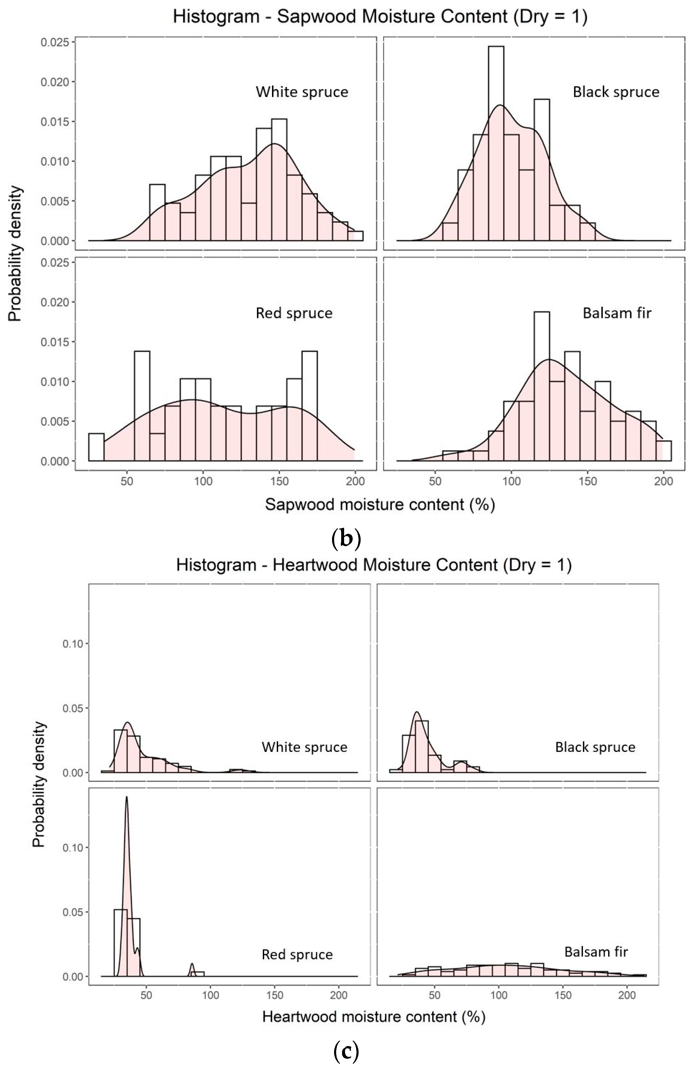
At the green state, BF logs had higher sapwood and heartwood MCs (p = 0.000~0.0013) than spruces. It was also noticed that BS and RS had higher sapwood MCs than WS (p = 0.000~0.013).

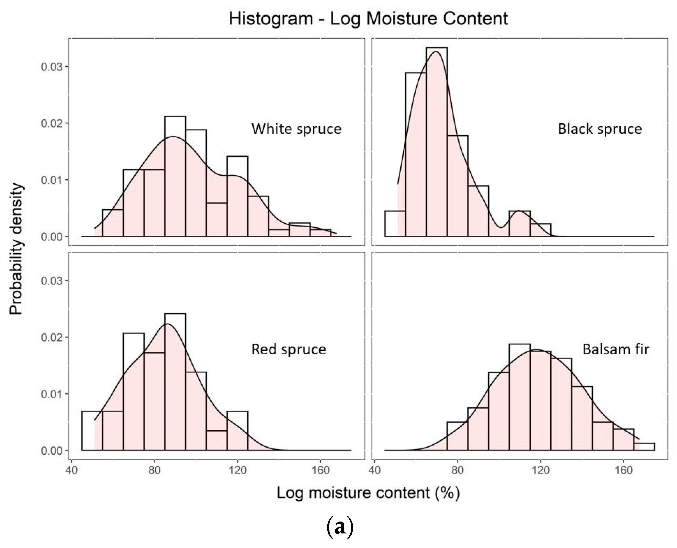
As expected, average log MC had a relatively strong positive correlation with the MC of sapwood (r = 0.72) and heartwood (r = 0.71), and the correlation between average log MC and heartwood MC was less strong in the spruces (r = 0.52) than in BF (r = 0.65). BF heartwood MC (40%–220%) varied over a wider range than average log MC (80%–150%), which may be attributed to the presence of moisture pockets (wetwood) in BF heartwood.

3.2. Comparison of Single and Multi-Species Models

For almost all subsets of the data, the LWPLSR models for predicting log MC had a lower RMSE (10.8%–20.2% vs. 13.0%–20.5%), a higher R²p (0.63–0.87 vs. 0.62–0.82), and a higher RPD (1.7–2.8 vs. 1.6–2.3) than their counterpart PLSR models using the same dataset (

Table 5. Optimum number of latent variables (nLVs), validation coefficients of determination (R²), root mean square errors (RMSE) and ratios of performance to deviation (RPD) from partial least squares regression (PLSR) and locally weighted partial least squares regression (LWPLSR) models predicting log MC from GPR signals of different time window (TW) lengths, ns or number of time-samples (nTS). The models were fitted on three calibration sets containing four drying stages and different species mixes.

Species Mix	nTS (TW)	Calibration n	PLSR				LWPLSR
			nLVs	RMSE	R2	RPD	nLVs	RMSE	R2	RPD
			Validation n = 286
Spruces,	228 (6.1)	660	20	15.80	0.78	2.16	13	13.87	0.83	2.46
Balsam fir	150 (4.0)	655	17	16.37	0.77	2.08	13	14.14	0.83	2.41
	75 (2.0)	654	15	16.93	0.75	2.01	11	15.19	0.80	2.24
	40 (1.1)	659	17	19.80	0.66	1.72	10	19.14	0.68	1.78
			Validation n = 191
Spruces	228 (6.1)	443	20	13.00	0.82	2.34	19	10.82	0.87	2.81
	150 (4.0)	439	16	13.56	0.80	2.24	11	11.67	0.85	2.60
	75 (2.0)	435	14	14.13	0.78	2.15	6	12.60	0.83	2.41
	40 (1.1)	438	15	17.43	0.67	1.74	11	17.95	0.65	1.69
			Validation n = 96
Balsam fir	228 (6.1)	221	12	16.98	0.74	1.97	5	16.26	0.76	2.06
	150 (4.0)	222	12	16.84	0.75	1.99	11	17.07	0.74	1.96
	75 (2.0)	219	17	16.83	0.75	1.99	17	15.72	0.78	2.13
	40 (1.1)	218	14	20.51	0.62	1.63	15	20.21	0.63	1.66

). The optimum number of latent variables was also lower for LWPLSR than for PLSR, which translates to an increase in model robustness. The highest R², lowest RMSE and highest RPD were generally achieved using the GPR signals of 228 time-samples for both models with the exception of BF-only models which exhibited a mixed trend. It is clear that the GPR signals within the early time window of 1.1 ns did not contain enough information about MC in logs.

For both model types, spruce-only models performed considerably better than BF-only ones and multi-species models were in-between.

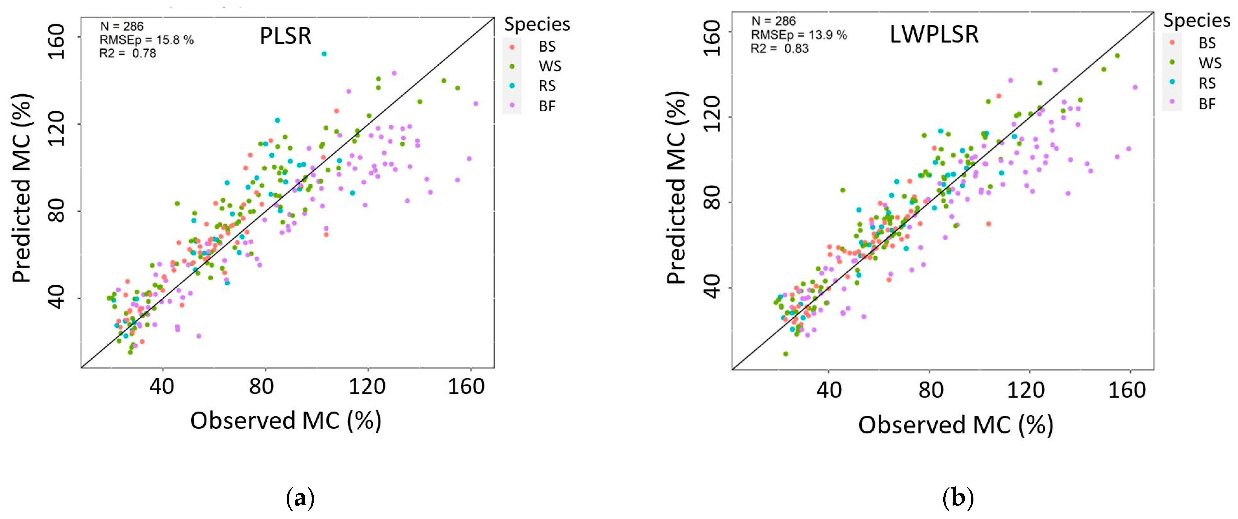
Figure 5 shows that both PLSR and LWPLSR calibrated with all species underestimated BF log MCs and overestimated spruce log MCs. This holds true for the GPR signals of all four time windows (6.1, 4.0, 2.0, and 1.1 ns). In addition, the prediction error appeared to be larger when log MC was higher than 80%, especially for BF (Table 5). This warrants separate models for spruces and BF, as evidenced by the points that were evenly dispersed along the unity lines, with a few exceptions for spruces (Figure 6). Both PLSR and LWPLSR models underestimated WS log MCs when it was higher than 120% (Figure 6).

3.3. Prediction of Log Diameter and Bark Thickness

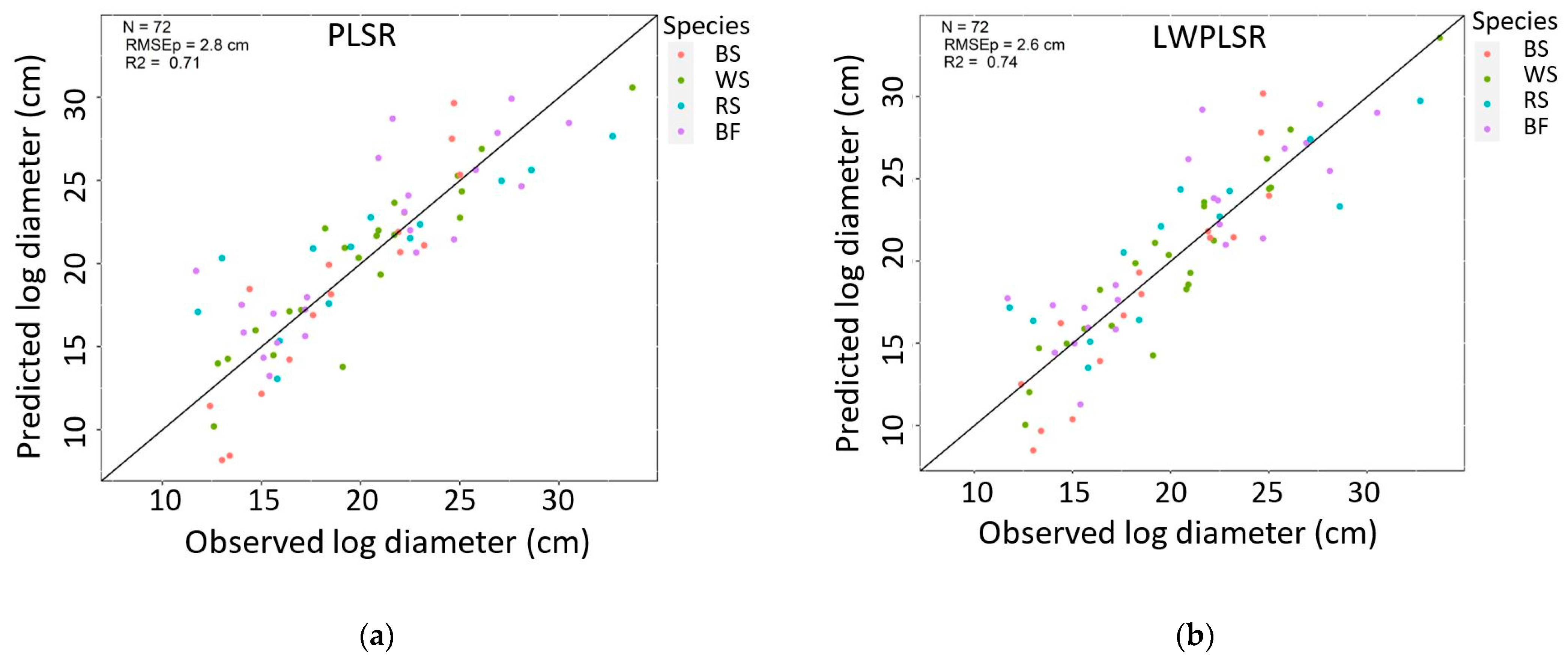
The PLSR and LWPLSR models using full GPR signals presented much better performances for log diameter than for bark thickness prediction (

Table 6. Optimum number of latent variables (nLVs), validation coefficients of determination (R²), root mean square errors (RMSE) and ratios of performance to deviation (RPD) from locally weighted partial least squares regression (LWPLSR) models predicting log diameter and bark thickness from GPR signals. Only the time window (TW) in ns or number of time-samples (nTS) that gave the best overall results are shown. The models were fitted on four calibration sets containing the 1st drying stage for all species. Values shown were results from tests on a validation set of n = 72.

Response Variable	nTS (TW)	Calibration (n)	nLVs	RMSE	R2	RPD
Log diameter	150 (4.0)	167	5	2.26	0.81	2.30
Bark thickness	40 (1.1)	165	3	1.08	0.46	1.37
Log diameter 1	150 (4.0)	167	5	2.31	0.80	2.25
Bark thickness 1	40 (1.1)	165	9	1.11	0.43	1.34

¹ PLS-2 results.

). The LWPLSR model using the 4.0 ns time window accounted for a higher variance (81%) in log diameter with an RPD value of 2.30. In contrast, the PLSR and LWPLSR models were most accurate at predicting bark thickness from GPR signals of 2.0 ns and 1.1 ns, respectively, with approximately 44%–46% variance explained and a prediction error of 1.1–1.2 mm (Figure 7).

3.4. Log Characteristics and Wood Properties as Additional Predictors

PLSR models fitted on the GPR signals from the first drying stage alone had a very poor prediction quality for log MC. For example, when using all species, R² values ranged from 0.02 to 0.31 and RPD from 1.01 to 1.21, depending on the time window. LWPLSR models had similar results.

Table 7. Optimum number of latent variables (nLVs), coefficients of determination (R²), root mean square errors (RMSE) and ratios of performance to deviation (RPD) from locally weighted partial least squares regression (LWPLSR) models predicting log moisture content (MC) from ground penetrating radar (GPR) signals. Only the time window (TW) in ns or number of time-samples (nTS) that gave the best overall results are shown for different sets of additional predictors, including log diameter (DOB), bark thickness (THb), basic wood density (Db), ring width (Wr), and green density (Dg). The models were fitted on a calibration set containing the 1st drying stage and all species (spruces and BF). Values shown were results from tests on a validation set of n = 72. Models by species for all drying stages are shown in Appendix A (Table A1).

Predictors	nTS (TW)	Calibration (n)	nLVs	RMSE	R2	RPD
GPR	150 (4.0)	167	5	20.20	0.33	1.23
GPR, DOB, THb	228 (6.1)	164	12	20.93	0.29	1.19
GPR, DOB, Db	228 (6.1)	164	8	16.78	0.54	1.49
GPR, DOB, Db, THb, Wr, Dg	228 (6.1)	164	14	13.95	0.68	1.79

presents only the best models. Including log diameter and bark thickness as additional predictors of MC did not increase the predictive power of the models when all species were considered (Table 7). However, including log diameter and basic density improved the prediction quality, with an increase in R² values of up to 0.24 for PLSR and up to 0.27 for LWPLSR and decreases in RMSE of up to 3.3% for PLSR and up to 3.9% for LWPLSR. Also, including bark thickness, ring width, and green density further increased R² values by up to 0.31 (PLSR) and 0.46 (LWPLSR). The inclusion of log diameter and basic wood density increased R² values by up to 0.47 (PLSR) and 0.42 (LWPLSR) when only BF was considered, whereas increases were up to 0.30 and 0.40 when including the other three parameters. The RPD values were higher than 1.5 only when all five additional parameters were included in the models (except for models for spruces only).

In general, models for spruces only did not perform well, with R² values swinging from −0.91 to 0.81, depending on the model, species mix and time window. Models for BF only showed the most performance gains by including additional predictors.

3.5. Prediction of Bark, Sapwood and Heartwood MC

The best PLSR model had an R² value of 0.28 for the prediction of bark MC when all species were considered, with an RPD of 1.18 and a time window of 2.0 ns (

Table 8. Optimal number of latent variables (nLVs), coefficients of determination (R²), root mean square errors (RMSE), and ratios of performance to deviation (RPD) from partial least squares regression (PLSR) and locally weighted partial least squares regression (LWPLSR) models predicting bark, sapwood, and heartwood moisture content (MC) from ground penetrating radar (GPR) signals of different time window lengths (TW) in ns or number of time-samples (nTS). The models were fitted on a calibration set containing the 1st drying stage and all species (spruces and BF). Values shown were results from tests on a validation set of n = 72.

Response Variable	Model Type	nTS (TW)	Calibration (n)	nLVs	RMSE	R2	RPD
Bark MC	PLSR	75 (2.0)	166	7	18.16	0.28	1.18
	LWPLSR	40 (1.1)	165	9	18.37	0.26	1.17
Sapwood MC	LWPLSR	150 (4.0)	167	2	28.27	0.30	1.21
Heartwood MC	LWPLSR	150 (4.0)	167	2	27.56	0.21	1.14

). The second-best model was the LWPLSR model with an R² of 0.26. LWPSLR models performed poorly in general, as did the PLSR and LWPLSR models for spruces or BF, many of which had negative R² values. Similarly, most of the models for the prediction of heartwood MC of all species or BF-only had a negative R² value and a high RMSE. Models for spruce heartwood MC had R² values of 0.20–0.41, with the best model being the one using a 1.1 ns time window.

The LWPLSR model using the 4.0 ns time window had the highest R² value (0.30) in predicting sapwood MC when all species were considered (Table 8). When only BF was considered, the prediction accuracy of both PLSR and LWPLSR models increased, with the best model having R² values of 0.34 (time window of 0.4 ns or 0.11 ns) and 0.43 (time window of 2.0 ns), respectively. However, the models for spruces were not stable.

4. Discussion

4.1. Log Characteristics, Wood Properties and MCs

Balsam fir had a markedly higher wood moisture content compared to the other spruces (Table 2); many logs had a very high MC in the heartwood. It is known that the MC of BF heartwood tends to be higher than that of spruces [25]. It is also possible that some trees had not yet developed a distinct heartwood, which is usually characterized by a lower MC compared to sapwood. Finally, the presence of wet pockets that are commonly found in fir species may have influenced the radar signals (i.e., increased variation). Wet pockets have been associated with bacterial infections in live trees. These infections make lumber products more difficult to kiln dry [26,27]. While the three spruces had very similar wood characteristics, balsam fir clearly differed in its moisture content distribution, which influenced the GPR signal differently compared with spruces. The observed differences cannot be attributed to a seasonal variation in MC since all sample trees were harvested in the fall of 2020.

For balsam fir, we could not observe any clear ‘site’ differences in moisture content predictions that could have been linked to the fact that some SOPFIM trees from the North Shore region had been impacted/defoliated by the spruce budworm outbreak over several years (Appendix A, Figure A2).

4.2. Comparison of Single and Multi-Species Models

Partial least squares regression (PLSR) and locally weighted PLSR (LWPLSR) were employed to establish relationships between GPR signals (antenna frequency: 1.6 GHz) and log moisture content. Overall, the LWPLSR models performed better than the PLSR models for predicting log MC.

Spruce-only models performed considerably better than fir-only models, while multi-species models were in-between. We observed that balsam fir behaved differently most likely because the species has a different wood moisture distribution than spruces, and because the species is prone to the development of moisture pockets. The three spruce species considered in this study showed limited variations in annual growth rates, had relatively comparable MC distributions, and shared the same wood anatomical structure. Therefore, it was acceptable to develop ‘genus-specific’ GPR-based MC models for spruces rather than ‘species-specific’ models.

4.3. Prediction of Log Diameter and Bark Thickness

The prediction of log diameter was much better than the prediction of bark thickness. The contrast between the two layers (bark vs. wood log) may be poorly detectable with the GPR antenna. The smaller wave interaction volume of the outer bark layer (ca. 5 mm in thickness) compared to the log itself, which had a diameter equal to or larger than 160 mm (Table 4), may have influenced the prediction power of the models.

The paths of the GPR wave through cylindrical objects are multiple and complex with in particular a total internal reflection (TIR) wave that propagates around the circumference of the log at the outer interface [28]. The structure of the tree composed of rings, and interfaces between sapwood/heartwood and bark are causing complex internal reflection patterns that unfortunately results in poor measurement accuracy for some properties or tissues. Furthermore, the signal is strongly attenuated in living wood; thus, it is very complicated to record and recognize it [28]. The high moisture of living wood causes high electrical conductivity and the GPR signal is thus strongly attenuated [29]. Hence, log GPR data analysis is complex because of their circular shape, and the anisotropic structure of wood and bark. GPR waveform may propagate more easily along the tracheids of the wood than in the outer, mostly dead, bark and the inner living bark of trees because bark has a more amorphous structure than wood. The dielectric properties are strongly dependent on the grain orientation (longitudinal arrangement of wood fibres) [28].

4.4. Log Characteristics and Wood Properties as Additional Predictors

Including log diameter and bark thickness together did not improve log MC predictions (R² = 0.29 vs. R² = 0.33 with GPR only), whereas including log diameter and basic density together markedly improved log MC predictions (R² = 0.54). This means that the improvement is mostly due to basic density since log diameter combined with bark thickness did not improve the results. Hence, future research could focus on combining Near Infrared (NIR) spectroscopy and GPR sensors for improving the measurement, given that NIR can produce good results for wood density prediction [30,31].

Furthermore, including ring width and green density improved log MC predictions (R² = 0.68). Measuring basic or green density and ring width takes time and may not always be economically viable from a practical viewpoint. Hence, there is a need for quick, non-destructive assessment of wood properties using complementary evaluation techniques.

4.5. Prediction of Bark, Sapwood and Heartwood MC

Although we used a high-frequency, high-resolution 1.6 GHz GPR system, the best GPR-based multi-species models for predicting bark, sapwood, and heartwood moisture content could only reach an R² of 0.21 to 0.30 (Table 8). When only BF was considered, model accuracy increased with an R² of 0.43.

In our sample logs, we observe large variations in green moisture contents within and between species (Table 4). Within black spruce logs, the mean difference in MC between sapwood and heartwood was 57% for the SOPFIM site and 55% for the CFS site. For white spruce logs, it was 87% (SOPFIM) and 84% (CFS), respectively. For BF, however, this sap- vs. heartwood MC difference was only 52% for the SOPFIM site and 18% for the CFS site. The balsam fir trees sampled in the south (CFS site) were slightly younger (about 9 years at BH; Table 1) and likely comprised more juvenile wood than the BF sampled in the north, resulting in less contrast between sapwood and heartwood MC (difference = 18%; Table 4).

The GPR signals interact with the wood structure that varies from pith to bark, with tree height, age, environmental growth conditions, and genetics. Firstly, the radar signal propagates through the bark, which has its own morphological and chemical structure, density, and water content. Secondly, the wave moves through the sapwood characterized by a very high MC, and through the heartwood characterized by a lower moisture content. Thirdly, log size and length are reported to influence signal accuracy. Given the circular shape of trees, knowing precisely how the GPR signal behaves (internal reflections) in the different layers of wooden logs of different sizes [28], and the relative importance of each part (sapwood/heartwood) to the final radar recording, remains a challenge. Butnor et al. [32] reported that reflections originating from the sapwood-heartwood boundaries in living conifers are much stronger than those caused by decay. The authors also mentioned that reflections originating from the sapwood–heartwood boundary may prove useful to determine the thickness of functional sapwood in conifers, but further technical development is required for accurate quantification of sapwood. Hence, more research is needed to elucidate material interactions.

4.6. Remarks on the Use of GPR to Characterise Various Wood Materials

The fourth objective of our study was to test and apply the MC prediction models on other materials to see whether the GPR technology could potentially be deployed to determine wood freshness and/or shelf-life of trees or logs. Firstly, we tested the GPR-based MC models specifically developed for sound logs cut from living trees on independent material consisting of 80 short balsam fir logs sampled from 40 spruce-budworm killed trees harvested in the same North Shore Region of Quebec (SOPFIM control sites). The logs were stored for two years in a rearing room in Quebec City that mimicked site environmental conditions. Logs showed evidence of wood degradation by microorganisms (fungi/insects) and 22.5% of the logs had cracks due to ambient air drying. To test whether or not GPR could be used to detect MC in degraded logs, and using the method reported in this paper, we acquired GPR signals on these degraded logs and then tested the MC prediction capability of our models. We measured the MC on wood discs from each log to validate the results. Unfortunately, the MC predictions using our GPR-based MC models were not good for degraded logs, leading to negative R².

Secondly, we tested the GPR-based MC model developed for balsam fir trees on independent material consisting of 92 standing balsam fir trees (DBH range: 13–33 cm), also harvested in the North Shore Region of Quebec (SOPFIM sites). The sample consisted of live and dead trees which had been affected to different extents by the spruce budworm outbreaks. For each tree, GPR signals were acquired at breast height and a wood disc was cut at stump height to determine the ‘measured/observed’ MC. These trees had no visible cracks at breast height. Similar to the 80 degraded short logs, the prediction of MC using the GPR-based model developed for BF in this study was not good for these 92 standing trees, leading to negative R².

Hence, for balsam fir, our results indicate that GPR-based MC models should be calibrated for each type of wood material. In this study, it was not possible to ‘scale up’ our models developed for short sound logs and use them to predict the MC of degraded logs and standing trees. This may be attributable to GPR signal dependency on log geometry (size and shape), as reported by Redman et al. (2016) [16]. As a result, more fundamental research is needed to understand the highly complex interactions between GPR signals and wood anisotropic structure, geometry (logs vs. trees), wood degradation and its effect on wood ultrastructure (sound vs. degraded wood), and wood moisture content. Ultimately the use of a GPR antenna and hardware specifically designed for handling the rounded shape of logs might be required for achieving higher accuracy.

5. Conclusions

GPR was used to estimate log moisture content and related properties of softwoods. Partial least squares regression (PLSR) and locally weighted PLSR (LWPLSR) were the models employed to establish relationships between the GPR signal matrix and log properties. The LWPLSR models predicting log MC performed well with R² of 0.78, 0.83, and 0.87 for balsam fir, balsam fir mixed with spruces, and spruces alone, respectively. The LWPLSR models performed better than the PLSR models for predicting log MC. Adding log diameter and basic density to the GPR-based models improved log MC prediction quality. The models for predicting bark, sapwood, and heartwood MC from GPR signals had poor prediction quality with a maximum R² of 0.30 in the case of sapwood MC. The GPR-based models for predicting log diameter performed much better than the models for predicting bark thickness. This study indicates that non-destructive GPR technology can successfully estimate log moisture content in four softwood species. However, the GPR-based models developed on short balsam fir logs appeared not readily applicable to another log shape (i.e., that of standing balsam fir trees). Hence, more research is needed to better understand GPR signal interactions in different wood materials.

References

- Gauthier, S.; Bernier, P.Y.; Boulanger, Y.; Guo, J.; Guindon, L.; Beaudoin, A.; Boucher, D. Vulnerability of Timber Supply to Projected Changes in Fire Regime in Canada’s Managed Forests. Can. J. For. Res. 2015, 45, 1439–1447. [Google Scholar] [CrossRef]
- Boucher, D.; Boulanger, Y.; Aubin, I.; Bernier, P.Y.; Beaudoin, A.; Guindon, L.; Gauthier, S. Current and Projected Cumulative Impacts of Fire, Drought, and Insects on Timber Volumes across Canada. Ecol. Appl. 2018, 28, 1245–1259. [Google Scholar] [CrossRef]
- Berguet, C.; Martin, M.; Arseneault, D.; Morin, H. Spatiotemporal Dynamics of 20th-Century Spruce Budworm Outbreaks in Eastern Canada: Three Distinct Patterns of Outbreak Severity. Front. Ecol. Evol. 2021, 8, 544088. [Google Scholar] [CrossRef]
- Klotzsche, A.; Jonard, F.; Looms, M.C.; Van Der Kruk, J.; Huisman, J.A. Measuring Soil Water Content with Ground Penetrating Radar: A Decade of Progress. Vadose Zone J. 2018, 17, 1–9. [Google Scholar] [CrossRef]
- Laurens, S. Non-Destructive Evaluation of Concrete Moisture by GPR: Experimental Study and Direct Modeling. Mater. Struct. 2005, 38, 827–832. [Google Scholar] [CrossRef]
- Mai, T.C.; Razafindratsima, S.; Sbartaï, Z.M.; Demontoux, F.; Bos, F. Non-Destructive Evaluation of Moisture Content of Wood Material at GPR Frequency. Constr. Build. Mater. 2015, 77, 213–217. [Google Scholar] [CrossRef]
- Xiao, X.; Wen, J.; Xiao, Z.; Li, W. Detecting and Measuring Internal Anomalies in Tree Trunks Using Radar Data for Layer Identification. J. Sens. 2018, 2018, 1430381. [Google Scholar] [CrossRef]
- Giannakis, I.; Tosti, F.; Lantini, L.; Alani, A.M. Health Monitoring of Tree Trunks Using Ground Penetrating Radar. IEEE Trans. Geosci. Remote Sens. 2019, 57, 8317–8326. [Google Scholar] [CrossRef]
- Giannakis, I.; Tosti, F.; Lantini, L.; Alani, A.M. Diagnosing Emerging Infectious Diseases of Trees Using Ground Penetrating Radar. IEEE Trans. Geosci. Remote Sens. 2020, 58, 1146–1155. [Google Scholar] [CrossRef]
- Chen, S.-L.; Liu, S.-T.; Lin, C.-H.; Liu, C.-C. Application of Ground-Penetrating Radar for Living Trees Detection. IOP Conf. Ser. Earth Environ. Sci. 2021, 706, 012008. [Google Scholar] [CrossRef]
- Sudakova, M.; Terentyeva, E.; Kalashnikov, A. Assessment of Health Status of Tree Trunks Using Ground Penetrating Radar Tomography. AIMS Math. 2021, 7, 162–179. [Google Scholar] [CrossRef]
- Li, W.; Wen, J.; Xiao, Z.; Xu, S. Application of Ground-Penetrating Radar for Detecting Internal Anomalies in Tree Trunks with Irregular Contours. Sensors 2018, 18, 649. [Google Scholar] [CrossRef] [PubMed]
- Wu, X.; Li, G.; Jiao, Z.; Wang, X. Reliability of Acoustic Tomography and Ground-penetrating Radar for Tree Decay Detection. Appl. Plant Sci. 2018, 6, e01187. [Google Scholar] [CrossRef] [PubMed]
- Rodrigues, B.P.; Senalik, C.A.; Wu, X.; Wacker, J. Use of Ground Penetrating Radar in the Evaluation of Wood Structures: A Review. Forests 2021, 12, 492. [Google Scholar] [CrossRef]
- Hans, G.; Redman, D.; Leblon, B.; Nader, J.; La Rocque, A. Determination of Log Moisture Content Using Early-Time Ground Penetrating Radar Signal. Wood Mater. Sci. Eng. 2015, 10, 112–129. [Google Scholar] [CrossRef]
- Redman, J.D.; Hans, G.; Diamanti, N. Impact of Wood Sample Shape and Size on Moisture Content Measurement Using a GPR-Based Sensor. IEEE J. Sel. Top. Appl. Earth Obs. Remote. Sens. 2016, 9, 221–227. [Google Scholar] [CrossRef]
- Senalik, C.A.; Wacker, J.P.; Wang, X.; Jalinoos, F. Assessing the Ability of Ground-Penetrating Radar to Detect Fungal Decay in Douglas-Fir Beams. In Proceedings of the 25th ASNT Research Symposium: Summaries and Abstracts, Columbus, OH, USA, 26–30 June 2023; American Society for Nondestructive Testing, Inc.: Columbus, OH, USA, 2016. [Google Scholar]
- Senalik, C.A.; Wacker, J.P.; Wang, X. Evaluating the Efficacy of Ground-Penetrating Radar as an Inspection Tool for Timber Bridges. In Proceedings of the 4th International Conference on Timber Bridges, Biel/Bienne, Switzerland, 9–12 May 2022; Bern University of Applied Sciences and Dubendorf: Bern, Switzerland, 2022. [Google Scholar]
- ASTM D4442-20; Standard Test Methods for Direct Moisture Content Measurement of Wood and Wood-Based Materials. American Society of Testing and Materials: Philadelphia, PA, USA,, 2020.
- ASTM D2395-22; Standard Test Methods for Density and Specific Gravity (Relative Density) of Wood and Wood-Based Materials. American Society of Testing and Materials: Philadelphia, PA, USA, 2022.
- Huber, E.; Hans, G.; Huber, E.; Hans, G. RGPR–An Open-Source Package to Process and Visualize GPR Data. In Proceedings of the 17th International Conference on Ground Penetrating Radar, Rapperswil, Switzerland, 18–21 June 2018; Available online: https://emanuelhuber.github.io/RGPR/2018_huber-and-hans_RGPR-new-R-package_notes.pdf (accessed on 25 June 2022).
- Lesnoff, M.; Metz, M.; Roger, J. Comparison of Locally Weighted PLS Strategies for Regression and Discrimination on Agronomic NIR Data. J. Chemom. 2020, 34, e3209. [Google Scholar] [CrossRef]
- Hans, G.; Redman, D.; Leblon, B.; Nader, J.; La Rocque, A. Determination of Log Moisture Content Using Ground Penetrating Radar (GPR). Part 1. Partial Least Squares (PLS) Method. Holzforschung 2015, 69, 1117–1123. [Google Scholar] [CrossRef]
- Lesnoff, M. Rchemo: Dimension Reduction, Regression and Discrimination for Chemometrics. R Package Version 0.0-17. Available online: https://Github.Com/Mlesnoff/Rchemo (accessed on 20 April 2022).
- Cech, M.Y.; Pfaff, F. Kiln Operator’s Manual for Eastern Canada; Special Publication SP504E; Forintek Canada Corp.: Ottawa, ON, Canada, 1980; p. 163. [Google Scholar]
- Powell, M.A.; Eaton, R.A. Fungal Defacement of Water-Stored Softwoods; Document No. IRG/WP 93-10009; The International Research Group on Wood Preservation: Stockholm, Sweden, 1993; 14p. [Google Scholar]
- Uzunovic, A.; Byrne, T.; Gignac, M.; Yang, D.-Q. Wood Discolourations & Their Prevention with an Emphasis on Bluestain; Special Publication SP-50; FPInnovations: Vancouver, BC, Canada, 2008; 50p. [Google Scholar]
- Ježová, J.; Mertens, L.; Lambot, S. Ground-Penetrating Radar for Observing Tree Trunks and Other Cylindrical Objects. Constr. Build. Mater. 2016, 123, 214–225. [Google Scholar] [CrossRef]
- Ježová, J.; Harou, J.; Lambot, S. Reflection Waveforms Occurring in Bistatic Radar Testing of Columns and Tree Trunks. Constr. Build. Mater. 2018, 174, 388–400. [Google Scholar] [CrossRef]
- Xu, Q.; Qin, M.; Ni, Y.; Defo, M.; Dalpke, B.; Sherson, G. Predictions of Wood Density and Module of Elasticity of Balsam Fir (Abies Balsamea) and Black Spruce (Picea Mariana) from near Infrared Spectral Analyses. Can. J. For. Res. 2011, 41, 352–358. [Google Scholar] [CrossRef]
- Giroud, G.; Defo, M.; Bégin, J.; Ung, C.-H. Application of Near-Infrared Spectroscopy to Determine the Juvenile–Mature Wood Transition in Black Spruce. For. Prod. J. 2015, 65, 129–138. [Google Scholar] [CrossRef]
- Butnor, J.R.; Pruyn, M.L.; Shaw, D.C.; Harmon, M.E.; Mucciardi, A.N.; Ryan, M.G. Detecting Defects in Conifers with Ground Penetrating Radar: Applications and Challenges. For. Pathol. 2009, 39, 309–322. [Google Scholar] [CrossRef]
Figure 1.
Log moisture content (dry basis) over time. The MC of balsam fir wood was clearly higher than that of spruces.
Figure 2.
GPR signal acquisition through bark.
Figure 3.
An example of pre-processed GPR signals measured through the bark of a log at 4 moisture content (MC) levels showing 4 different time windows.
Figure 4.
Evolution of the root mean square error (RMSE) of cross-validation for log MC with the number of latent variables (nLVs) for a dataset of four drying stages and four mixed species (with 150 GPR time samples). (a) PLSR model with 17 latent variables (as indicated by the dotted vertical line); (b) LWPLSR model with 13 latent variables. h: the shape of weight function.
Figure 5.
Observed vs. predicted log MC from full GPR signals (6.1 ns). (a) partial least squares regression (PLSR) model; and (b) locally weighted PLSR (LWPLSR) model. The models were fitted on a calibration set containing black spruce (BS), white spruce (WS), red spruce (RS), and balsam fir (BF) and four drying stages (n = 660). Shown are observed and predicted values on the validation set (n = 286).
Figure 6.
Observed vs. predicted log MC using full GPR signals (6.1 ns) for partial least squares regression (PLSR) and locally weighted PLSR (LWPLSR) models. (a) PLSR model fitted on a calibration set containing black (BS), white (WS), and red spruce (RS) (n = 443); (b) PLSR model fitted on a calibration set containing only balsam fir (BF) (n = 221); (c) LWPLSR model fitted on a dataset containing the three spruce species (n = 443); (d) LWPLSR model fitted on a calibration containing only balsam fir (n = 221). Shown are observed and predicted values on the validation sets (n = 191 and 96 for spruces and balsam fir, respectively).
Figure 7.
Observed vs. predicted log diameter (Dob) using full GPR signals (6.1 ns). (a) partial least squares regression (PLSR) model; and (b) locally weighted PLSR (LWPLSR) model fitted on a dataset containing all species at green state (n = 164). Shown are observed predicted values on the validation set (n = 72).