Article

Secondary Forest and Shrubland Dynamics in a Highly Transformed Landscape in the Northern Andes of Colombia (1985–2015)

1
Departamento de Ecología y Territorio, Facultad de Estudios Ambientales y Rurales, Pontificia Universidad Javeriana, Tr 4 Nr 42-00, piso 8, Bogotá D.C. 110231, Colombia
2
Programa de Biología, Facultad de Ciencias Naturales y Matemáticas, Universidad del Rosario, Cr. 24 No 63C-69, Bogotá D.C. 111221, Colombia
3
Instituto de Investigación de Recursos Biológicos Alexander von Humboldt, Avenida Circunvalar No. 16-20, Bogotá D.C. 110321, Colombia
4
Fundación Cedrela, Diagonal 40A #18A-9, Bogotá D.C. 111311, Colombia
*
Author to whom correspondence should be addressed.
Submission received: 10 May 2017 / Accepted: 4 June 2017 / Published: 20 June 2017

Abstract

:
Understanding the dynamics of natural ecosystems in highly transformed landscapes is key to the design of regional development plans that are more sustainable and otherwise enhance conservation initiatives. We analyzed secondary forest and shrubland dynamics over 30 years (1985–2015) in a densely populated area of the Colombian Andes using satellite and biophysical data. We performed a land-cover change analysis, assessed landscape fragmentation, and applied regression models to evaluate the effects of environmental and geographical correlates with the observed forest transitions. Forest cover area increased during the 30 year-span, due mostly to forest regrowth in areas marginal for agriculture, especially during the first half of the study period. However, a high dynamic of both forest regrowth and clearing near urban centers and roads was observed. Soil fertility turned out to be a key correlate of both forest recovery and deforestation. Secondary forests, <30 years old represent the most fragmented component. Our findings reflect the complexity of the processes occurring in highly transformed and densely populated regions. Overall, this study provides elements for a better understanding of the factors driving land cover change near large urban areas, and raises new iideas for further research.

1. Introduction

As a result of the continuous growth of the world’s population [1], the natural environment is suffering from massive habitat losses [2,3]. Land transformation is one of the main drivers of ecosystem degradation [4,5], and biodiversity loss [6,7]. Land-cover change also affects water and energy budgets, thereby altering climates [8,9]. Assessing and monitoring land-cover dynamics is therefore key to understanding and managing changes in the state, structure, and function of terrestrial ecosystems [3,10].
In tropical South America, one of the regions harboring the greatest concentration of biodiversity worldwide [11], export-driven agriculture [12], subsistence cropping and road development [13,14] are the main drivers of deforestation and the major cause of land cover change [15,16]. Lowland tropical forests, particularly in the Amazon Basin, have received much attention because they contain a large proportion of the world’s biodiversity and have experienced unprecedented rates of deforestation [17]. Yet many other tropical ecosystems such as the Brazilian Cerrado, Atlantic forests, Chilean matorrals, and tropical dry forests, have lost proportionately more natural vegetation cover than the forests of the Amazon Basin. The deforestation of these ecosystems adds up to 3.6 million km2 [18]. Indeed, between 2000 and 2012, 58% of the deforested area in South America took place outside the Amazonian region [19].
Among the most diverse and threatened tropical ecosystems are those hosted by the Andean mountain ranges, considered a major biodiversity hotspot [20]. The Northern Andes in Colombia are particularly vulnerable to land cover change, as they own an extraordinary level of species diversity and endemism [11,21]. Unfortunately, Andean forests have been subject to substantial forest loss, as they have been densely settled and exploited since the Spanish colonization [22]. Current drivers of landscape change are cropping and cattle grazing, and to a lesser extent, to mining. In remote areas, illicit crops are also an important cause of deforestation and forest fragmentation [23,24,25]. As a result, only 31% of the Andean natural forests were left at the beginning of the century [26,27].
During the last decade, Andean ecosystems have experienced considerable vegetation recovery thanks to land abandonment resulting from spontaneous or forced population migration. As an example, in the 2001–2010 period, about 65% of the total national woody net gain occurred in different Andean montane forest ecoregions in South America [28]. Secondary forests provide multiple ecosystem services and serve as critical reservoirs for thousands of terrestrial species [3,29], attenuating the footprint left by anthropogenic activities. Forest regrowth and deforestation are therefore opposing forces acting on the same landscape simultaneously. In this context, one may ask how forest cover has changed in the last few decades.
Among the Andean regions that have undergone the most substantial land cover change is the high-plain around Bogotá, Colombia’s capital, located in the eastern Andean mountain range. Bogotá has experienced fast economic growth over the last 60 years. The city of Bogotá reached a population of over 8 million people in 2015 from about 0.9 million in 1957 [30]. Today, the metropolitan area surrounding Bogotá includes at least 15 municipalities, and is home to about 25% of the country’s entire population [31], making it the second largest city in South America, after Saõ Paulo in Brazil. This substantial population growth has increased pressure on the surrounding landscape, as well as on the provision of natural resources and ecosystem services. The dynamics of the complex landscape mosaic near Bogotá (e.g., deforestation, land degradation, and local forest regrowth) are not well known. Assessing the extent of forest loss and recovery over the last few decades, and its relation with the different drivers of landscape transformation is critical to the development of effective management strategies in a region substantially transformed by human activities, but that host dozens of endemic species [32].
Following these considerations, the main objective of this study was to assess the temporal and spatial dynamics of forests and shrublands in a highly human-impacted Andean ecosystem. To this end, remote sensing, geographical information systems and statistical techniques were used to evaluate temporal changes in land-cover and landscape structure of the last three decades in the northern Bogotá high-plain. These changes were then related to environmental and landscape variables. More precisely, the specific objectives of the study were:
(i)
To map forest and shrub land using multi-temporal multispectral medium resolution satellite data covering 30 years.
(ii)
To quantify land cover change and fragmentation patterns for different types of vegetation.
(iii)
To identify the major environmental correlates of land-cover changes over time.

2. Materials and Methods
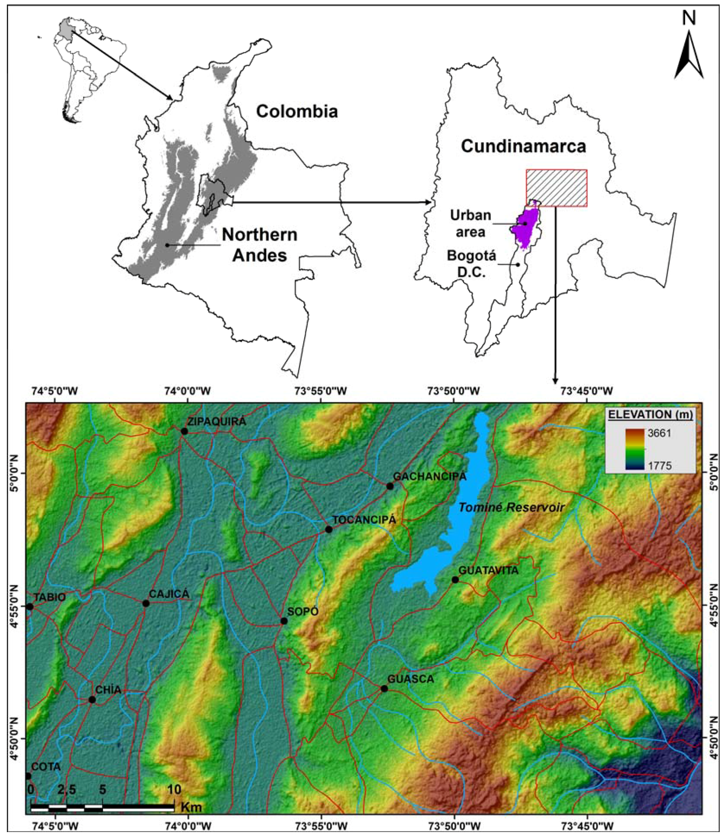
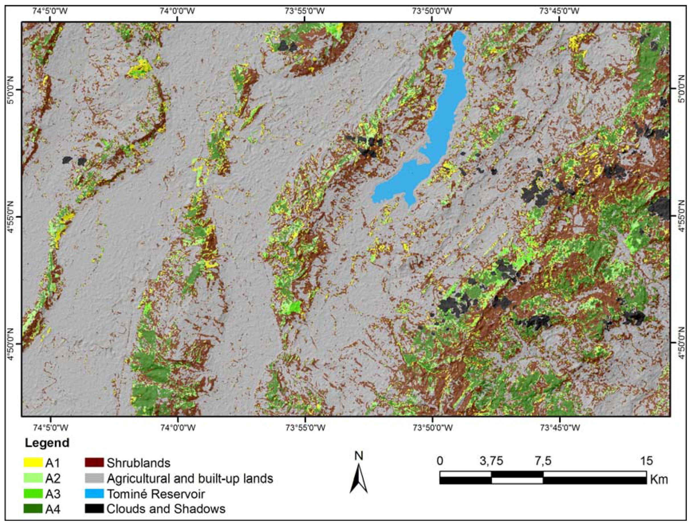
2.1. Study Area

The study area is located in a high-plain region north of Bogotá city, within the Cundinamarca Department. It encompasses about 136,000 ha and comprises a mountain plateau located in the eastern Andean cordillera, at an average altitude of 2600 m above sea level (a.s.l.). (Figure 1). The high-plain is crisscrossed by hills and mountain ranges that reach over 3500 m a.s.l. The average temperature is about 14 °C, while annual average precipitation varies from 600 mm in the center of the study area, increasing to 800–1200 mm towards the western and eastern borders respectively, with rainy seasons in April–June and September–November [27]. The region is the most densely populated in Colombia, with a population of nearly 9 million [30]. It is an important agro-industrial center of the country, with flower growing industries and dairy farming, livestock and mining being the predominant land uses [33]. The study area borders with the northern section of the capital city of Bogotá, with a population of 8 million people, and it is part of the socio-economic influence region of the city [33].
The high-plain hills/mountains are composed of Cretaceous and Tertiary shales and sandstone, whereas the plain is composed by Quaternary sediments of fluvial and lacustrine origin [34]. The native vegetation of the area comprises a variety of vegetation types and species depending on soils and climatic conditions. Original forests of the plains were dominated by species such as Quercus humboldtii, Weinmania tomentosa and Vallea stipularis [35], and mature forests hosted many species belonging to the Lauraceae family, but only small patches of intact forest remain due to logging. Nowadays, the most common and species-rich families are Melastomataceae and Ericaceae. In drier areas, one may encounter shrubs of the Morella and Myrcianthes genus. The old-growth vegetation of the hills (2700–3300 m a.s.l.) is typically dominated by trees and shrubs of the genus Weinmania, Clusia, Cedrela and Miconia [36]. From 3300 m to 3500–3600 m a.s.l., the sub-páramo prevails, a transition between forest and tropical highland grasslands dominated by shrubs and grasses belonging to the Asteraceae family (genera Espeletia and Espeletiopsis) [37].

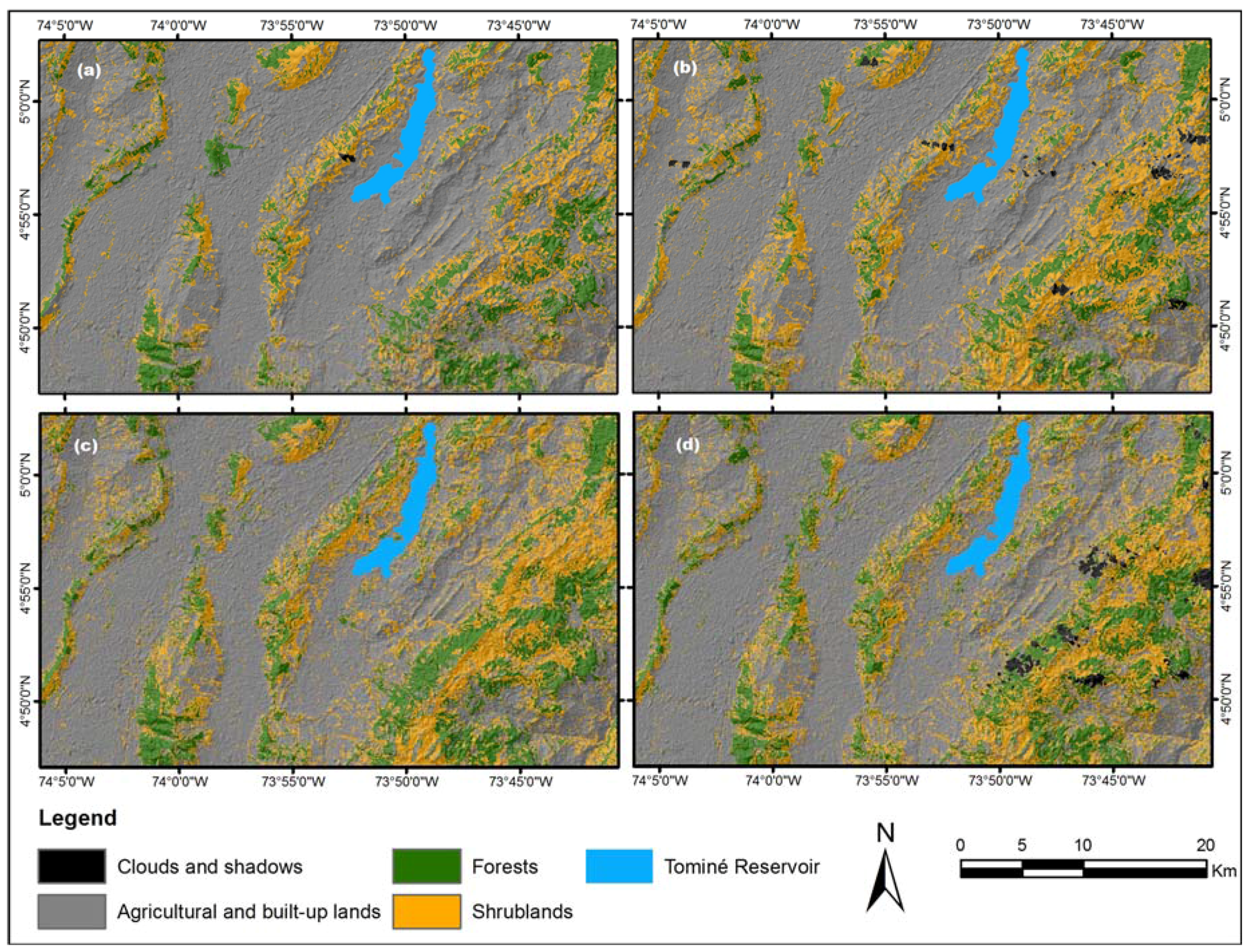
2.2. Vegetation Cover Mapping

Three Landsat TM and one Landsat OLI images were used to map recent changes in land cover. They were downloaded from the USGS Glovis server [38], spanning 30 years of landscape transformation, and corresponding to 1985, 1991, 2001 and 2015 (Table 1). The uneven length of the time intervals is due to both the difficulty of finding images with a low proportion of clouds/shadows and to errors present in the Landsat 7 ETM+ SLC-off imagery. Standard pre-processing of the images involved radiometric calibration [39] and atmospheric correction, using the Fast Line-of-sight Atmospheric Analysis of Spectral Hypercubes (FLAASH) model [40,41]. Subsequently, a parallelepiped supervised classification [42] to the subset of images corresponding to the study area for each year were used. Two main vegetation classes of interest were defined: (i) forest, which includes mature primary, secondary and planted forest; and (ii) shrub land, referring to natural shrubs and early vegetation regrowth. All the land that did not enter into these two vegetated classes of interest was merged into the agricultural and built-up lands class (ABL), which includes productive land, such as agriculture and pastureland, and built-up areas. The mapping task focused mainly on the forest and the shrubland vegetation classes. All other classes (crops, pastures and built up lands) were thus grouped into a single “agricultural and built up lands” class. In order to train the classifier, a number of training samples were defined from historical aerial imagery available in the national Colombian Geographical Institute—IGAC—for the year 1985 [43], and Google Earth historical imagery. We selected, under a simple random sampling scheme, 219, 128, 235 and 200 training points for the forest class, and 222, 125, 100 and 200 points for the shrub land vegetation class, for years 1985, 1991, 2001 and 2015, respectively. Changes in land cover areas were calculated (i) using a standard post-classification approach, and (ii) integrated by uncertainty measures (confidence intervals) of error adjusted area estimates using the methods described by Olofsson et al. [44,45] (Table S3 in Supplementary Materials).
A single mask with no land cover information was also produced by merging the classified clouds and shadows for all four years. Finally, an accuracy assessment was performed using the same sources used for training the classifier. Standard accuracy metrics were calculated using 346 (1985), 394 (2001) and 293 (2015) randomly distributed validation points. No validation points were available for 1991.

2.3. Landscape Change Analysis

To avoid underestimation of the land-cover pattern quantification due to the rugged topography of the study area, a patch area base correction was performed [46,47]. The DEM Surface Tools ArcGIS extension [48] and an ASTER Global Digital Elevation Model version 2 [49] were used to compute the surface area of each pixel based on the triangulation method proposed by Jennes [50]. Surface area for every patch and land-cover class was obtained by summing the values of its pixels [46,47].
Using the four land cover maps, transition matrices were calculated for contiguous periods of time, and for the overall period (1985–2015), based on a pixel-by-pixel comparison [51].
To identify the spatial distribution of different vegetation successional stages, we derived a ‘forest age’ map following Etter et al. [52], by assessing the presence or absence of each forest class in the classified imagery for the four dates (see Table S1 in Supplementary Material) and by establishing different forest age classes as follows (following the uneven distribution of the available images):
-
A4: ≥30 years of presence.
-
A3: 24–30 years.
-
A2: 14–24 years.
-
A1: ≤14 years.
Additionally, to describe the temporal landscape structure variation, a landscape pattern analysis was performed by computing a set of landscape metrics for the four land cover maps and the Forest Age map [53]. The analysis was carried out for each vegetation class (forest and shrub land) separately, using the Patch Analyst extension in ArcMap 10.1 (Environmental Systems Research Institute, Redlands, CA, USA). The landscape metrics selected were: number of patches (NP), mean patch size (MPS), total core area (TCA), mean core area per patch (MCAP) and core area percentage of landscape (CORLAND) [54]. NP and MPS are measures of landscape fragmentation and characterization [55], and are especially meaningful when comparing the same landscape in different time periods. TCA refers to the total amount of core area or area not affected by edge effects, MCAP refers to the distribution of the core area within the class patches, and CORLAND a measure of the dominance of the core areas in the landscape. In general, core area metrics are strongly related with the edge effect and therefore are indicators of habitat quality for many species highly dependent on core area availability [55,56].

2.4. Geographical Factors and Change

To gain an understanding of the factors that may explain the spatial dynamics in vegetation change, a multinomial linear regression model was used to evaluate the effect of environmental (soil fertility, slope) and geographical (distance to roads, distance to urban) explanatory variables on forest transitions for the 1985–2015 period [53,57]. A soil fertility map was created by establishing five fertility classes (very low, low, intermediate, high, very high) based on the national soil map [58]. The slope map was derived using the ASTER Global Digital Elevation Model version 2 [49]. Euclidean distances to roads and municipalities were calculated based on national datasets from the Planning and Land Management Geographical Information System of Colombia SIGOT [59]. All geographical layers were fitted to the 30 m raster format of the land cover maps.
Multinomial regression models generalize logistic regression to multiclass variables; that is, more than two possible discrete outcomes in the dependent variable. In other words, the transition probabilities of the different possible outcomes for each land cover class (forest, shrubland and agricultural and built-up lands) were predicted. For each land cover class, there are three possible discrete outcomes (e.g., for forests: forest to forest, forest to shrub and forest to ABL). Thus, three separate multinomial regression models for each land cover class were run to estimate the transition probabilities depending upon slope, soil fertility, distance to urban centers and distance to roads (predictive variables). In the first model, the possible outcomes of the dependent variable were forest to forest, forest to shrub and forest to ABL (n = 157,522). In the second model, the possible outcomes of the dependent variable were shrub to shrub, shrub to forest and shrub to ABL (n = 233,971). Finally, in the third model the possible outcomes of the dependent variable were agricultural and built-up lands (ABL) to ABL, ABL to forest, and ABL to shrub (n = 1,074,224).
In a second step, another multinomial linear model was built with the Forest age map, to predict the probability of vegetation cover being shrub land, young secondary forest (by merging classes A1 and A2), or late secondary and mature forest (by merging forest age classes A3 and A4) against the same predictive variables (n = 1,465,717). To deal with spatial autocorrelation, each of the models was run using a randomized subsample of 10% of the entire data set. This procedure was repeated 1000 times and the mean of each estimate was calculated, as well as the one-sided 95% confidence intervals, depending on the sign of the mean of the parameter. The multinomial models were run using the R statistical package software [60].

3. Results

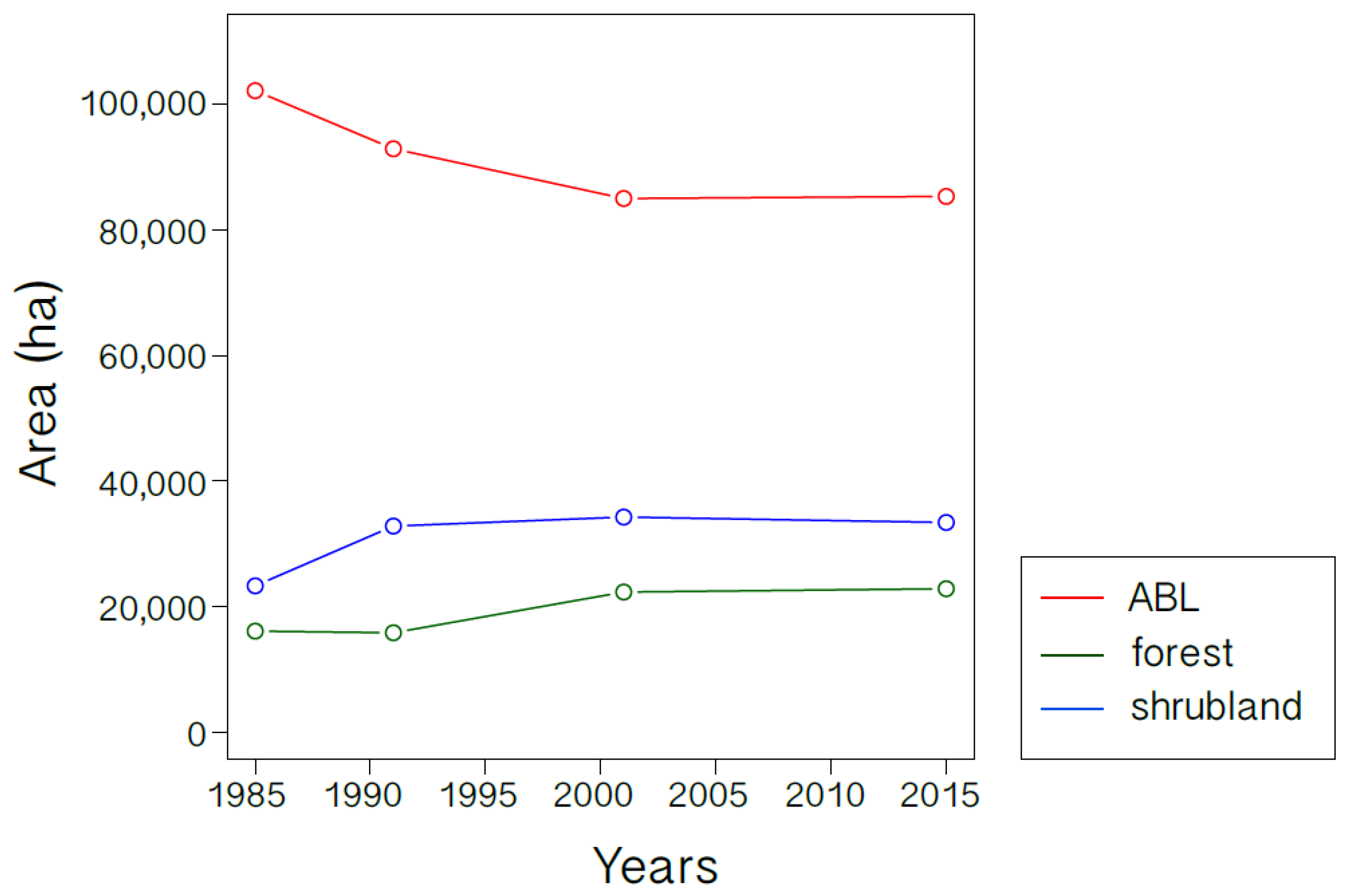
3.1. Land Cover Change Analysis

Four land cover maps, covering the years of 1985, 1991, 2001 and 2015, were produced (Figure 2). The land cover maps had overall accuracies of 89% (1985), 81.4% (2001) and 83.6% (2015). The 1991 map accuracy was not calculated due to the absence of a validation dataset for that year (Table 2 reports all accuracy measures). The analysis of 30 years of land cover changes in the Bogotá high-plain indicated a general trend of woody vegetation regrowth across the study area. The forest class increased by 42% during the study period, from 16,100 ha in 1985 to about 22,850 ha in 2015. The shrubland class also increased by a similar amount (43.3%) from 23,300 ha in 1985 to 33,400 ha in 2015. This gain in woody vegetation covers was at the expense of other land covers previously used for crops and pasture, which showed a decrease of 16,850 ha between 1985 and 2015 (−16.5%). The intermediate period between 1991 and 2001 was characterized by the strongest trend of forest regrowth, while the period 2001–2015 showed a stabilization in land cover change (Figure 3). The most frequent transition in the whole study period was from shrubland to forest, indicating an important process of forest recovery. In contrast, the shrubland class showed a high degree of change, both toward recovery or toward loss (Table 3). Land cover error-adjusted area estimates with 95% confidence intervals are reported in Table S3 (Supplementary Materials, using methods from [44,45]). Overall land cover changes (1985–2015) were spatially represented by nine different land cover transitions (Figure 4.)
Altitudinal changes were also analyzed. The most stable areas of shrub lands and forests were found at altitudes over 2800 m (Figure 5). The altitude belt over 2600 m was the most dynamic, showing a strong increase in forest and shrubland areas. On the other hand, around 50% of the agricultural and built-up lands (ABL) in 1985 below 2600 m remained stable over the study period (Figure 5).

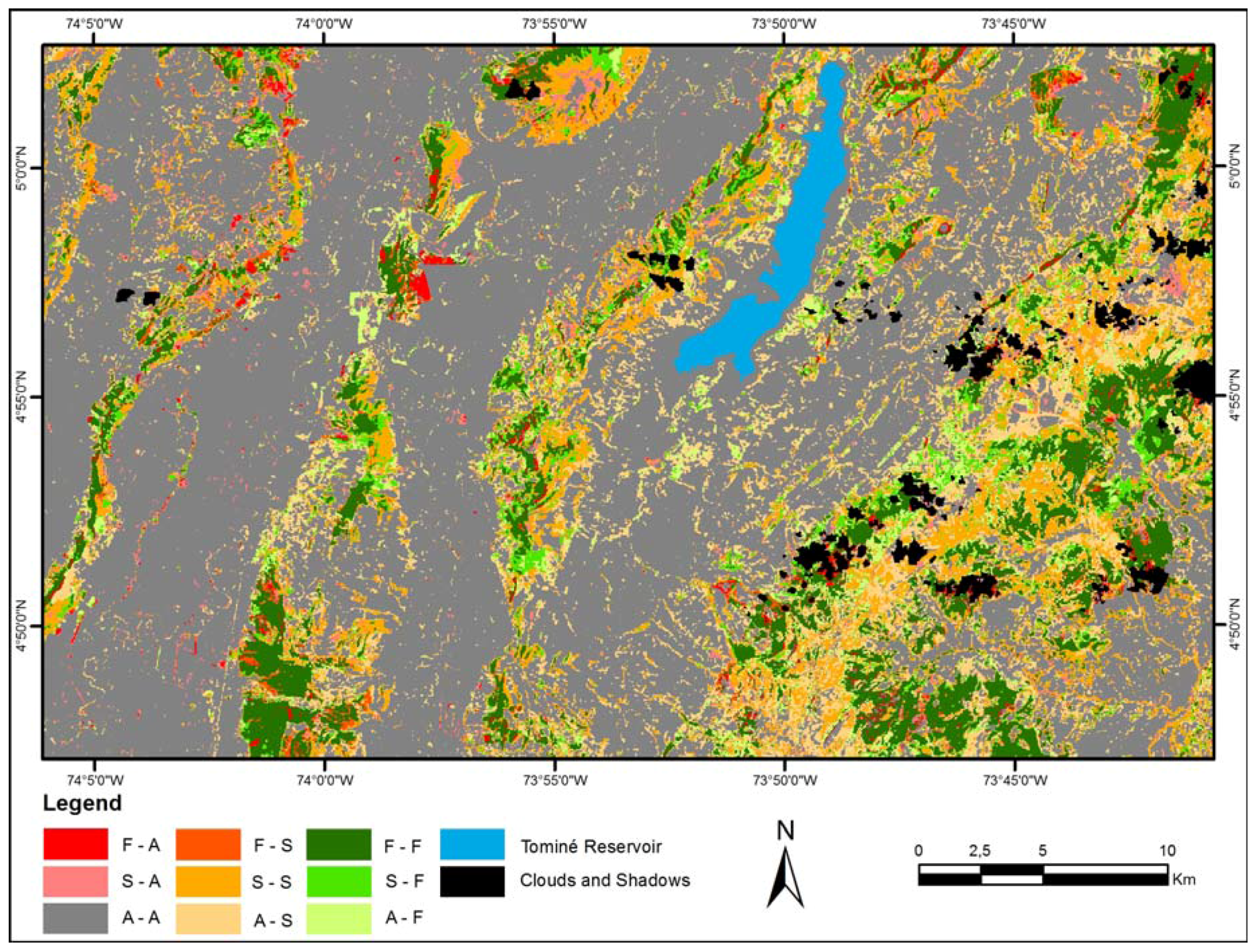
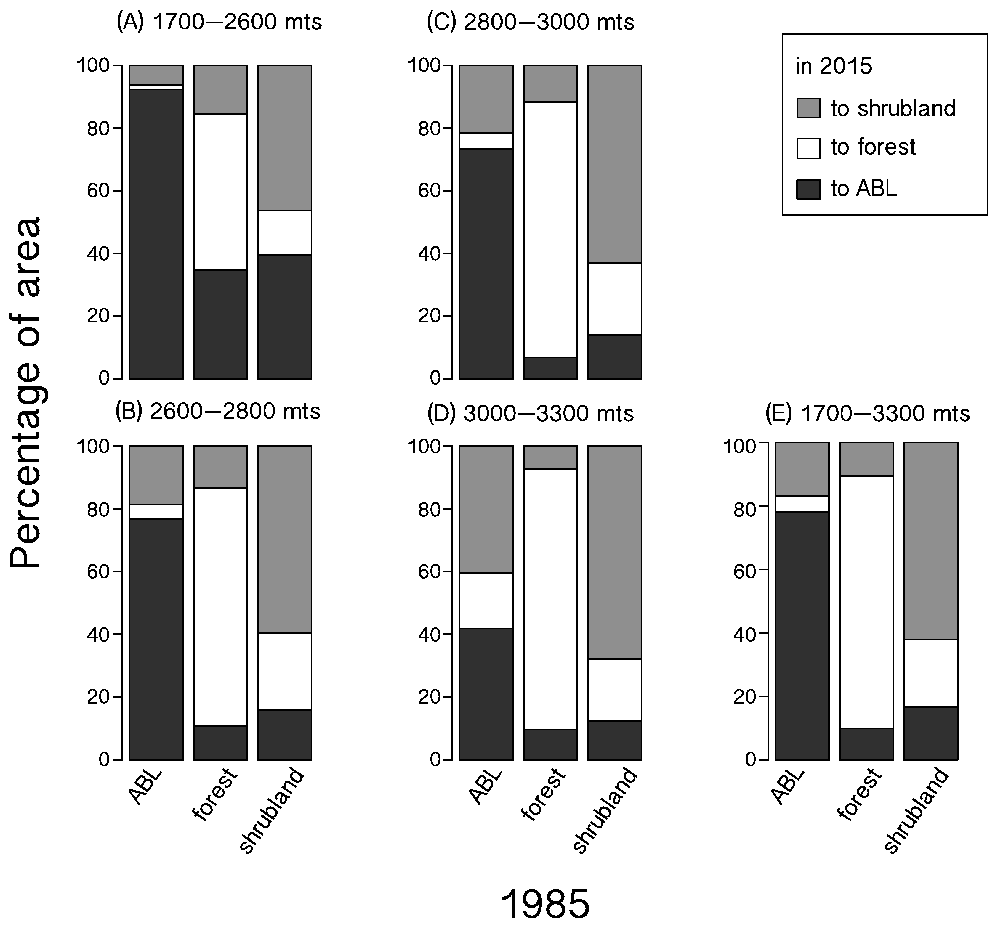
3.2. Patterns of Landscape Change

About 45% of forest cover remained stable over the study period (forest age class A4). These older secondary forests are located in the highest elevations and steeper slopes, where anthropogenic disturbance is less likely and where less fertile soils are found. Young secondary forests (forest age classes A1 and A2; Table S2) were more common at lower altitudes, where land cover change is more dynamic. Forest regrowth occurred to a large extent in the western part of the study area (Figure 6).
Land cover change processes had a large influence on the spatial structure of woody vegetated areas, showing an overall increase in the number of forest patches, resulting from a scattered pattern of forest regrowth. Mean patch size (MPS) and mean core area (MCA) oscillated in size during the study period, yet forest patches showed a notable decrease in size in 2015 compared to 1985. The number of forest patches belonging to age class A4 (≥30 years of presence) was lower than that of younger secondary forests (age classes A1 to A3; i.e., ≤30 years of presence), and showed a higher mean patch size and mean core areas. For the shrubland class, the number of patches also increased over time, as well as their mean patch size and core area (Table 4).

3.3. Landscape Change Correlates

The regression models for land cover transitions during the study period showed clear opposite trend processes related to land clearing (forest or shrubland to agricultural and built-up lands) and those related to woody vegetation regrowth (agricultural and built-up lands to forest or to shrubland). As expected, distance to roads and to urban centers showed a strong effect on land cover dynamics. The nearer to urban centers and roads, the more forest areas were likely to become shrubs or agricultural and built-up lands by 2015. Likewise, shrubs were more likely to become forests or ABL lands than to remain stable. In contrast, ABL lands in 1985 were more likely to remain stable when they were near urban centers and roads (Table 5).
Environmental variables also appeared to affect land cover change. Steep slopes favored persistence and gain of woody vegetation cover. The steeper the slope, the less likely were forests to become shrubs and shrubs to become cleared; and agricultural and built-up lands were more likely to become shrubs or forests. Fertile soils showed higher dynamic. Here, forests were more likely to become shrubs or ABL lands, than to remain forests. Likewise, shrublands were more likely to become forests or ABL lands. In contrast, less fertile soils were more likely to show shrublands and forest regrowth (Table 5).
The forest age model showed that all woody vegetation (forest and shrubland classes) was more likely to be present far from urban centers and roads, on steeper slopes, and on fertile soils. These effects were stronger for forest age classes A3 and A4. In addition, shrublands and young secondary forests (<24 years old) were scarcer in fertile soils (Table 6).

4. Discussion

Although this landscape has been highly transformed for a long time [26], it continues to show strong dynamics driven by an apparent land use dis-intensification and land abandonment in the mountains and hills of the region. Overall, this study shows two important aspects: (i) a general increasing trend in woody cover, and (ii) although land cover changes strongly varied between periods and between altitudinal belts, the period 1991–2001, and above 2800 m, was dominated by woody cover increase. The abandonment of agricultural and built-up lands and shrublands followed a successional process, resulting in increasing areas of young or intermediate secondary forests across the landscape. These findings support previous studies showing that forest cover is increasing in the southwest of the Bogotá high-plain region [27], and is consistent with the trend of woody vegetation recovery reported for Colombia at the national level during the last decade [28]. Indeed, net gains in forest cover have also been observed in several other areas of Latin America and the Caribbean (e.g., [61,62,63,64]). These patterns have been associated with rural-to-urban-migration dynamics, which reduce the pressure to convert forest patches, and promote forest regrowth through land abandonment [65,66]. By providing increased labor opportunities and access to higher education, urban centers have become very attractive to rural populations.
Despite the fact that 45% of the forested areas remained stable during the study period, the study found considerable dynamics in many forest and shrubland patches. Young secondary forests increased in area, but mostly in a pattern of small and disconnected patches, mainly in lower elevations and accessible areas. Forests that were already present at the beginning of the study period represent only a small fraction of areas covered by woody vegetation in the study area. However, these patches have the largest mean core area and mean patch size, and represent remnants of the forests covering the whole area in the past. This is remarkable as most Andean slopes in this region were strongly deforested a century ago as a result of cropping activities, cattle grazing [26], and because wood was a critical source of cooking energy during the early 20th century [67]. If these remnant forests indeed correspond to old-growth forests, they should harbor considerable levels of biodiversity, and could therefore be used as core areas to implement a protected areas network that can integrate the increasing areas of regrowth forests to shield against the high conversion risks [28,68].
During the study period, the number of patches of forest vegetation increased, but both mean patch area and mean core area decreased. These seemingly contradictory trends may be the result of two processes occurring simultaneously. First, the proliferation of patches indicates that vegetation regrowth is taking over after land abandonment which may be associated with soil productivity loss, economic marginalization and/or agriculture intensification [4,65]. Second, the decline in mean patch and core area probably results from the process of fragmentation associated with land conversion, which is still underway, with some smaller areas converted to productive lands. Size reduction in forest patches may also be the result of activities related with residential construction and industrial development [69], often occurring in peri-urban areas [70]. Future studies evaluating vegetation stand dynamics at the local scale can help clarify this issue.
Regression analyses showed that landscape variables had an important effect on forest transitions. First, the study found that there is an important dynamic towards both forest regrowth and clearing near urban centers and roads. Other theoretical and empirical studies have shown that deforestation processes are more likely to occur in accessible areas, while forest regrowth typically takes place in less accessible ones [71,72,73,74,75,76]. Patterns of recovery near urban areas and roads may be explained by the increase of low-density suburban settlements of secondary homes of people living in Bogotá, well represented in the area, who are promoting forest regeneration within their properties. Another possibility is that access to roads is positively related to land cover change dynamics. In other words, transitions to forests or to shrublands near roads or urban centers could be the result of previously cleared lands where vegetation is now restoring, but that is likely to be become agricultural or built-up land in the near future. In 2015, however, woody vegetation was more likely to be found far from urban centers and roads. Together, these findings suggest that, although areas close to urban centers may be associated to some extent of forest regrowth, the larger fraction of forest cover, especially of older forest age classes, is found far from human settlements.
Along with human settlements, fertile soils also turned out to be a key driver of both forest recovery and degradation simultaneously. Although mature remnant forests were found in more fertile soils, which is somewhat counterintuitive, they are associated also with steeper slopes and are far from roads and settlements. In turn, regrowth forests occur on less fertile soils, which are more likely to be abandoned. Regrowth also occurs on steeper slopes and further away from roads and settlements. Indeed, soil fertility is widely recognized as a driver of either deforestation or forest succession [77,78], as it acts as a land use regulator by determining the agricultural value and economic potential of an area. For instance, forests occurring on fertile soils are more likely to undergo conversion towards farming, while converted lands on less fertile soils are more likely to be abandoned, allowing succession to result in new secondary forests [65]. Also, some forest patches may have remained intact for several decades as they are often located at the top edge of mountains and along steep cliffs. Another possibility is that of an increased consciousness of the local populations about the biodiversity value and the ecosystem services provided by forest cover [32]. In marginal areas with steep slopes, forests were more stable, and agricultural and built-up lands were more likely to become shrubs or forests. This is in agreement with Mendoza and Etter [27], who found that more than 70% of the remnant forests were located in areas with slopes over 25%.
Finally, these results raise new research questions that need to be further investigated at both local and regional scales. In particular, it is critical to evaluate forest resilience. Although the ecological value of secondary forests has grown in the last decade as a result of a global decrease of primary forests [79], floristic reassembly is a very slow process, and the original species composition may never return to its original state [80,81]. For instance, many secondary forests in the region are dominated by Ulex europaeus, an invasive species prone to fire, which is very likely to replace native species, and is difficult to eradicate [82]. Also, shrublands are an important component of the current landscape, which raises the question whether these correspond to vegetation which is gradually recovering from strong past disturbances, or whether they represent an arrested successional stage owing to soil degradation and/or seed limitation [83]. In this context, future research should involve more detailed studies in the Bogota high-plain, comparing the successional dynamics among shrubland and early and late secondary forests in different fragmentation scenarios. Andean forests hold key ecosystems with the potential of being important biodiversity reservoirs and of providing important ecosystem services related to water regulation and carbon sequestration [84]. Historically, much attention has been given to tropical lowland rainforests. Here, the importance to broaden ecological research to these less studied tropical ecosystems is stressed, where our knowledge about carbon and water budgets is still limited [84].
Some limitations of the research derive from the absence of validation points for the 1991 land cover map. Additionally, measures of error adjusted areas and relative confidence intervals should have been calculated also for the land cover change transition matrix (1985–2015) [44,45], which was not possible due to the absence of an ad-hoc change validation dataset. Finally, the study covered only part of the northern region neighboring Bogotá; further analysis to corroborate the generality of our conclusions should involve research in additional areas of the Bogotá high-plain.

5. Conclusions

Evidence of an important forest recovery process in a surrounding area of the city of Bogotá, a large urban region of the Eastern Colombian Andes, is provided. Although we may be optimistic about the future of forest cover recovery in the Andean region, our findings also reflect the complexity of the processes occurring in such a highly transformed and densely populated region, where the same factor can be a driver of both deforestation and recovery simultaneously. Overall, our results bring noteworthy elements to the understanding of the factors driving land cover change in large peri-urban areas, which greatly benefit from the environmental services that surrounding forest cover provides. A deeper understanding of the drivers of land cover change in these ecosystems is crucial for the design of regional environmental plans that can direct more sustainable settlement models, enhance conservation initiatives and improve the delivery of ecosystem services.

Supplementary Materials

The following are available online at www.mdpi.com/1999-4907/8/6/216/s1, Table S1: Forest age class definition (1 = presence of forest, 0 = absence). Table S2: Forest age classes extensions in 2015. Table S3: Error-adjusted area estimates and 95% confidence intervals (CI), following [44,45].

Acknowledgments

The research work was supported by institutional funding from the Pontificia Universidad Javeriana and the Universidad del Rosario. The Authors would like to acknowledge the US Geological Survey (USGS) and the US National Aeronautics and Space Administration (NASA) for providing the Landsat images. Anonymous colleagues are also acknowledged for insightful discussions about the paper.

Author Contributions

K.R., A.E., N.N. and N.C. conceived and designed the experiments; K.R. and N.N. performed the experiments; K.R., N.N., N.C. and A.E. analyzed the data; K.R., N.C., N.N. and A.E. wrote the paper.

Conflicts of Interest

The authors declare no conflict of interest. The founding sponsors had no role in the design of the study; in the collection, analyses, or interpretation of data; in the writing of the manuscript, and in the decision to publish the results.

References

  1. Roberts, L. 9 Billion? Science 2011, 333, 540–543. [Google Scholar] [CrossRef] [PubMed]
  2. Grimm, N.B.; Faeth, S.H.; Golubiewski, N.E.; Redman, C.L.; Wu, J.; Bai, X.; Briggs, J.M. Global change and the ecology of cities. Science 2008, 319, 756–760. [Google Scholar] [CrossRef] [PubMed]
  3. Lambin, E.F.; Geist, H.J. Land-Use and Land-Cover Change: Local Processes and Global Impacts; Springer: Berlin, Germany, 2006. [Google Scholar]
  4. Foley, J.A.; DeFries, R.; Asner, G.P.; Barford, C.; Bonan, G.; Carpenter, S.R.; Chapin, F.S.; Coe, M.T.; Daily, G.C.; Gibbs, H.K.; et al. Global consequences of land use. Science 2005, 309, 570–574. [Google Scholar] [CrossRef] [PubMed]
  5. Lambin, E.F.; Geist, H.J.; Lepers, E. Dynamics of land-use and land-cover change in tropical regions. Annu. Rev. Environ. Resour. 2003, 28, 205–241. [Google Scholar] [CrossRef]
  6. Millennium Ecosystem Assessment. Ecosystems and Human Well-Being: Synthesis; Island Press: Washington, DC, USA, 2005. [Google Scholar]
  7. Vitousek, P.M.; Mooney, H.A.; Lubchenco, J.; Melillo, J.M. Human domination of Earth’s ecosystems. Science 1997, 277, 494–499. [Google Scholar] [CrossRef]
  8. Intergovernmental Panel on Climate Change (IPCC). Climate Change 2013: The Physical Science Basis. Contribution of Working Group I to the Fifth Assessment Report of the Intergovernmental Panel on Climate Change, 1st ed.; Cambridge University Press: New York, NY, USA, 2013. [Google Scholar]
  9. Mahmood, R.; Pielke, R.A.; Hubbard, K.G.; Niyogi, D.; Dirmeyer, P.A.; McAlpine, C.; Carleton, A.M.; Hale, R.; Gameda, S.; Beltrán-Przekurat, A.; et al. Land cover changes and their biogeophysical effects on climate. Int. J. Climatol. 2014, 34, 929–953. [Google Scholar] [CrossRef]
  10. Uriarte, M.; Schneider, L.; Rudel, T.K. Synthesis: Land transitions in the tropics. Biotropica 2010, 42, 59–62. [Google Scholar] [CrossRef]
  11. Orme, C.D.L.; Davies, R.G.; Burgess, M.; Eigenbrod, F.; Pickup, N.; Olson, V.A.; Webster, A.J.; Ding, T.-S.; Rasmussen, P.C.; Ridgely, R.S.; et al. Global hotspots of species richness are not congruent with endemism or threat. Nature 2005, 436, 1016–1019. [Google Scholar] [CrossRef] [PubMed]
  12. Grau, H.R.; Aide, T.M. Globalization and land-use transitions in Latin America. Ecol. Soc. 2008, 13, 16–27. [Google Scholar] [CrossRef]
  13. Ahmed, S.E.; Souza, C.M., Jr.; Ribeiro, J.; Ewers, R.M. Temporal patterns of road network development in the Brazilian Amazon. Reg. Environ. Chang. 2013, 13, 927–937. [Google Scholar] [CrossRef]
  14. Fraser, B. Deforestation: Carving up the Amazon. Nature 2014, 509, 418–419. [Google Scholar] [CrossRef] [PubMed]
  15. Achard, F.; Eva, H.D.; Stibig, H.-J.; Mayaux, P.; Gallego, J.; Richards, T.; Malingreau, J.-P. Determination of deforestation rates of the world's humid tropical forests. Science 2002, 297, 999–1002. [Google Scholar] [CrossRef] [PubMed]
  16. Achard, F.; Beuchle, R.; Mayaux, P.; Stibig, H.-J.; Bodart, C.; Brink, A.; Carboni, S.; Descleé, B.; Donnay, F.; Eva, H.D.; et al. Determination of tropical deforestation rates and related carbon losses from 1990 to 2010. Glob. Chang. Biol. 2014, 20, 2540–2554. [Google Scholar] [CrossRef] [PubMed]
  17. Laurance, W.F. Have we overstated the tropical biodiversity crisis? Trends Ecol. Evol. 2007, 22, 65–70. [Google Scholar] [CrossRef] [PubMed]
  18. Salazar, A.; Baldi, G.; Hirota, M.; Syktus, J.; McAlpine, C. Land use and land cover change impacts on the regional climate of non-Amazonian South America: A review. Glob. Planet. Chang. 2015, 128, 103–119. [Google Scholar] [CrossRef]
  19. Hansen, M.C.; Potapov, P.V.; Moore, R.; Hancher, M.; Turubanova, S.A.; Tyukavina, A.; Thau, D.; Stehman, S.V.; Goetz, S.J.; Loveland, T.R.; et al. High-Resolution Global Maps of 21st-Century Forest Cover Change. Science 2013, 342, 850–853. [Google Scholar] [CrossRef] [PubMed]
  20. Myers, N.; Mittermeier, R.A.; Mittermeier, C.G.; da Fonseca, G.A.B.; Kent, J. Biodiversity hotspots for conservation priorities. Nature 2000, 403, 853–858. [Google Scholar] [CrossRef] [PubMed]
  21. Romero, M.; Cabrera, E.; Ortiz, N. Informe Sobre el Estado de la Biodiversidad en Colombia 2006–2007; Instituto de Investigación de Recursos Biólogicos Alexander von Humboldt: Bogotá D.C., Colombia, 2008. [Google Scholar]
  22. Etter, A.; van Wyngaarden, W. Patterns of landscape transformation in Colombia, with emphasis in the Andean region. AMBIO 2000, 29, 432–439. [Google Scholar] [CrossRef]
  23. Cavelier, J.; Etter, A. Deforestation of montane forests in Colombia as a result of illegal opium plantations (Papaver somniferum). In Biodiversity and Conservation of Neotropical Montane Forests; Churchill, S.P., Balslev, H., Forero, E., Luteyn, J.L., Eds.; The New York Botanical Garden: New York, NY, USA, 1995; pp. 541–550. [Google Scholar]
  24. Chadid, M.A.; Dávalos, L.M.; Molina, J.; Armenteras, D. A Bayesian Spatial Model Highlights Distinct Dynamics in Deforestation from Coca and Pastures in an Andean Biodiversity Hotspot. Forests 2015, 6, 3828–3846. [Google Scholar] [CrossRef]
  25. Sánchez-Cuervo, A.M.; Aide, T.M. Consequences of the armed conflict, forced human displacement, and land abandonment on forest cover change in Colombia: A multi-scale analysis. Ecosystems 2013, 16, 1052–1070. [Google Scholar] [CrossRef]
  26. Etter, A.; McAlpine, C.; Possingham, H. Historical patterns and drivers of landscape change in Colombia since 1500: A regionalized spatial approach. Ann. Assoc. Am. Geogr. 2008, 98, 2–23. [Google Scholar] [CrossRef]
  27. Mendoza, J.E.; Etter, A. Multitemporal analysis (1940–1996) of land cover changes in the southwestern Bogotá High-plain. Landsc. Urban Plan. 2002, 59, 147–158. [Google Scholar] [CrossRef]
  28. Sánchez-Cuervo, A.M.; Aide, T.M.; Clark, M.L.; Etter, A. Land Cover Change in Colombia: Surprising Forest Recovery Trends between 2001 and 2010. PLoS ONE 2012, 7, e43943. [Google Scholar] [CrossRef] [PubMed]
  29. Norden, N.; Chazdon, R.L.; Chao, A.; Jiang, Y.-H.; Vílchez-Alvarado, B. Resilience of tropical rain forests: Tree community reassembly in secondary forests. Ecol. Lett. 2009, 12, 385–394. [Google Scholar] [CrossRef] [PubMed]
  30. Departamento Administrativo Nacional de Estadística (DANE). Available online: http://www.dane.gov.co/ (accessed on 15 October 2015).
  31. Secretaría Distrital de Planeación. Región Metropolitana de Bogotá: Una Visión de la Ocupación del Suelo; Alcaldía Mayor de Bogotá D.C.: Bogotá D.C., Colombia, 2014.
  32. Etter, A.; Villa, L.A. Andean forest and farming systems in part of the eastern cordillera (Colombia). Mt. Res. Dev. 2000, 20, 236–245. [Google Scholar] [CrossRef]
  33. Antonio-Fragala, F.; Obregón-Neira, N. Recharge estimation in aquifers of the Bogotá Savannah. Ing. Univ. 2011, 15, 145–169. [Google Scholar]
  34. Saldarriaga, A. Hubo una vez una Sabana: Aproximación al Estudio de la Transformación de la Sabana de Bogotá; Instituto Geográfico Agustín Codazzi: Bogotá D.C., Colombia, 1974.
  35. Van der Hammen, T. La sabana de Bogotá y su lago en el Pleniglacial Medio. Caldasia 1986, 15, 249–262. [Google Scholar]
  36. Cortés-S, S.P.; Van der Hammen, T.; Rangel-Ch, J.O. Comunidades vegetales y patrones de degradación y sucesión en la vegetación de los Cerros Occidentales de Chía-Cundinamarca-Colombia. Rev. Acad. Colomb. Cienc. 1999, 23, 529–554. [Google Scholar]
  37. Van der Hammen, T. Plan Ambiental de la Cuenca Alta del río Bogotá: Análisis y Orientación Para el Ordenamiento Territorial; CAR: Bogotá D.C., Colombia, 1998. [Google Scholar]
  38. United States Geological Survey. USGS Global Visualization Viewer. Available online: http://glovis.usgs.gov/ (accessed on 3 August 2015).
  39. Chander, G.; Markham, B.L.; Helder, D.L. Summary of current radiometric calibration coefficients for Landsat MSS, TM, ETM+, and EO-1 ALI sensors. Remote Sens. Environ. 2009, 113, 893–903. [Google Scholar] [CrossRef]
  40. Berk, A.; Bernstein, L.S.; Anderson, G.P.; Acharya, P.K.; Robertson, D.C.; Chetwynd, J.H.; Adler-Golden, S.M. MODTRAN Cloud and Multiple Scattering Upgrades with Application to AVIRIS. Remote Sens. Environ. 1998, 65, 367–375. [Google Scholar] [CrossRef]
  41. Matthew, M.W.; Addler-Golden, S.M.; Berk, A.; Richtsmeier, S.C.; Levine, R.Y.; Bernstein, L.S.; Acharya, P.K.; Anderson, G.P.; Felde, G.W.; Hoke, M.L.; et al. Status of Atmospheric Correction Using a MODTRAN4-based Algorithm. SPIE Proc. SPIE VI 2000, 4049, 99–207. [Google Scholar]
  42. Richards, J.A.; Xiuping, J. Remote Sensing Digital Image Analysis, 3rd ed.; Springer: Berlin/Heidelberg, Germany, 1999. [Google Scholar]
  43. Instituto Geográfico Agustín Codazzi (IGAC). Aerial Images 267, 269, Embalse de Tominé, Guatavita, Cundinamarca, Flight C-2275, 1985; Instituto Geográfico Agustín Codazzi: Bogotá, D.C., Colombia, 1985.
  44. Olofsson, P.; Foody, G.M.; Stehman, S.V.; Woodcock, C.E. Making better use of accuracy data in land change studies: Estimating accuracy and area and quantifying uncertainty using stratified estimation. Remote Sens. Environ. 2013, 129, 122–131. [Google Scholar] [CrossRef]
  45. Olofsson, P.; Foody, G.M.; Herold, M.; Stehman, S.V.; Woodcock, C.E.; Wulder, M.A. Good practices for estimating area and assessing accuracy of land change. Remote Sens. Environ. 2014, 148, 42–57. [Google Scholar] [CrossRef]
  46. Hoechstetter, S.; Walz, U.; Dang, L.H.; Thinh, N.X. Effects of topography and surface roughness in analyses of landscape structure—A proposal to modify the existing set of landscape metrics. Landsc. Online 2008, 1, 1–14. [Google Scholar] [CrossRef]
  47. Zhiming, Z.; van Coillie, F.; De Wulf, R.; De Clercq, E.V.; Xiaokun, O. Comparison of surface and planimetric landscape metrics for mountainous land cover pattern quantification in Lancang watershed, China. Mt. Res. Dev. 2012, 32, 213–225. [Google Scholar] [CrossRef]
  48. Jennes, J. DEM Surface Tools; Jennes Enterprises: Flagstaf, AZ, USA, 2013; Available online: http://www.jennessent.com/arcgis/surface_area.htm (accessed on 21 October 2015).
  49. Hayakawa, Y.S.; Oguchi, T.; Lin, Z. Comparison of new and existing global digital elevation models: ASTER G-DEM and SRTM-3. Geophys. Res. Lett. 2008, 35, 1–5. [Google Scholar] [CrossRef]
  50. Jennes, J. Calculating landscape surface area from digital elevation models. Wildlife Soc. B 2004, 32, 829–839. [Google Scholar] [CrossRef]
  51. Colditz, R.R.; Acosta-Velázquez, J.; Díaz Gallegos, J.R.; Vázquez Lule, A.D.; Rodríguez-Zúñiga, M.T.; Maeda, P.; Cruz López, M.I.; Ressl, R. Potential effects in multi-resolution post-classification change detection. Int. J. Remote Sens. 2012, 33, 6426–6445. [Google Scholar] [CrossRef]
  52. Etter, A.; McAlpine, C.; Pullar, D.; Possingham, H. Modelling the age of tropical moist forest fragments in heavily-cleared lowland landscapes of Colombia. For. Ecol. Manag. 2005, 298, 249–260. [Google Scholar] [CrossRef]
  53. Gillanders, S.N.; Coops, N.C.; Wulder, M.A.; Gergel, S.E.; Nelson, T. Multitemporal remote sensing of landscape dynamics and pattern change: Describing natural and anthropogenic trends. Prog. Phys. Geogr. 2008, 32, 503–528. [Google Scholar] [CrossRef]
  54. Cushman, S.A.; McGarigal, K.; Neel, M.C. Parsimony in landscape metrics: Strength, universality, and consistency. Ecol. Indic. 2008, 8, 691–703. [Google Scholar] [CrossRef]
  55. McGarigal, K. Fragstats 4.2 Help; University of Massachusetts: Amherst, MA, USA, 2013. [Google Scholar]
  56. Parra Sánchez, E.; Armenteras, D.; Retana, J. Edge Influence on Diversity of Orchids in Andean Cloud Forests. Forests 2016, 7, 63. [Google Scholar] [CrossRef]
  57. Etter, A.; McAlpine, C.; Wilson, K.; Phinn, S.; Possingham, H. Regional patterns of agricultural land use and deforestation in Colombia. Agric. Ecosyst. Environ. 2006, 114, 369–386. [Google Scholar] [CrossRef]
  58. IGAC. Soil Map of Colombia; Subdirección de Agrología: Bogotá D.C., Colombia, 2014. Available online: http://geoportal.igac.gov.co:8888/siga_sig/Agrologia.seam (accessed on 26 October 2015).
  59. IGAC. Planning and Land Management Geographical Information System of Colombia (SIGOT). Available online: http://sigotn.igac.gov.co (accessed on 23 September 2015).
  60. R Core Team. R: A Language and Environment for Statistical Computing. R Foundation for Statistical Computing: Vienna, Austria. Available online: https://www.R-project.org/ (accessed on 10 May 2017).
  61. Aide, T.M.; Clark, M.L.; Grau, H.R.; López-Carr, D.; Levy, M.A.; Redo, D.; Bonilla-Moheno, M.; Riner, G.; Andrade-Núñez, M.J.; Muñiz, M. Deforestation and reforestation of Latin America and the Caribbean (2001–2010). Biotropica 2013, 45, 262–271. [Google Scholar] [CrossRef]
  62. Grau, H.R.; Aide, T.M.; Zimmerman, J.K.; Thomlinson, J.R.; Helmer, E.; Zou, X. The ecological consequences of socioeconomic and land-use changes in postagriculture Puerto Rico. Bioscience 2003, 53, 1159–1168. [Google Scholar] [CrossRef]
  63. Hecht, S.B.; Kandel, S.; Gomes, I.; Cuellar, N.; Rosa, H. Globalization, forest resurgence, and environmental politics in El Salvador. World Dev. 2006, 34, 308–323. [Google Scholar] [CrossRef]
  64. Rudel, T.K.; Bates, D.; Machinguiashi, R. A tropical forest transition? Agricultural change, out-migration, and secondary forests in the Ecuadorian Amazon. Ann. Assoc. Am. Geogr. 2002, 92, 87–102. [Google Scholar] [CrossRef]
  65. Aide, T.M.; Grau, H.R. Globalization, migration and Latin American ecosystems. Science 2004, 305, 1915–1916. [Google Scholar] [CrossRef] [PubMed]
  66. Wright, S.J.; Muller-Landau, H.C. The future of tropical forest species. Biotropica 2006, 38, 287–301. [Google Scholar] [CrossRef]
  67. Meza, C.A. Encrucijada y conflicto. Urbanización, conservación y ruralidad en los cerros orientales de Bogotá. Rev. Colomb. Antropol. 2008, 44, 439–480. [Google Scholar]
  68. Harper, K.A.; Macdonald, S.E.; Burton, P.J.; Chen, J.; Brosofke, K.D.; Saunders, S.C.; Euskirchen, E.S.; Roberts, D.; Jaiteh, M.S.; Esseen, P.-A. Edge influence on forest structure and composition in fragmented landscapes. Conserv. Biol. 2005, 19, 768–782. [Google Scholar] [CrossRef]
  69. Fischer, J.; Lindenmayer, D.B. Landscape modification and habitat fragmentation: A synthesis. Glob. Ecol. Biogeogr. 2007, 16, 265–280. [Google Scholar] [CrossRef]
  70. Antrop, M. Landscape change and the urbanization process in Europe. Landsc. Urban Plan. 2004, 67, 9–26. [Google Scholar] [CrossRef]
  71. Ludeke, A.K.; Maggio, R.C.; Reid, L.M. An analysis of anthropogenic deforestation using logistic regression and GIS. J. Environ. Manag. 1990, 31, 247–259. [Google Scholar] [CrossRef]
  72. Munroeaic, D.K.; Southworth, J.; Tucker, C.M. The dynamics of land-cover change in western Honduras: Exploring spatial and temporal complexity. Agric. Econ. 2002, 27, 355–369. [Google Scholar] [CrossRef]
  73. Nepstad, D.; Carvalho, G.; Barros, A.C.; Alencar, A.; Capobianco, J.P.; Bishop, J.; Moutinho, P.; Lefebvre, P.; Silva, U.L., Jr.; Prins, E. Road paving, fire regime feedbacks, and the future of Amazon forests. For. Ecol. Manag. 2001, 154, 395–407. [Google Scholar] [CrossRef]
  74. Pfaff, A.S.P. What drives deforestation in the Brazilian Amazon? Evidence from satellite and socioeconomic data. J. Environ. Econ. Manag. 1999, 37, 26–43. [Google Scholar] [CrossRef]
  75. Read, J.M.; Denslow, J.S.; Guzman, S.M. Documenting land cover history of a humid tropical environment in northeastern Costa Rica using time-series remotely sensed data. In GIS and Remote Sensing Applications in Biogeography and Ecology; Millington, A.C., Walsh, S.J., Osborne, P.E., Eds.; Kluwer Academic Publishers: Boston, MA, USA, 2001; pp. 69–89. [Google Scholar]
  76. Soares-Filho, B.S.; Assunção, R.M.; Pantuzzo, A.E. Modeling the spatial transition probabilities of landscape dynamics in an Amazonian colonization frontier. Bioscience 2001, 51, 1059–1067. [Google Scholar] [CrossRef]
  77. Moran, E.F.; Brondizio, E.S.; Tucker, J.M.; da Silva-Forsberg, M.C.; McCracken, S.; Falesi, I. Effects of soil fertility and land-use on forest succession in Amazonia. For. Ecol. Manag. 2000, 139, 93–108. [Google Scholar] [CrossRef]
  78. Veldkamp, E.; Weitz, A.M.; Staritsky, I.G.; Huising, E.J. Deforestation trends in the Atlantic zone of Costa Rica: A case study. Land Degrad. Dev. 1992, 3, 71–84. [Google Scholar] [CrossRef]
  79. Chazdon, R.L. Second Growth: The Promise of Tropical Forest Regeneration in an Age of Deforestation; University of Chicago Press: Chicago, IL, USA, 2014. [Google Scholar]
  80. Norden, N.; Mesquita, R.C.; Bentos, T.V.; Chazdon, R.L.; Williamson, G.B. Contrasting community compensatory trends in alternative successional pathways in central Amazonia. Oikos 2011, 120, 143–151. [Google Scholar] [CrossRef]
  81. Turner, I.M.; Wong, Y.K.; Chew, P.T.; bin Ibrahim, A. Tree species richness in primary and old secondary tropical forest in Singapore. Biodivers. Conserv. 1997, 6, 537–543. [Google Scholar] [CrossRef]
  82. Gómez-Ruiz, P.A.; Linding-Cisneros, R.; Vargas-Ríos, O. Facilitation among plants: A strategy for ecological restoration of the high-andean forest (Bogotá, D.C.—Colombia). Ecol. Eng. 2013, 57, 267–275. [Google Scholar] [CrossRef]
  83. Mesquita, R.C.; Ickes, K.; Ganade, G.; Williamson, G.B. Alternative successional pathways in the Amazon Basin. J. Ecol. 2001, 89, 528–537. [Google Scholar] [CrossRef]
  84. Girardin, C.A.; Farfan-Rios, W.; Garcia, K.; Feeley, K.J.; Jørgensen, P.M.; Murakami, A.A.; Cayola Pérez, L.; Seidel, R.; Paniagua, N.; Fuentes Claros, A.F.; et al. Spatial patterns of above-ground structure, biomass and composition in a network of six Andean elevation transects. Plant Ecol. Divers. 2014, 7, 161–171. [Google Scholar] [CrossRef]
Figure 1. Location and elevation map of the study area; major roads (red lines), water bodies (blue), and villages (black dots).
Forests 08 00216 g001
Figure 2. Land cover maps for year 1985 (a), 1991 (b), 2001 (c), and 2015 (d).
Forests 08 00216 g002
Figure 3. Changes in the area covered by each land-cover class between 1985 and 2015 (ha).
Forests 08 00216 g003
Figure 4. Land cover transitions for the 1985–2015 period. Forest to Agricultural and built up lands (ABL) (F-A); Shrubland to ABL (S-A); Stable Agricultural and built up lands (A-A); Forest to shrub land (F-S); Stable shrubland (S-S); ABL to shrubland (A-S); Stable forest (F-F); Shrubland to Forest (S-F); ABL to Forest (A-F).
Forests 08 00216 g004
Figure 5. Land-cover transitions (% of area) by altitudinal ranges, for the 1985–2015 period.
Forests 08 00216 g005
Figure 6. Forest age map of the study area (1985–2015). A1 to A4: forest age classes. See Tables S1 and S2 for age class definitions and extensions.
Forests 08 00216 g006
Table 1. Landsat images used in the present study.
SensorScene IDDatePath-RowQuality Flag
Landsat-5 TMLT50080571985081XXX0922 March 19858–577
Landsat-5 TMLT50080571991082XXX0323 March 19918–579
Landsat-5 TMLT50080572001029XXX0129 January 20018–579
Landsat-8 OLILC80080572015052LGN0021 February 20158–579
Table 2. Land-cover maps accuracy assessment.
YearLand-CoverUser AccuracyProducer AccuracyOverall AccuracyCohen’s Kappa
1985Forest60.0%66.7%
Shrubland90.2%59%89.0%0.718
Agricultural and built-up lands90.9%100%
2001Forest88%89.6%
Shrubland74.3%68.2%82.2%0.724
Agricultural and built-up lands83.2%86.5%
2015Forest85.2%75.4%
Shrubland68.9%70.8%83.6%0.723
Agricultural and built-up lands89.7%92.5%
Table 3. Land-cover transition matrix between 1985 and 2015, using a standard post-classification approach. (Total area (ha) and proportion of class area (%)). See Table S3 for error-adjusted area estimates.
2015
Agricultural and Built-Up LandsForestShrublandTotal Area (1985)Proportion of Relative Class Area (1985)
1985Agricultural and Built-Up Lands79,913 (78.2%)5068 (5%)17,217 (16.8%)102.19772.2%
Forest1592 (9.9%)12,808 (79.6%)1692 (10.5%)16.09211.4%
Shrubland3843 (16.5%)4973 (21.3%)14,495 (62.2%)23.31216.5%
Total Area (2015)85.34822.84833.405
Proportion of Relative Class Area (2015)60.3%16.1%23.6%
Table 4. Changes in landscape pattern indicators during the study period in forests and shrubland, and for each forest age class.
Forest
1985199120012015
Number of patches4211489957617435
Mean patch size (ha)3.83.23.93.1
Total core area (ha)7095.86318.89705.38637.4
Mean core area per patch (ha)1.71.31.71.2
Core area percentage of landscape5.01%4.46%6.85%6.10%
Shrublands
1985199120012015
Number of patches12,09412,14815,09915,980
Mean patch size (ha)1.92.72.32.1
Total core area (ha)4108.68205.28250.96173.3
Mean core area per patch (ha)0.30.70.50.4
Core area percentage of landscape2.90%5.79%5.83%4.36%
Forest Age Classes
A1A2A3A4
Number of patches14,94411,71262253816
Mean patch size (ha)0.30.50.32.7
Total core area (ha)177.0210.088.83445
Mean core area per patch (ha)0.010.020.010.90
Core area percentage of landscape0.13%0.15%0.06%2.43%
Table 5. Parameter estimates of the model predicting forest transitions between 1985 and 2015 from environmental and landscape variables. The 95% confidence intervals (CI) obtained from 1000 randomized subsamples of the entire dataset are in parentheses. The parameter estimate is significant if the 95% CI does not overlap with zero.
InterceptDistance to Urban CentersDistance to RoadsSlopeSoil Fertility
Forest to shrubland−0.60
(−0.79–−0.51)
−4.7 × 10⁻⁵
(−5.8 × 10⁻⁵–−4.2 × 10⁻⁵)
−1.6 × 10⁻⁴
(−2.1 × 10⁻⁴–−1.4 × 10⁻⁴)
3.2 × 10⁻⁴
(−7.8 × 10⁻⁴–+2.2 × 10⁻³)
+0.04
(+0.02–+0.08)
Forest to cleared−0.32
(−0.56–−0.22)
−5.9 × 10⁻⁵
(−7.1 × 10⁻⁵–−5.3 × 10⁻⁵)
−1.1 × 10⁻⁴
(−1.5 × 10⁻⁴–−7.6 × 10⁻⁴)
−0.01
(−0.02–−0.01)
+0.07
(+0.05–+0.12)
Shrubland to forest−0.60
(−0.80–−0.51)
−4.7 × 10⁻⁵
(−5.9 × 10⁻⁵–−4.2 × 10⁻⁵)
−1.6 × 10⁻⁴
(−2.2 × 10⁻⁴–−1.4 × 10⁻⁴)
+3.5 × 10⁻⁴
(−6.7 × 10⁻⁴–+2.3 × 10⁻³)
+0.04
(+0.02–+0.09)
Shrubland to cleared−0.32
(− 0.56–−0.21)
−5.9 × 10⁻⁵
(−7.5 × 10⁻⁵–−5.3 × 10⁻⁵)
−1.0 × 10⁻⁴
(−1.5 × 10⁻⁴–−7.4 × 10⁻⁴)
−1.7 × 10⁻²
(−2.0 × 10⁻²–−1.5 × 10⁻²)
+0.07
(+0.05–+0.11)
Agricultural and built-up lands to forest−4.03
(−4.15–−3.96)
+4.5 × 10⁻⁵
(+4.1 × 10⁻⁵–−+5.3 × 10⁻⁵)
+3.0 × 10⁻⁴
(+2.8 × 10⁻⁴–+3.4 × 10⁻⁴)
+3.4 × 10⁻²
(+3.3 × 10⁻²–+3.7 × 10⁻²)
−0.09
(−0.12–−0.07)
Agricultural and built-up lands to shrubland−2.84
(−2.93–−2.81)
+6.2 × 10⁻⁵
(+5.9 × 10⁻⁵–+6.8 × 10⁻⁵)
+3.1 × 10⁻⁴
(+3.0 × 10⁻⁴–+3.4 × 10⁻⁴)
+2.5 × 10⁻²
(+2.4 × 10⁻²–+2.7 × 10⁻²)
−0.03
(−0.05–−0.02)
Table 6. Parameter estimates of the model predicting forest age. The 95% confidence intervals (CI) obtained from 1000 randomized subsamples of the entire dataset are in parenthesis. The parameter estimate is significant if the 95% CI does not overlap with zero.
InterceptDistance to Urban CentersDistance to RoadsSlopeSoil Fertility
Forest age classes A3 & A4−5.4
(−5.5–−0.53)
+1.3 × 10⁻⁴
(+1.2 × 10⁻⁴–+1.4 × 10⁻⁴)
+4.6 × 10⁻⁴
(+4.5 × 10⁻⁴–+4.9 × 10⁻⁴)
+4.1 × 10⁻²
(+4.0 × 10⁻²–+4.3 × 10⁻²)
+0.14
(+0.12–+0.16)
Forest age classes A1 & A2−3.6
(−3.7–−3.5)
+5.5 × 10⁻⁵
(+5.2 × 10⁻⁵–+6.1 × 10⁻⁵)
+3.1 × 10⁻⁴
(+2.9 × 10⁻⁴–+3.4 × 10⁻⁴)
+3.7 × 10⁻²
(+3.6 × 10⁻²–+3.8 × 10⁻²)
−0.02
(−0.04–−0.01)
Shrublands−2.6
(−2.7–−2.5)
+7.8 × 10⁻⁵
(+7.8 × 10⁻⁵–−4.2 × 10⁻⁵)
+3.7 × 10⁻⁴
(+3.6 × 10⁻⁴–+4.0 × 10⁻⁴)
+3.0 × 10⁻²
(+2.9 × 10⁻²–+3.1 × 10⁻³)
−0.04
(−0.05–−0.03)

