Article

The Hydrological Impact of Extreme Weather-Induced Forest Disturbances in a Tropical Experimental Watershed in South China

1
School of Resources and Environment, University of Electronic Science and Technology of China, Chengdu 611731, China
2
Center for Information Geoscience, University of Electronic Science and Technology of China, Chengdu 611731, China
3
Research Institute of Forest Ecology, Environment and Protection, Chinese Academy of Forestry, Beijing 100091, China
4
Xi’an Center of Geological Survey, China Geological Survey, Xi’an 710054, China
5
Research Institute of Tropical Forestry, Chinese Academy of Forestry, Guangzhou 510520, China
6
Department of Civil Engineering, University of Victoria, Victoria BC V8W 2Y2, Canada
7
Department of Earth and Environmental Sciences, University of British Columbia (Okanagan), 3333 University Way, Kelowna V1X1R3, Canada
*
Author to whom correspondence should be addressed.
Submission received: 31 October 2018 / Revised: 16 November 2018 / Accepted: 22 November 2018 / Published: 24 November 2018
(This article belongs to the Special Issue Forest Hydrology and Watershed)

Abstract

:
Tropical forests are frequently disturbed by extreme weather events including tropical cyclones and cold waves, which can not only yield direct impact on hydrological processes but also produce indirect effect on hydrology by disturbing growth and structures of tropical forests. However, the hydrological response to extreme weather-induced forest disturbances especially in tropical forested watersheds has been less evaluated. In this study, a tropical experimental watershed in Hainan Province, China, was selected to investigate the hydrological responses to extreme weather-induced forest disturbances by use of a single watershed approach and the paired-year approach. Key results are: (1) extreme weather-induced forest disturbances (e.g., typhoon and cold wave) generally had a positive effect on streamflow in the study watershed, while climate variability either yielded a negative effect or a positive effect in different periods; (2) the response of low flows to forest discussion was more pronounced; (3) the relative contribution of forest disturbances to annual streamflow (48.6%) was higher than that of climate variability (43.0%) from 1995 to 2005. Given the increasing extreme weather with climate change and their possible catastrophic effects on tropical forests and hydrology in recent decades, these findings are essential for future adaptive water resources and forest management in the tropical forested watersheds.

1. Introduction

The past decades witnessed numerous studies on the hydrological impact of forest disturbances [1,2,3,4,5,6,7,8]. Most studies focus on anthropogenic disturbances (e.g., logging, road construction, dams, afforestation and reforestation) while the effect of natural disturbances (e.g., extreme weather events, wildfire, and insect infestation) on hydrology has been studied less [9,10,11,12]. In recent decades, natural disturbances including extreme weather events (e.g., cyclone, typhoon, hurricane, heat wave and cold wave), drought, flood, insect infestation and wildfire are intensified by climate change [13,14,15,16,17,18]. The large-scale outbreak of the mountain pine beetle around the year 2003 in the BC (British Columbia) interior of Canada is a good example of global warming-induced widespread insect infestation since warm winters are more favorable for the survival of beetles [19,20,21,22]. Therefore, in view of intensified natural disturbances due to climate change and their associated catastrophic effects on water, more studies on quantifying hydrological responses to natural disturbances are necessary for water resources and forest management to mitigate negative effects of climate change on both the ecosystem and human society.
Tropical forests are frequently disturbed by extreme weather including typhoons, hurricanes, droughts, and cold waves. These extreme weather events can not only yield impact on hydrological processes but also on forest growth, structure and species composition [23]. Changes of tropical forests due to extreme weather events can further affect hydrology mainly by altering evapotranspiration and canopy interception [24,25,26,27]. For example, short-term extreme weather events such as hurricanes and typhoons can lead to downed, snapped and dead trees and productivity loss in coastal forests, which consequently cause a reduction in evapotranspiration and canopy interception and an increase in streamflow [26,28,29,30,31]. However, rapid hydrological recovery may be observed several years later since the disturbed tropical forests can recover quickly due to the rapid regrowth of understory vegetation [5]. Although the effects of extreme weather events on either hydrological or ecological processes have often been studied [32,33], the indirect hydrological responses to extreme weather-induced forest disturbances especially the cold wave have been less examined [27,34]. This is mainly due to the great challenge in separating hydrological changes attributed to extreme weather induced-forest disturbances and climate variability. The traditional paired watershed experiment may fail to work since both control and treated watershed always experience disturbances such as hurricanes, droughts or cold waves simultaneously [27]. The hydrological modelling can also be used to quantify hydrological impact of extreme weather-induced forest disturbances [26,35]. However, the difficulties in collecting long-term detailed data on hydrology, climate, vegetation, soil and disturbance history as well as time-consuming model calibration impede the application of hydrological modelling [36,37]. This calls for the development of more efficient methods to quantify hydrological response to extreme weather-induced forest disturbances.
In this study, LAI (Leaf area index) was used as an integrated indicator of forest disturbance level. LAI as an important biophysical variable relating to photosynthesis, transpiration and energy balance can be a better indicator than disturbed area or forest coverage to express extreme weather-induced forest change [38,39]. Here, the No.1 experimental watershed in the Jianfengling National Forest Park, Hainan Province, China that perennially disturbed by extreme weather such as typhoon and cold wave, was used as an example. The major objectives of this study were: (1) to assess annual and seasonal streamflow responses to extreme weather-induced forest disturbances by adopting an improved single watershed approach combining modified double mass curve (MDMC) and multivariate Autoregressive Integrated Moving Average (ARIMAX), climate variability and other factors; (2) to quantify the effect of extreme weather-induced forest disturbances on low flows and high flows by the paired-year approach. Given the increasing extreme weather with climate change and their possible catastrophic effects on tropical forests and hydrology in recent decades, studies on hydrological response to extreme weather-induced forest disturbances are essential for future adaptive water resources and forest management.

2. Materials and Methods

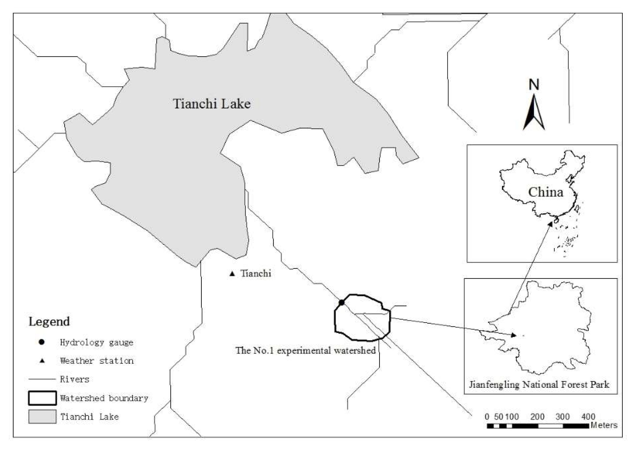
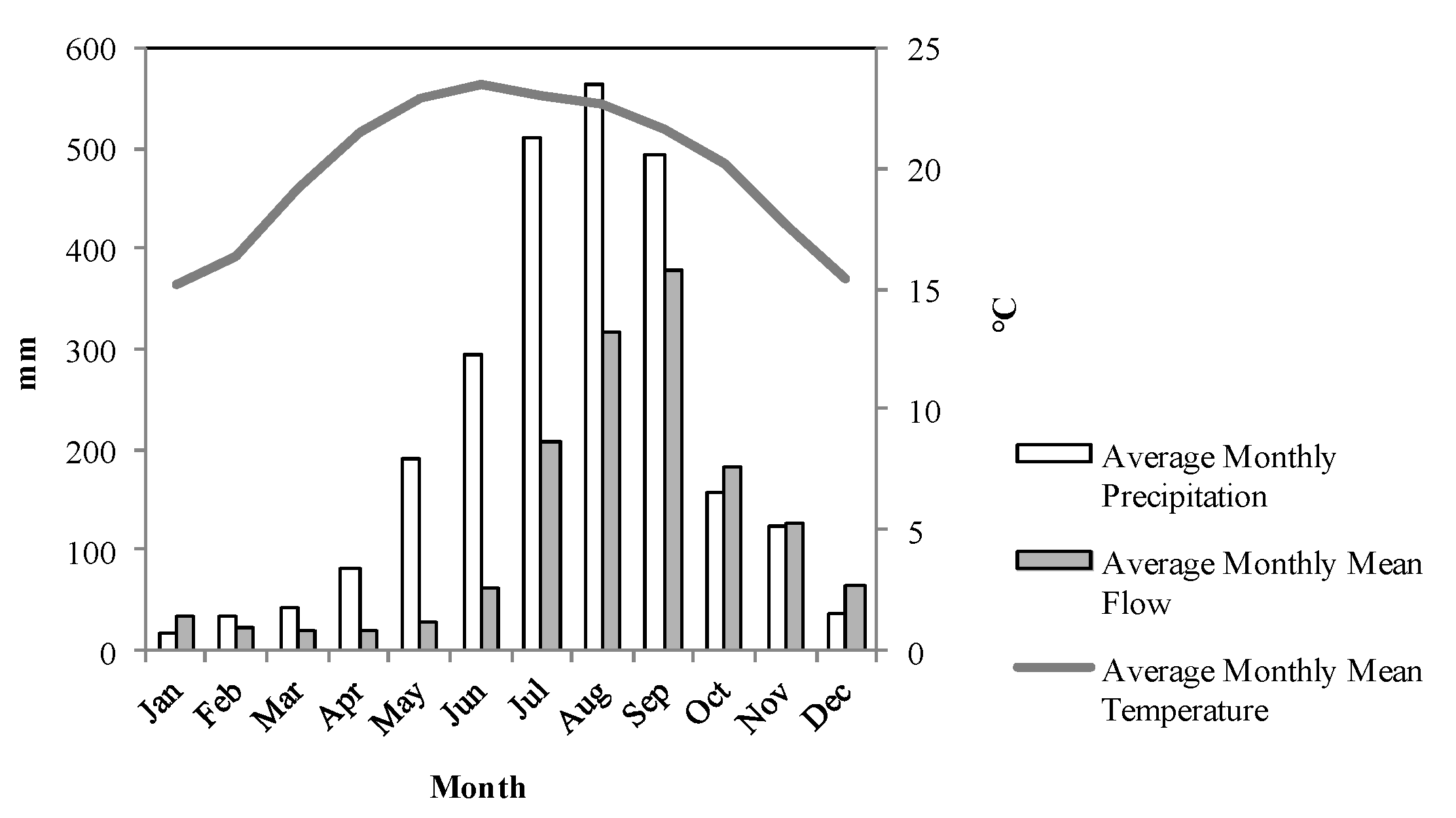
2.1. Study Watersheds

This study was conducted in the No.1 experimental watershed located within the Jianfengling National Forest Park (452.67 km2, latitude: 18°40′ N–18°57′ N, longitude: 108°41′ E–109°12′ E) in the Southwest of Hainan Province, China (Figure 1). The drainage area of the study watershed is 3.01 ha, which is fully covered with secondary tropical forests.
The No.1 experimental watershed lies in the tropical monsoon climate zone with distinct wet and dry seasons [40]. The wet season starts from May to October influenced by frequent cyclones or typhoons with high intensity rainfall [41]. The long-term mean annual precipitation is 2541 mm, of which 87% (2207 mm) falls in the wet season (May to October) and 13% (334 mm) in the dry season (November to April), respectively (Figure 2). The annual mean temperature in this watershed is 19.8 °C, and the maximum mean temperature reaches 23.3 °C (June), while the minimum mean temperature is 14.8 °C (January).
The No.1 experimental watershed was originally covered by natural tropical montane rainforests which were gradually replaced by naturally regenerated secondary tropical rainforests after a clear-cut in 1965 [25]. The commercial harvesting in this experimental watershed stopped in 1993 when the Jianfengling National Forest Park was established. The No.1 experimental watershed as a part of the Jianfengling Park experienced human activities including infrastructure or road construction and recreation since then. The dominant vegetation types include Clerodendrum canescens Wall., Litsea glutinosa (Lour.) C.B.Rob., Cyclobalanopsis kerrii (Craib) Hu, Eurya nitida Korthals, Mallotus paniculatus (Lamb.) Muell. Arg., Trema orientalis (L.) Bl., Microcos paniculata L., Sterculia lanceolata Cav., Litsea monopetala (Roxb.) Pers., Schima superba Gardn. et Champ. and Machilus bombycina King ex Hook.f. [42].
As a tropical coastal watershed, forests in this area are frequently disturbed by typhoons, tropical cyclones and cold waves. Typhoons or tropical cyclones are associated with heavy rain, leading to more than 1000 mm rainfall (one third of annual precipitation) in a few days [43]. During the study period, the most severe typhoon was Lewis occurred in July 1993. It struck the South Hainan Island Coast with its eye passing through the Jianfengling National Forest Park at a wind speed of 41 m/s. The No.1 experimental watershed, located 20 km from the coast, was in close proximity to the path taken by the storm’s eye and received severe damage. The tropical forests in the experimental watershed also suffered from a severe cold wave in December 1999, the strongest cold wave in recent 50 years. The extreme low temperature in the No.1 experimental watershed was 6.4 °C in December 1999 (Figure 3), 5.0 °C below the long-term average extreme low temperature of December (11.7 °C).

2.2. Data

One weir was built in 1989 at the outlet of the No.1 experimental watershed (latitude: 18°44′ N, longitude: 108°51′ E). Hydrological records including flow velocity and water table were continuously measured for a period from 1990 to 2005 in the No.1 experimental watershed [44]. Annual and seasonal (dry and wet season) streamflow, high flows and low flows, and precipitation were calculated based on daily flow records. The hydrological year (November–October) was divided into dry season (November–April) and wet season (May–October).
Climate data were obtained from the Tianchi weather station established near the Tianchi Lake (latitude: 18°43′ N, longitude: 108°52′ E, elevation: 880 m) in 1980, which is 1 km away from the study watershed (latitude: 18°44′ N, longitude: 108°51′ E). Daily temperature data from this station were used in this study. From 1980 to 1988, temperature was measured manually at 2:00 a.m., 8:00 a.m., 14:00 p.m. and 20:00 p.m. every day. The original weather station was then replaced by an automatic one in 1989, and climate data were recorded every 30 min since then. In this study, monthly temperature data from 1990 to 2005 were used.
Forest data used in this study mainly include LAI (Leaf area index, defined as one half of the total green leaf area per unit of horizontal ground surface area) data from the Global Land Surface Satellite Products (GLASS: http://glass-product.bnu.edu.cn/) between 1990 and 2005 [45]. The GLASS LAI product generated from Advanced Very High Resolution Radiometer (AVHRR) reflectance data is available with a temporal resolution of eight days and a spatial resolution of 0.05° from 1982 to 2015 [46,47,48,49]. By use of the GLASS LAI product, we generated two data series of LAI: dry season LAI (mean value of the 1st to 177th day in a year) and wet season LAI (mean value of the 185th to 361th day in a year) from 1990 to 2005 for the No.1 experimental watershed.

2.3. Methods

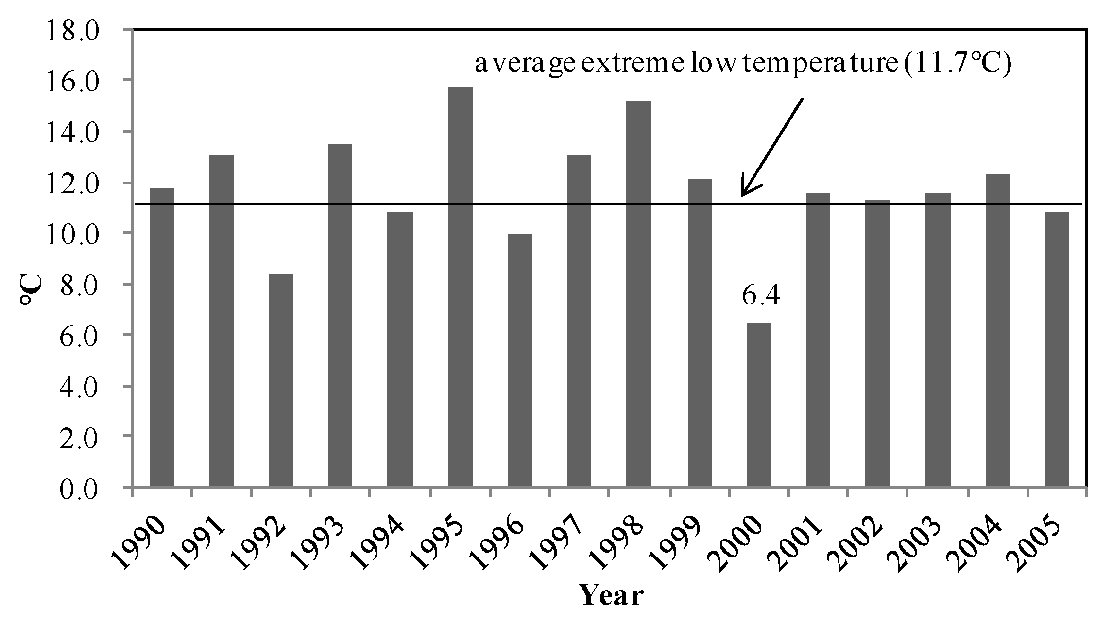
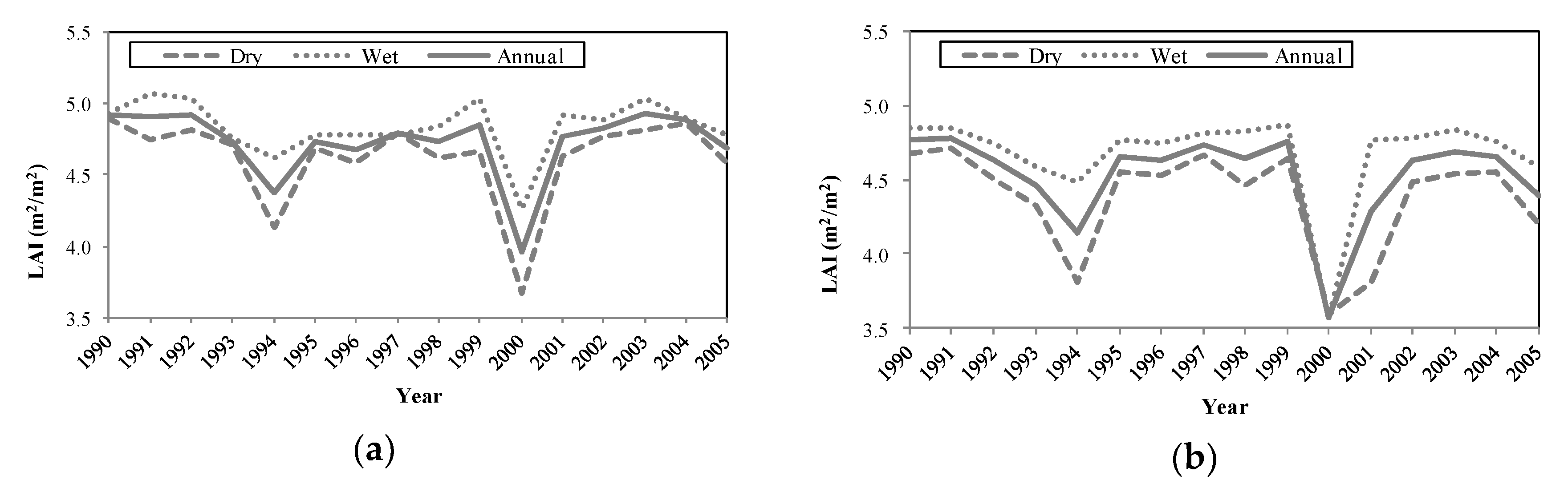
2.3.1. Quantification of Forest Disturbances

Forest disturbances such as logging can be simply described by logged area or forest coverage change since trees are normally removed out of forests. However, such an indicator is inappropriate for extreme weather-induced forest disturbances given that downed, snapped and dead trees remaining in the disturbed forests as well as a large number of trees with loss of branches and leaves. In this study, we selected LAI as an indicator for forest disturbances. LAI is considered to be an important biophysical variable influencing vegetation photosynthesis, transpiration, and land surface energy balance, and thus a good indicator of canopy structure and biomass to reflect vegetation change [38,39,50]. Figure 4 shows annual and seasonal LAI from 1990 to 2005 in the No.1 experimental watershed. The annual LAI varied between 3.965 m2/m2 (2000) and 4.928 m2/m2 (2003), with an average of 4.733 m2/m2.

2.3.2. Trend Analysis

Trend analysis was used in this study to detect whether the climate, hydrological and forest disturbance data have statistical significant upward or downward trends on multiple temporal scales (annual, dry season, wet season) [51,52]. Non-parametric tests, Kendall tau and Spearman rho tests were widely used for trend detection in climate and hydrology due to their fewer assumptions and the ability to eliminate the influences of outliers. For example, Kendall tau and Spearman rho tests are available for both normal and non-normal distribution data series [52].

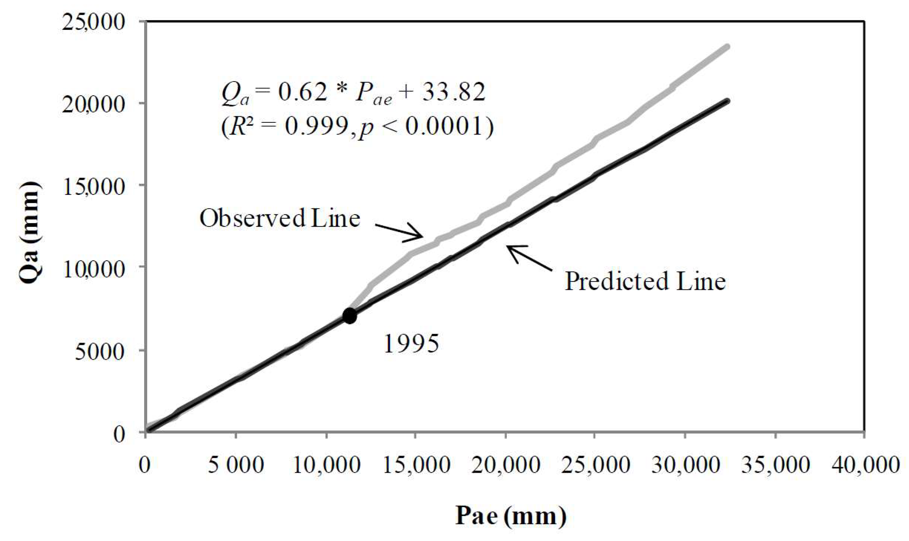
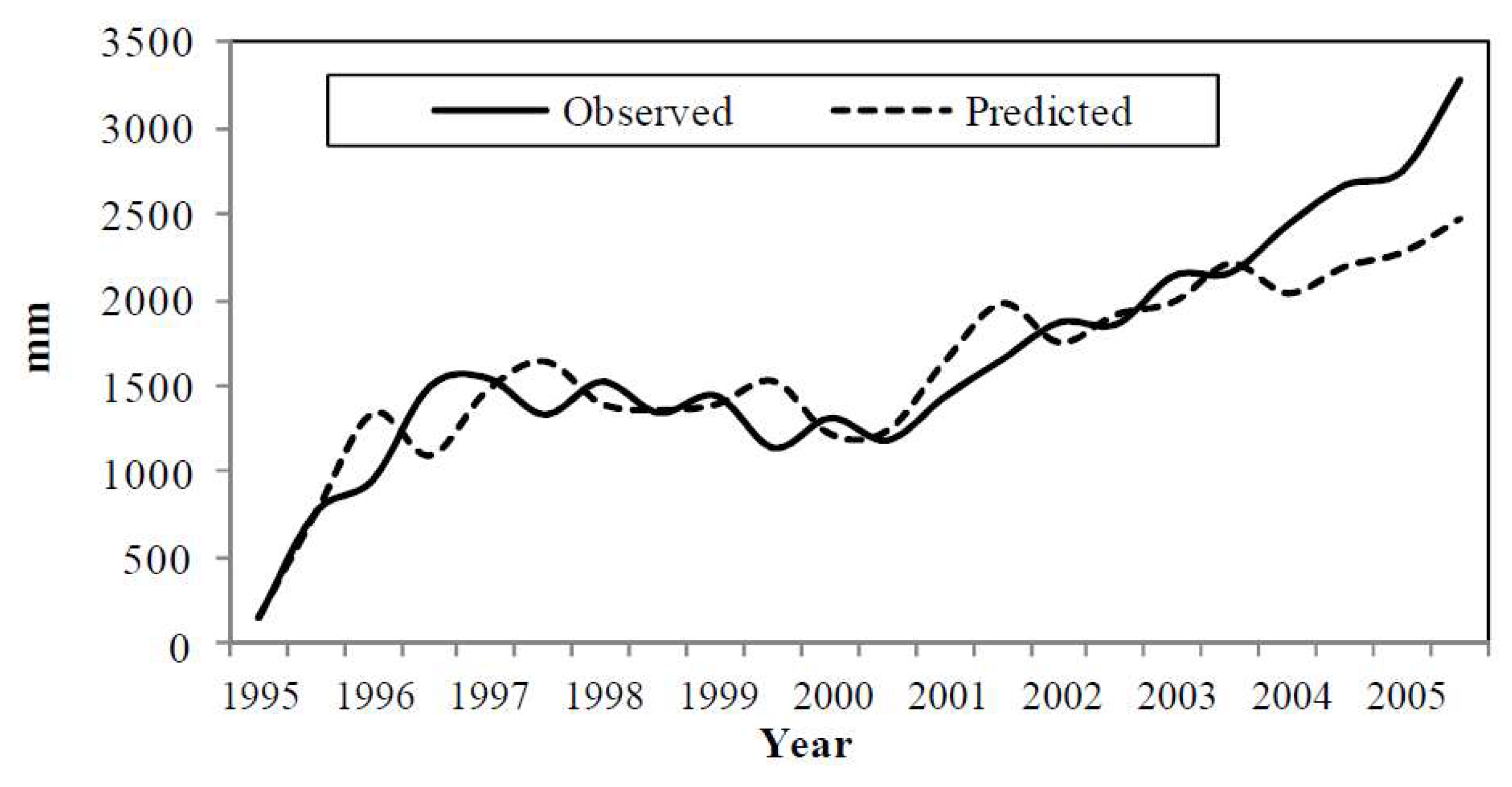
2.3.3. Quantifying the Effects of Climate Variability, Forest Disturbances and Other Factors on Streamflow

The No.1 experimental watershed was perennially affected by extreme weather events and other factors such as human activities. An improved single watershed approach combining the modified double mass curve (MDMC) and time series ARIMAX model was applied to quantify the annual/seasonal streamflow responses to climate variability, forest disturbances and other factors [53].
Wei and Zhang (2010) developed the MDMC to exclude the influence of climate variability on streamflow, which has been successfully applied in many watersheds in Canada and China [22,54,55,56,57]. The MDMC was designed for a single watershed study with fewer data requirements in comparison with the traditional DMC used in the paired watershed studies. In a MDMC, accumulated annual/seasonal effective precipitation was plotted versus accumulated annual/seasonal streamflow, where annual/seasonal effective precipitation (Pe) was the difference between annual/seasonal precipitation (P) and annual/seasonal evapotranspiration (E). Since the effective precipitation indicates available water for streamflow generation, a consistent relationship between streamflow and effective precipitation can be observed in a watershed during a period with limited disturbances. Thus the MDMC is normally a straight line if the effect of non-climate factors (e.g., forest disturbances induced by extreme weather events and other factors) on streamflow is insignificant. In other words, streamflow variation is only determined by climate variability during undisturbed or less disturbed period. Once non-climatic factors such as forest disturbances and human activities produce noticeable impact on streamflow, a breakpoint in the modified double mass curve can be found [22]. Statistical tests, including ARIMA (Autoregressive Integrate Moving Average) Intervention and non-parametric tests (Wilcoxon test and Sign test) were applied to confirm the statistical significance of the breakpoint [58,59]. The period before the breakpoint is defined as the reference period (a period without significant hydrological alteration) when streamflow variation has a consistent linear relation with climate variability. And the period after the breakpoint is named as the disturbed period, a period with significant hydrological alteration. Then, the predicted accumulated seasonal streamflow were estimated by a linear regression model established by observed accumulated seasonal streamflow and accumulated seasonal effective precipitation during the reference period. In this way, the difference between the observed line and predicted line after the breakpoint (disturbed period) can be attributed to accumulated streamflow variation attributed to non-climate factors (∆Qanc), and the effect of climate variability on accumulated streamflow (∆Qac) can be estimated accordingly (Equations (1) and (2)).
Δ Q a n c = Δ Q a Δ Q a 0
Δ Q a n = Δ Q a Δ Q a n c
where Qa and Qa0 are observed accumulated seasonal streamflow, and predicted accumulated seasonal streamflow by the linear regression model after breakpoint, respectively; ∆Qanc stands for accumulated seasonal streamflow variation attributed to non-climate factors; ∆Qac and ∆Qa represent accumulated seasonal streamflow variation attributed to climate variability and streamflow variation, respectively.
We then applied the Multivariate ARIMA (ARIMAX) model to quantify streamflow responses to extreme weather-induced forest disturbances by establishing a quantitative relationship between accumulated seasonal streamflow variation attributed to non-climatic factors (∆Qanc) and seasonal ∆LAIa (accumulated seasonal LAI variation) during the disturbed period. The ARIMAX model is a typical ARIMA model with one or multiple external variables to improve the accuracy of simulation [60], which was widely used in analyzing auto-correlated data series [61]. This method was successfully applied to identify streamflow variation attributed to vegetation change and other factors from non-climate factor in a comparative study in China [53]. An ARIMAX model fitting ∆Qanc with accumulated seasonal LAI variation (∆LAIa) as regressor during the disturbed period was established using SAS version 9.4 (SAS Institute, Inc., Cary, NC, USA). If all parameters in the established ARIMAX model were significant, we can obtain the predicted accumulated streamflow variation attributed to seasonal non-climatic factors (∆Qanc0) from the selected ARIMAX model. The differences between ∆Qanc and ∆Qanc0 (∆Qad) can be viewed as accumulated seasonal streamflow variation attributed to other factors and statistical errors (Equation (3)). Here, the 95% confidence interval (CI) of ∆Qd (seasonal differences of observed and predicted values in the selected ARIMAX model) was used to represent the margins of statistical errors (∆Qse) (Equation (4)). If data points are located within 95% CI, ∆Qd only indicates statistical errors and other factors yield an insignificant effect on seasonal streamflow. However, for those data points distributed beyond 95% CI, other factors produced significant impact on seasonal streamflow. In this way, seasonal streamflow variation attributed to other factors (∆Qo) can be estimated and the response due to extreme weather-induced forest disturbances (∆Qf) can be computed accordingly (Equation (5)).
Δ Q a d = Δ Q a n c Δ Q a n c 0
Δ Q o = Δ Q d Δ Q s e
Δ Q f = Δ Q n c Δ Q o
where ∆Qanc, and ∆Qanc0 stand for observed and predicted accumulated seasonal streamflow variation attributed to non-climatic factors, ∆Qad is accumulated seasonal streamflow variation from others. ∆Qd, ∆Qf and ∆Qo represent seasonal streamflow variations attributed to others, forest disturbances and other factors; ∆Qse is statistical errors from the ARIMAX model.

2.3.4. Quantifying the Effect of Forest Disturbances on High Flows and Low Flows

Flow duration curve (FDC), a widely used hydrograph, shows the percentage of time that streamflow equals or exceeds a given amount over a time interval, for example, annually or monthly [6]. Flows at a given percentile (denoted as Qp%) can be derived from FDC. In this study, high flows (Qh) refer to flows equal to or beyond Q5%, and low flows (Ql) are defined as flows equal to or below Q95%, where Q5% and Q95% are flow exceeded at 5% and 95% of the time in a given year. According to definitions above, annual data series of high and low flows were generated.
The paired-year approach was then used to assess the changes of magnitude in high flows and low flows [62]. In the paired-year approach, a reference year (before the breakpoint of MDMC) was paired with a disturbed year (after the breakpoint of MDMC) according to their similarities in annual mean temperature and precipitation, where the effect of climate variability on streamflow can be eliminated [62]. To precisely assess the effect of extreme weather-induced forest disturbances on high flows and low flows, we also consider if extreme weather events happened around selected disturbed years. Based on the criteria above, we identified two pairs in this study (Table 1). Mann–Whitney U test was performed to detect the statistical significance of differences in the medians of high flows/low flows between the reference year and disturbed year for each pair. In this way, the effects of forest disturbances on high flows/low flows were eventually quantified.

3. Results

3.1. Trend Analysis of Hydrological, Climatic and Forest Disturbance Variables

From 1990 to 2005, annual streamflow ranged from 477 mm to 2516 mm, with an average of 1465 mm. Mean annual precipitation reached 2524 mm (1252–3948 mm). Calculated by Thornthwaite method and Zhang’s equation (a modification of Budyko’s evaporation), annual evapotranspiration is much lower than annual streamflow, varied from 432 mm to 570 mm, with an average value of 503 mm, suggesting the No.1 experimental watershed a high water yield ecosystem. According to the trend analysis (Table 2), a significant downward trend (α = 0.05) was detected in wet season evapotranspiration, whilst significant upward tendency in temperature (annual, dry season and wet season) was identified due to global warming [63,64]. In addition, no significant trend in other variables were found.

3.2. Effects of Forest Disturbances on Annual and Seasonal Streamflow

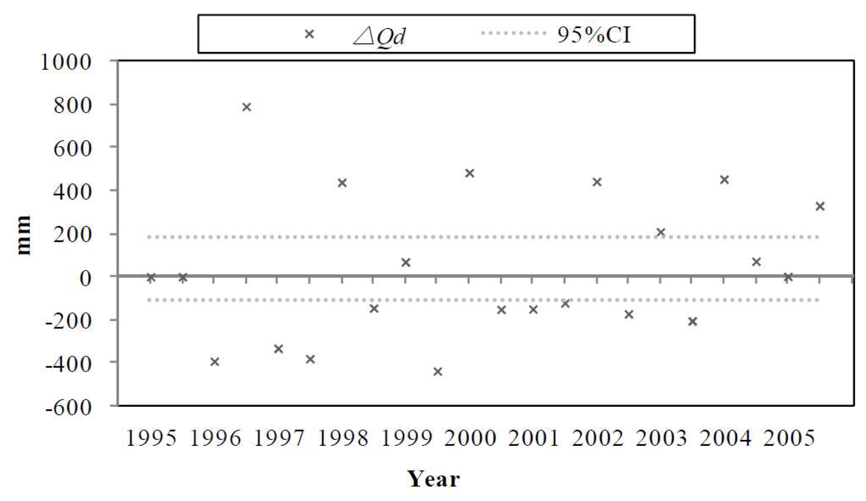
3.2.1. Annual and Seasonal Streamflow Variations Attributed to Non-Climatic Factors

A breakpoint occurred in 1995 was found in modified double mass curve (Figure 5). The ARIMA intervention test of the MDMC slopes and non-parametric tests (Wilcoxon test and Sign test) both confirmed statistical significance of the breakpoint (α = 0.05) (Table 3 and Table 4). As estimated, accumulated seasonal streamflow variation attributed to non-climatic factors were from 145.7 mm to 3270.5 mm while accumulated seasonal streamflow variation attributed to climate variability varied from −210.3 mm to −2468.7 mm during 1995–2005.

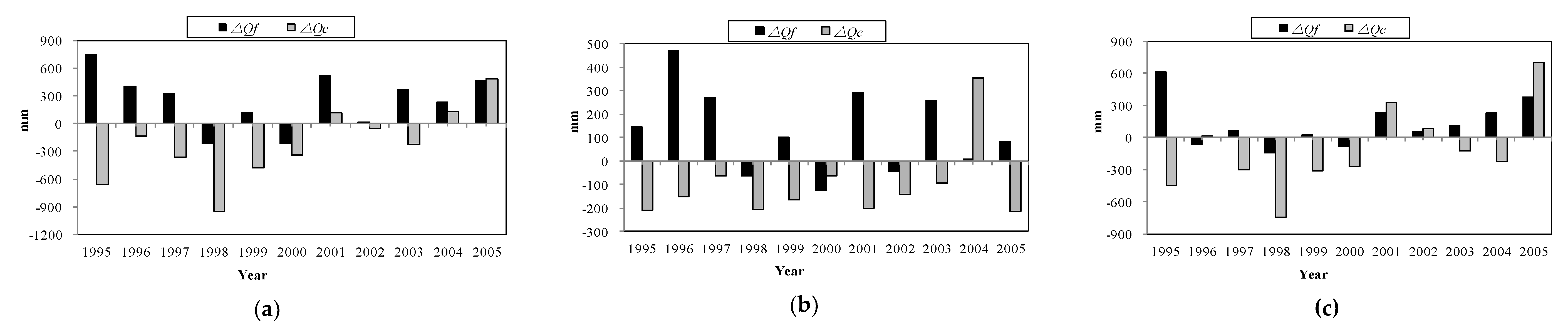
3.2.2. Annual and Seasonal Streamflow Variations Attributed to Forest Disturbances

Table 5 showed the model structure and parameters of the best fitted ARIMAX model. The significant differences between observed accumulated seasonal streamflow variation attributed to non-climatic factors and its predicted values are associated with statistical errors and other factors (Figure 6). As shown in Figure 7, 17 data points falling outside the 95% CI (statistical errors) of predicted seasonal streamflow variation to non-climatic factors were identified as seasonal streamflow. This indicated that seasonal flows in these seasons were significantly affected by other factors and forest disturbances. On the contrary, the remaining five data points (1995 dry season and wet season, 1999 dry season, 2004 wet season and 2005 dry season) fell within the 95% CI, suggesting that streamflow variation attributed to other factors in these seasons is minor.
According to the final analysis, forest disturbances mainly increased annual/dry/wet season streamflow while climate variability decreased annual/dry/wet season streamflow during 1995–2005 (Figure 8). Average annual/dry/wet season streamflow variations attributed to forest disturbances over the disturbed period were 126.7 mm, 127.0 mm, and 126.3 mm, respectively, and the relative contributions of forest disturbances to annual/dry/wet season streamflow were 48.6%, 44.7%, and 50.0%. Average annual/dry/wet season streamflow variations attributed to climate variability from 1995 to 2005 were −112.2 mm, −105.5 mm, and −118.9 mm, respectively, and the relative contributions of climate variability to annual/dry/wet season streamflow were 43.0%, 37.2%, and 47.1%. Other factors were less influential on streamflow in the study watershed. Average annual/dry/wet season streamflow variations attributed to other factors from 1995–2005 were only 22.0 mm, 51.4 mm, and −7.4 mm, respectively and the relative contributions of other factors to annual/dry/wet season streamflow were 8.4%, 18.1%, and 2.9% (Table 6).
From 1995–1999, forest disturbances led to a greater increment of streamflow in dry season while during 2000–2005 wet season streamflow response to forest disturbances was higher. Average dry season streamflow variation attributed to forest disturbances was 184.6 mm and wet season streamflow response was 95.9 mm from 1995–1999 (Table 6). On the contrary, average dry season streamflow variation attributed to forest disturbances was 79.0 mm and wet season streamflow response was up to 151.7 mm from 2000 to 2005. Unlike forest disturbances, climate variability can yield different effects on streamflow in different periods. From 1995–1999, climate variability produced negative effects on streamflow and average annual/dry/wet season streamflow variations attributed to climate variability were −259.8 mm, −159.1 mm, and −360.4 mm, respectively. However, climate variability had positive influence on annual and wet season streamflow during 2000–2005. Average annual and wet season streamflow variations attributed to climate variability were 10.8 mm and 82.4 mm then (Table 6).

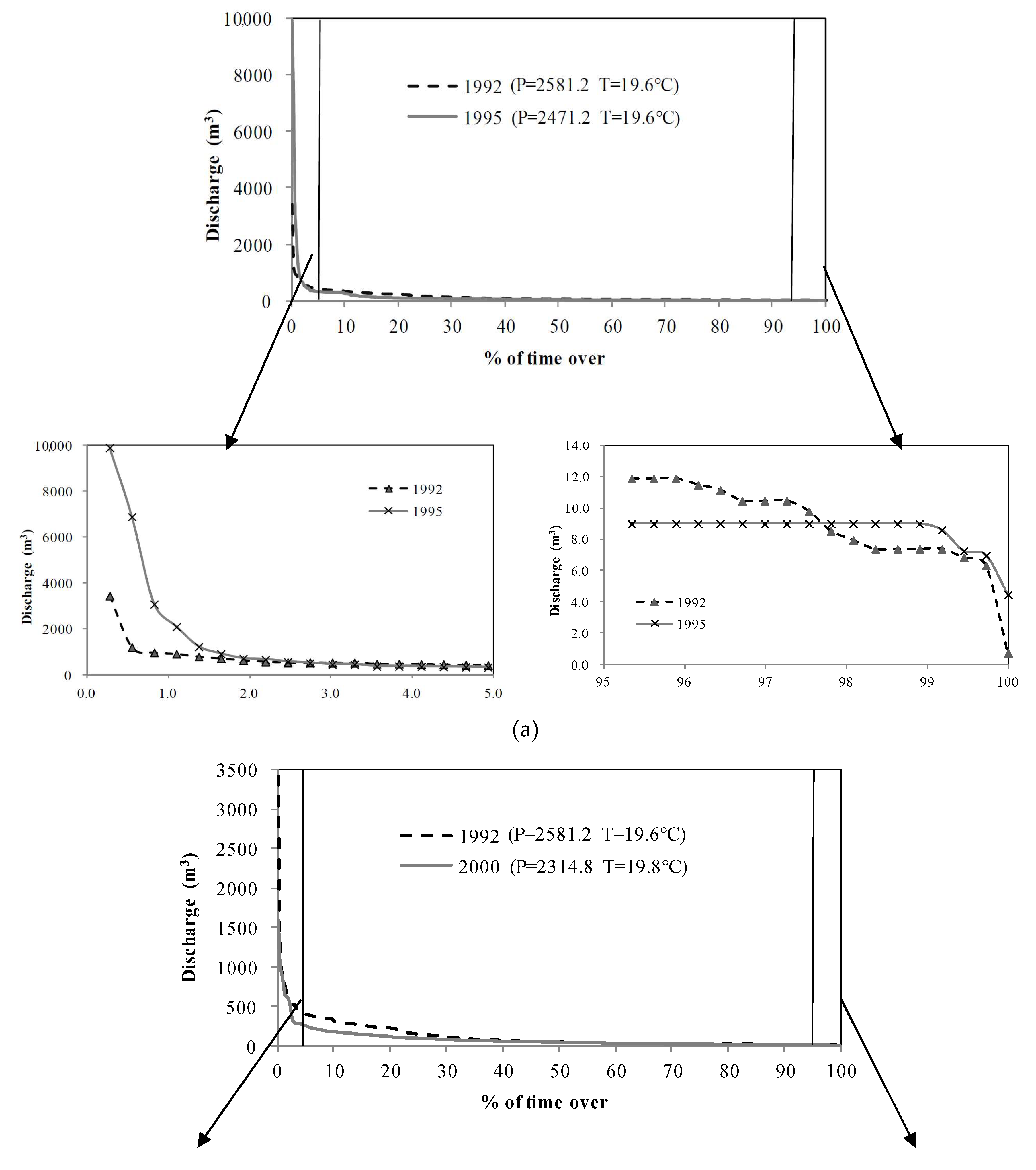
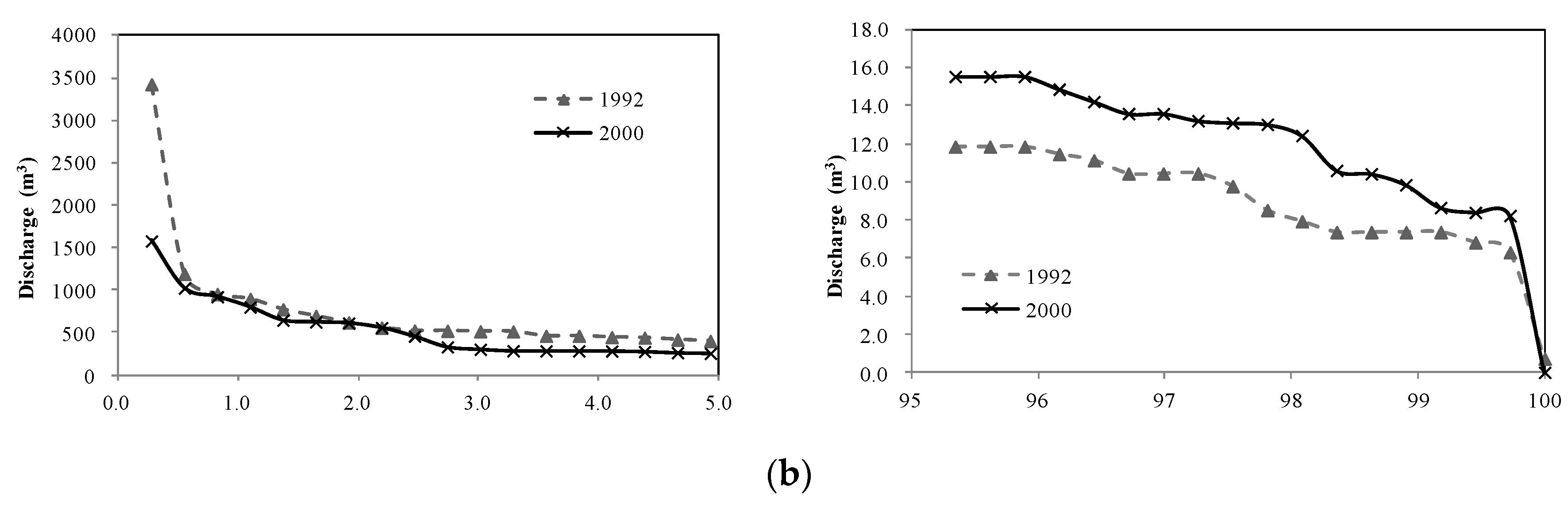
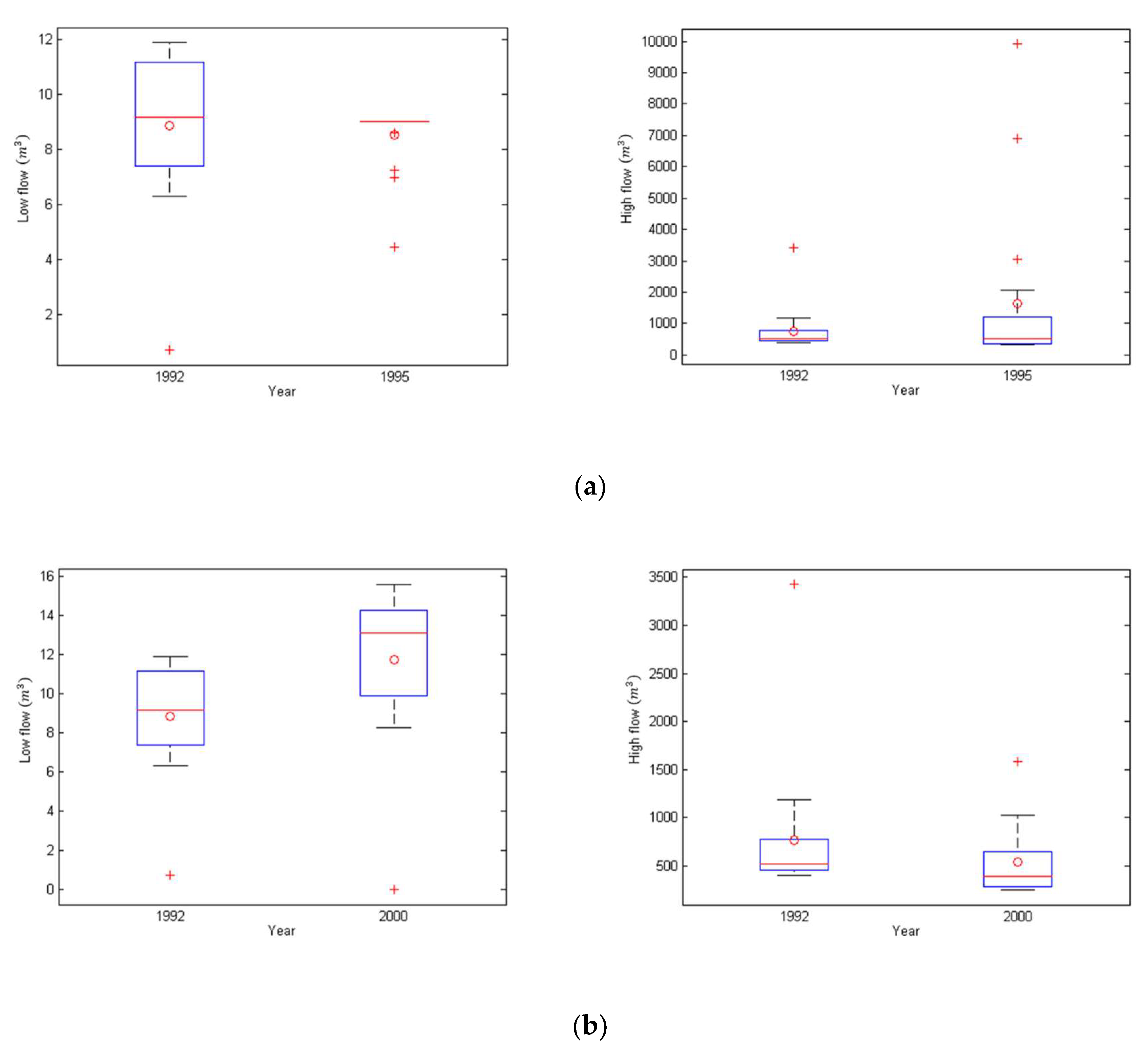
3.3. Effects of Forest Disturbances on High Flows and Low Flows

Figure 9 shows flow duration curves (FDCs) for the two paired years. As suggested by Box-plot and Mann–Whitney U test (Figure 10 and Table 7), for the # 2 pair the median of low flows in 2000 (the disturbed year) was significantly higher than that in 1992 (the reference year) at α = 0.05 while insignificant differences in the median of high flows were detected between them. The median of low flows in the reference year (1992) was 9.8 m3/s, ranging from 0.7 m3/s to 11.9 m3/s, while in the year 2000, the median of low flows reached 13.1 m3/s (from 0.0 m3/s to 15.6 m3/s). The differences in the medians of high flows or low flows between the disturbed year 1995 and the reference year 1992 were statistically insignificant at α = 0.05.

4. Discussion

4.1. Forest Changes Due to Typhoon and Cold Wave

Sharp reductions of LAI saw in 1994 and 2000 in the No.1 experimental watershed (Figure 4). The sharp decline of LAI in 1994 was associated with the typhoon Lewis which happened in July 1993. After the pass of the storm, mean LAI during the dry season of 1994 (November 1993 to April 1994) was greatly decreased by 12.4% as compared to the mean for dry season of 1993. Storm, typhoon or hurricane associated damage on forests normally include uprooting, trunk breakage, branch snapping and defoliation, resulting in more forest gaps, lower canopy density, and even tree mortality and eventually lower LAI [27,30,31,65,66]. For example, in the 22-year-old community-managed secondary forest at Manobo near Tacloban on Leyte Island in the central Philippines, Zhang et al. (2015) found LAI dropped by 27.5% after Typhoon Haiyan on 8 November 2013 [67]. Similarly, the subtropical forests of Puerto Rico hit by Hurricane Hugo in September 1989 were found with about a quarter of the trees destroyed, and 9% tree mortality [68].
However, the impact of cold wave on forests can be more pronounced than typhoon in the study watershed. According to our analysis, mean LAI during the dry season of 2000 (November 1999 to April 2000) and the wet season of 2000 (May 2000 to October 2000) greatly decreased by 21.3% and 15.5% as compared to their means in 1999. Given the absence of large typhoons from 1997 to 1999, the sharp decline in LAI was due to the cold wave in December 1999, the strongest one in recent 50 years. This cold wave with long-lasting extreme low temperature below the long-term average inhibited the growth of vegetation and led to high mortality of trees, resulting in a sharp drop in LAI. As documented by many studies, the growth of tropical vegetation is very sensitive to winter temperature [69,70,71,72]. Extreme low temperature can slow down photosynthesis, transpiration, and translocation of the starch of tropical trees, leading to lower biomass accumulation [73,74,75]. A similar study by Hilliard and West (1970) also found the growth of Digitaria decumbens (Gramineae) (a tropical plant) was severely reduced when the temperature is 10 °C or below. Therefore, according to the above analysis, typhoon disturbances and cold waves yielded significant negative impact on forest growth [76].

4.2. Annual/Seasonal Streamflow Response to Forest Disturbances

According to the modified double mass curve and quantification analysis, forest disturbances produced significant positive effects on dry season, wet season, and annual streamflow in the No.1 experimental watershed from 1995 to 2005. Dry season, wet season, and annual streamflow were increased by 43.8% (127.0 mm), 10.8% (126.3 mm), and 17.2% (126.7 mm), respectively as a result of LAI reduction ascribed to forest disturbances including cold wave and typhoon. This is in accordance with some findings from tropical watershed studies that deforestation (e.g., harvesting, urbanization, and wildfire) can increase streamflow. For example, Costa et al. (2003) denoted that a 19% forest loss produced a significant increase in annual streamflow in Tocaintins River watershed in Southeast Asia [77]. On one hand, forest disturbance induced by typhoon, cold wave, and logging can lead to reduced canopy interception of rainfall and less transpiration, and consequently more water available for streamflow generation. On the other hand, these forest disturbances can lead to a decline in growth rate of tree due to less active photosynthesis, lower transpiration rate and less evaporation, and eventually with less water consumption and more streamflow [65,78].
It is well known that climatic conditions are crucial for hydrological processes in forest watersheds [59,79]. Our analysis showed that during the dry period (1995–1999), annual streamflow is more sensitive to forest disturbances than during the wet period (2000–2005). The average increment in annual streamflow was 140.3 mm (19.2%) from 1995–1999 (P = 2111.9 mm) while the increment was only 115.3 mm (15.8%) from 2000–2005 (P = 2814.1 mm) in this watershed. These results are similar to a global review, which indicates that the sensitivity of annual streamflow to forest change is closely related to dryness index [80]. In drier areas or drier years, forest change can produce a noticeable effect on streamflow. In dry season, water availability is the limiting factor for vegetation growth, while energy input in terms of temperature and radiation become the dominant factor given that saturated soils are prevalent in wet season [80]. Consequently, forest change tends to generate more pronounced hydrological impacts in dry season or drier years.

4.3. The Effect of Forest Disturbances on High Flow and Low Flow

The impact of typhoon-induced forest change on hydrological extremes tended to be less than that of cold wave-induced forest change. The differences in both high flows and low flows between 1995 (the year after the typhoon Liews) and 1992 (the reference year) were insignificant. Similarly, the response of high flows to cold wave-induced forest change in 2000 was insignificant. High flows in the study watershed often occur in the typhoon season, which are mainly caused by typhoon related heavy rain or storms. The effect of tropical forests in the generation of high flows is believed to be less than climate such as storms or typhoon associated heavy rain [81]. However, the magnitude of low flows was significantly increased by cold wave-induced forest disturbances. As mentioned before, the cold wave with long-lasting extreme low temperature can lead to a slow-down of photosynthesis and transpiration of tropical trees and losses of leaves, resulting in less water consumption and more water available for streamflow generation especially during the low flow season. In addition, this study watershed is classified as an energy-limited watershed (Budyko dryness index (DI) < 0.76), where forest growth tends to be less dependent on water availability but responds more strongly to temperature [59,79,80,82,83]. Therefore, lower temperature can lead to more pronounced hydrological responses in the study watershed.

4.4. Implications for Watershed Management

In forested watersheds, forest disturbances and climate variability are two major drivers for hydrological changes. Understanding their interactive, dynamic effects is important for sustainable water supply and flood control. Forest disturbances and climate variability can influence streamflow in the same or opposite (offsetting) directions with different strengths.
According to the analysis in the No.1 experimental watershed, forest disturbances and climate variability produced opposite impacts on dry season, wet season and annual streamflow during 1995 and 1999. During that dry period (1995–1999), forest disturbances increased dry/wet season and annual streamflow by 184.6 mm, 95.9 mm and 140.3 mm, respectively, while climate variability decreased dry/wet season and annual flow by 159.1 mm, 360.4 mm and 259.8 mm, respectively. The counteracting or cancelling effects of forest disturbances and climate variability eventually reduced annual variations of streamflow over the period of 1995 to 1999 in the study watershed, which can benefit water resources management by providing a stable water supply especially in dry years [55,57,84]. However, from 2000 to 2005 both forest disturbances and climate variability produced positive effects on streamflow. During the wet period (2000–2005), forest disturbances averagely yielded 151.7 mm and 115.3 mm increments in wet season and annual streamflow, respectively, and climate variability also contributed to 82.4 mm and 10.8 mm increments in the wet season and annual streamflow, respectively. The additive effects of forest disturbances and climate variability on wet season streamflow can lead to potential risks of larger floods, and greater challenges for flood control and eventually threatening downstream public safety [22]. As forests and climate continue to change in the future, their combined effects (offsetting or additive) on streamflow will have significant implications for watershed management and public safety.
In addition to the impact directions of climate variability and forest disturbances, their strength or relative contributions to streamflow variations are also important and meaningful. Over the whole disturbed period, forest disturbances accounted for a 48.6% change in annual streamflow while the relative contribution of climate variability is 43.0%, further suggesting that both forest disturbances and climate variability are important drivers for streamflow variations and forest disturbances are relatively more influential [55,85]. Contrarily, there are studies that found climate variability produced greater impact on streamflow than forest disturbances. In the Heihe River watershed of China, climate variability accounted for up to 95.8% of changes in streamflow while forest disturbance only explained 9.6% [86]. Another study in the central interior of British Columbia, Canada also found relative contributions from climate variability on annual streamflow (55%) was greater than forest harvesting (45%) in the Willow River Watershed [54]. These differences indicate the impact strength of different forests on water cycle. Tropical forests with higher evapotransipration may have greater impact on water cycle than temperate forests.
The relative contributions of forest disturbances and climate variability to streamflow variations may change over time especially in the context of global warming. During 1995–1999, climate variability was more influential on streamflow than forest disturbances. The relative contributions of climate variability on annual streamflow variation reaches 60.8% while the contribution from forest disturbances after the typhoon Lewis (1994) was only 32.8%. However, after the strong cold wave in December 1999, forest disturbances became a dominating factor on streamflow variation during 2000–2005. The relative contributions of forest disturbances on annual streamflow variation was 61.0%, while the contributions from climate variability were only 5.7%.
Forests play an important role in water balance in tropical regions to keep sustainable water supply. As is known, tropical forest ecosystem is very complex. Once the “sponge effect” of tropical forests is damaged, it will take a long time (more than 30 years) to reach a full hydrological recovery [5]. Moreover, Hainan Island is surrounded by ocean, frequently suffered from extreme weather events due to the monsoon from the Indian Ocean and Pacific Ocean. At the same time, tropical coastal ecosystems can experience frequent extreme weather events caused by El Niño southern oscillation [87]. As suggested by this study, forest disturbances especially cold wave-induced forest changes also generated greater influence on low flows, reducing the risks of drought. In addition, the offsetting effects of forest disturbances and climate variability on dry season streamflow can benefit water resources management especially in dry years, while the additive effects of forest disturbances and climate variability on wet season streamflow will increase the risk of floods. Obviously, the frequency of extreme weather events are increasing with climate change, which are expected to yield more significant impact on forest ecosystem and hydrological cycle even in the coastal headwaters such as the No.1 experimental watershed.

4.5. Uncertainties Assciated with LAI Data

The LAI data we used is GLASS product with a spatial resolution of 0.05°, but the drainage area of the study watershed is only 3.01 ha. The mismatched spatial resolution may lead to a concern about the representation of forest conditions by the LAI data used in the study watershed. In fact, LAI was used to indicate the average status of vegetation at a watershed scale rather than showing the spatial patterns or variations of disturbed patches in the forests. Since the study watershed and Jianfengling National Forest Park have similarities in topography, climate and forest conditions including age, species and structures, the changes in the average status of vegetation can be similar after typhoon or cold wave. In order to validate the LAI data in the study watershed, we also collected the LAI data of the Jianfengling National Forest Park (452.67 km²) and compared the changes in the LAI of study watershed and the Jianfengling National Forest Park from 1990–2005 (Figure 4b). We found the change patterns in the dry, wet and annual LAI of the study watershed were in accordance with those in the Jianfengling National Forest Park. The linear correlation and Kendall tau correlation analysis confirmed that dry, wet and annual LAI of the study watershed were significantly correlated with those in the Jianfengling National Forest Park (Table 8). In addition, we actually used ∆LAIa that indicated temporal variations in LAI as the regressor for ARIMAX modelling. Thus, we believe the bias associated with the use of GLASS product in the study watershed can be minor. However, ground measurements of LAI in the study watershed are suggested to perform in the future for a better validation of remote-sensed vegetation data.

5. Conclusions

Forest disturbances were more influential on streamflow variation than climate variability in the No.1 experimental watershed from 1995 to 2005. Forest disturbances generally produced significant positive effects on dry season, wet season, and annual streamflow over the study period, while climate variability yielded negative or positive effects on streamflow in different periods. In addition, forest disturbances especially cold wave-induced forest change also generated greater influence on low flows, reducing the risks of drought. In addition, the offsetting effects of forest disturbances and climate variability on streamflow, in particular, on dry season streamflow can benefit water resources management, while the additive effects of forest disturbances and climate variability on wet season streamflow will lead to potential risks of larger floods and greater challenges for flood control. These findings are of great importance for water resource and forest management in the tropical forested watersheds in the context of global warming.

Author Contributions

Data interpretation, T.Y.; Data analysis, Y.H.; Manuscript drafting, Y.H. and M.Z.; Research design, M.Z.; Manuscript revision, S.L., P.S., Y.L., L.Y., Q.L. and X.W.

Funding

This research was supported by National Program on Key Research and Development Project of China (No. 2017YFC0505006), Open Funds of Key Laboratory for Groundwater and Ecology in Arid and Semi-Arid Areas, CGS (No.KLGEAS201801) and China National Science Foundation (No.31770759).

Conflicts of Interest

The authors declare no conflict of interest.

References

  1. Bosch, J.M.; Hewlett, J.D. A review of catchment experiments to determine the effect of vegetation changes on water yield and evapotranspiration. J. Hydrol. 1982, 55, 3–23. [Google Scholar] [CrossRef]
  2. Sahin, V.; Hall, M.J. The effects of afforestation and deforestation on water yields. J. Hydrol. 1996, 178, 293–309. [Google Scholar] [CrossRef] [Green Version]
  3. Stednick, J.D. Monitoring the effects of timber harvest on annual water yield. J. Hydrol. 1996, 176, 79–95. [Google Scholar] [CrossRef]
  4. Andréassian, V. Waters and forests: From historical controversy to scientific debate. J. Hydrol. 2004, 291, 1–27. [Google Scholar] [CrossRef]
  5. Bruijnzeel, L.A. Hydrological functions of tropical forests: Not seeing the soil for the trees? Agric. Ecosyst. Environ. 2004, 104, 185–228. [Google Scholar] [CrossRef]
  6. Brown, A.E.; Zhang, L.; Mcmahon, T.A.; Western, A.W.; Vertessy, R.A. A review of paired catchment studies for determining changes in water yield resulting from alterations in vegetation. J. Hydrol. 2005, 310, 28–61. [Google Scholar] [CrossRef]
  7. Moore, R.D.; Wondzell, S.M. Physical hydrology and the effects of forest harvesting in the Pacific Northwest: A review. JAWRA J. Am. Water Resour. Assoc. 2010, 41, 763–784. [Google Scholar] [CrossRef]
  8. Van Dijk, A.I.J.M.; A-Arancibia, J.L.P.; Bruijnzeel, L.A. Land cover and water yield: Inference problems when comparing catchments with mixed land cover. Hydrol. Earth Syst. Sci. 2012, 16, 3461–3473. [Google Scholar] [CrossRef] [Green Version]
  9. Floren, A.; Linsenmair, K.E. The influence of anthropogenic disturbances on the structure of arboreal arthropod communities. Plant Ecol. 2001, 153, 153–167. [Google Scholar] [CrossRef]
  10. Hong, N.M.; Chu, H.J.; Lin, Y.P.; Deng, D.P. Effects of land cover changes induced by large physical disturbances on hydrological responses in Central Taiwan. Environ. Monit. Assess. 2010, 166, 503–520. [Google Scholar] [CrossRef] [PubMed]
  11. Liu, M.; Tian, H.; Lu, C.; Xu, X.; Chen, G.; Ren, W. Effects of multiple environment stresses on evapotranspiration and runoff over Eastern China. J. Hydrol. 2012, 426, 39–54. [Google Scholar] [CrossRef]
  12. Hallema, D.W.; Sun, G.; Caldwell, P.V.; Norman, S.P.; Cohen, E.C.; Liu, Y.; Bladon, K.D.; Mcnulty, S.G. Burned forests impact water supplies. Nat. Commun. 2018, 9, 1307. [Google Scholar] [CrossRef] [PubMed] [Green Version]
  13. Schindler, D.W. The cumulative effects of climate warming and other human stresses on Canadian freshwaters in the new millennium. Can. J. Fish. Aquat. Sci. 2001, 58, 18–29. [Google Scholar] [CrossRef]
  14. Stinson, G. Mountain pine beetle and forest carbon feedback to climate change. Nature 2008, 452, 987–990. [Google Scholar]
  15. Anderegg, W.R.L.; Kane, J.M.; Anderegg, L.D.L. Consequences of widespread tree mortality triggered by drought and temperature stress. Nat. Clim. Chang. 2013, 3, 30–36. [Google Scholar] [CrossRef]
  16. Pretzsch, H.; Biber, P.; Schütze, G.; Uhl, E.; Rötzer, T. Forest stand growth dynamics in Central Europe have accelerated since 1870. Nat. Commun. 2011, 5, 4967. [Google Scholar] [CrossRef] [PubMed]
  17. Jolly, W.M.; Cochrane, M.A.; Freeborn, P.H.; Holden, Z.A.; Brown, T.J.; Williamson, G.J.; Bowman, D.M.J.S. Climate-induced variations in global wildfire danger from 1979 to 2013. Nat. Commun. 2015, 6, 7537. [Google Scholar] [CrossRef] [PubMed] [Green Version]
  18. Bebi, P.; Seidl, R.; Motta, R.; Fuhr, M.; Firm, D.; Krumm, F.; Conedera, M.; Ginzler, C.; Wohlgemuth, T.; Kulakowski, D. Changes of forest cover and disturbance regimes in the mountain forests of the alps. For. Ecol. Manag. 2016, 388, 43–56. [Google Scholar] [CrossRef] [PubMed]
  19. Woods, A. Is the health of British Columbia’s forests being influenced by climate change? If so, was this predictable? Can. J. Plant Pathol. 2011, 33, 117–126. [Google Scholar] [CrossRef]
  20. Stahl, K.; Moore, R.; Mckendry, I. Climatology of winter cold spells in relation to mountain pine beetle mortality in British Columbia, Canada. Clim. Res. 2006, 32, 13–23. [Google Scholar] [CrossRef] [Green Version]
  21. Logan, J.A.; Powell, J.A. Ghost forest, global warming, and the mountain pine beetle (Coleoptera: Scolytidae). Am. Entomol. 2001, 47, 160–172. [Google Scholar] [CrossRef]
  22. Zhang, M.; Wei, X. The effects of cumulative forest disturbance on streamflow in a large watershed in the central interior of British Bolumbia, Canada. Hydrol. Earth Syst. Sci. 2012, 16, 2021–2034. [Google Scholar] [CrossRef] [Green Version]
  23. Lugo, A.E. Visible and invisible effects of hurricanes on forest ecosystems: An international review. Austral Ecol. 2010, 33, 368–398. [Google Scholar] [CrossRef]
  24. Rodriguez-Iturbe, I. Ecohydrology: A hydrologic perspective of climate-soil-vegetation dynamies. Water Resour. Res. 2000, 36, 3–9. [Google Scholar] [CrossRef] [Green Version]
  25. Schlyter, P.; Stjernquist, I.; Bärring, L.; Jönsson, A.; Nilsson, C. Assessment of the impacts of climate change and weather extremes on boreal forests in Northern Europe, focusing on Norway spruce. Clim. Res. 2006, 31, 75–84. [Google Scholar] [CrossRef]
  26. Bernard, B.; Vincent, K.; Frank, M.; Anthony, E. Comparison of extreme weather events and streamflow from drought indices and a hydrological model in river Malaba, Eastern Uganda. Int. J. Environ. Stud. 2013, 70, 940–951. [Google Scholar] [CrossRef]
  27. Jayakaran, A.D.; Williams, T.M.; Ssegane, H.; Amatya, D.M.; Song, B.; Trettin, C.C. Hurricane impacts on a pair of coastal forested watersheds: Implications of selective hurricane damage to forest structure and streamflow dynamics. Hydrol. Earth Syst. Sci. Discuss. 2013, 10, 11519–11557. [Google Scholar] [CrossRef]
  28. Clarke, P.J.; Knox, K.J.E.; Bradstock, R.A.; Munoz-Robles, C.; Kumar, L. Vegetation, terrain and fire history shape the impact of extreme weather on fire severity and ecosystem response. J. Veg. Sci. 2014, 25, 1033–1044. [Google Scholar] [CrossRef]
  29. Harder, P.; Pomeroy, J.W.; Westbrook, C.J. Hydrological resilience of a Canadian rockies headwaters basin subject to changing climate, extreme weather, and forest management. Hydrol. Process. 2015, 29, 3905–3924. [Google Scholar] [CrossRef]
  30. Hogan, J.A.; Zimmerman, J.K.; Thompson, J.; Nytch, C.J.; Uriarte, M. The interaction of land-use legacies and hurricane disturbance in subtropical wet forest: Twenty-one years of change. Ecosphere 2016, 7. [Google Scholar] [CrossRef]
  31. Yang, H.; Liu, S.; Cao, K.; Wang, J.; Li, Y.; Xu, H. Characteristics of typhoon disturbed gaps in an old-growth tropical montane rainforest in Hainan Island, China. J. For. Res. 2017, 28, 1231–1239. [Google Scholar] [CrossRef]
  32. Stanturf, J.A.; Goodrick, S.L.; Outcalt, K.W. Disturbance and coastal forests: A strategic approach to forest management in hurricane impact zones. For. Ecol. Manag. 2007, 250, 119–135. [Google Scholar] [CrossRef]
  33. Kupfer, J.A.; Myers, A.T.; Mclane, S.E.; Melton, G.N. Patterns of forest damage in a Southern Mississippi landscape caused by hurricane Katrina. Ecosystems 2008, 11, 45–60. [Google Scholar] [CrossRef]
  34. Amatya, D.M.; Harrison, C.A.; Trettin, C.C. Water quality of two first order forested watersheds in coastal South Carolina. In Proceedings of the Watershed Management to Meet Water Quality Standards and TMDLS (Total Maximum Daily Load), San Antonio, TX, USA, 10–14 March 2007. [Google Scholar]
  35. Rojas, R.; Feyen, L.; Dosio, A.; Bavera, D. Improving pan-european hydrological simulation of extreme events through statistical bias correction of rcm-driven climate simulations. Hydrol. Earth Syst. Sci. 2011, 15, 2599–2620. [Google Scholar] [CrossRef] [Green Version]
  36. Stednick, J.D. Long-Term Streamflow Changes Following Timber Harvesting; Springer: New York, NY, USA, 2008; pp. 139–155. [Google Scholar]
  37. Kirchner, J.W. Catchments as simple dynamical systems: Catchment characterization, rainfall-runoff modeling, and doing hydrology backward. Water Resour. Res. 2009, 45, 335–345. [Google Scholar] [CrossRef]
  38. Chen, J.M.; Cihlar, J. Retrieving leaf area index of boreal conifer forests using landsat tm images. Remote Sens. Environ. 1996, 55, 153–162. [Google Scholar] [CrossRef]
  39. Tian, Y.; Woodcock, C.E.; Wang, Y.; Privette, J.L.; Shabanov, N.V.; Zhou, L.; Zhang, Y.; Buermann, W.; Dong, J.; Veikkanen, B. Multiscale analysis and validation of the MODIS lai product: Ii. Sampling strategy. Remote Sens. Environ. 2002, 83, 431–441. [Google Scholar] [CrossRef]
  40. Fu, G.-A.; Hong, X.J. Flora of vascular plants of Jianfengling, Hainan Island. Guihaia 2008, 2, 226–229. [Google Scholar]
  41. Qian, W.C. Effects of deforestation on flood characteristics with particular reference to Hainan Island, China. Int. Assoc. Sci. Hydrol. Publ. 1983, 140, 249–257. [Google Scholar]
  42. Xu, H.; Li, Y.; Luo, T.S.; Lin, M.X.; Chen, D.X.; Mo, J.H.; Luo, W.; Hong, X.J.; Jiang, Z.L. Community structure characteristics of tropical montane rain forests with different regeneration types in Jianfengling. Sci. Silvae Sin. 2009, 45, 14–20. [Google Scholar]
  43. Zhou, G.; Chen, B.; Zeng, Q.; Wu, Z.; Li, Y.; Lin, M. Hydrological effects of typhoon and severe tropical storm on the regenerative tropical mountain forest at Jianfengling. Acta Ecol. Sin. 1996, 16, 555–558. [Google Scholar]
  44. Li, Y. Biodiversity of tropical forest and its protection strategies in Hainan Island, China. Rorest Res. 1995, 8, 455–461. [Google Scholar]
  45. Zhao, X.; Liang, S.; Liu, S.; Yuan, W.; Xiao, Z.; Liu, Q.; Cheng, J.; Zhang, X.; Tang, H.; Zhang, X. The Global Land Surface Satellite (glass) remote sensing data processing system and products. Remote Sens. 2013, 5, 2436–2450. [Google Scholar] [CrossRef]
  46. Xiao, Z.; Liang, S.; Wang, J.; Xiang, Y.; Zhao, X.; Song, J. Long-time-series Global Land Surface Satellite leaf area index product derived from MODIS and AVHRR surface reflectance. IEEE Trans. Geosci. Remote Sens. 2016, 54, 5301–5318. [Google Scholar] [CrossRef]
  47. Xiao, Z.; Liang, S.; Wang, J.; Chen, P.; Yin, X.; Zhang, L.; Song, J. Use of general regression neural networks for generating the glass leaf area index product from time-series MODIS surface reflectance. IEEE Trans. Geosci. Remote Sens. 2013, 52, 209–223. [Google Scholar] [CrossRef]
  48. Vermote, E.F.; Vermeulen, A. Atmospheric Correction Algorithm: Spectral Reflectances (mod09). Available online: http://dratmos.geog.umd.edu/files/pdf/atbd_mod09.pdf (accessed on 23 October 2018).
  49. Pedelty, J.; Devadiga, S.; Masuoka, E.; Brown, M.; Pinzon, J.; Tucker, C.; Vermote, E.; Prince, S.; Nagol, J.; Justice, C. Generating a long-term land data record from the AVHRR and MODIS instruments. In Proceedings of the IEEE International Geoscience and Remote Sensing Symposium (IGARSS 2007), Barcelona, Spain, 23–27 July 2007; pp. 1021–1025. [Google Scholar]
  50. Morisette, J.T.; Baret, F.; Privette, J.L.; Myneni, R.B.; Nickeson, J.E.; Garrigues, S.; Shabanov, N.V.; Weiss, M.; Fernandes, R.A.; Leblanc, S.G. Validation of global moderate-resolution LAI products: A framework proposed within the CEOS land product validation subgroup. IEEE Trans. Geosci. Remote Sens. 2006, 44, 1804–1817. [Google Scholar] [CrossRef]
  51. Dinpashoh, Y.; Jhajharia, D.; Fakheri-Fard, A.; Singh, V.P.; Kahya, E. Trends in reference evapotranspiration over Iran. J. Hydrol. 2011, 399, 422–433. [Google Scholar] [CrossRef]
  52. Jhajharia, D.; Dinpashoh, Y.; Kahya, E.; Singh, V.P.; Fakheri-Fard, A. Trends in reference evapotranspiration in the humid region of Northeast India. Hydrol. Process. 2012, 26, 421–435. [Google Scholar] [CrossRef]
  53. Hou, Y.; Zhang, M.; Meng, Z.; Liu, S.; Sun, P.; Yang, T. Assessing the impact of forest change and climate variability on dry season runoff by an improved single watershed approach: A comparative study in two large watersheds, China. Forests 2018, 9, 46. [Google Scholar] [CrossRef]
  54. Wei, X.; Zhang, M. Quantifying streamflow change caused by forest disturbance at a large spatial scale: A single watershed study. Water Resour. Res. 2010, 46, W12525. [Google Scholar] [CrossRef]
  55. Zhang, M.; Wei, X.; Sun, P.; Liu, S. The effect of forest harvesting and climatic variability on runoff in a large watershed: The case study in the Upper Minjiang River of Yangtze River Basin. J. Hydrol. 2012, 464, 1–11. [Google Scholar] [CrossRef]
  56. Zhang, M.; Wei, X.; Li, Q. Do the hydrological responses to forest disturbances in large watersheds vary along climatic gradients in the interior of British Columbia, Canada? Ecohydrology 2017, 10, e1840. [Google Scholar] [CrossRef]
  57. Liu, W.; Wei, X.; Liu, S.; Liu, Y.; Fan, H.; Zhang, M.; Yin, J.; Zhan, M. How do climate and forest changes affect long-term streamflow dynamics? A case study in the upper reach of Poyang River Basin. Ecohydrology 2015, 8, 46–57. [Google Scholar] [CrossRef]
  58. Jassby, A.D.; Powell, T.M. Detecting changes in ecological time series. Ecology 1990, 71, 2044–2052. [Google Scholar] [CrossRef]
  59. Rodriguez-Iturbe, I.; D’Odorico, P.; Laio, F.; Ridolfi, L.; Tamea, S. Challenges in humid land ecohydrology: Interactions of water table and unsaturated zone with climate, soil, and vegetation. Water Resour. Res. 2007, 43, W09301. [Google Scholar] [CrossRef]
  60. Engle, R.; Watson, M. A one-factor multivariate time series model of metropolitan wage rates. Publ. Am. Stat. Assoc. 1981, 76, 774–781. [Google Scholar] [CrossRef]
  61. Law, T.H.; Umar, R.S.; Zulkaurnain, S.; Kulanthayan, S. Impact of the effect of economic crisis and the targeted motorcycle safety programme on motorcycle-related accidents, injuries and fatalities in Malaysia. Int. J. Inj. Contr. Saf. Promot. 2005, 12, 9–21. [Google Scholar] [CrossRef] [PubMed] [Green Version]
  62. Zhang, M.; Wei, X.; Li, Q. A quantitative assessment on the response of flow regimes to cumulative forest disturbances in large snow-dominated watersheds in the interior of British Columbia, Canada. Ecohydrology 2016, 9, 843–859. [Google Scholar] [CrossRef]
  63. Poulin, R. Global warming and temperature-mediated increases in cercarial emergence in trematode parasites. Parasitology 2006, 132, 143–151. [Google Scholar] [CrossRef] [PubMed]
  64. Atkin, O.K.; Edwards, E.J.; Loveys, B.R. Response of root respiration to changes in temperature and its relevance to global warming. New Phytol. 2010, 147, 141–154. [Google Scholar] [CrossRef]
  65. Saloman, C.H.; Naughton, S.P. Effect of hurricane Eloise on the benthic fauna of Panama city beach, Florida, USA. Mar. Biol. 1977, 42, 357–363. [Google Scholar] [CrossRef]
  66. Dai, Z.; Amatya, D.M.; Sun, G.; Trettin, C.C.; Li, C.; Li, H. Climate variability and its impact on forest hydrology on South Carolina coastal plain, USA. Atmosphere 2011, 2, 330–357. [Google Scholar] [CrossRef]
  67. Zhang, J.; van Meerveld, I.H.J.; Waterloo, M.J.; Bruijnzeel, L.A., Sr. Typhoon haiyan’s effects on interception loss from a secondary tropical forest near tacloban, leyte, the Philippines. In Proceedings of the AGU Fall Meeting, San Francisco, CA, USA, 14–18 December 2015. [Google Scholar]
  68. Zimmerman, J.K.; Emiii, E.; Waide, R.B.; Lodge, D.J.; Taylor, C.M.; Nvl, B. Responses of tree species to hurricane winds in subtropical wet forest in Puerto Rico: Implications for tropical tree life histories. J. Ecol. 1994, 82, 911–922. [Google Scholar] [CrossRef]
  69. Latham, R.E.; Ricklefs, R.E.; Ricklefs, R.E.; Schluter, D. Continental Comparisons of Temperate-Zone Tree Species Diversity; University of Chicago Press: Chicago, IL, USA, 1993; pp. 294–314. [Google Scholar]
  70. Latham, R.E.; Ricklefs, R.E. Global patterns of tree species richness in moist forests: Energy-diversity theory does not account for variation in species richness. Oikos 1993, 67, 325–333. [Google Scholar] [CrossRef]
  71. Wiens, J.J.; Donoghue, M.J. Historical biogeography, ecology and species richness. Trends Ecol. Evol. 2004, 19, 639–644. [Google Scholar] [CrossRef] [PubMed]
  72. Wang, D.; Hejazi, M. Quantifying the relative contribution of the climate and direct human impacts on mean annual streamflow in the contiguous United States. Water Resour. Res. 2011, 47, 411. [Google Scholar] [CrossRef]
  73. Mckinley, V.L.; Vestal, J.R. Biokinetic analysis of adaptation and succession: Microbial activity in composting municipal sewage sludge. Appl. Environ. Microbiol. 1984, 47, 933–941. [Google Scholar] [PubMed]
  74. Dover, C.L.V.; Lutz, R.A. Experimental ecology at deep-sea hydrothermal vents: A perspective. J. Exp. Mar. Biol. Ecol. 2004, 300, 273–307. [Google Scholar] [CrossRef]
  75. De, S.B.; Clavel, T.; Clerté, C.; Carlin, F.; Giniès, C.; Nguyenthe, C. Influence of anaerobiosis and low temperature on bacillus cereus growth, metabolism, and membrane properties. Appl. Environ. Microbiol. 2012, 78, 1715–1723. [Google Scholar]
  76. Hilliard, J.H.; West, S.H. Starch accumulation associated with growth reduction at low temperatures in a tropical plant. Science 1970, 168, 494–496. [Google Scholar] [CrossRef] [PubMed]
  77. Costa, M.H.; Botta, A.; Cardille, J.A. Effects of large-scale changes in land cover on the discharge of the Tocantins River, Southeastern Amazonia. J. Hydrol. 2003, 283, 206–217. [Google Scholar] [CrossRef]
  78. Michot, T.C.; Burch, J.N.; Arrivillaga, A.; Rafferty, P.S.; Doyle, T.W.; Kemmerer, R.S. Impacts of Hurricane Mitch on Seagrass Beds and Associated Shallow Reef Communities along the Caribbean Coast of Honduras and Guatemala; U.S. Geological Survey: Reston, VA, USA, 2003.
  79. Asbjornsen, H.; Goldsmith, G.R.; Alvaradobarrientos, M.S.; Rebel, K.; Osch, F.P.V.; Rietkerk, M.; Chen, J.; Gotsch, S.; Tobón, C.; Geissert, D.R. Ecohydrological advances and applications in plant–water relations research: A review. J. Plant Ecol. 2011, 4, 3–22. [Google Scholar] [CrossRef]
  80. Zhang, M.; Liu, N.; Harper, R.; Li, Q.; Liu, K.; Wei, X.; Ning, D.; Hou, Y.; Liu, S. A global review on hydrological responses to forest change across multiple spatial scales: Importance of scale, climate, forest type and hydrological regime. J. Hydrol. 2017, 546, 44–59. [Google Scholar] [CrossRef]
  81. Graff, J.V.D.; Ahmad, R.; Scatena, F.N. Recognizing the importance of tropical forests in limiting rainfall-induced debris flows. Environ. Earth Sci. 2012, 67, 1225–1235. [Google Scholar] [CrossRef]
  82. Troch, P.A.; Martinez, G.F.; Pauwels, V.R.N.; Durcik, M.; Sivapalan, M.; Harman, C.; Brooks, P.D.; Gupta, H.; Huxman, T. Climate and vegetation water use efficiency at catchment scales. Hydrol. Process. 2010, 23, 2409–2414. [Google Scholar] [CrossRef]
  83. Jackson, R.B.; Cook, C.W.; Pippen, J.S.; Palmer, S.M. Increased belowground biomass and soil CO2 fluxes after a decade of carbon dioxide enrichment in a warm-temperate forest. Ecology 2009, 90, 3352–3366. [Google Scholar] [CrossRef] [PubMed]
  84. Jones, J.A.; Creed, I.F.; Hatcher, K.L.; Warren, R.J.; Adams, M.B.; Benson, M.H.; Boose, E.; Brown, W.A.; Campbell, J.L.; Covich, A. Ecosystem processes and human influences regulate streamflow response to climate change at long-term ecological research sites. Bioscience 2012, 62, 390–404. [Google Scholar] [CrossRef] [Green Version]
  85. Jones, J.A.; Post, D.A. Seasonal and successional streamflow response to forest cutting and regrowth in the Northwest and Eastern United States. Water Resour. Res. 2004, 40, 191–201. [Google Scholar] [CrossRef]
  86. Li, Z.; Liu, W.Z.; Zhang, X.C.; Zheng, F.L. Impacts of land use change and climate variability on hydrology in an agricultural catchment on the Loess Plateau of China. J. Hydrol. 2009, 377, 35–42. [Google Scholar] [CrossRef]
  87. Wolter, K.; Timlin, M.S. El Niño/Southern oscillation behaviour since 1871 as diagnosed in an extended multivariate ENSO index (MEI.Ext). Int. J. Climatol. 2011, 31, 1074–1087. [Google Scholar] [CrossRef]
Figure 1. Location of the No.1 experimental watershed.
Forests 09 00734 g001
Figure 2. The averages of monthly mean precipitation, flow, and temperature from 1990 to 2005 in the No.1 experimental watershed.
Forests 09 00734 g002
Figure 3. Extreme low temperature in December from 1990 to 2005 in the study watershed.
Forests 09 00734 g003
Figure 4. Annual and seasonal LAI in the (a) No.1 experimental watershed and (b) Jianfengling National Forest Park from 1990 to 2005.
Forests 09 00734 g004
Figure 5. Modified double mass curve of accumulated seasonal streamflow (Qa) and accumulated seasonal effective precipitation (Pae).
Forests 09 00734 g005
Figure 6. Comparison on observed and predicted accumulated seasonal streamflow variation from non-climate factors.
Forests 09 00734 g006
Figure 7. The distribution of seasonal streamflow variation attributed to others (ΔQd) and its 95% CI.
Forests 09 00734 g007
Figure 8. Streamflow variation attributed to forest disturbances (△Qf) and climate variability (△Qc) in (a) annual; (b) dry season and (c) wet season.
Forests 09 00734 g008
Figure 9. Flow duration curves (FDCs) for the selected pairs: (a) 1992 vs. 1995; and (b) 1992 vs. 2000.
Forests 09 00734 g009aForests 09 00734 g009b
Figure 10. Comparison on the magnitude of low flows and high flows in selected pairs: (a) 1992 vs. 1995; and (b) 1992 vs. 2000.
Forests 09 00734 g010
Table 1. Selected pairs by paired-year approach. LAI: Leaf area index.
PairYearTypeT (°C)P (mm)LAI (m2/m2)△LAI (%)Disturbed Type
1992Reference19.62581.24.93
# 11995Disturbed19.92471.24.743.85Typhoon
# 22000Disturbed19.82341.23.9719.47Cold wave
Table 2. Trend analysis of climate, hydrological and forest disturbance variable from 1990 to 2005.
VariablesKendall TauSpearman Rho
Annual precipitation0.170.22
Dry season precipitation−0.10−0.19
Wet season precipitation0.100.14
Annual temperature0.44 *0.62 *
Dry season temperature0.40 *0.59 *
Wet season temperature0.34 *0.44 *
Annual evapotranspiration−0.25−0.36
Dry season evapotranspiration−0.50−0.09
Wet season evapotranspiration−0.45 *−0.56 *
Annual streamflow0.230.31
Dry season streamflow0.130.17
Wet season streamflow0.070.09
Annual LAI−0.05−0.12
Dry season LAI−0.12−0.16
wet season LAI0.01−0.06
* Significant at α = 0.05.
Table 3. ARIMA Intervention for slope of MDMC (modified double mass curve).
AR PartInt PartMA PartIntervention PartModel StructureMS
Change TypeCP (1995)
p(1)d(1)q(1)Ω(1)(1)
010.78 (p = 0.000)GP1.12 (p = 0.011)−1.00 (p = 0.000)Ln(x)(0,1,1)0.42
Note: AR, Int and MA part refer to autoregressive, integrated and moving average part, respectively; p, d, and q are parameters for autoregression, differencing, and moving average; Ω and are parameters for intervention; CP, GP and MS refer to the change point, gradual permanent change, and model residual, respectively.
Table 4. Wilcoxon test and Sign test for predicted and observed accumulated streamflow in reference and disturbed periods.
PeriodWilcoxon TestSign Test
Reference period (1990–1994)0.46 (p = 0.65)−0.32 (p = 0.75)
Disturbed period (1995–2005)4.11 * (p = 0.00)4.48 * (p = 0.00)
* Significant at α = 0.05.
Table 5. ARIMAX (Autoregressive Integrated Moving Average) model structure and parameters.
Model InputParameter Estimation
cq(1)Q(1)LAI (lag(2))
ln ΔQanc:7.208−0.652−0.601−0.273
ARIMA (0,0,1) (0,0,1) + ΔLAIa (lag(2))(p < 0.0001)(p = 0.0073)(p = 0.0347)(p = 0.0401)
Note: ΔLAIa represents accumulated LAI variation; c, q and Q are constant, moving average parameter and seasonal moving average parameter.
Table 6. Annual and seasonal streamflow variations to climate variability, forest disturbances and other factors in different phases.
PhaseQ (mm)Qc (mm)Qf (mm)Qo (mm)Qc (%)Qf (%)Qo (%)Q (%)Rc (%)Rf (%)Ro (%)LAI (m2/m2)P (mm)DIT (°C)
Dry season 1995–1999−24.2 ± 19.3−159.1 ± 26.8184.6 ± 89.5−49.6 ± 95.1−54.9 ± 9.263.6 ± 30.9−17.1 ± 32.8−8.3 ± 6.740.5 ± 10.546.9 ± 7.012.6 ± 10.24.7231.61.0017.8
Dry season 2000–2005153.7 ± 105.0−60.9 ± 86.379.0 ± 68.1135.6 ± 63.5−21.0 ± 29.827.2 ± 23.546.7 ± 21.953.0 ± 36.222.1 ± 8.828.7 ± 10.549.2 ± 11.44.6409.20.7317.6
Dry season 1995–200572.8 ± 62.1−105.5 ± 49.0127.0 ± 54.851.4 ± 60.0−36.4 ± 16.943.8 ± 18.917.7 ± 20.725.1 ± 21.437.2 ± 6.444.7 ± 6.418.1 ± 7.44.6328.40.8317.7
Wet season 1995–1999−269.12 ± 272.0−360.4 ± 154.095.9 ± 133.4−4.6 ± 165.7−30.7 ± 10.48.2 ± 11.4−0.4 ± 14.1−22.9 ± 23.178.2 ± 12.420.8 ± 9.81.0 ± 16.34.81880.30.2222.4
Wet season 2000–2005224.3 ± 237.482.4 ± 122.7151.7 ± 66.7−9.7 ± 34.17.0 ± 13.112.9 ± 5.7−0.8 ± 2.919.1 ± 20.233.8 ± 4.562.2 ± 4.24.0 ± 5.34.82404.90.1622.3
Wet season 1995–20050.0 ± 186.7−118.9 ± 118.6126.3 ± 67.3−7.4 ± 72.9−10.1 ± 10.110.8 ± 5.7−0.6 ± 6.20.0 ± 15.947.1 ± 5.950.0 ± 5.32.9 ± 8.34.82166.50.1922.4
Annual 1995–1999−146.7 ± 134.9−259.8 ± 68.1140.3 ± 77.1−27.1 ± 90.4−35.4 ± 9.419.2 ± 10.9−3.8 ± 10.7−20.0 ± 19.160.8 ± 9.132.8 ± 8.16.4 ± 7.84.82111.90.2920.1
Annual 2000–2005189.0 ± 124.210.8 ± 86.9115.3 ± 46.862.9 ± 40.71.4 ± 8.215.8 ± 7.98.6 ± 4.225.8 ± 13.85.7 ± 4.761.0 ± 0.133.3 ± 10.64.72814.10.2020.0
Annual 1995–200536.4 ± 96.3−112.2 ± 62.6126.7 ± 42.322.0 ± 46.5−15.4 ± 8.317.2 ± 6.33.0 ± 5.45.0 ± 13.143.0 ± 5.048.6 ± 6.58.4 ± 6.54.72494.90.2420.1
Note: ∆Q%, ∆Qf%, ∆Qc% and ∆Qo% are relative annual/seasonal streamflow variation, relative annual/seasonal streamflow variation attributed to forest disturbances, climate variability and other factors, respectively (∆Q% = ∆Q/Q × 100%, ∆Qc% = ΔQc/Q × 100%, ∆Qf% = ΔQf/Q × 100%, ∆Qo% = ΔQo/Q × 100%, Q is average annual/seasonal streamflow from 1990 to 2005). Rf = |∆Qf|/(|ΔQf|+|ΔQc|+|ΔQo|) × 100%; Rc = 100 × |ΔQc|/(|ΔQf|+|ΔQc|+|ΔQo|) × 100%; Ro = |ΔQo|/(|ΔQf|+|ΔQc|+|ΔQo|) × 100%.
Table 7. Statistical tests for the effect of forest disturbances on the low flows and high flows
PairYearVariablesMann-Whitney U Test
Zp-Value
# 11992 vs. 1995Low flow0.530.65
High flow0.610.50
# 21992 vs. 2000Low flow−2.97<0.01 *
High flow0.580.11
* Significant at α = 0.05.
Table 8. Statistical tests of LAI in the study watershed and Jianfengling National Forest Park.
R2Kendall Tau
Dry season0.70 **0.53 **
Wet season0.80 **0.62 **
Annual0.86 **0.52 **
** Significant at α = 0.01.

