Article

Spatiotemporal Variations of Aboveground Biomass under Different Terrain Conditions

1
Zhejiang Academy of Forestry, Hangzhou 310023, China
2
College of Geography and Environmental Sciences, Zhejiang Normal University, Jinhua 321004, China
3
College of Environmental and Resource Sciences, Zhejiang University, Hangzhou 310058, China
*
Author to whom correspondence should be addressed.
Submission received: 30 October 2018 / Revised: 3 December 2018 / Accepted: 13 December 2018 / Published: 17 December 2018
(This article belongs to the Special Issue Remote Sensing Technology Applications in Forestry and REDD+)

Abstract

:
Biomass is a key biophysical parameter used to estimate carbon storage and forest productivity. Spatially-explicit estimation of biomass provides invaluable information for carbon stock calculation and scientific forest management. Nevertheless, there still exists large uncertainty concerning the relationship between biomass and influential factors. In this study, aboveground biomass (AGB) was estimated using the random forest algorithm based on remote sensing imagery (Landsat) and field data for three regions with different topographic conditions in Zhejiang Province, China. AGB distribution and change combined with stratified terrain classifications were analyzed to investigate the relations between AGB and topography conditions. The results indicated that AGB in three regions increased from 2010 to 2015 and the magnitude of growth varied with elevation, slope, and aspect. In the basin region, slope had a greater influence on AGB, and we attributed this negative AGB-elevation relationship to ecological forest construction. In the mountain area, terrain features, especially elevation, showed significant relations with AGB. Moreover, AGB and its growth showed positive relations with elevation and slope. In the island region, slope also played a relatively more important role in explaining the relationship. These results demonstrate that AGB varies with terrain conditions and its change is a consequence of interactions between the natural environment and anthropogenic behavior, implying that biomass retrieval based on Landsat imagery could provide considerable important information related to regional heterogeneity investigations.

1. Introduction

Biomass is an important biophysical parameter used to understand carbon dynamics on the background of global climate change, and the spatiotemporal estimation of biomass will provide invaluable information for carbon calculation and scientific forest management [1,2]. In the past few decades, remote sensing has been increasingly used to estimate aboveground biomass because of its macroscopical, nondestructive, and efficiency advantages compared to time- and space-limited field survey methods [3,4]. Historically, the field-measured biomass has been usually calculated by establishing species-specific allometric equations based on height and diameter at breast height (DBH) gauged within standardized plots, which provide the basic samples for remote sensing-based biomass simulation [5,6]. Spatiotemporal biomass retrieval based on remote sensing has been increasingly implemented, because when compared to single-period biomass distribution, it provides more details for biomass change detection and further exploration of the influencing mechanisms [7]. Among various remote sensing data sources, Landsat imagery has acquired wide applications in biomass estimation due to its open-access data availability, appropriate spatial resolution, and abundant history archive [3,8]. Multiple potential features can be derived from the existing Landsat imagery, including multispectral bands, vegetation indices, texture bands, and time-sequence data, which provide abundant information for biomass retrieval [9,10,11].
Statistical methods and radiative transfer models are two common methods used to quantify biomass spatial distributions [12,13]. Radiative transfer models usually describe mechanisms using combinations of complicated parameters, which makes the process difficult to implement. Comparatively speaking, statistical methods realize this prediction processes by establishing relationships more directly. Among the most advanced approaches, machine learning methods have received considerable attention in recent years [14,15]. Compared to traditional regression algorithms such as multiple linear regression, machine learning algorithms have no strict assumptions on input variables or relationships between response variables and explanatory variables [16]. Support vector machine, random forest, and k-nearest neighbor are the most often implemented algorithms that result in satisfactory prediction [17,18,19]. Random forest (RF) is frequently selected as the regression method for biomass retrieval because of its outstanding performance, for example with higher prediction accuracy [20,21]. The difference between RF and other state-of-the art machine learning methods is that RF requires fewer parameters, but provides more accurate predictions [22].
Varied natural environments and human activities greatly influence changes in AGB (aboveground biomass). In the anthropogenic era, forest management has a profound impact on forest ecosystem dynamics. China’s Natural Forest Conservation Program has increased the total biomass in China by persistent afforestation and reforestation [7]. At the same time, the influence of natural conditions on biomass change has also been investigated. Sattler et al. found that biomass could get different accumulations in sloped and flat regions after afforestation [23]. However, Lee et al. stated that there were no significant relationships between biomass and topographical factors in that intact lowland forest [24]. Therefore, the biomass distribution and change influenced by topography should be further explored. Although Du et al. pointed out that the biomass spatial distribution in Zhejiang Province was related to topographical factors including altitude and slope [25], biomass heterogeneity caused by topography across different districts has not been investigated, especially when combined with remote sensing techniques.
The impact of hierarchical elevation and ecological forests on biomass spatiotemporal change has been explored previously [9]. In this study, the objectives are: (1) based on the field measurements in 2010 and 2015, to map the distribution of aboveground biomass under different topographic conditions in Zhejiang Province in both years; (2) to inspect further topographical factors including slope and aspect on AGB and its change; and (3) to reveal the regular pattern within different regions under discrepant natural environment and human conditions. The flowchart of this research was displayed in Figure 1.

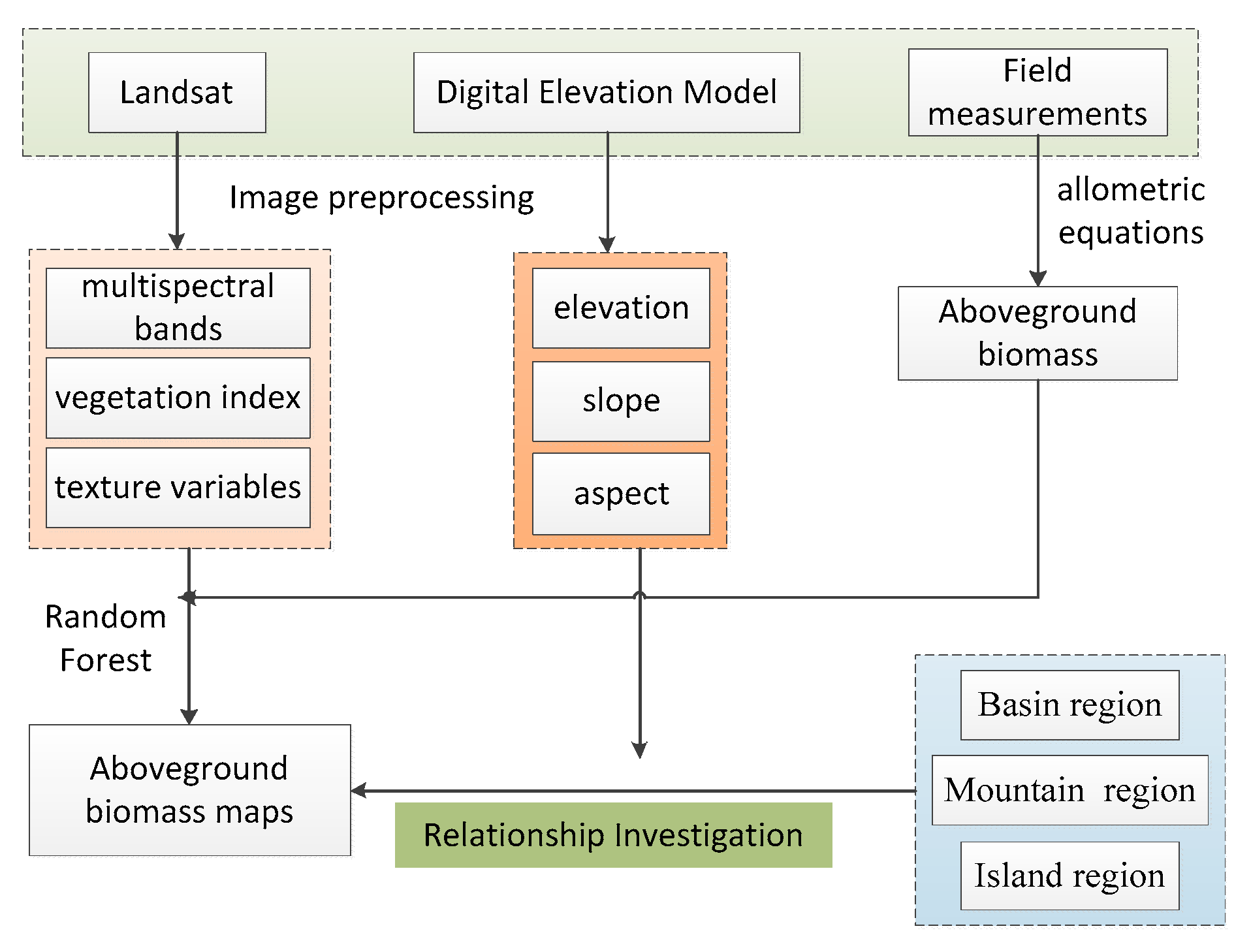
2. Materials and Methods
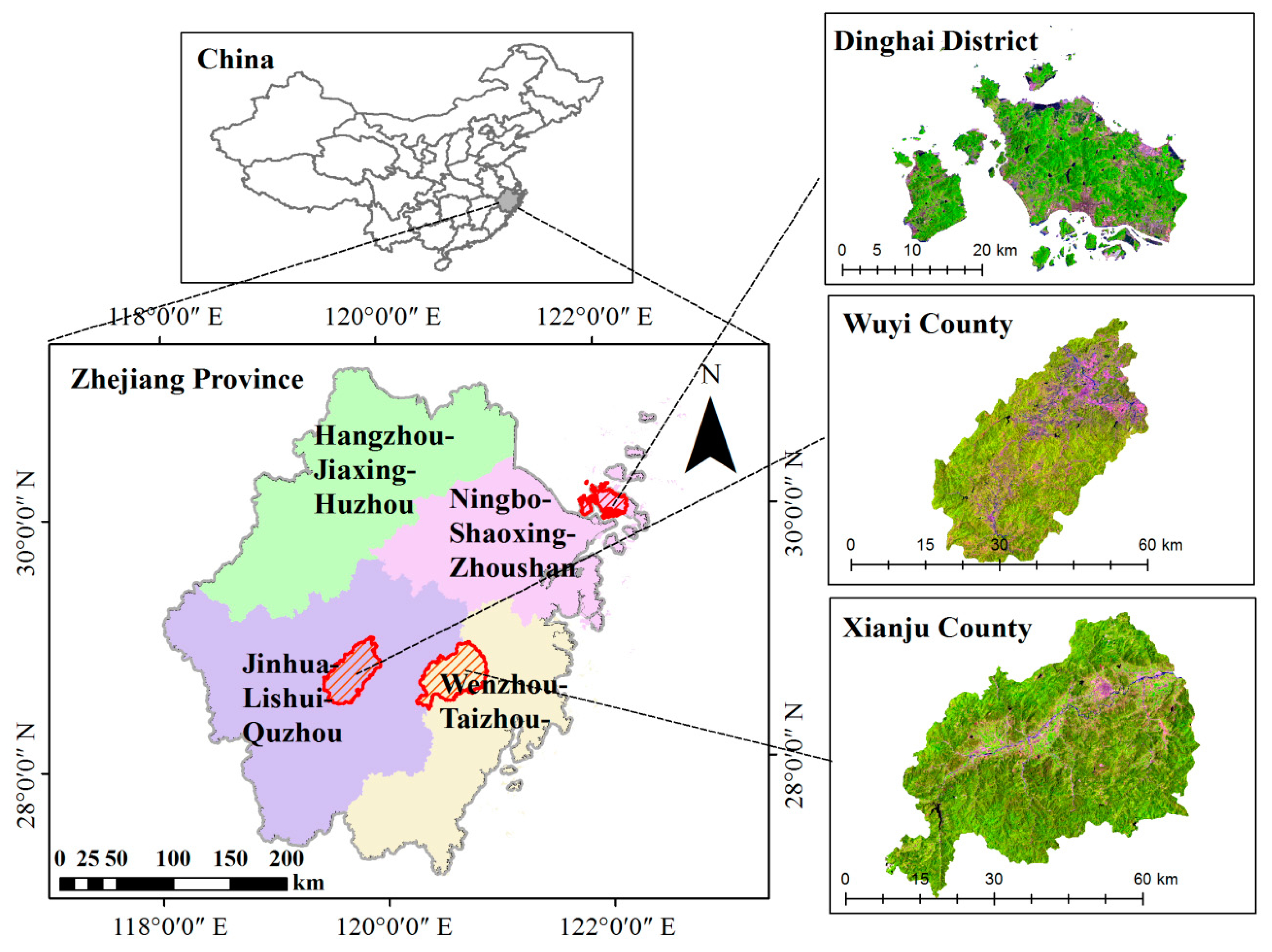
2.1. Study Area

Zhejiang Province is located in the southeastern region of China, ranging from 118°02′ E–123°08′ E, 27°03′ N–31°11′ N, with a subtropical monsoon climate. The annual average temperature is between 15 and 18 °C and the annual precipitation is between 1100 and 2000 mm. Being one of the most developed provinces with regard to the economy in China, it has consumed a large number of wood resources in the past several decades, and now, a majority of the land is covered with secondary forests. The local government has made great efforts to protect forests. As a result, the total forest coverage in the province has reached 60.91%. To investigate the influence of different topographic factors on AGB and its change, three counties named Wuyi County (administered by Jinhua City), Xianju County (belonging to Taizhou City), and Dinghai District (governed by Zhoushan City) were selected as the study areas (Figure 2). They are representative of basin, mountain, and island regions, which are located in the middle, southeast, and northeast of Zhejiang Province, respectively.

2.2. Field-Measured Data

Field investigations were carried out in 2010 and 2015 by Zhejiang Academy of Forestry. Sample plot design and selection were completed by taking into account the local geographical environment factors across the whole province. The size of each plot was 20 m × 20 m for trees, with three 2 m × 2 m subplots set in the diagonal line of each plot for shrubs and grasses [14]. The total biomass in each plot was calculated by summing the biomass of all trees, shrubs, and herbs, which was further defined as the final aboveground biomass (AGB) with a unit of Mg/ha. AGB values of broadleaved forests, coniferous, and broadleaved mixed forests, shrubs, bamboo forests, pine forests, and Chinese fir forests were calculated using measured DBH and height values embedded in specific allometric equations developed by Yuan et al. [26].
Quadrats outside the forest region and administrative boundary were deleted after checking their positions on remote sensing images and Google Earth based on visual interpretation. The outliers were selected and removed using the Pauta method, also named 3σ (standard deviation) measurement, by calculating the mean and variance values [20]. The statistics of the final dataset for subsequent analysis are shown in Table 1.

2.3. Remote Sensing Data

Landsat-5 Thematic Mapper (TM) and Landsat-8 Operational Land Imager (OLI) images (L1T) were downloaded from the United States Geological Survey (USGS) website [27]. Compared to the selected multispectral bands with a spatial resolution of 30 m, the thermal infrared channels for TM (120 m) and OLI (100 m) were abandoned for their coarser resolution. The first blue band (0.43–0.45 μm) of Landsat 8 OLI was removed to keep the bands consistent with Landsat 5 TM. The dates of the acquired images were almost in the same season by considering the phenology. Nevertheless, limited by the availability of cloudless images, the selections were based on the hypothesis that there was no significant biomass difference between imagery acquisition and field investigation. Detailed information about the Landsat images is listed in Table 2.
Digital Elevation Model (DEM) data were acquired from the Advanced Spaceborne Thermal Emission and Reflection Radiometer Global Digital Elevation Model (ASTER GDEM) V2 product with a spatial resolution of 30 m. Based on the DEM data, elevation, slope, and aspect were generated as the three basic geomorphology features. Administrative boundaries, present land use maps, forest maps, Google earth images, and socioeconomic statistics were collected as additional datasets.
To reduce the impact of the atmosphere, radiometric calibration was completed by inputting gain and offset information from the attached files, and an atmospheric correction using fast line of sight atmospheric analysis of spectral hypercubes (FLAASH) was executed. C correction was adopted as the topographic correction method to reduce the impact of terrain effects, especially for regions with shady slopes.

2.4. Biomass Estimation from Remote Sensing

2.4.1. Feature Derivation

Consequently, the pixels containing corresponding sample plots were selected to link the spectral information of Landsat imagery with the biomass density of quadrats based on the hypothesis that there should be no significant difference between the biomass per area in the 20 m × 20 m field plots and their position-homologous 30 m × 30 m Landsat pixels. Candidate predictor variables were extracted from the remote sensing imagery specific to previous studies, including multispectral bands, vegetation indices, and texture information. The corrected Normalized Difference Vegetation Index (NDVIc), incorporating shortwave infrared bands (SWIR), was calculated [28]. Three components, including brightness, greenness, and wetness, were also derived through the tasseled cap (TC) transformation [29]. Texture variables were also extracted using the gray-level co-occurrence (GLCM) method.

2.4.2. Machine Learning Method

Biomass data selected from field plots were considered as the response variable, and derivatives from remote sensing imagery were treated as predictive variables. Random forest was selected as the prediction method to establish the relationship between AGB and derivatives because numerous researchers have testified to this algorithm’s outstanding performance in biomass estimation [5,20,30]. The algorithm randomly selects variables at each node in the regression and classification tree and uses the bootstrap method to construct training samples without pruning. During this process, 2/3 samples are usually selected as training data, and the others are treated as validation data, which is also called “out-of-bag” [22]. The random selection of samples and variables makes the prediction results variable, but efficient. There are two important parameters, named mtry and ntree, that should be adjusted during the modeling process [31]. ntree controls the number of trees and is usually set to 500, while mtry determines the number of features and is usually set to 1/3 of the total number of input features. In addition, random forest is capable of estimating the relative importance of input features, which can be indicated by two built-in indices named %IncMSE and IncNodePurity. %IncMSE refers to Mean Decrease Accuracy and is calculated by constructing each tree of an ensemble with and without the specific variable. For all trees, the differences in error of these two variants are recorded, averaged, and normalized by their standard deviation [32,33]. It has been used in many previous studies [22] and was adopted in the current study.

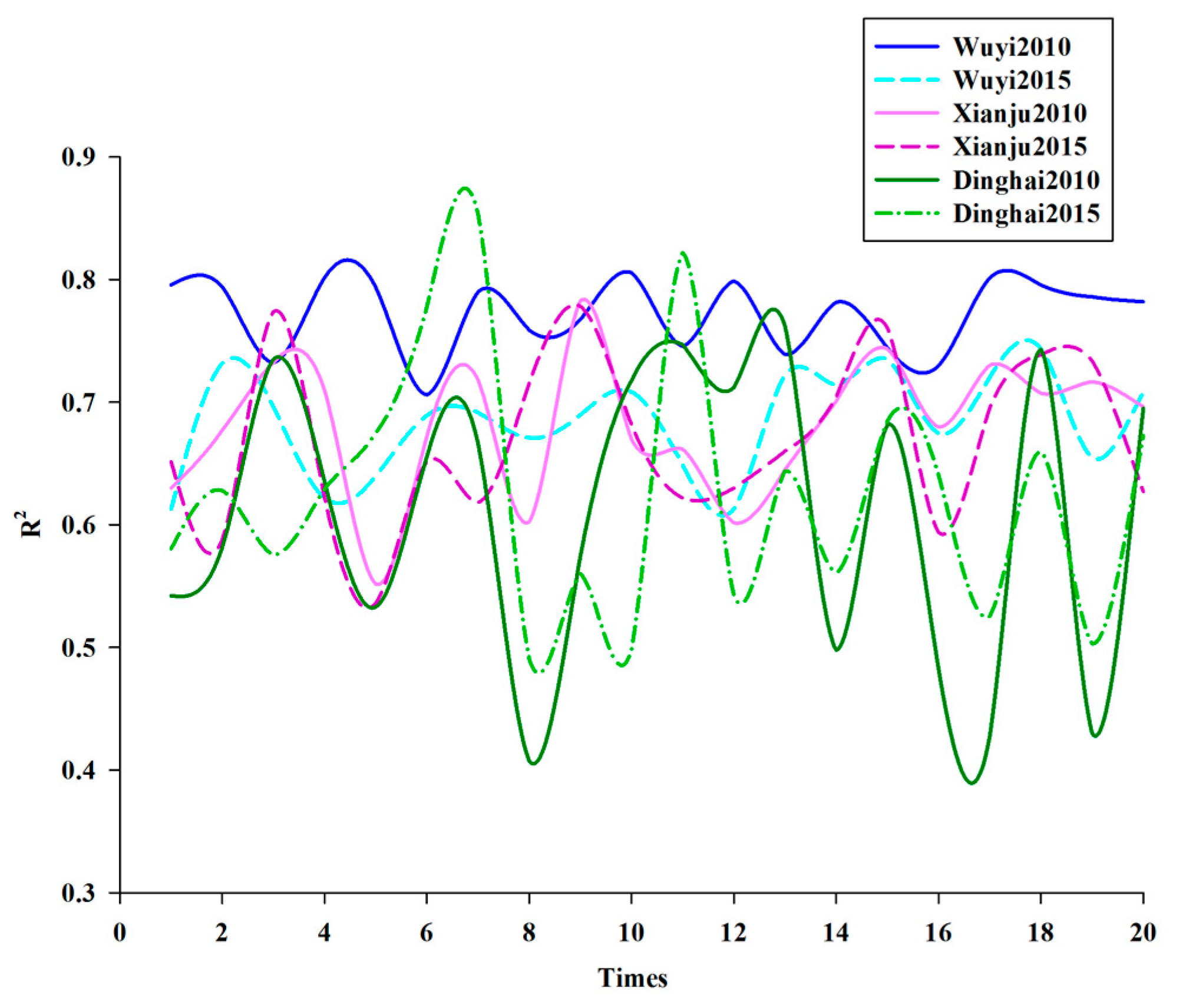
2.4.3. Precision Evaluation

Ten-fold cross-validation was selected as the accuracy assessment approach. It divided the dataset into 10 groups. Once one of the groups was selected as the validation set, the other groups were treated as the training set each time. The process was repeated 10 times until all the groups had been traversed. Random forest modeling and accuracy assessment were implemented in the R 3.5.1 © open source software through the “caret” package [34]. R2 values indicating the variance in the response variable explained by the predictor variables were computed to evaluate modeling accuracy. Furthermore, scatter diagrams of predicted and field-measured biomass values were plotted.

2.5. AGB Mapping and Spatio-Temporal Characteristic Analysis

To improve the accuracy of identification, a hierarchical system with six categories (0–30, 30–60, 60–90, 90–120, 120–150, >150 Mg/ha) used in Zhao et al.’s study was applied to the estimated AGB maps in all regions [6]. Simultaneously, topographic variables including elevation, slope, and aspect were classified into different levels by referring to Du et al.’s work [25]. Elevation was reclassified with an interval of 200 m for Wuyi and Xianju. Considering the relative lower elevation in Dinghai District, an interval of 50 m was set by consulting the work of Pan et al. [35]. In terms of slope and aspect, six grades of slope (0–5°, 5–15°, 15–25°, 25–35°, 35–45°, and >45°) and eight categories of aspect (north, northeast, east, southeast, south, southwest, west, northwest) were adopted to investigate the influence of slope and aspect on AGB distribution and its change. Meanwhile, mean values for each category were calculated from the estimated AGB maps for comparison. Besides, regression methods were used to check whether there was significant correlation between AGB/change and corresponding topography variables.

3. Results

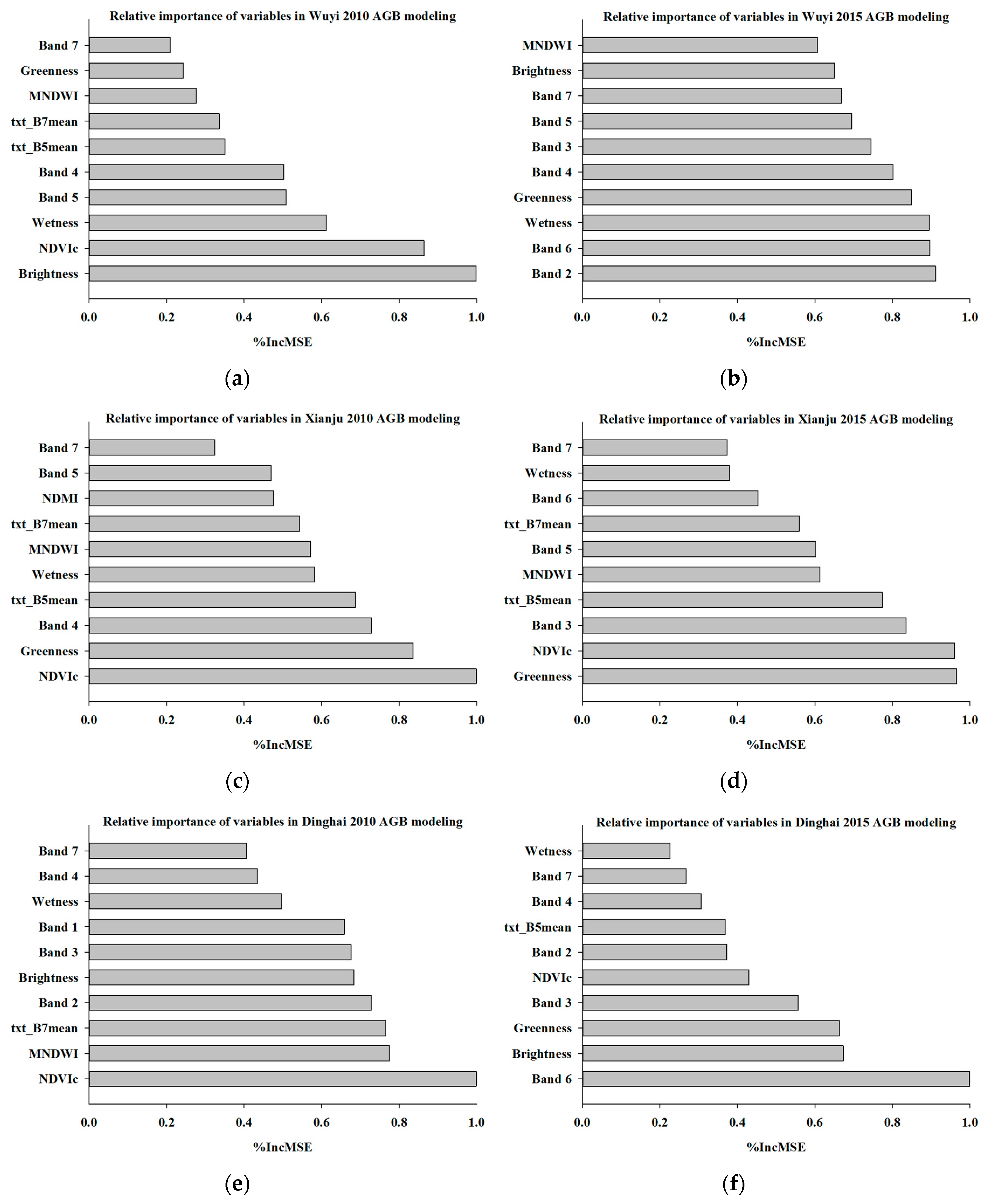
3.1. The Importance Rank of Variables

Due to the randomness of the random forest algorithm, all the modeling process had to be repeated 20 times [20,36]. To investigate the performance of different variables involved in biomass estimation, %IncMSE were normalized for more convenient comparison [36], and the top 10 variables participated in the modeling process in three regions were selected to form the rank of the most important variables shown in Figure 3. Among all the selected variables, NDVIc was always selected as the most significant predictor in 2010, but the SWIR band (OLI Band 6) and derivatives from tassel transformation were among the best in 2015.

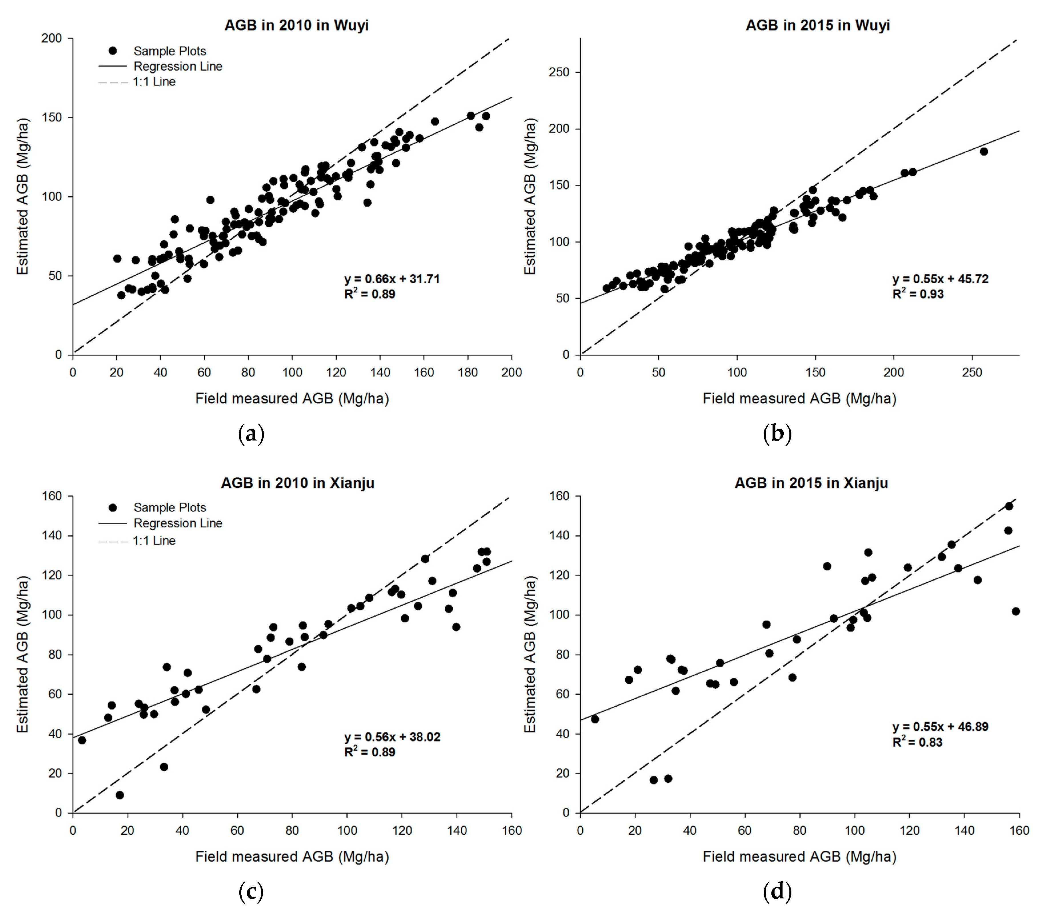
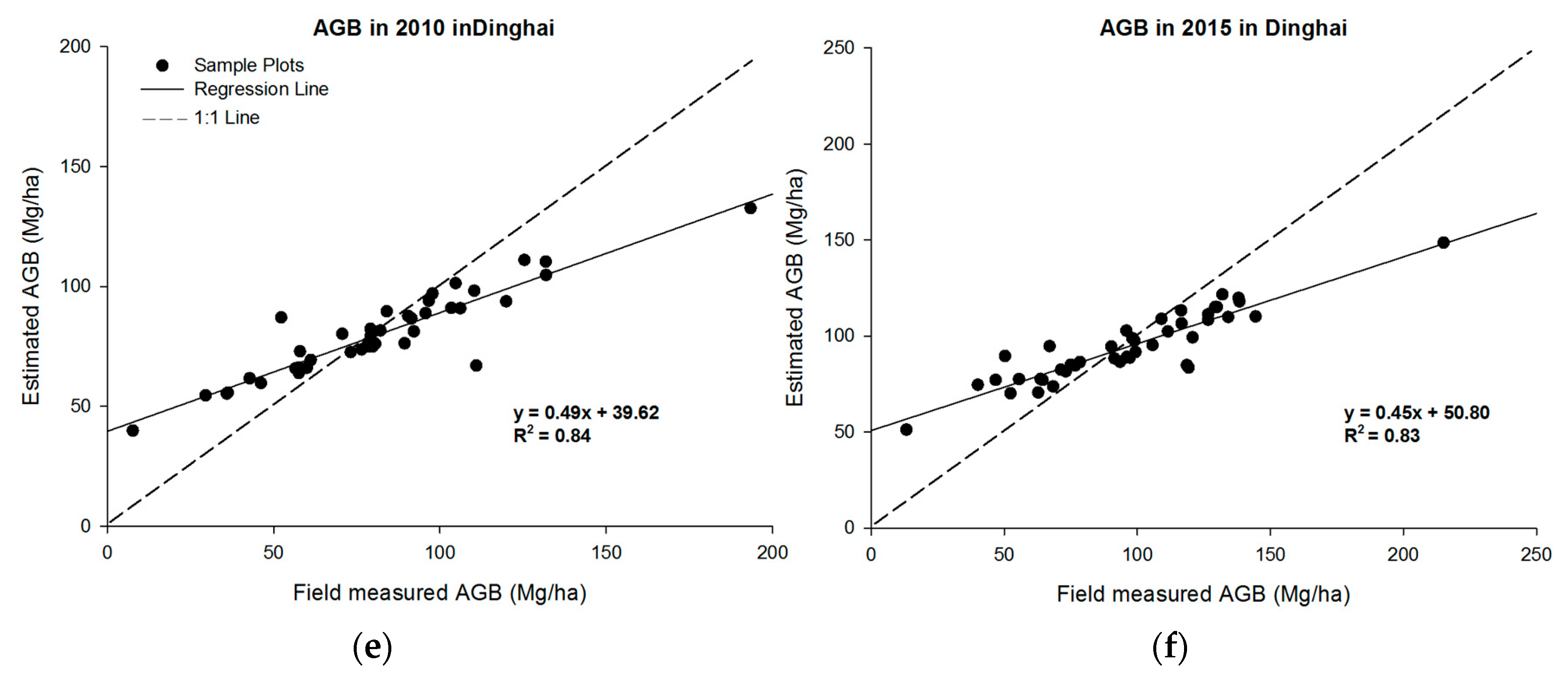
3.2. Accuracy Assessment

All the samples were used to predict the AGB as a previous study had found that using all samples, when compared to a smaller sample size, was propitious to biomass estimation [5]. R2 were calculated to inspect the modeling accuracy (Figure 4). It can be seen that R2 values fluctuated with different magnitudes, where the estimation in 2010 in Wuyi County (blue, solid line) obtained the best performance, while the prediction in Dinghai (green) showed relatively lower accuracy. Besides, Figure 5 shows the scatter plots by using the simple linear regression method for estimated AGB and field measurements. Limited by the total number of samples, Xianju and Dinghai had lower R2 values than Wuyi, but all values of R2 were beyond 0.8. Meanwhile, underestimation of the values of the highest biomass and overestimation on the values of the lowest biomass cannot be ignored.

3.3. Bitemporal Distribution and Change of Aboveground Biomass

When inspecting the spatial change in different periods, Figure 6 showed that the overall AGB in three regions increased from 2010–2015. AGB values below 30 Mg/ha accounted for a relatively small proportion in all the regions, which were mostly distributed in water areas and construction lands (when compared to the land use map, but not shown here). Simultaneously, AGB values beyond 150 Mg/ha also occupied a low percentage, and AGB in most regions changed in the range of 30–120 Mg/ha. Moreover, AGB in Dinghai District increased evidently, almost covering the whole region.
The topographic features in the three regions in Table 3 indicated that Dinghai District, occupying the smallest area, had the lowest mean values of elevation, slope, and aspect, while Xianju County, covering the largest area, owned the highest mean values. Meanwhile, Wuyi and Xianju Counties had higher mean values of AGB than Dinghai District had both in 2010 and 2015. However, the AGB in Xianju County acquired the least increase with the minimum increase rate, and Dinghai had the highest increase rate of AGB.

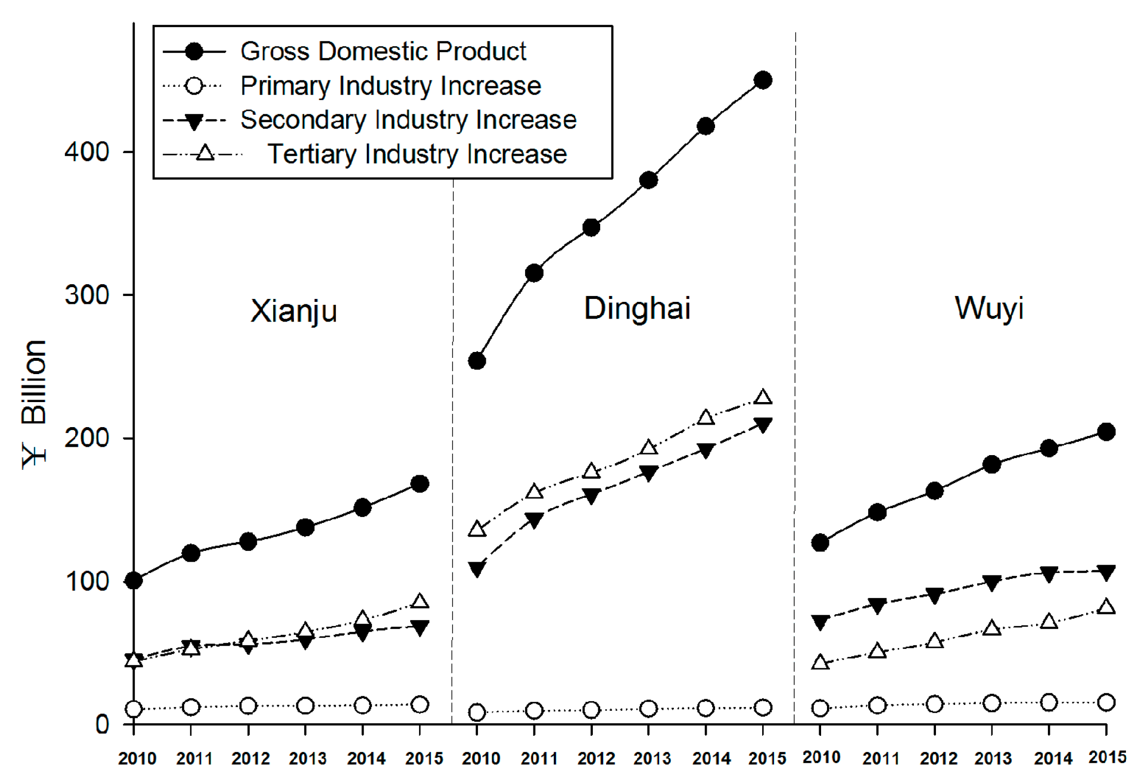
3.4. Spatiotemporal Biomass Change in the Three Regions

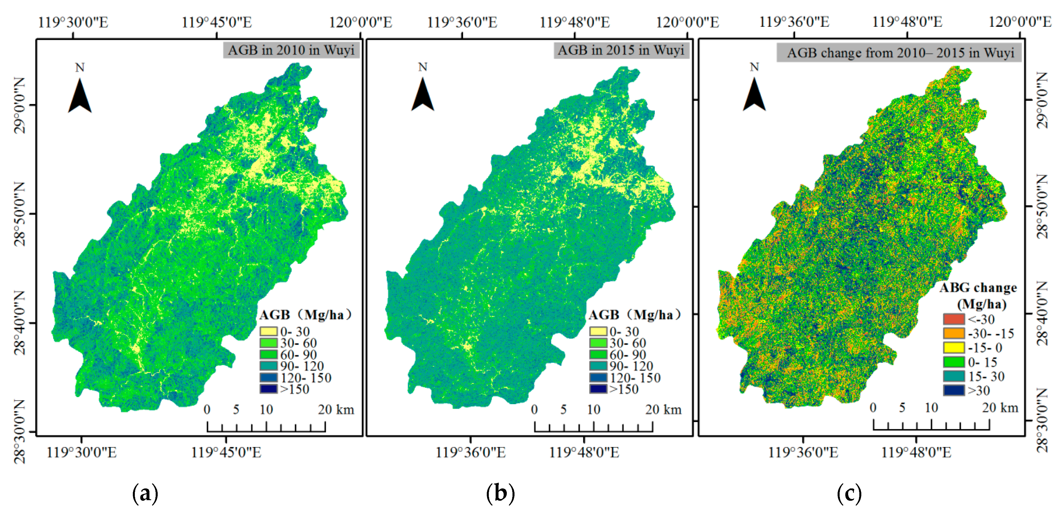
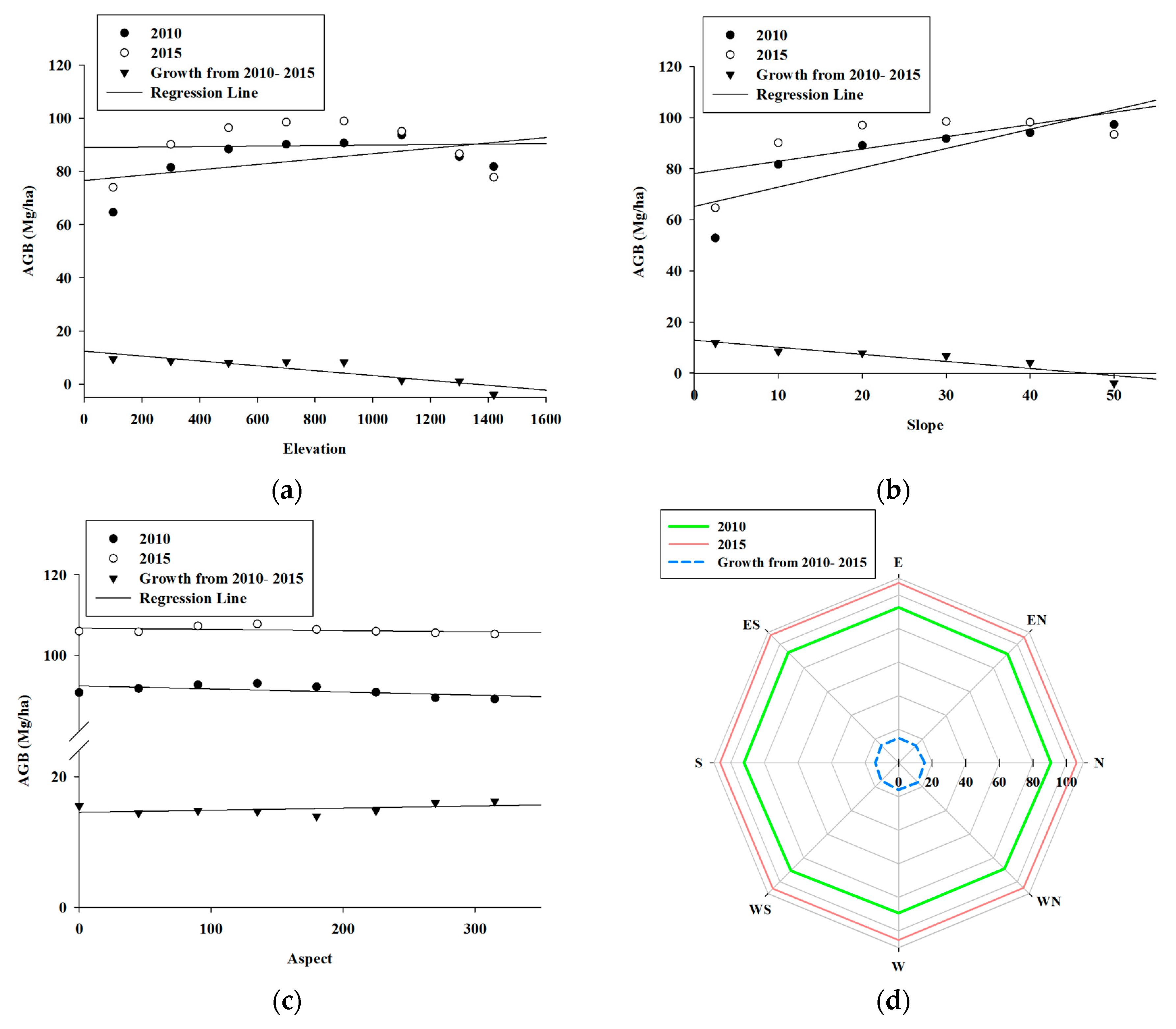
3.4.1. AGB Change in Wuyi County

Figure 7 showed that the relations between AGB/change and terrain features in Wuyi County had different trends. When the elevation became higher, AGB gradually grew until the elevation reached 900 m, then it started to decrease with higher elevation. This situation took place both in 2010 and 2015. Although in general, AGB increased with higher elevation, the magnitude of biomass increase was getting smaller (Figure 7a). In terms of slope (Figure 7b), a higher slope possessed higher biomass values, but a steeper slope made lower AGB increase, especially when the slope was higher than 45°; AGB in 2015 was obviously smaller than that in 2010. As for the aspect, Figure 7c shows that the mean values of AGB were almost similar in both years; even the change during this period in different aspects was almost the same. The radar chart (Figure 7d) provides more information to understand the AGB distribution characteristics for eight aspects, where all the octagons had nearly equal angles. No significant AGB difference could be found for different aspects, which was verified by the regression methods displayed in Table 4. It was also demonstrated that the magnitude of AGB increase had significant negative correlations with elevation and slope.

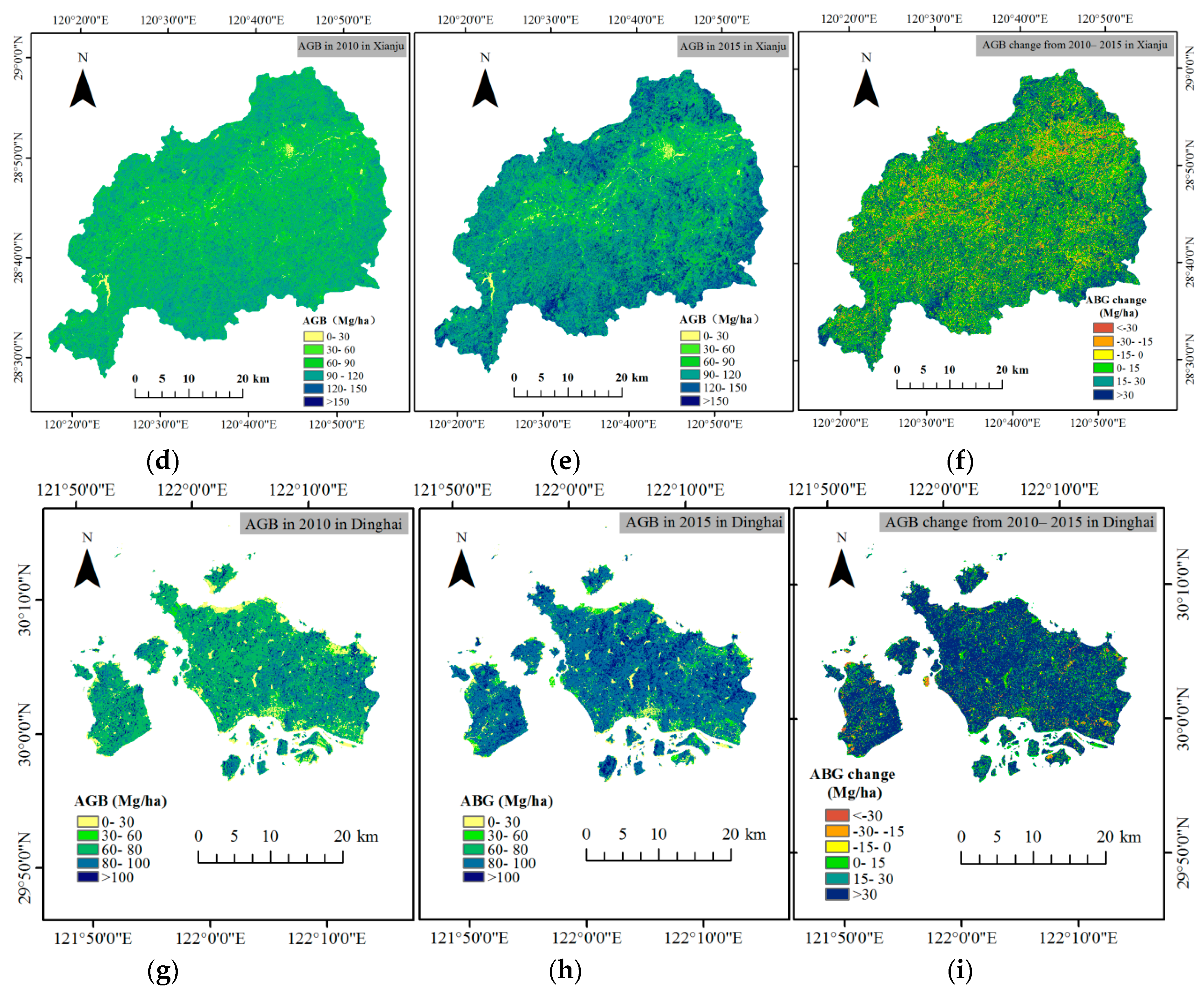
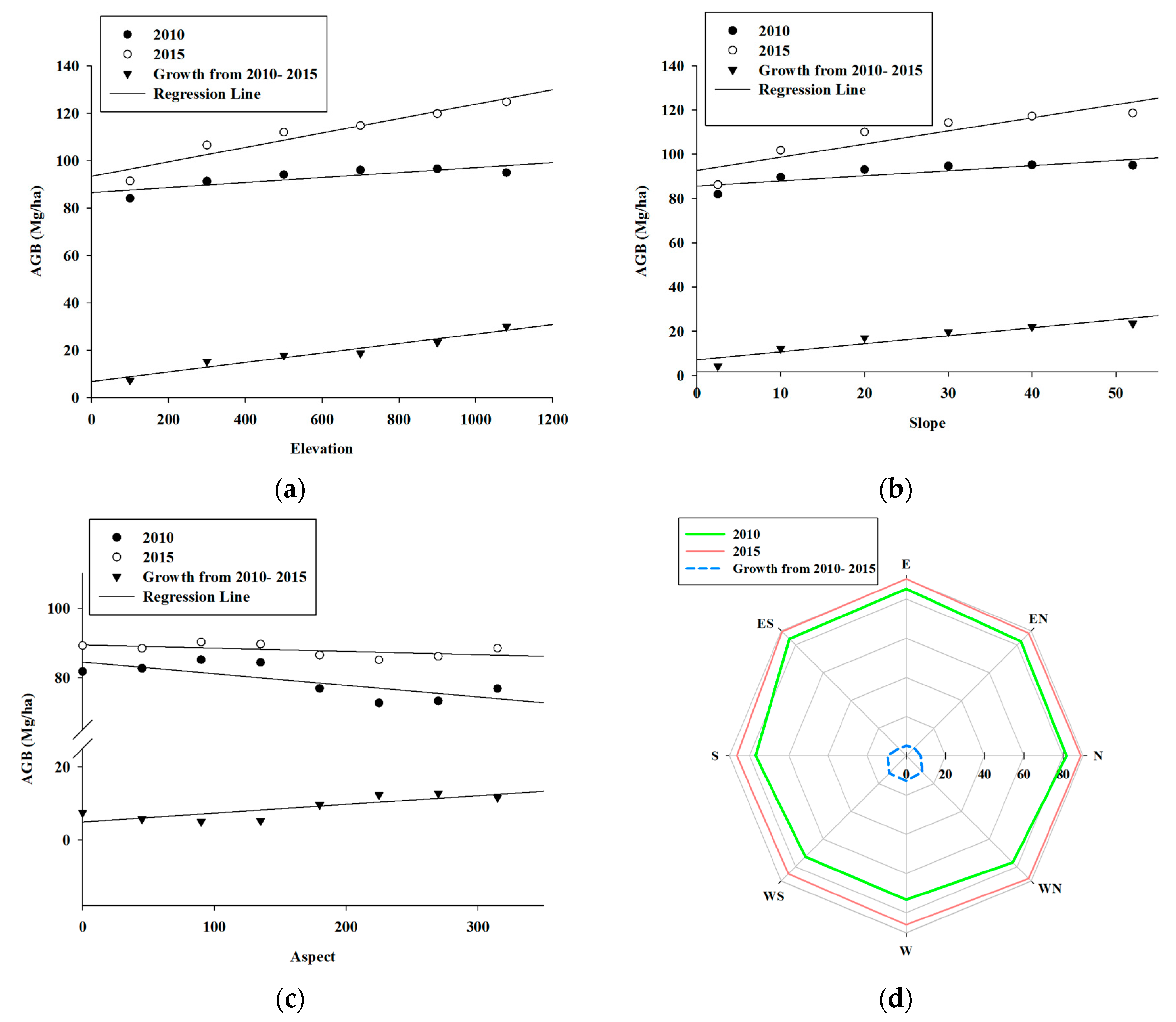
3.4.2. AGB Change in Xianju County

The relation between AGB/change and terrain features in Xianju County is displayed in Figure 8. Figure 8a,b indicates that biomass increased with higher elevation and a steeper slope both in 2010 and 2015, but Figure 8c states that aspect had different relationships with biomass in these two years. Combined with the results in Table 5, AGB and its increase had a positive relation with elevation and slope. Meanwhile, AGB had a significant negative relation with aspect in 2010, but the relationship became insignificant in 2015 (Figure 8c). On the basis of the result in the radar chart (Figure 8d), AGB acquired a higher increase in magnitude in the western aspects.

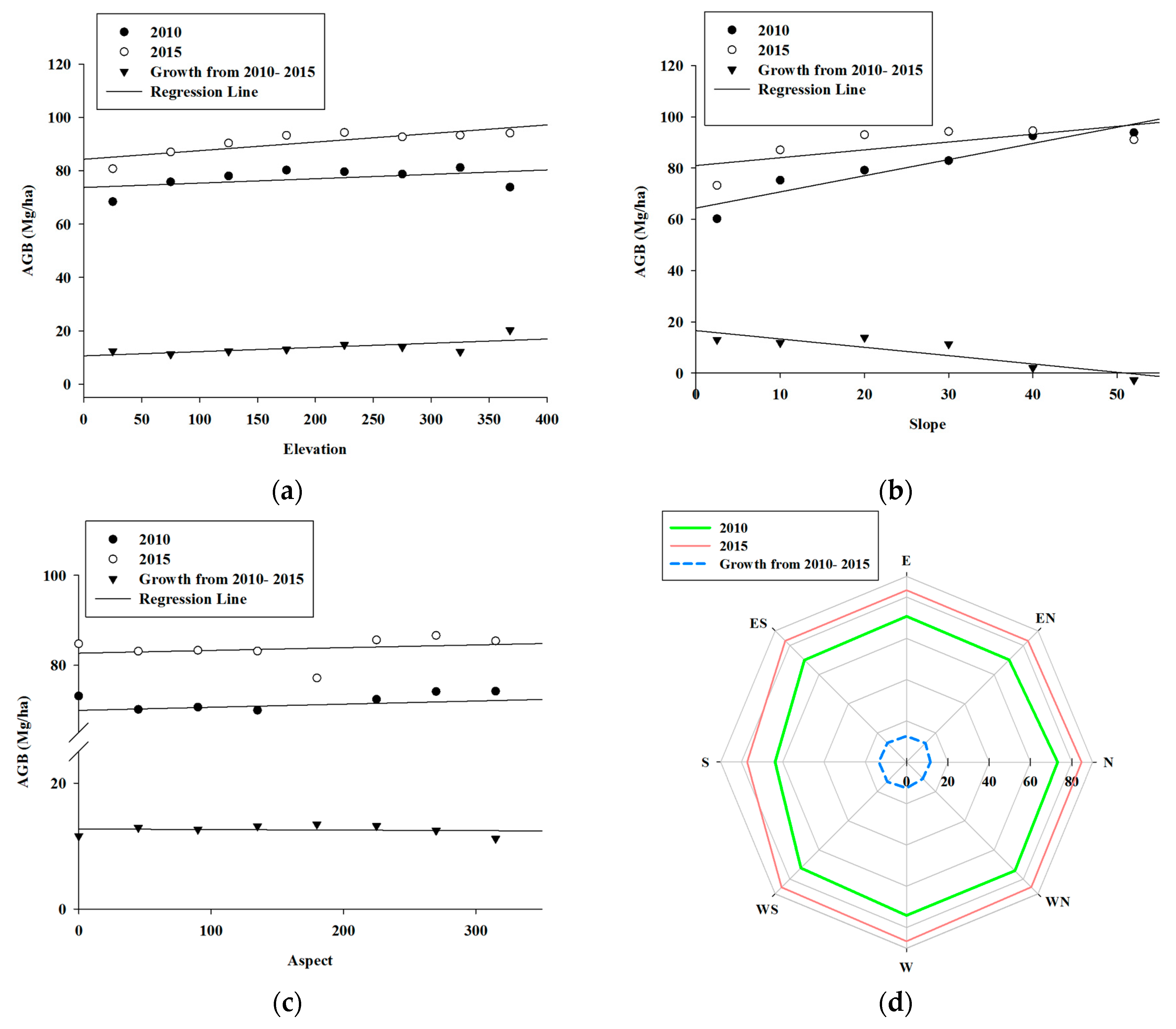
3.4.3. AGB Change in Dinghai District

From Figure 9, different relations can be found between AGB/change and three topographic factors. Connecting the results of Figure 9a to Table 6, it can be seen that AGB and its change increased with high elevation, but in 2010 and from 2010–2015, the linear correlations were not significant. When inspecting the slope, AGB generally increased with higher slope in each year, but when the slope became steeper, AGB changed with a lower increase un magnitude, especially when the slope was higher than 50°; AGB in 2015 was smaller than 2010 (Figure 9b). Although Figure 9c revealed that in the south aspect, AGB had the lowest value both in 2010 and 2015, the regression results (Table 6) affirmed that aspect had no significant relations with AGB in two years, and AGB kept at a relatively steady level during this period.

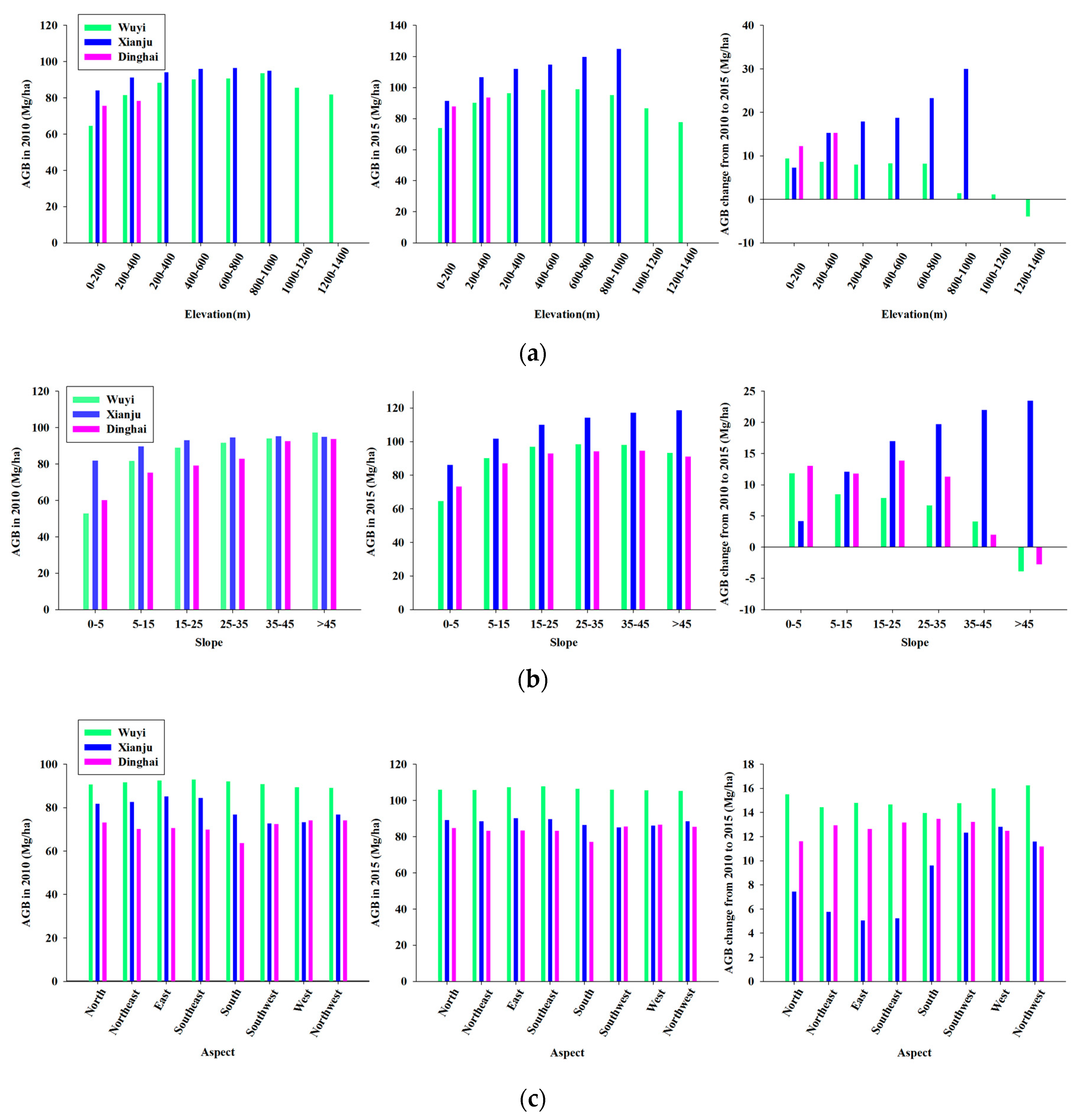
3.4.4. Comparison of AGB/Change in Three Regions

To investigate the AGB difference between the three terrain regions scientifically, the values of AGB/change were compared under the same assessment system using a unified stratified classification (Figure 10). Figure 10a shows that the mountains in Wuyi County had the highest elevation beyond 1000 m and Dinghai District held the lowest elevation. However, Xianju County always possessed the highest AGB in each subclass with a considerable magnitude of increase. AGB change in Wuyi in the period from 2010–2015 showed a decrease tendency when the elevation was higher, while in the other two regions, AGB obtained the opposite trend. In terms of slope, Xianju stood out for its notably higher AGB in 2015 among all the stratifications. Besides, when the slope became steeper, AGB increased with less magnitude in Wuyi and Dinghai, and it even became a negative number when the slope was larger than 45 degrees. However, the increase of AGB in Xianju kept growing during this period, independent of the change of slope (Figure 10b). As for the aspect, it can be observed from Figure 10c that Wuyi had the highest AGB and Dinghai had the lowest AGB in each aspect, both in 2010 and 2015. Furthermore, three regions all achieved increased AGB in all aspects, with Wuyi having the highest magnitude, but Xianju holding the least growth in each aspect.

4. Discussion

4.1. Comparison of Variable Importance

The relative importance of different variables involved in the modeling process is normalized and compared in Figure 3. Among the most important variables in 2015, except for that in Xianju, SWIR (OLI Band 6) held relatively higher score values of %IncMSE, which can be explained by the reason that SWIR is more sensitive to moisture and shade components inherent in the forest stand structure and less impacted by atmospheric conditions [6,37]. Moreover, NDVIc incorporating SWIR acquired better performance in 2010 than it did in 2015 for all regions, which suggested that it would be apt to support the hypothesis that this variable was more suitable for open forest stands [28,38]. The preceding presentation showed that AGB generally increased from 2010–2015, while here, the relative importance of NDVIc descended on the whole. In terms of tasseled cap, its components have been widely used in biomass estimation [14,21,39]. Brightness, greenness, and wetness were successively selected as important predictor variables, similar to other Landsat-related biomass estimation research [40]. However, it has been stated that Landsat 8 has a refined near-infrared spectral band for more accurate spectral acquisition when compared to the Landsat former series [11], but the advantage in the near-infrared band of OLI Band 5 over TM Band 4 remains to be further investigated.

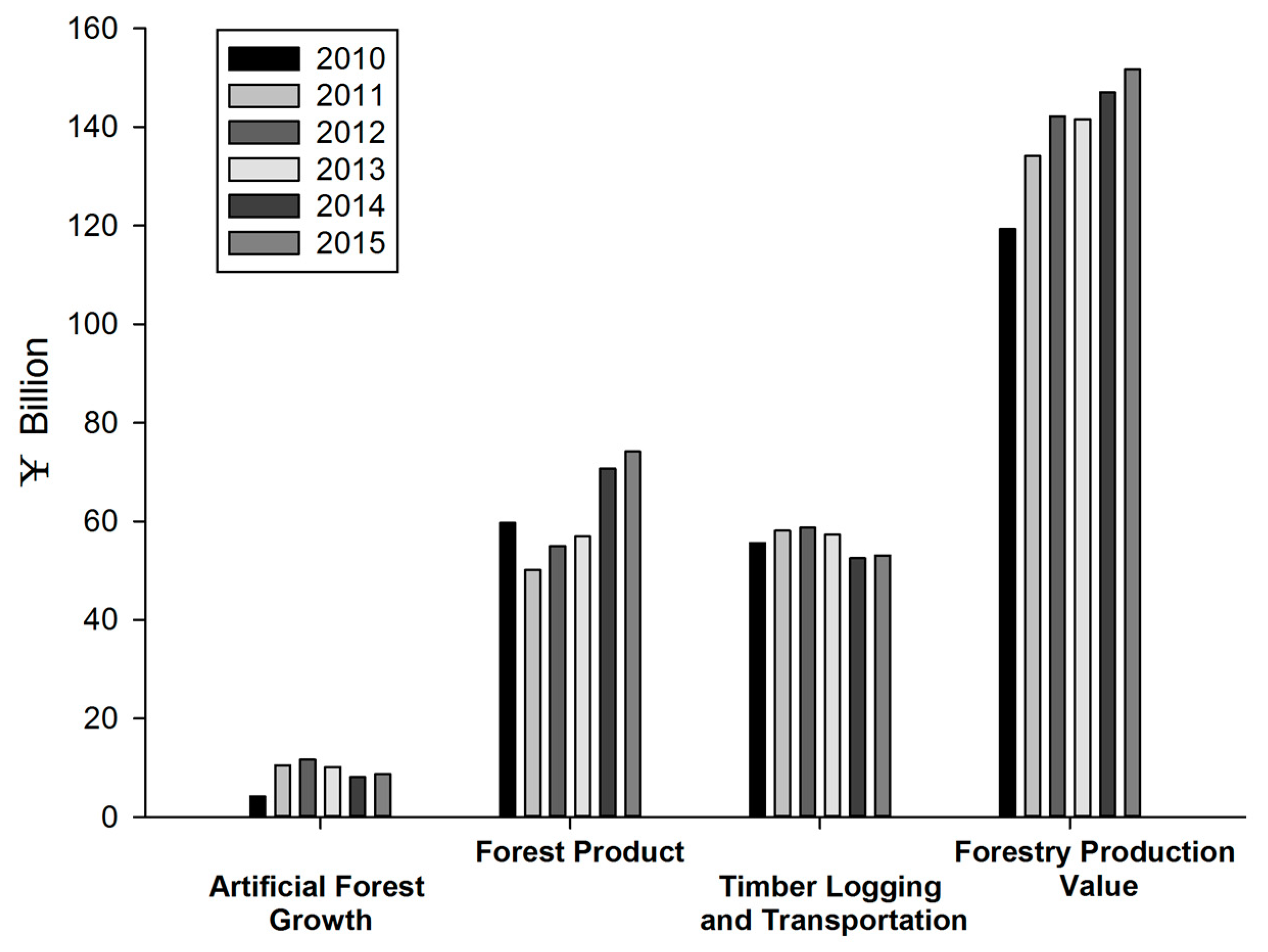
4.2. The Effect of Forest Policy on Biomass Spatiotemporal Variations

The total afforested area in Zhejiang Province increased from 2010–2012, but slightly decreased from 2013–2015 (Table 7). In addition, the total forestry production value increased from 2010–2015 (Figure 11). This implies that afforestation in the future will be limited by the finite area of land resources combined with rapid socioeconomic consumption, which indicates that the configuration characteristic of Zhejiang forests will change from quantity augmentation to quality improvement. Biomass is defined as the total amount of organic matter present at a given time per unit area and is the foundation of energy and nutrient exchange for forest ecosystem. Therefore, it is usually treated as an important indicator of forest quality, and the results of our previous study showed that forest policy implementation of ecological forests was beneficial for the increase of biomass [9]. Thus, proper management such as establishing nature reserves, implementing forest protection policies, and enhancing public awareness of forest ecological benefit would have a powerful effect on the spatial change of biomass.
In this context, forest protection campaigns such as plain greening and ecological forests, which promote afforestation and prohibit deforestation, will provide a better environment for biomass accumulation and in some way explain the general increasing tendency of AGB in our study area. The government of Wuyi County delimited the ecological forest in 2001, and up to September 2010, the provincial ecological forest reached 42,894.89 ha, which accounted for 44.72% of the total forested land area in Wuyi [41]. It holds a larger proportion of mountain areas with relatively high forest age that promote higher biomass density. Comparably, there has been 18,996.21 ha of ecological forest in Dinghai District until 2015, holding a proportion of 64.2% [42]. Additionally, Xianju is one of the earliest pilot counties in Zhejiang province to implement the ecological forest program. Therefore, all of these measures would facilitate biomass increase.

4.3. The Terrain Impact on Biomass Distribution and Change

Biomass distribution is effected by many factors. In this study, we focus on the relationship between AGB and three important topographic factors including elevation, slope, and aspect among different regions. By summing up the above results, some interesting points have been found.
For the elevation feature, AGB in the three regions had a positive correlation with elevation more or less, especially for Xianju County. At the same time, it should be pointed out that when the elevation was higher, the AGB change obtained quite different trends in the three regions, where Wuyi, Xianju, and Dinghai had negative, positive, and insignificant correlations with elevation, respectively. As stated in the study of Zhang et al. [43], the property of main local tree species largely determined the characteristics of biomass spatial and temporal variation. There is a great percentage of broad forest in Xianju County, especially for the locations in the ecological forest, whose community composition containing large broadleaf species is mainly distributed at higher altitudes with better hydrothermal conditions. This may be the reason why in this region, AGB increases faster in higher mountains than that in flat areas. However, in Wuyi, a possible reason to explain why lower regions have a larger magnitude of AGB increase is that forest management activities like plain greening and ecological forest construction have been implemented [41]. Furthermore, the relatively limited elevation with a highest elevation below 400 m and the surrounding sea and ocean environment lead AGB in Dinghai to have a weakened relation with elevation.
With regard to slope, AGB/change in the three regions had significant relations with slope to varying degrees. Both in 2010 and 2015, AGB in Wuyi, Xianju, and Dinghai had a positive relation with slope. Du et al. assumed that vegetation distributed in higher slopes avoided the frequent intervention of human activity, and could be better preserved, contributing to more plentiful forest growth that promoted biomass accumulation [25]. However, in Wuyi and Dinghai, AGB acquired a negative increase when the slope was larger than 45°.
When it comes to aspect, it seems that aspect only had a significant correlation with AGB/change to some extent. Aspects in the south, southwest, west, and northwest are called sunny slopes [44,45], and AGB in these aspects achieved a larger magnitude of increase in Xianju. However, AGB at different aspects in Wuyi and Dinghai had no distinct difference. Comparably, aspect had the lowest relation with AGB and its change among the three topographic factors.
When comparing the relative importance of the three terrain parameters, elevation and slope both played significant roles in temporal AGB change. Although all features influenced AGB in Xianju, a typical mountainous area, elevation was at the top of the list. By comparison, slope was inclined to be the most important determinant for the island region of Dinghai. In Wuyi, slope also had a relatively more significant relation with AGB. Despite this, at the provincial level, Du et al. found that forest carbon density increased with higher altitude in Zhejiang Province [25]. The situation becomes complicated when the provincial scale changed to smaller regional scales. In our study, unambiguous principles to explain the AGB-terrain relationship in the three regions are still needed in further investigations, as a number of studies has found that topography is closely related to solar radiation, temperature, moisture, and soil condition, all these interrelate with vegetation growth and human activities [9,46,47]. The objective of this study was to reveal the relationship between AGB/change and topography factors, while the spatiotemporal characteristics of AGB should be explained by the combination of natural condition and anthropogenic behavior.

4.4. Future Works

Although the spatial AGB maps in different periods were produced and the characteristics of AGB/change were analyzed, further studies should be conducted in the future. First, TM images for Wuyi County (in May and October) and Xianju County (in 2007) were an expedient selection restricted by the coverage of clouds, as mentioned above. Strictly speaking, remote sensing data should be selected by referring to field data to ensure that both were collected from the same period. Second, total biomass should include tree trunks, branches, and foliage, but the optical imagery we used captured only the signals from the vegetation canopy, and even contained noise from soil and other environmental backgrounds, which resulted in great uncertainty in the biomass estimation. Lidar has been widely used as it has the ability to provide vertical information that is closely related to AGB [48,49]. Third, the random forest algorithm was used to produce the AGB map and rank the relative importance of selected variables, but it is still a black box in which the interaction mechanism between remote sensing data and forest biochemical parameters is unrevealed. Approaches with more distinct mechanisms can be explored. Fourth, limited by our available forest investigation dataset, a typical region representing plain terrain in the north of Zhejiang has not be included to form a more comprehensive comparison. Fifth, time series biomass estimation should be used instead of bi-temporal biomass change to find more valuable and detailed information [50]. It should be noted that in this study, the mean aboveground biomass density in Dinghai district was the lowest, but when investigating the industrial structure in three regions, Dinghai had the highest GDP (gross domestic product) during 2010–2015 (Figure 12). Therefore, more frequent remote sensing imagery can be explored to find out whether a correlation exists between biomass and socioeconomic factors.

5. Conclusions

The distribution of aboveground biomass changes with various natural and anthropogenic environment conditions. Remote sensing provides a nondestructive and efficient way to describe the temporal and spatial characteristics of this information and has earned increased attention in recent years. In this study, Landsat imagery covering three regions in Zhejiang Province, China, was collected, representative of different topographic regions including basin, island, and mountain areas. Combined with field-measured plots, bi-temporal aboveground maps (2010 and 2015) were produced based on the random forest algorithm. The spatial distributions and changes in AGB were investigated and analyzed through establishing stratified topographic categories based on DEM data. As a result, the biomass in all regions increased from 2010–2015. In the basin region that had more frequent human activities, forests in lower-altitude regions had higher biomass increases. In the mountain region, AGB was uppermost influenced by elevation, and forests at higher elevations acquired both a higher value and an increased magnitude. For the islands, with limited elevation and water surrounding environment, the dominant influence for AGB/change was inclined to be the slope. Comparatively speaking, aspect had the weakest relation with AGB. More works should be done to clarify the complex relationships between AGB and diverse terrain conditions.
The local government of Zhejiang Province has taken such actions as plain greening and ecological forest implementation to promote the increase of forest coverage and prevent deforestation, which is beneficial to regional forest ecosystems. In the future, with the excavation of limited potential forests, the improvement of forest quality should be the focus of forest management. Biomass is an important parameter for forest ecosystem assessment. As shown by this study, the interaction between natural conditions and human activities, which cannot be completely separated, exerts considerable influence on local forests. Remote sensing-based biomass estimation, with especial attention paid to regional heterogeneity, can provide scientific guidance for natural resource management.

Author Contributions

Conceptualization, A.S. and C.W.; methodology, C.W.; investigation, A.S., B.J., W.Y. and C.W.; data curation, A.S., C.W., S.H., E.Z. and Y.L.; writing, original draft preparation, A.S. and C.W.; writing, review and editing, J.D. and K.W.; funding acquisition, A.S., C.W., B.J., W.Y. and C.W.

Funding

This research was funded by the Key Research & Development Program of Zhejiang Province, China (No. 2017C02028) and the Open Fund of the Institute of Agricultural Remote Sensing and Information Technology of Zhejiang Province (No. ZJRS-2017004).

Acknowledgments

The authors are appreciative of the USGS and NASA for the open archives of Landsat imagery, and we would like to acknowledge the R Development Team for the open-source package used for the statistical analysis. The authors thank Qiming Zheng at Zhejiang University for his constructive comments, suggestions, and help in enhancing this manuscript. The authors thank the Editor and two anonymous reviewers for their constructive comments, suggestions and help in enhancing the manuscript.

Conflicts of Interest

The authors declare no conflict of interest.

References

  1. Pan, Y.; Birdsey, R.A.; Fang, J.; Houghton, R.; Kauppi, P.E.; Kurz, W.A.; Phillips, O.L.; Shvidenko, A.; Lewis, S.L.; Canadell, J.G. A large and persistent carbon sink in the world’s forests. Science 2011, 333, 988–993. [Google Scholar] [CrossRef]
  2. Shuman, J.K.; Shugart, H.H.; Krankina, O.N. Assessment of carbon stores in tree biomass for two management scenarios in Russia. Environ. Res. Lett. 2013, 8, 045019. [Google Scholar] [CrossRef] [Green Version]
  3. Lu, D.; Chen, Q.; Wang, G.; Liu, L.; Li, G.; Moran, E. A survey of remote sensing-based aboveground biomass estimation methods in forest ecosystems. Int. J. Digit. Earth 2014, 1–43. [Google Scholar] [CrossRef]
  4. Pflugmacher, D.; Cohen, W.B.; Kennedy, R.E.; Yang, Z. Using Landsat-derived disturbance and recovery history and lidar to map forest biomass dynamics. Remote Sens. Environ. 2014, 151, 124–137. [Google Scholar] [CrossRef]
  5. Fassnacht, F.E.; Hartig, F.; Latifi, H.; Berger, C.; Hernández, J.; Corvalán, P.; Koch, B. Importance of sample size, data type and prediction method for remote sensing-based estimations of aboveground forest biomass. Remote Sens. Environ. 2014, 154, 102–114. [Google Scholar] [CrossRef]
  6. Zhao, P.; Lu, D.; Wang, G.; Wu, C.; Huang, Y.; Yu, S. Examining Spectral Reflectance Saturation in Landsat Imagery and Corresponding Solutions to Improve Forest Aboveground Biomass Estimation. Remote Sens. 2016, 8, 469. [Google Scholar] [CrossRef]
  7. Wang, X.; Shao, G.; Chen, H.; Lewis, B.J.; Qi, G.; Yu, D.; Zhou, L.; Dai, L. An Application of Remote Sensing Data in Mapping Landscape-Level Forest Biomass for Monitoring the Effectiveness of Forest Policies in Northeastern China. Environ. Manag. 2013, 52, 612–620. [Google Scholar] [CrossRef]
  8. Roy, D.P.; Wulder, M.A.; Loveland, T.R.; Woodcock, C.E.; Allen, R.G.; Anderson, M.C.; Helder, D.; Irons, J.R.; Johnson, D.M.; Kennedy, R.; et al. Landsat-8: Science and product vision for terrestrial global change research. Remote Sens. Environ. 2014, 145, 154–172. [Google Scholar] [CrossRef]
  9. Wu, C.; Shen, H.; Wang, K.; Shen, A.; Deng, J.; Gan, M. Landsat Imagery-Based Above Ground Biomass Estimation and Change Investigation Related to Human Activities. Sustainability 2016, 8, 159. [Google Scholar] [CrossRef]
  10. Zhu, X.; Liu, D. Improving forest aboveground biomass estimation using seasonal Landsat NDVI time-series. ISPRS J. Photogramm. 2015, 102, 222–231. [Google Scholar] [CrossRef]
  11. Dube, T.; Mutanga, O. Evaluating the utility of the medium-spatial resolution Landsat 8 multispectral sensor in quantifying aboveground biomass in uMgeni catchment, South Africa. ISPRS J. Photogramm. 2015, 101, 36–46. [Google Scholar] [CrossRef]
  12. Baret, F.; Buis, S. Estimating Canopy Characteristics from Remote Sensing Observations: Review of Methods and Associated Problems. In Advances in Land Remote Sensing; Springer: Dordrecht, The Netherlands, 2008. [Google Scholar]
  13. Verrelst, J.; Camps-Valls, G.; Muñoz-Marí, J.; Rivera, J.P.; Veroustraete, F.; Clevers, J.G.P.W.; Moreno, J. Optical remote sensing and the retrieval of terrestrial vegetation bio-geophysical properties—A review. ISPRS J. Photogramm. Remote Sens. 2015, 108, 273–290. [Google Scholar] [CrossRef]
  14. Wu, C.; Tao, H.; Zhai, M.; Lin, Y.; Wang, K.; Deng, J.; Shen, A.; Gan, M.; Li, J.; Yang, H. Using nonparametric modeling approaches and remote sensing imagery to estimate ecological welfare forest biomass. J. For. Res. 2017, 151–161. [Google Scholar] [CrossRef]
  15. Jachowski, N.R.A.; Quak, M.S.Y.; Friess, D.A.; Duangnamon, D.; Webb, E.L.; Ziegler, A.D. Mangrove biomass estimation in Southwest Thailand using machine learning. Appl. Geogr. 2013, 45, 311–321. [Google Scholar] [CrossRef]
  16. Latifi, H.; Fassnacht, F.E.; Hartig, F.; Berger, C.; Hernández, J.; Corvalán, P.; Koch, B. Stratified aboveground forest biomass estimation by remote sensing data. Int. J. Appl. Earth Obs. 2015, 38, 229–241. [Google Scholar] [CrossRef]
  17. Li, M.; Im, J.; Beier, C. Machine learning approaches for forest classification and change analysis using multi-temporal landsat tm images over huntington wildlife forest. Mapp. Sci. Remote Sens. 2013, 50, 361–384. [Google Scholar] [CrossRef]
  18. Dube, T.; Mutanga, O.; Elhadi, A.; Ismail, R. Intra-and-Inter Species Biomass Prediction in a Plantation Forest: Testing the Utility of High Spatial Resolution Spaceborne Multispectral RapidEye Sensor and Advanced Machine Learning Algorithms. Sensors 2014, 14, 15348–15370. [Google Scholar] [CrossRef] [PubMed] [Green Version]
  19. Guo, Y.; Li, Z.; Zhang, X.; Chen, E.; Bai, L.; Tian, X.; He, Q.; Feng, Q.; Li, W. Optimal Support Vector Machines for Forest Above-ground Biomass Estimation from Multisource Remote Sensing Data. In Proceedings of the IEEE International Symposium on Geoscience and Remote Sensing IGARSS, Munich, Germany, 22–27 July 2012; pp. 6388–6391. [Google Scholar]
  20. Wu, C.; Shen, H.; Shen, A.; Deng, J.; Gan, M.; Zhu, J.; Xu, H.; Wang, K. Comparison of machine-learning methods for above-ground biomass estimation based on Landsat imagery. J. Appl. Remote Sens. 2016, 10, 035010. [Google Scholar] [CrossRef]
  21. Powell, S.L.; Cohen, W.B.; Healey, S.P.; Kennedy, R.E.; Moisen, G.G.; Pierce, K.B.; Ohmann, J.L. Quantification of live aboveground forest biomass dynamics with Landsat time-series and field inventory data: A comparison of empirical modeling approaches. Remote Sens. Environ. 2010, 114, 1053–1068. [Google Scholar] [CrossRef]
  22. Belgiu, M.; Drăguţ, L. Random forest in remote sensing: A review of applications and future directions. ISPRS J. Photogramm. 2016, 114, 24–31. [Google Scholar] [CrossRef]
  23. Sattler, D.; Murray, L.T.; Kirchner, A.; Lindner, A. Influence of soil and topography on aboveground biomass accumulation and carbon stocks of afforested pastures in South East Brazil. Ecol. Eng. 2014, 73, 126–131. [Google Scholar] [CrossRef]
  24. Lee, S.; Lee, D.; Yoon, T.K.; Salim, K.A.; Han, S.; Yun, H.M.; Yoon, M.; Kim, E.; Lee, W.K.; Davies, S.J. Carbon stocks and its variations with topography in an intact lowland mixed dipterocarp forest in Brunei. J. Ecol. Environ. 2015, 38, 75–84. [Google Scholar] [CrossRef] [Green Version]
  25. Du, Q.; Xu, J.; Wang, J.; Zhang, F.; Ji, B. Correlation between forest carbon distribution and terrain elements of altitude and slope. J. Zhejiang A F Univ. 2013, 30, 330–335. [Google Scholar]
  26. Yuan, W.; Jiang, B.; Ge, Y.; Zhu, J.; Shen, A. Study on Biomass Model of Key Ecological Forest in Zhejiang Province. J. Zhejiang For. Sci. Technol. 2009, 29, 1–5. [Google Scholar]
  27. U.S. Geological Survey. Available online: http://glovis.usgs.gov (accessed on 20 July 2016).
  28. Nemani, R.; Pierce, L.; Running, S.; Band, L. Forest ecosystem processes at the watershed scale: Sensitivity to remotely-sensed Leaf Area Index estimates. Int. J. Remote Sens. 1993, 14, 2519–2534. [Google Scholar] [CrossRef]
  29. Crist, E.P.; Cicone, R.C. A Physically-Based Transformation of Thematic Mapper Data—The TM Tasseled Cap. IEEE Trans. Geosci. Remote 1984, GE-22, 256–263. [Google Scholar] [CrossRef]
  30. Zhang, J.; Huang, S.; Hogg, E.H.; Lieffers, V.; Qin, Y.; He, F. Estimating spatial variation in Alberta forest biomass from a combination of forest inventory and remote sensing data. Biogeosciences 2014, 11, 2793–2808. [Google Scholar] [CrossRef] [Green Version]
  31. Mutanga, O.; Adam, E.; Cho, M.A. High density biomass estimation for wetland vegetation using WorldView-2 imagery and random forest regression algorithm. Int. J. Appl. Earth Obs. 2012, 18, 399–406. [Google Scholar] [CrossRef]
  32. Löw, F.; Knöfel, P.; Conrad, C. Analysis of uncertainty in multi-temporal object-based classification. ISPRS J. Photogramm. Remote Sens. 2015, 105, 91–106. [Google Scholar] [CrossRef]
  33. Gessner, U.; Machwitz, M.; Conrad, C.; Dech, S. Estimating the fractional cover of growth forms and bare surface in savannas. A multi-resolution approach based on regression tree ensembles. Remote Sens. Environ. 2013, 129, 90–102. [Google Scholar] [CrossRef] [Green Version]
  34. Kuhn, M. Building Predictive Models in R Using the caret Package. J. Stat. Softw. 2008, 28, 1–26. [Google Scholar] [CrossRef]
  35. Pan, Y. Spatiotemporal Dynamics of Island Urbanization in Response to Integrated Ocean and Coastal Development. Ph.D. Thesis, Zhejiang University, Hangzhou, China, 2016. [Google Scholar]
  36. Zhang, Q.; Gao, W.; Su, S.; Weng, M.; Cai, Z. Biophysical and socioeconomic determinants of tea expansion: Apportioning their relative importance for sustainable land use policy. Land Use Policy Int. J. Cover. All Asp. Land Use 2017, 68, 438–447. [Google Scholar] [CrossRef]
  37. Gao, Y.; Lu, D.; Li, G.; Wang, G.; Chen, Q.; Liu, L.; Li, D. Comparative analysis of modeling algorithms for forest aboveground biomass estimation in a subtropical region. Remote Sens. 2018, 10, 627. [Google Scholar] [CrossRef]
  38. Zheng, D.; Rademacher, J.; Chen, J.; Crow, T.; Bresee, M.; Le Moine, J.; Ryu, S.-R. Estimating aboveground biomass using landsat 7 etm+ data across a managed landscape in northern wisconsin, USA. Remote Sens. Environ. 2004, 93, 402–411. [Google Scholar] [CrossRef]
  39. Sadeghi, Y.; St-Onge, B.; Leblon, B.; Prieur, J.-F.; Simard, M. Mapping boreal forest biomass from a srtm and tandem-x based on canopy height model and landsat spectral indices. Int. J. Appl. Earth Obs. Geoinf. 2018, 68, 202–213. [Google Scholar] [CrossRef]
  40. Nguyen, T.; Jones, S.; Soto-Berelov, M.; Haywood, A.; Hislop, S. A comparison of imputation approaches for estimating forest biomass using landsat time-series and inventory data. Remote Sens. 2018, 10, 1825. [Google Scholar] [CrossRef]
  41. Hu, X. Study on the Ecological & Social Benefits of Non-Commercial Forest in Wuyi County. Master’s Thesis, Zhejiang A & Fu University, Hangzhou, China, 2011. [Google Scholar]
  42. Xu, C. First exploration of public welfare forest construction and management in Dinghai Distinct. China For. Ind. 2016, 274. [Google Scholar]
  43. Zhang, J.; Gao, H.; Ying, B.; Wang, J.; Yuan, W.; Zhu, J.; Yi, L.; Jiang, B. The biomass dynamic analysis of public waifare forest in Xianju county of Zhejiang province. J. Nanjing For. Univ. (Nat. Sci. Ed.) 2011, 35, 147–150. [Google Scholar]
  44. Fan, Y.; Zhou, G.; Shi, Y.; Du, H.; Zhou, Y.; Xu, X. Effects of terrain on stand structure and vegetation carbon storage of phyllostachys edulis forest. Sci. Silvae Sin. 2013, 49, 177–182. [Google Scholar]
  45. Li, P.; Wei, X.; Tang, M. Forest site classification based on nfi and dem in zhejiang province. J. Southwest For. Univ. 2018, 38, 137–144. [Google Scholar]
  46. Flores, A.N.; Ivanov, V.Y.; Entekhabi, D.; Bras, R.L. Impact of hillslope-scale organization of topography, soil moisture, soil temperature, and vegetation on modeling surface microwave radiation emission. IEEE Trans. Geosci. Remote Sens. 2009, 47, 2557–2571. [Google Scholar] [CrossRef]
  47. Ai, Z.; He, L.; Xin, Q.; Yang, T.; Liu, G.; Xue, S. Slope aspect affects the non-structural carbohydrates and c:N:P stoichiometry of artemisia sacrorum on the loess plateau in china. Catena 2017, 152, 9–17. [Google Scholar] [CrossRef]
  48. Laurin, G.V.; Puletti, N.; Chen, Q.; Corona, P.; Papale, D.; Valentini, R. Above ground biomass and tree species richness estimation with airborne lidar in tropical ghana forests. Int. J. Appl. Earth Obs. Geéoinf. 2016, 52, 371–379. [Google Scholar] [CrossRef]
  49. Ahmed, O.S.; Franklin, S.E.; Wulder, M.A.; White, J.C. Characterizing stand-level forest canopy cover and height using Landsat time series, samples of airborne LiDAR, and the Random Forest algorithm. ISPRS J. Photogramm. 2015, 101, 89–101. [Google Scholar] [CrossRef]
  50. Gómez, C.; White, J.C.; Wulder, M.A.; Alejandro, P. Historical forest biomass dynamics modelled with Landsat spectral trajectories. ISPRS J. Photogramm. 2014, 93, 14–28. [Google Scholar] [CrossRef] [Green Version]
Figure 1. The flowchart of this research.
Forests 09 00778 g001
Figure 2. Locations of the study areas in Zhejiang Province, China.
Forests 09 00778 g002
Figure 3. The relative importance of the top 10 variables in three regions: (a) relative importance of variables in Wuyi 2010 AGB modeling; (b) relative importance of variables in Wuyi 2015 AGB modeling; (c) relative importance of variables in Xianju 2010 AGB modeling; (d) relative importance of variables in Xianju 2015 AGB modeling; (e) relative importance of variables in Dinghai 2010 AGB modeling; (f) relative importance of variables in Dinghai 2015 AGB modeling. AGB: aboveground biomass.
Forests 09 00778 g003
Figure 4. Prediction accuracy (R2) of modeling in different regions.
Forests 09 00778 g004
Figure 5. The relationship between estimated and field-measured AGB in three regions: (a) AGB in 2010 in Wuyi; (b) AGB in 2015 in Wuyi; (c) AGB in 2010 in Xianju; (d) AGB in 2015 in Xianju; (e) AGB in 2010 in Dinghai; (f) AGB in 2015 in Dinghai.
Forests 09 00778 g005aForests 09 00778 g005b
Figure 6. AGB and change maps in the three regions: (a) AGB in 2010 in Wuyi; (b) AGB in 2015 in Wuyi; (c) AGB change from 2010–2015 in Wuyi; (d) AGB in 2010 in Xianju; (e) AGB in 2015 in Xianju; (f) AGB change from 2010–2015 in Xianju; (g) AGB in 2010 in Dinghai; (h) AGB in 2015 in Dinghai; (i) AGB from 2010–2015 in Dinghai.
Forests 09 00778 g006aForests 09 00778 g006b
Figure 7. AGB/change within the stratified topography in Wuyi County: (a) AGB/change with elevation; (b) AGB/change with slope; (c) AGB/change with aspect; (d) radar chart of AGB/change with aspect.
Forests 09 00778 g007
Figure 8. AGB/change within the stratified topography in Xianju County: (a) AGB/change with elevation; (b) AGB/change with slope; (c) AGB/change with aspect; (d) radar chart of AGB/change with aspect.
Forests 09 00778 g008
Figure 9. AGB/change within the stratified topography in Dinghai District: (a) AGB/change with elevation; (b) AGB/change with slope; (c) AGB/change with aspect; (d) radar chart of AGB/change with aspect.
Forests 09 00778 g009
Figure 10. AGB/change within the stratified topography in the three regions: (a) AGB/change with stratified elevation; (b) AGB/change with stratified slope; (c) AGB/change with stratified aspect.
Forests 09 00778 g010
Figure 11. Forestry production value change in Zhejiang Province from 2010–2015.
Forests 09 00778 g011
Figure 12. Industrial structure change in study area from 2010–2015.
Forests 09 00778 g012
Table 1. Statistics of field-based aboveground biomass (Mg/ha).
StatisticWuyi CountyXianju CountyDinghai District
201020152010201520102015
Number of plots13013049494343
Mean91.2299.3779.0793.7887.96112.81
Max188.29212.01131.92144.51184.64299.81
Min20.3216.857.7113.283.385.38
SD38.6141.6827.9031.5150.7466.74
Table 2. Landsat imagery acquisition information.
Study AreaPath/RowSensorImagery Acquisition Time
Dinghai District118/39TM5
OLI
17 July 2009
03 August 2015
Wuyi County119/40TM5
OLI
24 May 2010
13 October 2015
Xianju County118/40TM5
OLI
28 July 2007
20 July 2016
Table 3. Basic information and AGB change in three regions.
RegionsArea
(km2)
Elevation
(m)
Slope
°
Aspect
°
AGB (Mg/ha)Increase
(Mg/ha)
Increase Rate
(%)
20102015
Wuyi County1583.13383.8316.01177.2391.18106.2315.0516.51
Xianju County1999.78408.7119.18179.8379.5588.108.5510.75
Dinghai District534.4062.9710.87169.4470.5983.2312.6417.91
Table 4. Regression results between AGB/change and terrain features in Wuyi County.
YearElevationSlopeAspect
R2p-ValueSig.R2p-ValueSig.R2p-ValueSig.
20100.280.1817--0.690.0393*0.350.1243--
20150.000.1470--0.450.1470--0.160.3330--
2010–20150.770.0044**0.850.0085**0.200.2658--
Note: * significant at the 0.05 level, ** significant at the 0.01 level, -- insignificant.
Table 5. Regression results between AGB/change and terrain features in Xianju County.
YearElevationSlopeAspect
R2p-ValueSig.R2p-ValueSig.R2p-ValueSig.
20100.690.0410*0.680.0444*0.560.0324*
20150.920.0026**0.790.0171*0.310.1493--
2010–20150.940.0016**0.860.0077**0.650.0152*
Note: * significant at the 0.05 level, ** significant at the 0.01 level, -- insignificant.
Table 6. Regression results between AGB/change and terrain features in Dinghai District.
YearElevationSlopeAspect
R2p-ValueSig.R2p-ValueSig.R2p-ValueSig.
20100.220.2385--0.900.0041**0.050.5934--
20150.690.0109*0.490.1217--0.050.5822--
2010–20150.450.0693--0.780.0202*0.010.7868--
Note: * significant at the 0.05 level, ** significant at the 0.01 level, -- insignificant.
Table 7. The total afforested area in Zhejiang Province from 2010–2015.
Year201020112012201320142015
Total Afforested Area (km2)15.2140.4743.9242.3639.4032.02

