An Image Feature-Based Method for Parking Lot Occupancy

Abstract

The main scope of the presented research was the development of an innovative product for the management of city parking lots. Our application will ensure the implementation of the Smart City concept by using computer vision and communication platforms, which enable the development of new integrated digital services. The use of video cameras could simplify and lower the costs of parking lot controls. In the aim of parking space detection, an aggregated decision was proposed, employing various metrics, computed over a sliding window interval provided by the camera. The history created over 20 images provides an adaptive method for background and accurate detection. The system has shown high robustness in two benchmarks, achieving a recognition rate higher than 93%.

1. Introduction

One of the main components of the parking management system is the occupancy detection. On a large scale implementation, the system requirements will be easy to use, quick, and within budget. The objective of the current solution is to be very accurate, as it is generally used in the context of paid-for parking lots. As a result, the vast majority of the existing solutions are sensor-based devices (e.g., proximity sensors) associated with each available parking space. The large number of sensors needed with the associated network system (possibly wireless), the electrical power supply required (possibly using rechargeable batteries), and the complexity of installation (in-road implantation), together with the associated maintenance activities raises the cost of such a solution, making it prohibitive when considering its use for a whole city or an extensive area. We are proposing a method for detecting parking spaces occupancy using fixed cameras. This type of approach involves processing video feeds and recognizing the presence of vehicles by using computer vision methods. The proposed method comes with significant benefits over the classic detection methods: significantly lower costs associated with the initial implementation, minimal costs associated with scaling, easy reconfiguration of an existing parking lot, and the possibility to also use and record the video feeds for surveillance and security purposes.

Much of the current research focuses on identifying the available and occupied parking spaces based on image processing techniques. There are, however, several approaches to the detection of available/occupied parking spaces, as in the paper [1], suggesting a solution to provide robust parking performance and to address the occlusion problem between spaces. In order to extract the parking model, a model based on street surfaces is suggested, being a less occlusive one. An algorithm for adaptive background subtraction is then used to detect foreground objects. These detected objects are then tracked using a Kalman filter, in order to trace their trajectories and to detect the car events, “entering” or “exiting” a parking space.

The authors of [2] are segmenting the video into frames, and from each segment, a key frame is extracted on which subsequent processing occurs, in order to reduce the complexity. When the car enters or exits the car park, the movement of the car is predicted by subtracting the key frame. Initially, the parking lot does not have any parking lines. The user will manually enter the coordinates of the parking area and the vehicle for parking. The system automatically generates virtual parking lines taking into account the size of the vehicle. A unique tag is assigned to each parking space. Once the parking is divided into virtual blocks, the system will check the existence of the car in each block. Each block is converted from gray to binary and then back to gray, in order to have the car illustrated by white pixels and the parking area by black pixels. The threshold value is calculated in each block in order to detect whether or not a car is parked there.

The proposed parking space detection system in [3] consists of the following steps: preprocessing, extraction of model features, multi-class SVM recognition, and MRF-based verification. At first, the input frames are rotated to uniform axes and segmented into small patches, which include three parking spaces. The ground color of these spaces is extracted as an input element by applying a ground model. Next, the SVM multi-class is instructed to analyze and classify the patches into eight classes (statuses). Eventually, a Markov random field (MRF) is built to solve latent conflicts between two neighboring patches. In this step, the posterior probability generated by SVM is used to improve accuracy.

In the paper of Jordan et al. [4], a parking occupancy classifier is used and two systems were proposed. The first system is a “bottom up” one, where the parking image is pre-segmented into individual parking space images, and a convolutional neural network (CNN) is used as a classifier, in order to decide whether it is an available or occupied space. The second system is a “bottom down” one, where the parking images without segmentation are sent to the CNN, and the number of available parking spaces is detected.

The research presented by Delibaltov et al. [5] is based on modeling 3D parking spaces according to the parking lot geometry. The occupancy of the parking lot is determined using a vehicle detector and the deduced volume of each space. The pixel classification is performed using a vehicle detector on the acquired image in order to determine the probability of a pixel belonging to a vehicle. In this approach, the classifications of two object recognition algorithms (vehicle detectors) are merged: a SVM classifier and a TextonBoost (TB) discriminatory model for object classification.

The paper presented in [6] describes an intelligent image detection system that captures and processes hand-drawn bullets on each parking space. The image is segmented, and thus a binary image is obtained. After acquiring the binary image, the noise is removed and the edges of the detected object are traced and morphological operations of expansion and erosion are applied. The image detection module will identify the round objects by predicting the surface and perimeter of each object.

The paper presented in [7] uses a suitable and functioning system, employing ICT and IoT technologies, supporting the creation of a ubiquitous and interconnected network of citizens and organizations, sharing digital data and information via the internet of things. The IoT-based system for the surveillance of roadside loading and unloading bays or parking spaces, employs a computer vision-based roadside occupation surveillance system.

In the context of parking lot monitoring, one of the first papers employing a CNN is presented in [8]. A deep learning architecture designed to run on embedded systems, such as smart cameras, is used to classify the parking spaces. As a result, the only information sent to a central server for visualization, is the binary output of the parking space classification process.

The research presented in [9], propose a two-stage optimization system in order to schedule electric vehicle charging in a parking station, from different points of view, to maximize either the operator’s revenue or the number of completely charged electric vehicles.

In this paper, we have presented and implemented a video detection system for parking space occupancy. The experimental results have shown remarkable accuracy achieved by the proposed system. In Section 2, the proposed algorithm for parking lot management is presented, while Section 3 refers to the experimental results.

2. The Proposed Algorithm

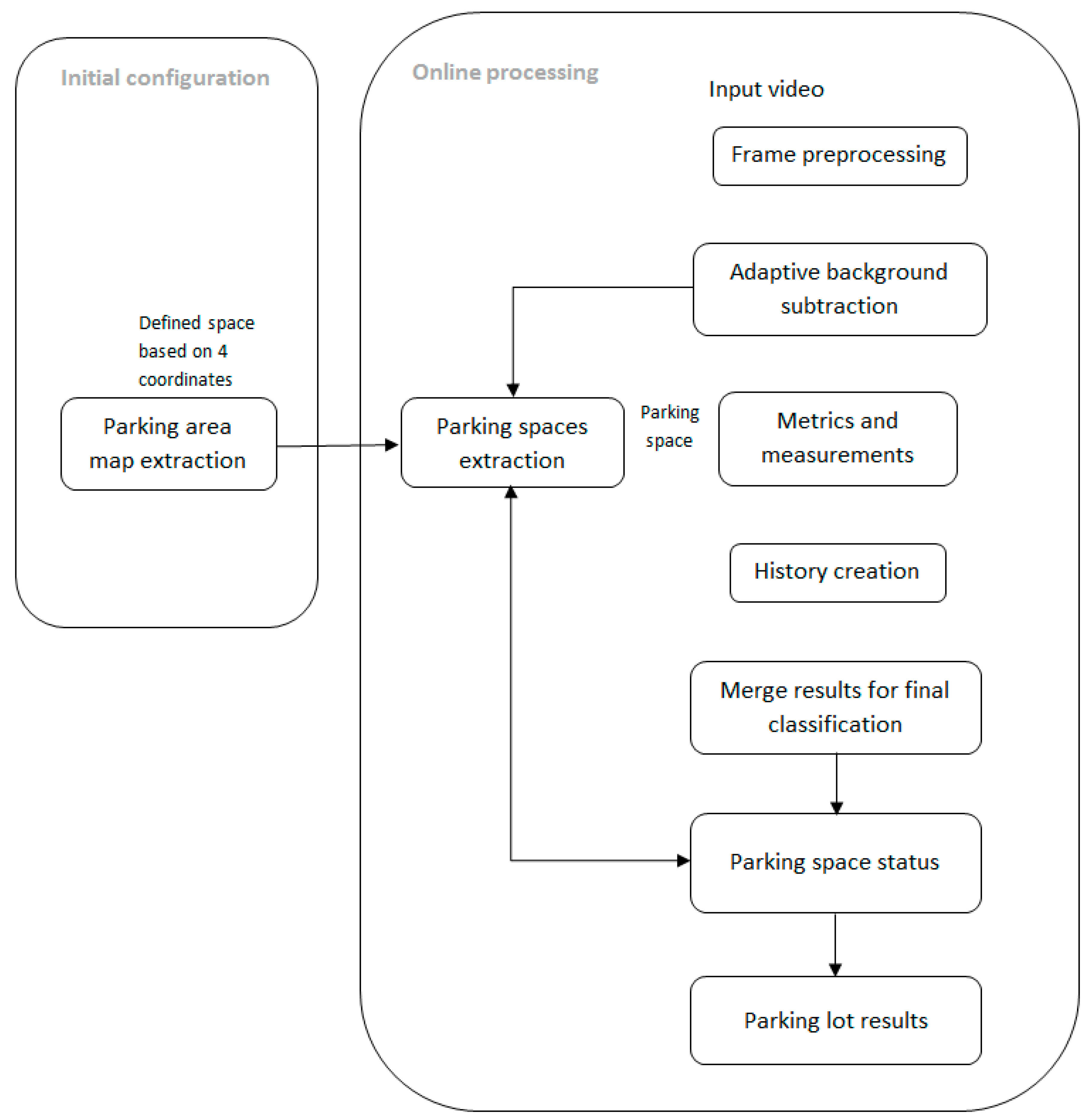
The proposed solution is divided into two steps: the initial configuration and the preprocessing chain, as shown in Figure 1. The initial configuration consists of a user-defined parking map based on a template image, managed offline and only once. The online preprocessing chain will then acquire the input video from the camera. Initially, the background is extracted, and, afterward, using the predefined map, each parking space is extracted and various history-based metrics and measurements are computed in order to determine the status of the parking space. Finally, the number of available and occupied parking spaces are determined.

2.1. Initial Configuration

In order to determine the available spaces in a parking lot (how many spaces are available and their localization), it is necessary to obtain information concerning the structure of the monitored parking area.

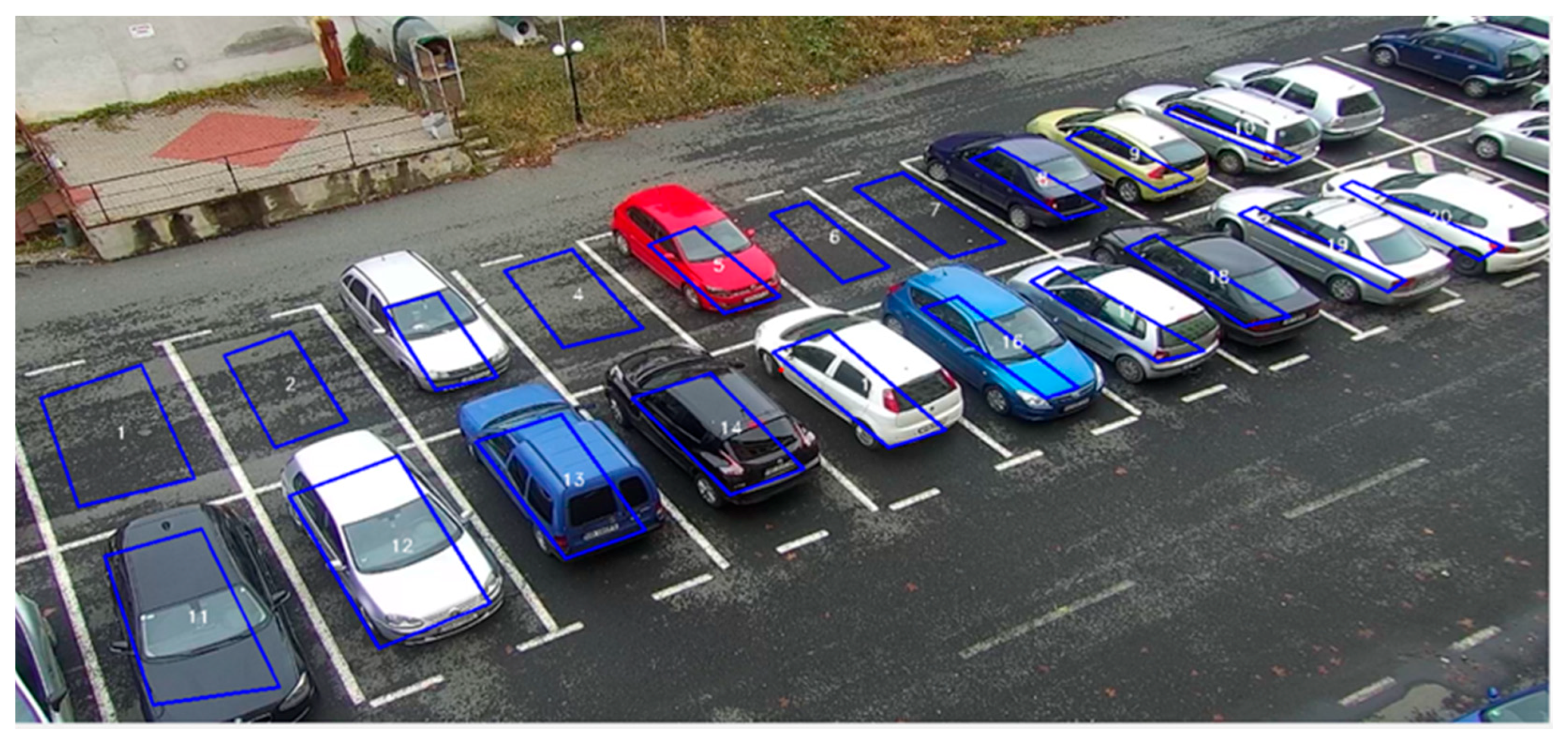
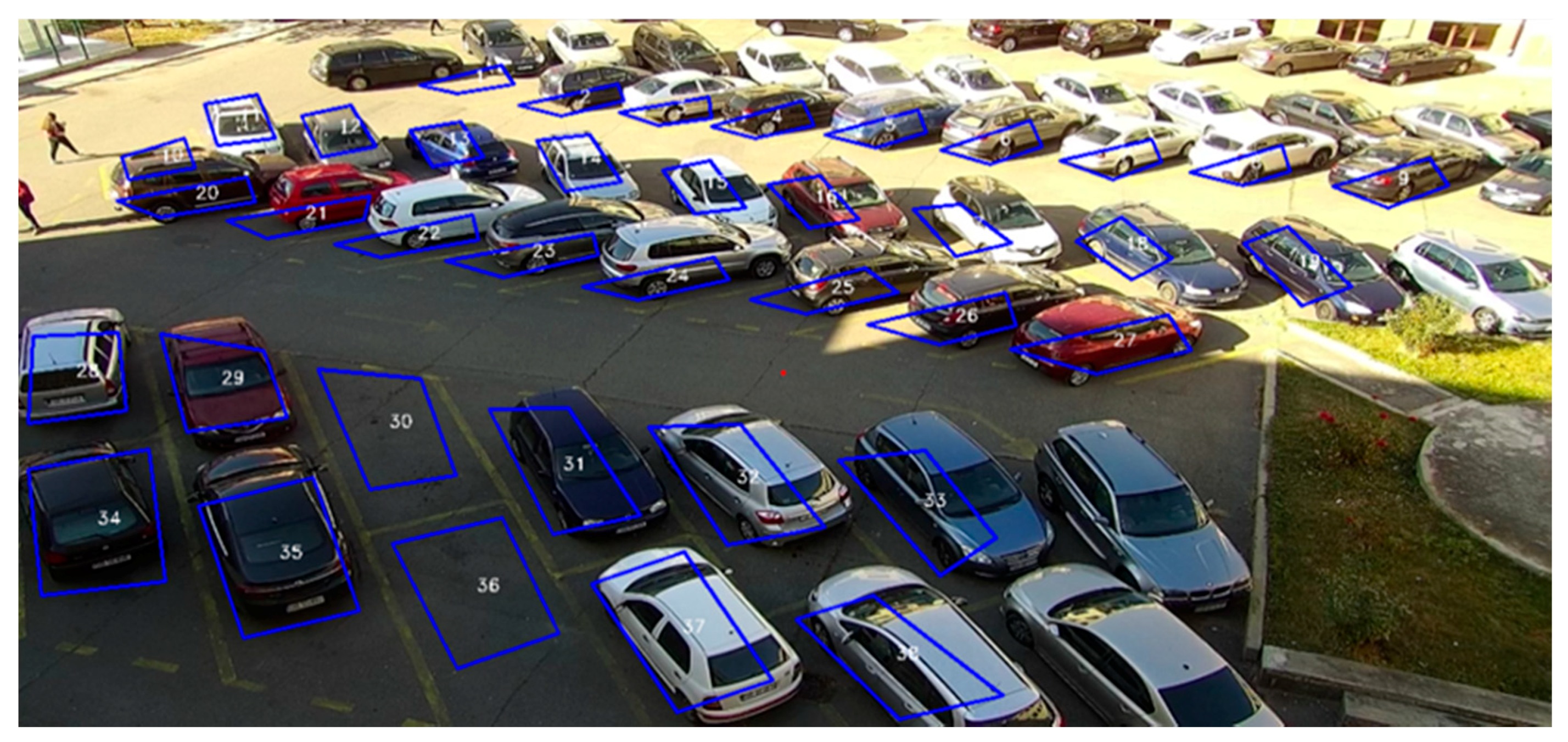
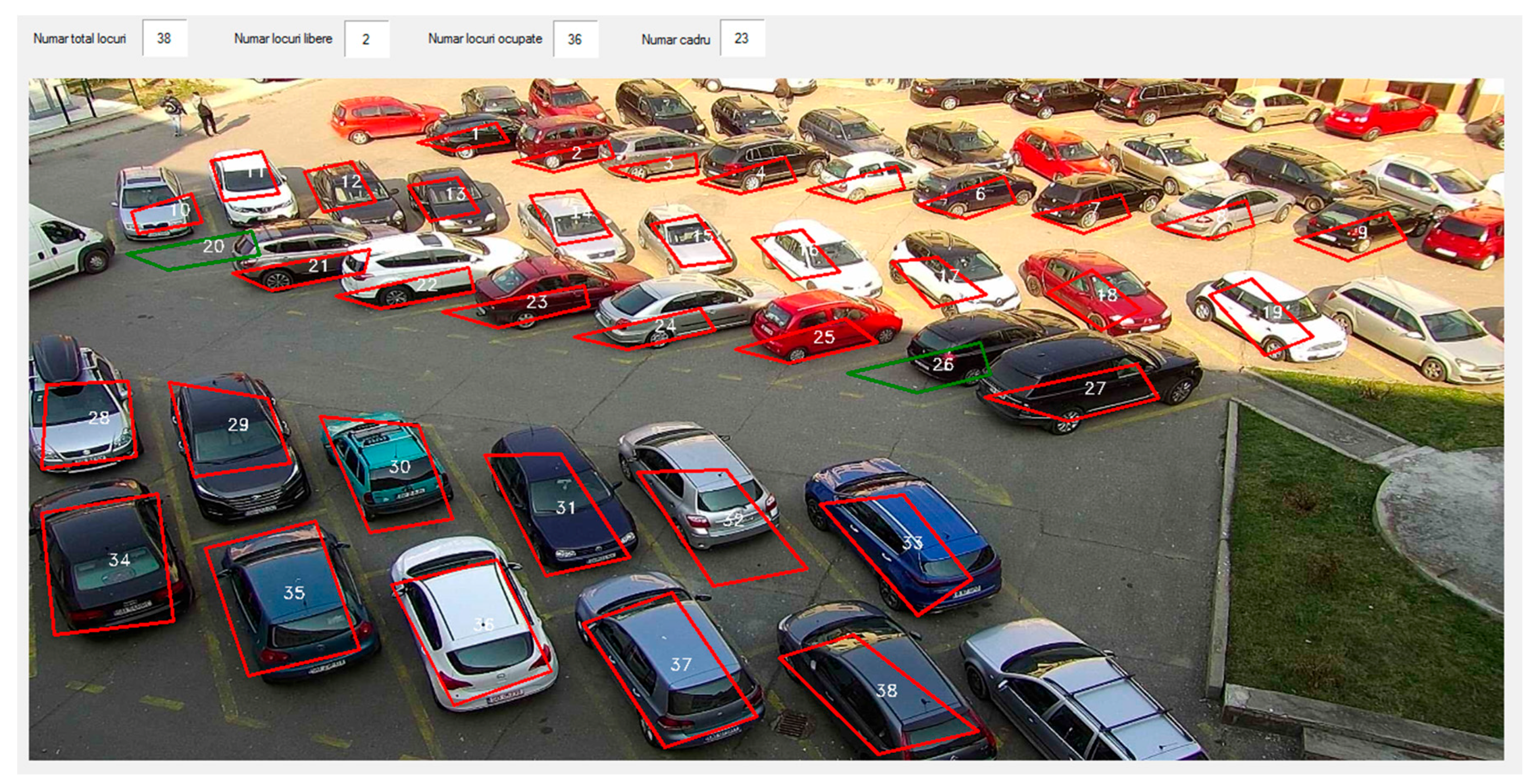
During this stage, a model for tracking the parking spaces on the pavement is provided. A graphic interface will be used for uploading an image with the observed parking area, and the user can trace the corners of each parking space. Using a pointer, four points for each parking space need to be marked. Once the provided points are saved, the system generates the map of the parking area which includes both the selected parking spaces, as well as their automatic numbering. This model is saved and will be reloaded for online use. Figure 2 and Figure 3 illustrate the maps generated in this research for two different parking areas.

2.2. The Image Processing Chain

During this stage, the main goal of the proposed algorithm resides in assigning a status to each parking space based on the extraction of several different image features from the map provided in the initial configuration.

2.2.1. Frame Preprocessing

Preprocessing is performed on the images acquired from the video camera, in order to remove noise as well as to smooth the edges. During tests on both benchmarks and online processing, we have noticed the necessity of preprocessing to improve both efficiency and algorithm results. We apply SmoothMedian (size) and SmoothBlur (ksize) to the original image of the type RGB. The median filter functionality is expressed by Equation (1).

$$\mathrm{median}\left\{{\mathrm{x}}_1,{ \mathrm{x}}_2, \dots ,{ \mathrm{x}}_{\mathrm{n}}\right\}= \{\begin{array}{c}{\mathrm{x}}_{\frac{\mathrm{n}+1}{2}} \mathrm{if} \mathrm{n} \mathrm{odd},\\ \frac{1}{2}{\mathrm{x}}_{\frac{\mathrm{n}}{2}}+\frac{1}{2}{\mathrm{x}}_{\frac{\mathrm{n}}{2}+1} \mathrm{if} \mathrm{n} \mathrm{even}.\end{array}$$

(1)

Function SmoothBlur (ksize) smoothes the image using the kernel:

$$\mathrm{K}=\frac{1}{\mathrm{ksize}.\mathrm{width}·\mathrm{ksize}.\mathrm{height}}\left[\begin{array}{c}1 1\dots 1\\ 1 1\dots 1\\ \dots \\ 1 1\dots 1\end{array}\right]$$

(2)

2.2.2. Adaptive Background Subtraction

Background subtraction is the first and fundamental step in many computer vision applications, such as traffic monitoring or parking lot occupancy. It is hard to produce a robust background model that works well under a vast variety of situations. A good background model should have the following features: accuracy in terms of form detection and reactivity to changes over time, flexibility under different lighting conditions, and efficiency for real-time delivery.

The mixture-of-Gaussians (MoG) background model is widely used in such applications, in order to segment moving foreground, due to its effectiveness in dealing with gradual lighting changes and repetitive motion. MoG is a parametric method employing statistics by using a Gaussian model for each pixel. Every Gaussian model maintains the mean and the variance of each pixel, with the assumption that each pixel value follows a Gaussian distribution. If considering the swaying of a tree or the flickering of a monitor, the MoG can handle those multi-model changes quite well [10]. Many improvements on Gaussian mixture model have been implemented like MOG2. An important feature of MOG2 is that it selects the appropriate number of Gaussian distributions for each pixel, providing better adaptability to varying scenes, due to illumination or other changes.

In this approach, the mixture of Gaussians algorithm (MOG2) was used for background subtraction, with the help of which two images were acquired: the background and the foreground. The background model is dynamically updated to compare each pixel with the corresponding distribution, leading to the foreground mask separated from the background. The foreground mask generated is a binary image, where foreground objects are white pixels. One or more objects can be detected in the foreground of a single image. The resulting background image is used as input for the next stage, the extraction of parking spaces.

The system involves the use of a Gaussian mixture model to adjust the probability density function (PDF) of each pixel X(x, y) and create the background model. The probability of observing the value of a pixel is defined as follows [10]:

$$\mathrm{P}\left({\mathrm{X}}_{\mathrm{t}}\right)= {{\displaystyle \sum }}_{\mathrm{i}=1}^{\mathrm{K}}{\mathsf{\omega }}_{\mathrm{i},\mathrm{t} }\mathrm{x} \mathsf{\eta }\left({\mathrm{X}}_{\mathrm{t}};{ \mathsf{\mu }}_{\mathrm{i},\mathrm{t}},{{\displaystyle \sum }}_{\mathrm{i},\mathrm{t}} \right)$$

(3)

with the values of a pixel at any time t, is known as its history [7]:

$$\left\{{\mathrm{X}}_1,\dots .,{ \mathrm{X}}_{\mathrm{t}}\right\}=\left\{\mathrm{I}\left({\mathrm{x}}_0,{\mathrm{y}}_0,\mathrm{i}\right) :1 \le \mathrm{i}\le \mathrm{t}\right\}$$

(4)

where K is the number of Gaussian distributions used to model each pixel, ω_i,t is the weight of the ${\mathrm{i}}^{\mathrm{th}}$ Gaussian at time t, µ_i,t is the Gaussian average of the ${\mathrm{i}}^{\mathrm{th}}$ Gaussian at time t, ${{\displaystyle \sum }}_{\mathrm{i},\mathrm{t}}$ is the covariance matrix of the ${\mathrm{i}}^{\mathrm{th}}$ Gaussian probability density function:

$$\mathsf{\eta }\left({\mathrm{X}}_{\mathrm{t}}, \mathsf{\mu },{\displaystyle \sum }\right)=\frac{1}{{\left(2\mathsf{\pi }\right)}^{\frac{\mathrm{n}}{2}}{\left|{\displaystyle \sum }\right|}^{\frac{1}{2}}}{\mathrm{e}}^{-\frac{1}{2}{\left({\mathrm{X}}_{\mathrm{t}}-{\mathsf{\mu }}_{\mathrm{t}}\right)}^{\mathrm{T}}{\displaystyle \sum }^{-1}\left({\mathrm{X}}_{\mathrm{t}}-{\mathsf{\mu }}_{\mathrm{t}}\right)}$$

(5)

Usually, the number of Gaussian distributions used to model each pixel is three or five. These Gaussians are correctly mixed due to the weight factor ω_i,t, which is altered (increased or decreased) for each Gaussian, based on how often the input pixel matches the Gaussian distribution.

The covariance matrix is defined as follows:

$${{\displaystyle \sum }}_{\mathrm{i},\mathrm{t}} ={ \mathsf{\sigma }}_{\mathrm{i},\mathrm{t}}^2\mathrm{I}$$

(6)

Once the parameters initialization is made, a first foreground detection can be made and then the parameters are updated. The K distribution are ordered based on the fitness value ${\mathsf{\omega }}_{\mathrm{k}}/{\mathsf{\sigma }}_{\mathrm{k}}$.

The Gaussian model will be updated by the following update equations [10]:

$${\mathsf{\mu }}_{\mathrm{t}}=\left(1-\mathsf{\rho }\right){\mathsf{\mu }}_{\mathrm{t}-1}+{\mathsf{\rho }\mathrm{X}}_{\mathrm{t}}$$

(7)

$${\mathsf{\sigma }}_{\mathrm{t}}^2=\left(1- \mathsf{\rho }\right){\mathsf{\sigma }}_{\mathrm{t}-1}^2+ \mathsf{\rho }{\left({\mathrm{X}}_{\mathrm{t}}-{ \mathsf{\mu }}_{\mathrm{t}}\right)}^{\mathrm{T}}\left({\mathrm{X}}_{\mathrm{t}}-{\mathsf{\mu }}_{\mathrm{t}}\right)$$

(8)

$${\mathsf{\omega }}_{\mathrm{t}}=\left(1- \mathsf{\alpha }\right){\mathsf{\omega }}_{\mathrm{t}-1}+ \mathsf{\alpha }$$

(9)

where

$$\mathsf{\rho }=\mathsf{\alpha }·\mathsf{\eta }\left({\mathrm{X}}_{\mathrm{t}+1},{ \mathsf{\mu }}_{\mathrm{i}},{{\displaystyle \sum }}_{\mathrm{i}} \right)$$

(10)

When the new frame at times t + 1 incomes, a match test is made for each pixel, where K is a constant threshold equal to 2.5. Thus, two cases can occur [11]:

Case 1: A match is found with one of the K Gaussians. In this case, if the Gaussian distribution is identified as a background one, the pixel is classified as background else the pixel is classified as foreground.

Case 2: No match is found with any of the K Gaussians. In this case, the pixel is classified as the foreground. At this step, a binary mask is obtained. Then, to make the next foreground detection, the parameters must be updated, using Equations (7)–(9).

The following processing steps will use the adaptive background image resulted from the background subtraction algorithm.

2.2.3. Extraction of the Area of Interest

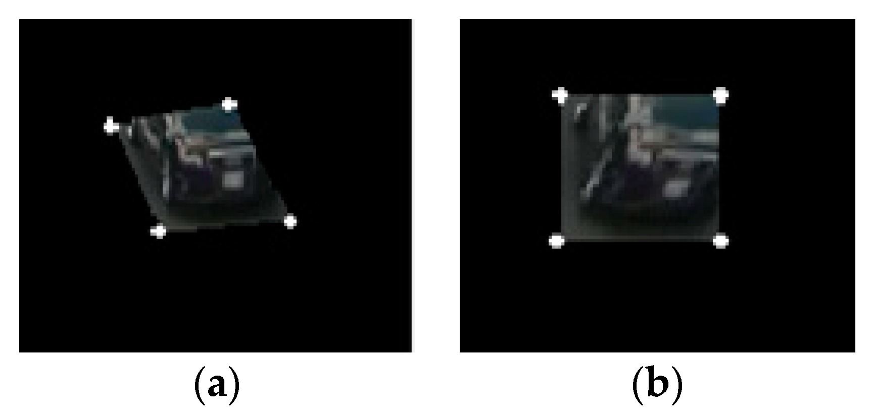
Based on the background image and the parking area map, each parking space is extracted and subjected to a perspective adjustment using the four marked points. From the resulted matrix, an image for each parking space is generated (see Figure 4).

2.2.4. Metrics and Measurements Used for Description of the Area of Interest

Based on the resulting images of the parking spaces, various methods and features are used for their detection into available and occupied places.

a. Histogram of Oriented Gradients (HOG)

Prior to applying the algorithm, the edges in the images must be detected and the image resized. The edge detection is done using the Canny algorithm, while the image is resized to 64 × 128 pixels. The histogram of oriented gradients (HOG) is a feature descriptor used to detect objects by counting the occurrences of gradient orientation in areas of interest. In the HOG feature descriptor, the distributions of the gradient orientation histogram are used as a feature, as follows:

• Sliding window dimension (winsize) is set to (64, 128). It defines the size of the descriptor.
• The size descriptor winSize is first divided into size cell cellSize (8, 8), and for each cell, a histogram of gradient direction or edge orientation is computed. Each pixel in the cell contributes to the histogram based on the gradient values [8].
• Adjacent cell groups are considered 2D regions called blocks, of size (16, 16). A Block uses blockSize.width · blockSize.height adjacent cells in order to estimate a normalized histogram out of the blockSize.width · blockSize.height cell histograms. Grouping the cells into a block is the basis for grouping and normalizing histograms. BlockStride can be used to arrange the blocks in an overlapping manner. BlockStride size is set to (8, 8).
• The histogram group constructs the block histogram. All normalized histograms estimated for each block are concatenated, defining the final descriptor vector.

An image gradient represents a directional change in the intensity or color of pixels and it is computed as partial derivatives (Equation (8)).

$$\Delta \mathrm{f}= \left[\frac{{\mathrm{g}}_{\mathrm{x}}}{{\mathrm{g}}_{\mathrm{y}}}\right]=\left[\frac{\frac{\partial \mathrm{f}}{\partial \mathrm{x}}}{\frac{\partial \mathrm{f}}{\partial \mathrm{y}}}\right]$$

(11)

where $\frac{\partial \mathrm{f}}{\partial \mathrm{x}}$ is the derivative with respect to x, $\frac{\partial \mathrm{f}}{\partial \mathrm{y}}$ is the derivative with respect to y.

The derivative of an image can be approximated by finite differences. To calculate $\frac{\partial \mathrm{f}}{\partial \mathrm{y}}$ one can apply a one-dimensional filter to the image by convolution:

$$\frac{\partial \mathrm{f}}{\partial \mathrm{y}}= \left[\begin{array}{c}-1\\ +1\end{array}\right]\ast \mathrm{A}$$

(12)

where * denotes the one-dimensional convolution operation.

The gradient direction can be computed as in Equation (13).

$$\mathsf{\theta }\left(\mathrm{x},\mathrm{y}\right)=\arctan \left(\begin{array}{c}\mathrm{dx}\\ \mathrm{dy}\end{array}\right)$$

(13)

while the magnitude is given by the following:

$$\mathrm{m}\left(\mathrm{x},\mathrm{y}\right)=\sqrt{{\mathrm{dx}}^2+{\mathrm{dy}}^2}$$

(14)

A histogram for each cell was created; with each cell pixel having one vote in the histogram. The interval of the histogram is incremented by a particular pixel is determined by the value of the gradient orientation. Dalal and Triggs [12] have found that it is enough to have nine histogram intervals, and if the gradient orientation takes values between 0 and 360 degrees, the position in the histogram is calculated by dividing the number by 40. In the polling process, each vote can be weighted with the magnitude of the gradient, with its square root or square magnitude.

To account for the light and contrast variations, the cells are organized into blocks and the normalization is performed for each block [13]. In [12], the authors indicate that the L2-norm is suitable for objects detection (Equation (2)).

$${\mathrm{v}}^{\prime }=\frac{\mathrm{v}}{\sqrt{{\left|\right|\mathrm{v}\left|\right|}_2^2+{\mathsf{ϵ}}^2}}$$

(15)

where v is a non-normalized vector containing all histograms obtained from the block and ε is a constant determined empirically with a low value. The HOG descriptor is the vector resulted from the normalized components of the histograms of each block cell.

The vector obtained from the HOG descriptor is used to compute an arithmetic mean. The values obtained are compared with the threshold defined as 0.03. If the value is bigger than this threshold, the parking space is tagged with 1 (occupied).

b. SIFT corner detector

Scale-invariant feature transform (SIFT) is a descriptor that is expressed as a multidimensional vector in $\mathrm{R}$ space and it features 128 dimensions. It can be considered a string of numbers assigned to a pixel, which reflects the influence of adjacent elements over the pixel in the image.

A SIFT vector is calculated as the weighted sum of normal values (intensities) over a gradient (pixel groups) considered adjacent to the analyzed pixel, where the weighting factor of the calculated sums is dependent on the distance from said pixel analyzed. It obtains superior results to the Harris corner detector and its features are highly consistent in terms of rotation, scaling, translation. The gray image is used to detect the key points based on the convolution with the kernel:

$$\mathrm{G}\left(\mathrm{x},\mathrm{y},\mathsf{\sigma }\right)=\frac{1}{2{\mathsf{\pi }\mathsf{\sigma }}^2}{\mathrm{e}}^{-\frac{{\mathrm{x}}^2+{\mathrm{y}}^2}{2{\mathsf{\sigma }}^2}}$$

(16)

where (x,y) is the location of the current pixel, $\mathsf{\sigma }$ is the standard deviation of Gaussian kernel. Computation of the differences convolutions at different scales σ will be performed.

$$\mathrm{D}\left(\mathrm{x},\mathrm{y},\mathsf{\sigma }\right)=\left(\mathrm{G}\left(\mathrm{x},\mathrm{y},\mathrm{k}\mathsf{\sigma }\right)-\mathrm{G}\left(\mathrm{x},\mathrm{y},\mathsf{\sigma }\right)\right) ·\mathrm{I}\left(\mathrm{x},\mathrm{y}\right)$$

(17)

$$\mathrm{D}\left(\mathrm{x},\mathrm{y},\mathsf{\sigma }\right)=\mathrm{L}\left(\mathrm{x},\mathrm{y},\mathrm{k}\mathsf{\sigma }\right)-\mathrm{L}\left(\mathrm{x},\mathrm{y},\mathsf{\sigma }\right)$$

(18)

where k is a natural number, I(x, y) represents the grayscale image.

This method extracts feature points, considered to be candidates in the extraction of “key points” used in the description of the image. For each point, the gradient magnitude and orientation will be computed using the following formulas:

$$\mathrm{m}\left(\mathrm{x},\mathrm{y}\right)=\sqrt{{\left(\mathrm{L}\left(\mathrm{x}+1,\mathrm{y}\right)-\mathrm{L}\left(\mathrm{x}-1,\mathrm{y}\right)\right)}^2+{\left(\mathrm{L}\left(\mathrm{x},\mathrm{y}+1\right)-\mathrm{L}\left(\mathrm{x},\mathrm{y}-1\right)\right)}^2}$$

(19)

$$\mathsf{\theta }\left(x,y\right)=ta{b}^{-1}\left[\frac{L\left(x,y+1\right)-L\left(x,y-1\right)}{L\left(x+1,y\right)-L\left(x-1,y\right)}\right]$$

(20)

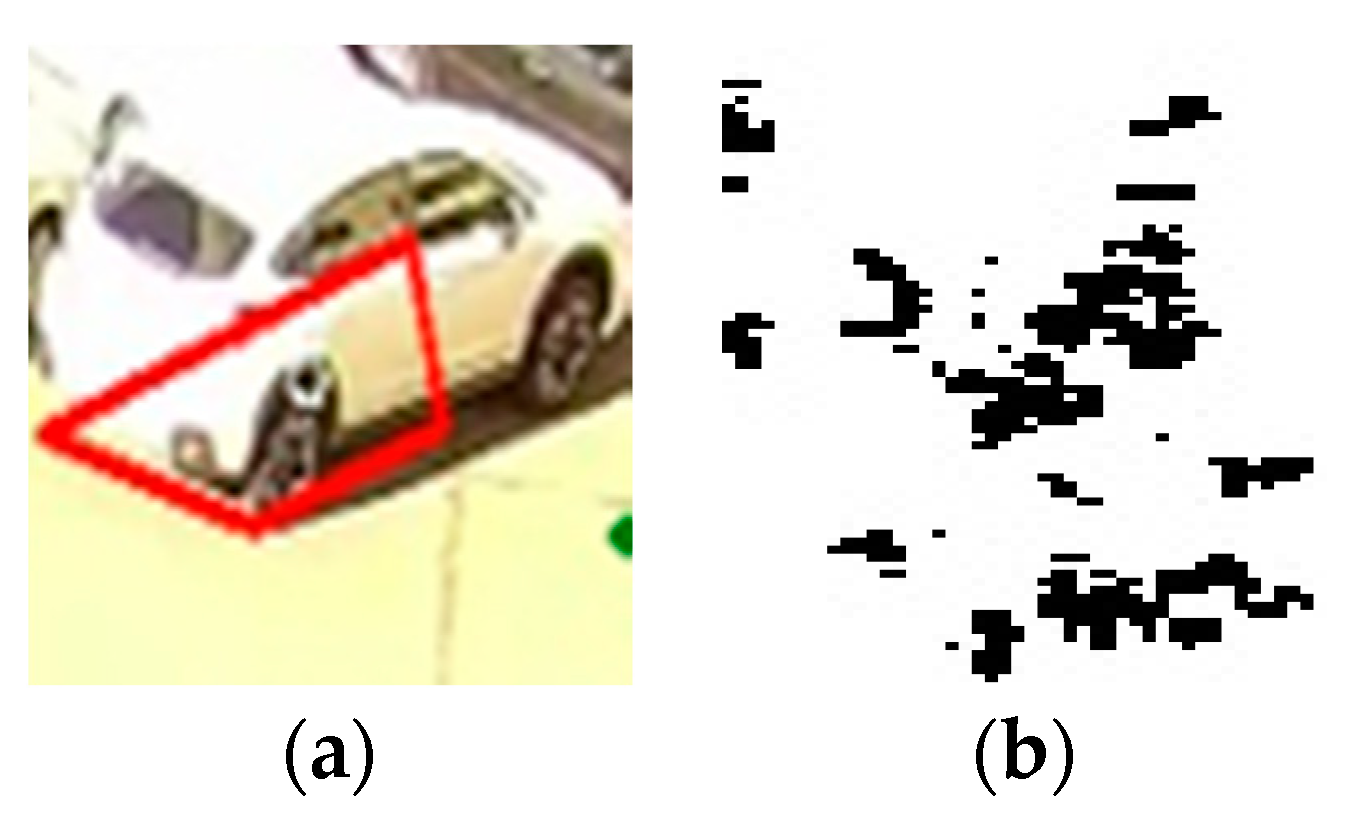
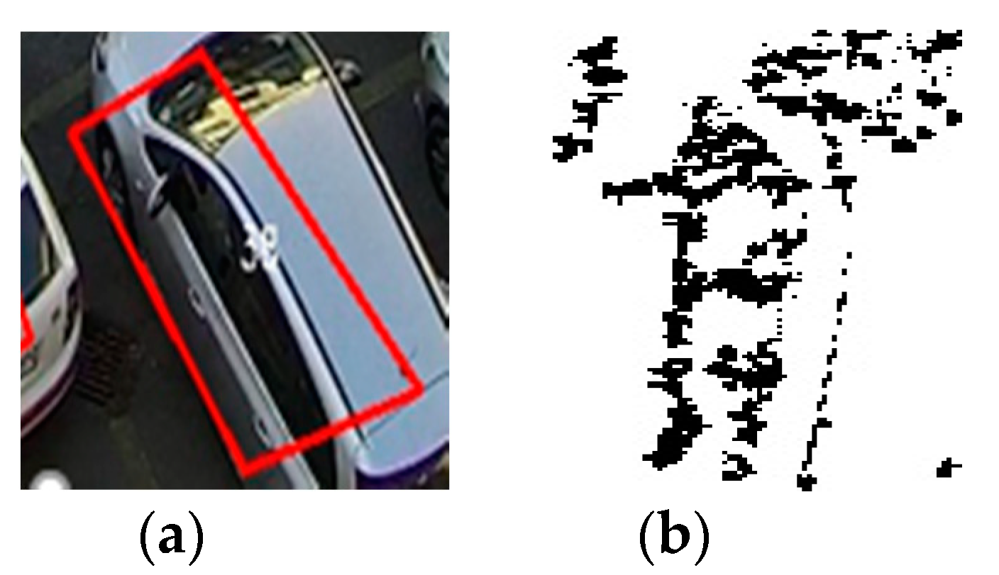
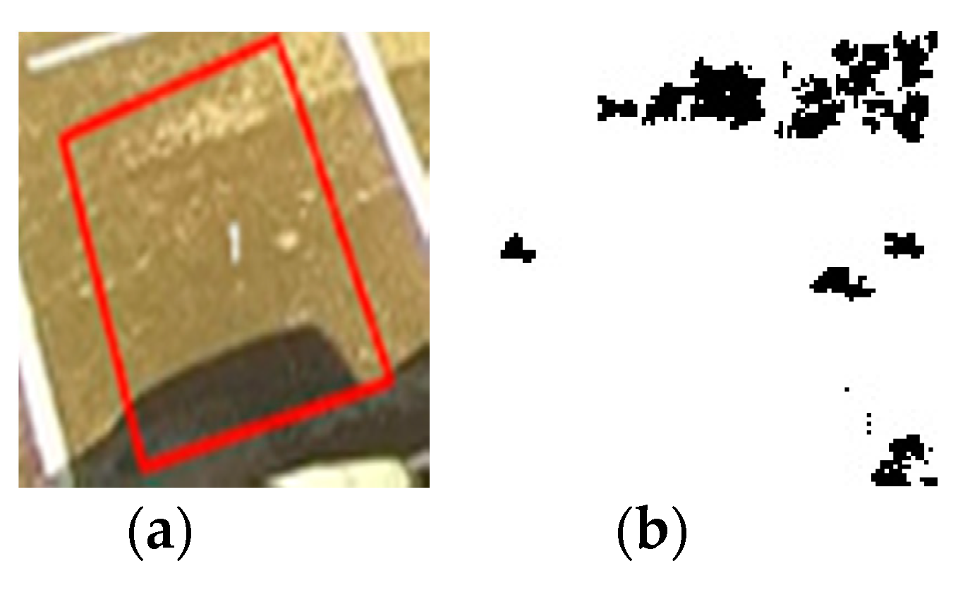
An orientation histogram will be created and the maximum values will be retained, together with points containing at least 80% of the maximum value found (eliminating thus over 95% of the points extracted in the previous process). After obtaining the extremes, the points with low contrast and less outlined edges will be eliminated. The remaining points are the points of interest in the image as one can see from Figure 5, Figure 6 and Figure 7.

The number of the points of interest from the SIFT corner detector is compared with threshold = 7 and if the value is bigger than the threshold, then status = 1 (occupied space); otherwise, status = 0 (available space).

The corner detector is combined with the HOG in order to obtain more accurate results.

$$\mathrm{status}=\{\begin{array}{c}1 \mathrm{as} \mathrm{occupied} \mathrm{space}, \mathrm{if} \mathrm{results} \mathrm{from} \mathrm{SIFT} \mathrm{and} \mathrm{from} \mathrm{HOG} \mathrm{are} 1\\ 0 \mathrm{as} \mathrm{available} \mathrm{space}, \mathrm{if} \mathrm{results} \mathrm{from} \mathrm{SIFT} \mathrm{and} \mathrm{from} \mathrm{HOG} \mathrm{are} 0\\ \mathrm{result} \mathrm{from} \mathrm{HOG}, \mathrm{if} \mathrm{results} \mathrm{from} \mathrm{SIFT} \mathrm{and} \mathrm{from} \mathrm{HOG} \mathrm{are} \mathrm{different}\end{array}$$

The parking space status is labeled as occupied if the result of the detection methods employed is mostly “1”, and the parking space status is labeled as available if the result is mostly “0”. In case of various background interferences such as shade, sun, or camouflage, the results are erroneous. In the case of camouflage, no corners are detected for the occupied spaces, and they are labeled as available. In the case of shade or sun, corners are detected in the available spaces, and they are labeled as occupied. To eliminate these background issues, we will add some metrics discussed in the next section.

c. Metrics on Color Spaces YUV, HSV, and YCrCb

YUV defines a color space where U is the color difference between red and blue, and V is the color difference between green and magenta. Y is the weighted values of red, green and blue [14], and represents the luminance component. U and V stand for the color components. Chrominance is defined as the difference between a color and a shade of gray with the same luminance.

$$\mathrm{Y}=0.299·\mathrm{red}+0.587·\mathrm{green}+0.114·\mathrm{blue}$$

(21)

$$\mathrm{U}=\mathrm{blue}-\mathrm{Y}$$

(22)

$$\mathrm{V}=\mathrm{red}-\mathrm{Y}$$

(23)

The HSV color space is a uniform one and is a trade-off between a perceptual relevance and computation speed, while in our context, it has been proved to detect the shade more accurately. The theoretical basis for removing shade is that the hues of brightness and saturation are darker than those in the background, but the color remains unchanged when the image is converted to the HSV color space [15].

YCbCr is a color model which includes a luminance component (Y) and two chrominance components (Cb and Cr), where Cb is the blue chrominance component, and Cr is the red chrominance component.

$$\mathrm{Y}=0.2126·\mathrm{red}+0.7152·\mathrm{green}+0.0722·\mathrm{blue}$$

(24)

$$\mathrm{Cb}=0.5389·\left(\mathrm{blue}-\mathrm{Y}\right)$$

(25)

$$\mathrm{Cr}=0.6350· \left(\mathrm{red}-\mathrm{Y}\right)$$

(26)

The measurement used for these metrics is the standard deviation. The vectors obtained from the three color spaces, the standard deviation is calculated on the following channels:

• YUV: standard deviation on channel V;
• HSV: standard deviation on channel S;
• YCbCr: standard deviation on channel Cb;

The values obtained from measurements of metrics are compared with thresholds defined in the system. The thresholds are 1.4 for V component from YUV, 9 for S component from HSV and 1.1 for Cb component from YCbCr. If the value is bigger than the threshold, the parking space is tagged with 1 (occupied). The values of 1 (occupied) and 0 (free) from these measurements are counted and the state of the parking space is set in history in Section 2.2.5. If the predominant is 1, the parking space is occupied, and otherwise is free.

After combining the YUV, HSV, and YCbCr color spaces with descriptor HOG and SIFT, the results improved significantly. The standard deviations on the three transformations were included in the generated history.

2.2.5. Feature Tracking

The standard deviation values for the three channels V (devSYUV), S (devSHSV), Cb (devSYCrCb) of the color spaces YUV, HSV, YcbCr, the number of corners (noSIFT), and the HOG descriptor mean (meanHOG) were used to create a history, based on predefined thresholds mentioned in Section 2.2.4. This history tracks the availability of parking spaces.

Each value from metrics and measurements compares with a default threshold. Based on this comparison, the values of 1 (statusOccupied) and 0 (statusAvailable) are counted, and the status is determined by the predominant value.

   Function SetStatus (indexParkingLot)
   if meanHOG[indexParkingLot] > 0.03 then statusOccupied++;
   else statusAvailable++;
   end if
   if noSIFT[indexParkingLot] >= 7 then statusOccupied++;
   else statusAvailable++;
   end if
   if devSYUV[indexParkingLot] > 1.4 then statusOccupied++;
   else statusAvailable++;
   end if
   if (devSHSV[indexParkingLot] > 9) then statusOccupied++;
   else statusAvailable++;
   end if
   if (devSYCrCb[indexParkingLot] > 1.1) then statusOccupied++;
   else statusAvailable++;
   end if
   if (statusAvailable > statusAvailable) then status = 0
   else status = 1
   end if
   EndStatus

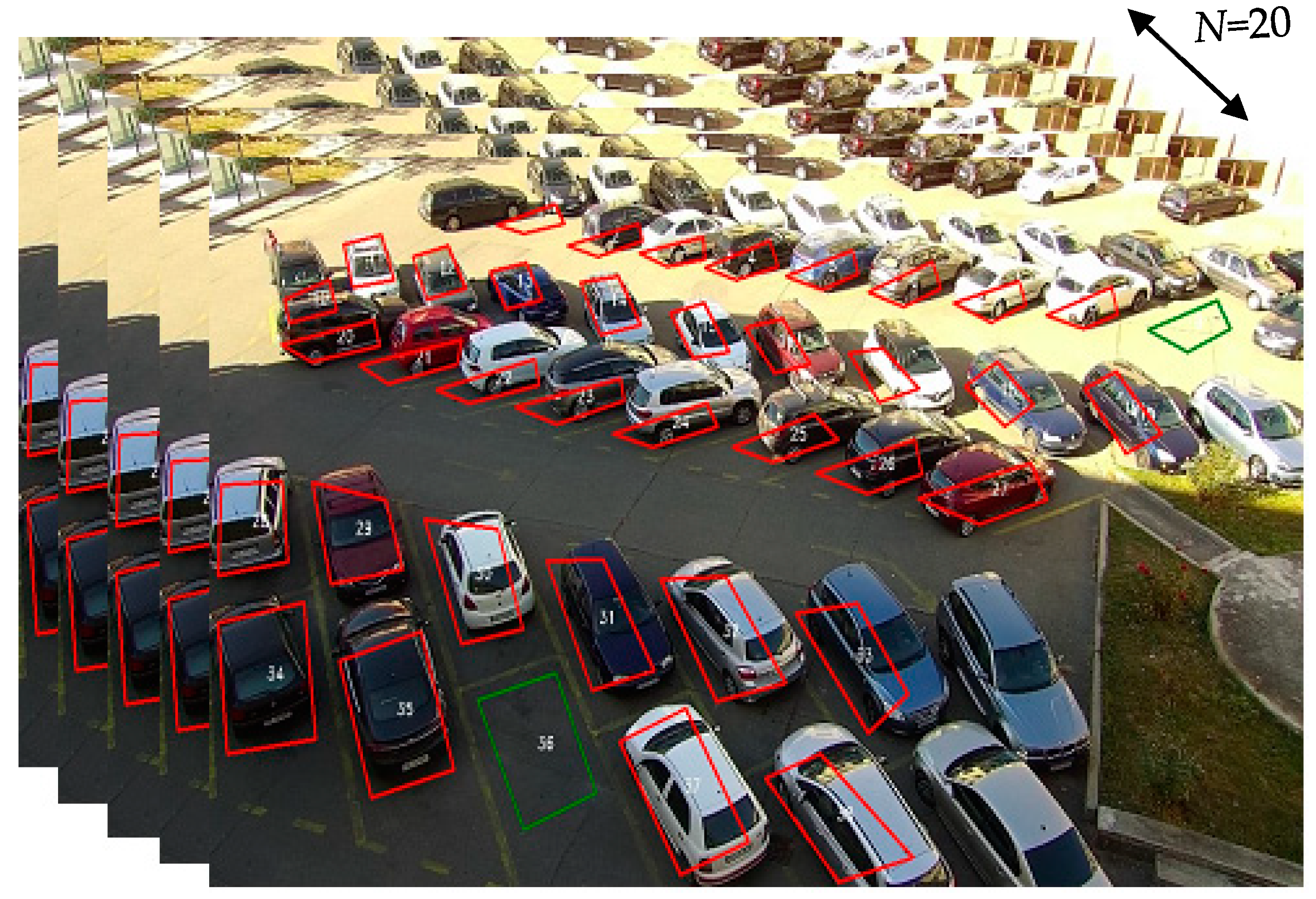
For more accurate results, was have created a history of 20 frames (Figure 8), that memorizes the status of each parking space, obtained from measured metrics and measurement results. With each new frame, it is tested if the number of frames originally set has been reached. If yes, then adding the status to the list produces the effect of a “sliding window”, which requires the elimination of the first value of the buffer and the addition of the new value in the list, according to the FIFO principle. Thus, this technique allows for the last changes to each parking space to be retained in order to determine the status. Over time, this process helps stabilize changes in the background, such as the gradual change from day to night, different weather conditions.

for parkingSpace=0:totalNumberParkingLot
	if(sizeOfBuffer < 20)
		Status = SetStatus(parkingSpace)
		Add status in buffer
else
		SlidingWindow
		Status = SetStatus(parkingSpace)
		Add status in buffer
	end if
	if predominat is 1 in buffer StatusParkingSpace = 1
	else StatusParkingSpace = 0
	end if
end for

2.2.6. Decision Process on Area of Interest

Based on the labeled status of each parking space obtained in Section 2.2.5, the total number of available and occupied spaces in a specific parking lot is recognized. The results are illustrated in Figure 9 and Figure 10.

3. Results of the Proposed Method

3.1. Benchmarks and Metrics Used for Validation

The images used for testing purposes show two parking lots with 36 and 20 parking spaces, respectively, and were taken from fixed cameras. For this reason, the parking lot map is extracted only once, at system initialization. In view of an evaluation and without any benchmark available, we have created and manually annotated two of them, taken from the available cameras. Benchmark 1 has a total number of 90,984 frames, while the benchmark 2 was acquired with 121,400 frames, both at full HD resolution.

The combination of the five methods used is the only one that has produced encouraging results in a good number of cases, but in the case of camouflage, cars overlapping the limits of a parking space, and under certain weather conditions (sun and shade), the assigned labels were wrong. System performance varies depending on meteorological conditions. However, accuracy is over 90%, making the system quite robust. The best performances are achieved in the absence of direct sunlight, with no shadows on the parking spaces.

For assessing the rate of parking spaces detection, the tests were performed in different moments, for each camera. One can find below the results from different benchmarks with the total number of frames.

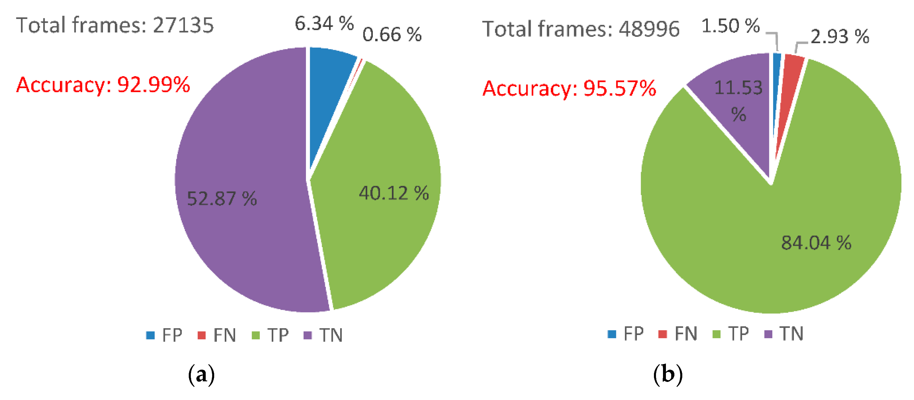
In order to evaluate the system performance, the following rates were calculated: false positive (FP), false negative (FN), true positive (TP), true negative (TN), and accuracy (ACC).

$$\mathrm{ACC}=\frac{\mathrm{TP}+\mathrm{TN} }{\mathrm{FP}+\mathrm{FN}+\mathrm{TP}+\mathrm{TN}}$$

(27)

where FP is the total number of available parking spaces labeled as occupied, FN is the total number for occupied parking spaced labeled as available, TP is the total number of available spaces correctly labeled, and TN the total number of occupied spaces correctly labeled.

3.2. Results

The results from

Table 1. Benchmark results using the combined methods of HOG, SIFT, color spaces YUV, HSV and YCrCb.

Benchmark	No. of Frames	Algorithms	FP (%)	FN (%)	TP (%)	TN (%)	Accuracy (%)
1	90,984	HOG, SIFT	36.7216	0	2.3637	60.9146	63.2783
		HOG, SIFT, YUV, HSV, YCrCb	5.0914	0	47.4542	47.4542	93.3902
2	121,400	HOG, SIFT	18.6388	5.2719	45.4698	30.6193	82.0846
		HOG, SIFT, YUV, HSV, YCrCb	3.3694	2.6306	19.9672	74.0327	93.0354

were obtained in unfavorable conditions, from a rainy/cloudy day benchmark, with wet spots in the parking spaces. It shows that the accuracy rate is better using a combination of the five metrics, as opposed to using only the HOG descriptor together with the SIFT corner detector.

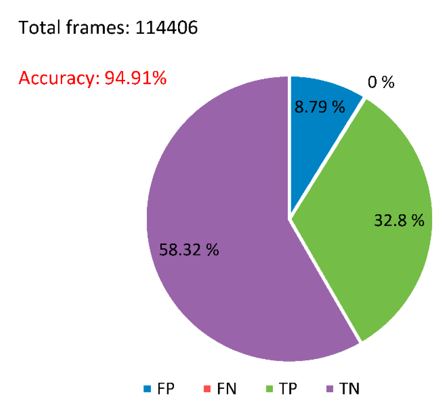
Using the proposed algorithm, fraction results are illustrated in Figure 11, obtaining an accuracy of 94.91%. This benchmark was used for tests over one day, after the rain, which led to wet spots on the asphalt, with periods of sun and shade.

Using the algorithms mentioned above for a different benchmark let to the results illustrated in Figure 12. The benchmark was tested on a sunny day. The tests show an accuracy of 96.60%, which reveals a very good detection rate.

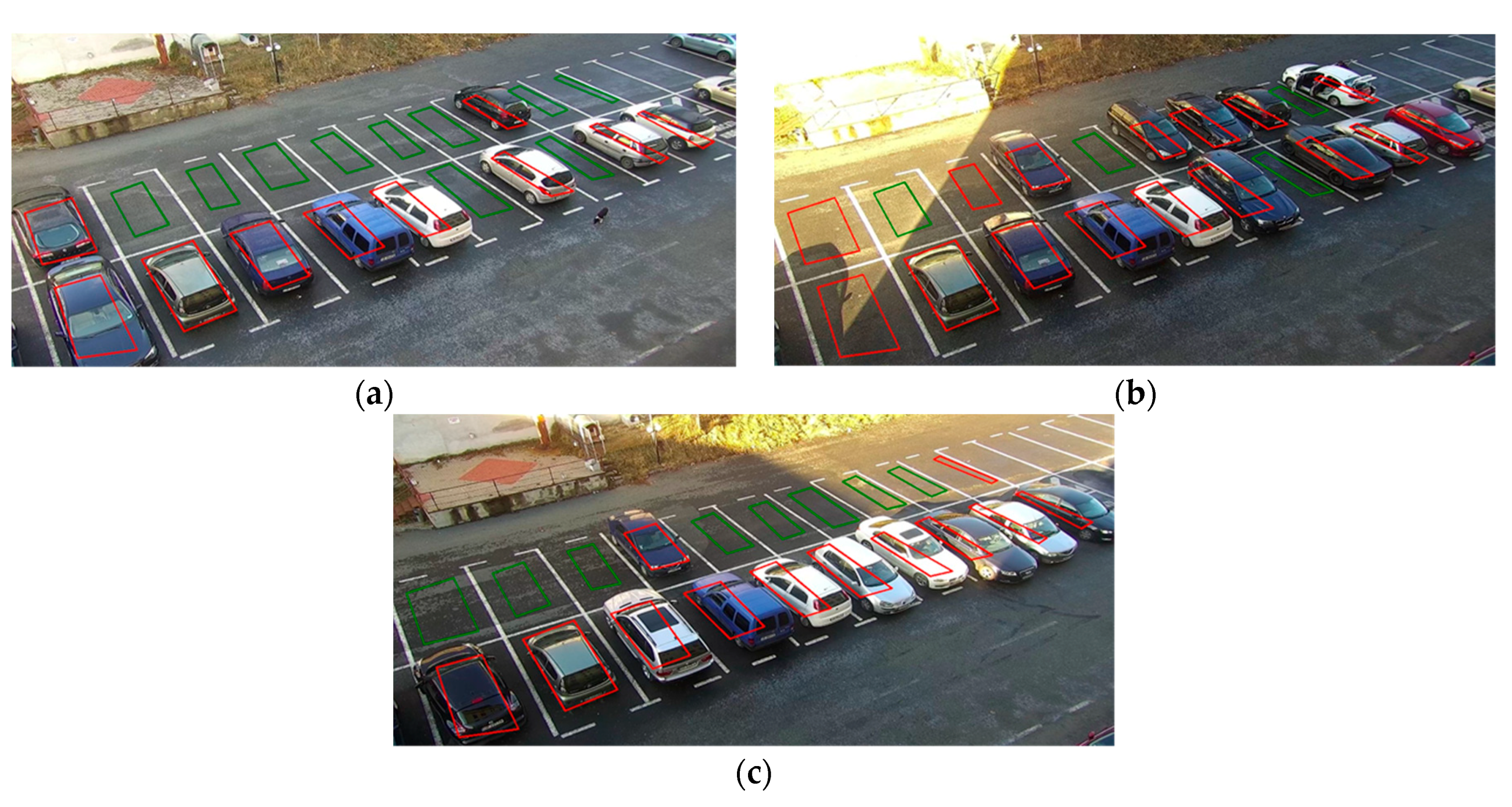
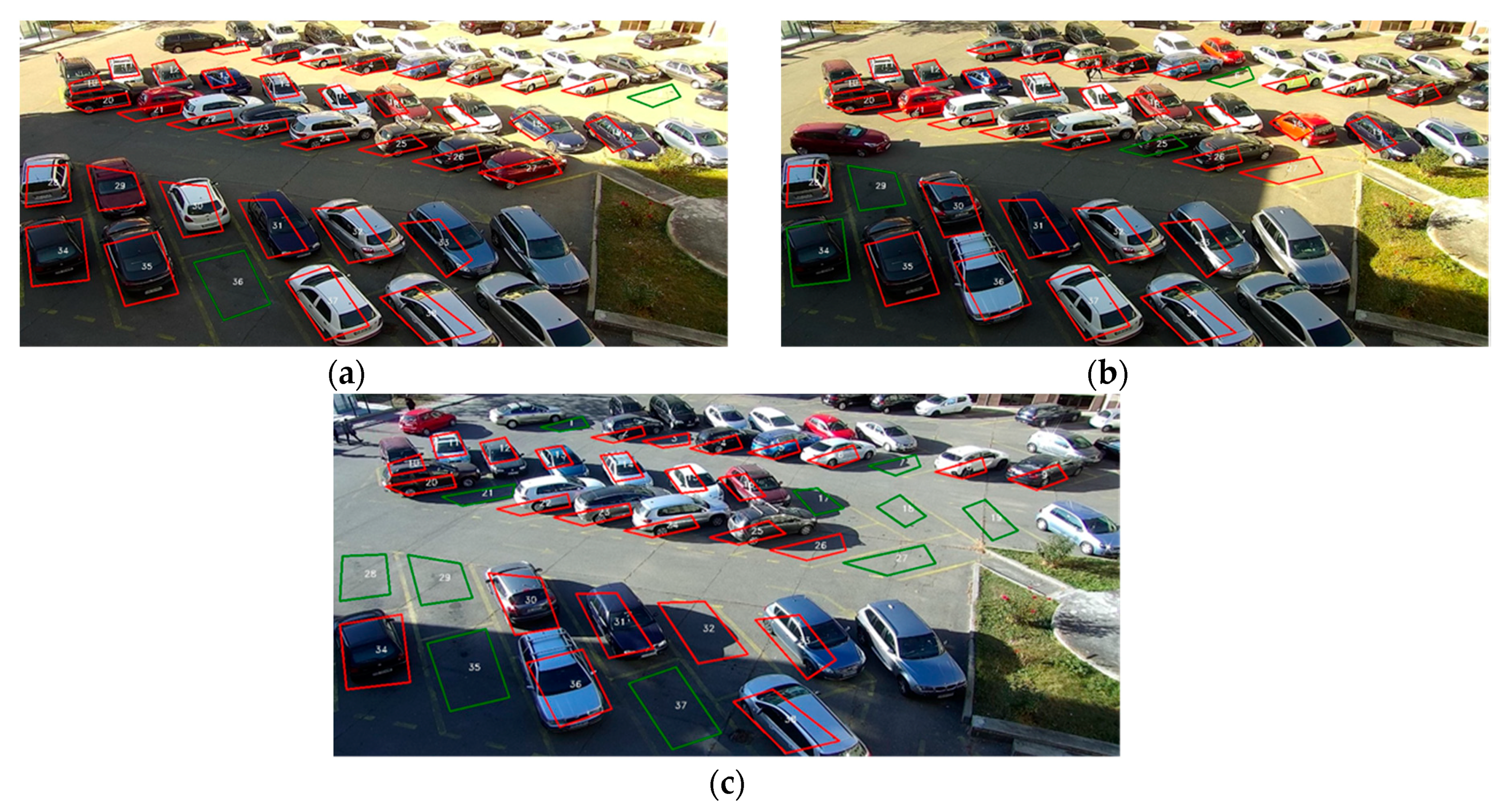
The images in Figure 13 and Figure 14 taken from cameras on a sunny day show that in direct sunlight, the results were reliable and the parking spaces were correctly labeled. Once shadows appeared, the available parking spaces affected were wrongly labeled at the beginning of history-based detection.

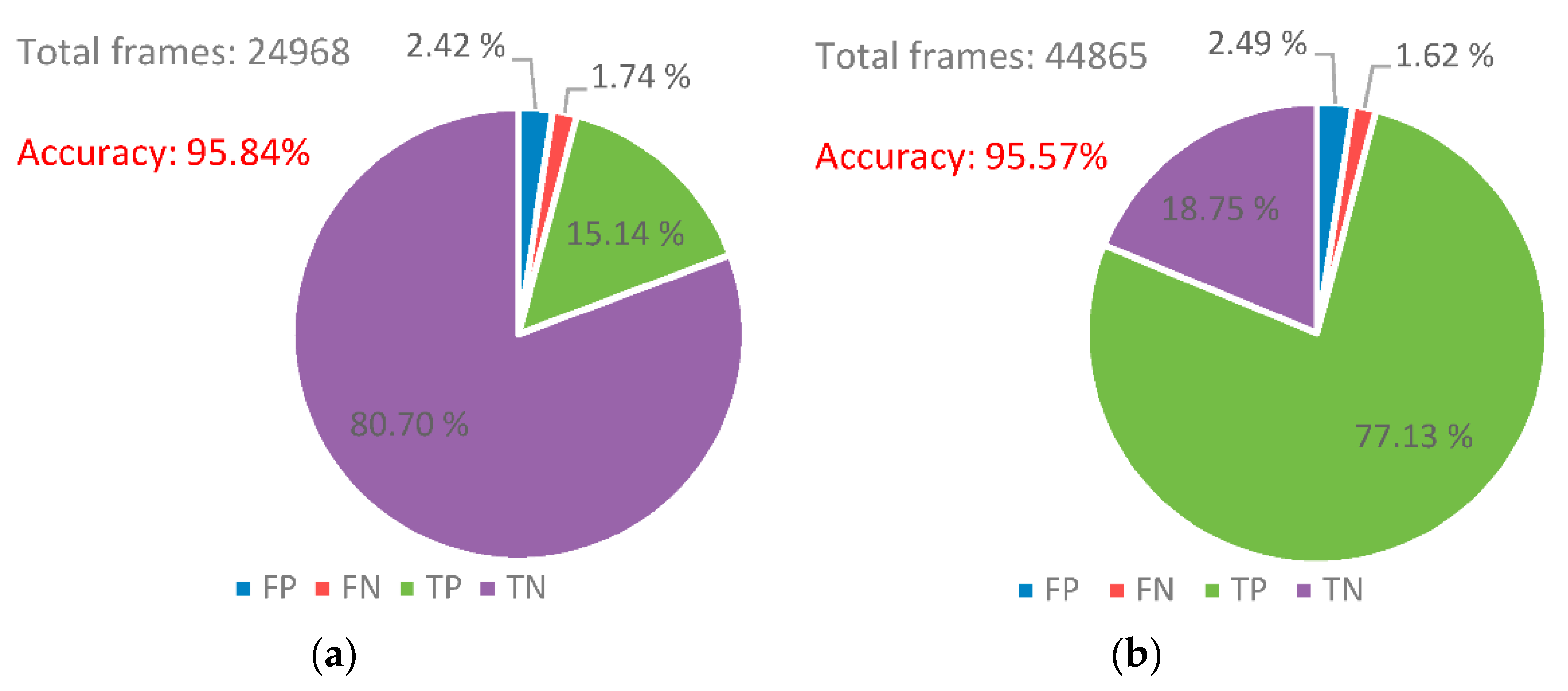
The benchmarks 1 and 2 have been annotated and tested over a 24-h period. In order to present the robustness of the proposed system, we have split each of them into the two periods of the day. The results presented in Figure 15 and Figure 16 show the accuracy between day and night, which has mostly the same values in detecting the parking spots, even if night time images are corrupted with camera noise.

4. Conclusions

In this paper, a video detection system for parking lot occupancy has been described. Compared to other methods, the system uses a single camera sensor for the detection of multiple parking spaces occupancy. Results achieved using the two parking lot installed cameras, have an accuracy rate of over 93%. In order to exploit adaptive background, a mixture of Gaussian model was used. The background is processed using the HOG descriptor, the SIFT corner detector, and the HSV, YUV, YCbCr color spaces to solve various detection issues. These combined algorithms improve the accuracy of the parking lot occupancy detection.

The applied algorithms have solved some of the background issues caused by the meteorological conditions, resulting in a high accuracy rate over a long period of time. The results with lower accuracy rate were due to unsolved issues, such as shade and camouflage, since the shade was identified as an object. However, over a long enough period of time, where there are intervals with different illumination conditions, the accuracy rate was over 93%.

Due to the straightforwardness and robustness of the proposed system, a commercial implementation is foreseen. IoT technology and Smart City applications, the duality of the proposed method, as security surveillance and also feature extraction for parking space detection, have substantial industrial potential.

References

- Masmoudi, I.; Wali, A.; Alimi, A.M. Parking spaces modelling for inter spaces occlusion handling. In Proceedings of the 22nd International Conference in Central Europe on Computer Graphics Visualization and Computer Vision, Plzen, Czech Republic, 2–5 June 2014. [Google Scholar]
- Bibi, N.; Majid, M.N.; Dawood, H.; Guo, P. Automatic parking space detection system. In Proceedings of the 2017 2nd International Conference on Multimedia and Image Processing (ICMIP), Wuhan, China, 17–19 March 2017; pp. 11–15. [Google Scholar]
- Wu, Q.; Zhang, Y. Parking Lots Space Detection; Technical Report; Carnegie Mellon University: Pittsburgh, PA, USA, 2006. [Google Scholar]
- Cazamias, J.; Marek, M. Parking Space Classification Using Convolutional Neural Networks; Technical Report; Stanford University: Stanford, CA, USA, 2016; Available online: http://cs231n.stanford.edu/reports/2016/pdfs/280_Report.pdf (accessed on 2 November 2018).
- Delibaltov, D.; Wu, W.; Loce, R.P.; Bernal, E.A. Parking lot occupancy determination from lamp-post camera images. In Proceedings of the 16th International IEEE Conference on Intelligent Transportation Systems (ITSC 2013), The Hague, The Netherlands, 6–9 October 2013; pp. 2387–2392. [Google Scholar]
- Yusnita, R.; Norbaya, F.; Basharuddin, N. Intelligent parking space detection system based on image processing. Int. J. Innov. Manag. Technol. 2012, 3, 232–235. [Google Scholar]
- George, T.S.H.; Yung, P.T.; Chun, H.W.; Wai, H.W.; King, L.C. A Computer Vision-Based Roadside Occupation Surveillance System for Intelligent Transport in Smart Cities. Sensors 2019, 19, 1796. [Google Scholar] [Green Version]
- Giuseppe, A.; Fabio, C.; Fabrizio, F.; Claudio, G.; Carlo, M.; Claudio, V. Deep Learning for Decentralized Parking Lot Occupancy Detection. Expert Syst. Appl. 2017, 72, 327–334. [Google Scholar]
- Mehmet, S.K.; Aline, C.V.; Luigi, I.; Daniel, K.; Gregory, M.; Jean, P.V. A Smart Parking Lot Management System for Scheduling the Recharging of Electric Vehicles. IEEE Trans. Smart Grid 2015, 6, 2942–2953. [Google Scholar]
- Wang, X.; Sun, J.; Peng, H.-Y. Foreground Object Detecting Algorithm based on Mixture of Gaussian and Kalman Filter in Video Surveillance. J. Comput. 2013, 8, 693–700. [Google Scholar]
- Bouwmans, T.; El Baf, F.; Vachon, B. Background Modeling using Mixture of Gaussians for Foreground Detection—A Survey. Recent Pat. Comput. Sci. 2008, 1, 219–237. [Google Scholar] [CrossRef]
- Dalal, N.; Triggs, B. Histograms of oriented gradients for human detection. In Proceedings of the International Conference on Computer Vision & Pattern Recognition (CVPR’05), Computer Society, San Diego, CA, USA, 20–25 June 2005; pp. 886–893. [Google Scholar]
- Prates, R.F.; Cámara-Chávez, G.; Schwartz, W.R.; Menotti, D. Brazilian License Plate Detection Using Histogram of Oriented Gradients and Sliding Windows. Int. J. Comput. Sci. Inf. Technol. 2013, 5, 39–52. [Google Scholar]
- Koschan, A.; Abidi, M. Digital Color Image Processing; John Wiley Sons: Hoboken, NJ, USA, 2008. [Google Scholar]
- Zhang, X.; Liu, K.; Wang, X.; Yu, C.; Zhang, T. Moving shadow removal algorithm based on HSV color space. Indones. J. Electr. Eng. 2014, 12, 2769–2775. [Google Scholar] [CrossRef]
Figure 1.
Parking lot occupancy system processing diagram.
Figure 2.
Defined parking area map on benchmark 1.
Figure 3.
Defined parking area map on benchmark 2.
Figure 4.
The image of the parking space: (a) before the adjustment; (b) after the perspective adjustment.
Figure 5.
The image of (a) sunny parking space; (b) the result of SIFT corner detector.
Figure 6.
The image of (a) occupied parking space); (b) the result of SIFT corner detector.
Figure 7.
The image of (a) available sunny parking space; (b) the result of SIFT corner detector.
Figure 8.
Frame history on 20 consecutive frames.
Figure 9.
A result sample from benchmark 1.
Figure 10.
A result sample from benchmark 2.
Figure 11.
Results on benchmark 1.
Figure 12.
Results on benchmark 2.
Figure 13.
Detection of parking lot 1 availability: (a) the before direct sunlight; (b) with direct sunlight; (c) at the end of the day.
Figure 14.
Detection of parking lot 2 availability: (a) the before direct sunlight; (b) with direct sunlight; (c) at the end of the day.
Figure 15.
Results on benchmark 1 over: (a) day, (b) night.
Figure 16.
Results on benchmark 2 over: (a) day, (b) night.