Unsteady Multi-Element Time Series Analysis and Prediction Based on Spatial-Temporal Attention and Error Forecast Fusion

School of Computer Engineering and Science, Shanghai University, Shanghai 200444, China
*
Author to whom correspondence should be addressed.
Future Internet 2020, 12(2), 34; https://0-doi-org.brum.beds.ac.uk/10.3390/fi12020034
Submission received: 24 December 2019
/
Revised: 16 January 2020
/
Accepted: 8 February 2020
/
Published: 13 February 2020
Abstract
:Harmful algal blooms (HABs) often cause great harm to fishery production and the safety of human lives. Therefore, the detection and prediction of HABs has become an important issue. Machine learning has been increasingly used to predict HABs at home and abroad. However, few of them can capture the sudden change of Chl-a in advance and handle the long-term dependencies appropriately. In order to address these challenges, the Long Short-Term Memory (LSTM) based spatial-temporal attentions model for Chlorophyll-a (Chl-a) concentration prediction is proposed, a model which can capture the correlation between various factors and Chl-a adaptively and catch dynamic temporal information from previous time intervals for making predictions. The model can also capture the stage of Chl-a when values soar as red tide breaks out in advance. Due to the instability of the current Chl-a concentration prediction model, the model is also applied to make a prediction about the forecast reliability, to have a basic understanding of the range and fluctuation of model errors and provide a reference to describe the range of marine disasters. The data used in the experiment is retrieved from Fujian Marine Forecasts Station from 2009 to 2011 and is combined into 8-dimension data. Results show that the proposed approach performs better than other Chl-a prediction algorithms (such as Attention LSTM and Seq2seq and back propagation). The result of error prediction also reveals that the error forecast method possesses established advantages for red tides prevention and control.
1. Introduction
Natural disasters occur more and more frequently with global warming. Abnormal natural disasters usually occur suddenly, such as rainstorms, heavy fog, and earthquakes. These natural disasters have the characteristics of suddenness, short duration, and serious impact, which bring difficulties to forecast and control. If we can predict them in advance and prepare for prevention, we can minimize loss and ensure the safety of human beings and other creatures, which is of great significance.
However, most of the existing environment forecast models use the total average error to evaluate prediction results, and those models will have great error fluctuations when natural disasters occur suddenly. Therefore, when predicting the occurrence of natural disasters, we should not only know the prediction results of the model, but also grasp the fluctuation of model errors, which can provide a reference for prediction reliability.
The excessive growth of algae is known as an algal bloom. Harmful algal blooms (HABs) are one of the most serious water pollution problems in eutrophic waters. Suitable conditions such as increased nutrients, water temperature, salinity, and low circulation are all responsible for algal blooms. HABs can lead to severe economic and ecological impacts in coastal areas and threaten marine life and human health. Red tide is a well-known form of algal bloom. It is a kind of ecological abnormal phenomenon that certain tiny marine plankton in the ocean propagate explosively or gather in high density in a short period of time, causing the color of the sea water to change. In the past few decades, there has been an increasing trend in the occurrence of red tides throughout the world, resulting in a great loss of fishery economy [1]. Since the loss caused by red tide is huge, if the instability of red tide prediction can be forecasted in advance, the loss caused by it should be reduced greatly.
Some scholars have also discussed the relationship between meteorological factors such as temperature, pressure, rainfall, light, and red tides. Previous studies have shown that the change of Chl-a is the most direct indicator of algae growth in seawater, which is also an integrated indicator of phytoplankton biomass [2]. Most methods of red tide prevention and control can be divided into two categories at present. The first type is based on red tide monitoring. Qin et al. proposed fBm based Lagrangian particle-tracking model to predict the trends and the main features of red tide drifting successfully [3]. Gokaraju used a machine learning based spatio-temporal data mining approach for detection of harmful algal blooms in the gulf of Mexico [4]. The second type is mainly to predict the occurrence of red tides. Machine learning methods were used to predict the occurrence of red tides by some scholars [5]. Yang et al. proposed a new empirical switching algorithm to evaluate the root mean squared error (RMSE) for MODIS (MODerate resolution Imaging Spectroradiometer) Chl-a [6]. Among these methods, Artificial Neural Network (ANN) is the most widely used Machine Learning (ML) method to predict algal blooms [7,8], especially the back propagation (BP) neural network [9]. However, due to the red tide being an explosive process rather than a gradual process, most of the current red tide prediction methods have the problems of inaccuracy and error fluctuations. When red tide occurs, the value of Chl-a in the seawater rises suddenly. Existing red tide forecasting methods cannot predict the rapid change of Chl-a value when red tide breaks out, and do not consider the fluctuation of model errors to provide a reference for forecasting reliability.
Recently, Long Short-Term Memory (LSTM) [10] and attention mechanisms have been proposed. LSTM is one kind of the recurrent neural network which can handle long-term information dependency, and it has received a great amount of attention due to its flexibility in capturing nonlinear relationships. Based on the Recurrent Neural Network (RNN), encoder-decoder architecture [11] has become popular due to their success in machine translation. However, the potential problem is that the neural network model using an encoder-decoder structure needs to represent the necessary information in the input sequence as a fixed-length vector, and it is difficult to retain all the necessary information when the input sequence is too long, especially when the length of the input sequence is longer than the length of training dataset.
The attention-based encoder-decoder network employs an attention mechanism was proposed by Bahdanau et al. [12]. The basic idea of the attention mechanism is to break the limitation of the traditional encoder-decoder structure that relies on a fixed length vector inside the codec. The attention mechanism is implemented by retaining the LSTM encoder’s intermediate output of the input sequence, then training a model to selectively learn these inputs while correlating the output sequences with the model output. The attention mechanism has been widely applied to many research aspects, such as text classification [13], sentiment analysis [14], recommendation system [15], and time series prediction [16,17].
We use Chl-a as an indicator of the red tides in this paper. Considering that red tides are related to many other dimensions of meteorological factors, such as pressure, light, wind speed, wind direct and air temperature, it is necessary to establish a multidimensional spatial attention mechanism to catch the dynamic correlation between such factors and Chl-a. We also apply a temporal attention to model the dynamic temporal correlation between different time intervals in the target time series, which can solve the issue of the performance of encoder-decoder architecture will degrade rapidly as the encoder length increases.
In this paper, the dual-stage attention based RNN (DA-RNN) [16] was applied to predict the Chl-a and forecast the fluctuation of model errors. Our main contributions are as follows: (1) First, we developed the DA-RNN to predict the Chl-a values, we found that dual attention mechanism performed better than other models both on RMSE and mean absolute error (MAE), and DA-RNN could predict the mutation of Chl-a value better than other models, which is significant for red tide prevention. (2) Secondly, we also made a prediction about the forecast reliability, to have a basic understanding of the range and fluctuation of model errors, which could provide a reference to describe the range of marine disasters.
The remainder of this paper is organized as follows: Section 2 formulates the problem and proposes the model in detail. Section 3 describes the experiments on Fujian Marine Forecasts Station’s HABs dataset and analyses the results. Section 4 shows our discussion about the experiment results. Finally, Section 5 presents the conclusions.
2. Materials and Methods
2.1. Problem Formulation
The discrete time series is a set of chronological observation values, temperature, salinity, dissolved oxygen, and daily precipitation are all time series of this kind [18].
We regard the observation value of each feature as a time series. There are many types of sensing data in the station dataset, including the value of Chl-a to be predicted and the value of other related features. Given the historical observations of the Chl-a and related features, our model aims to learn a nonlinear mapping to the current Chl-a value :
Subject to:
Y is the historical time series of Chl-a, and T is the length of window size. X represents the time series of other features. Then represent the feature k, represent the readings of all input series at time t, and n is the number of other features.
2.2. Model
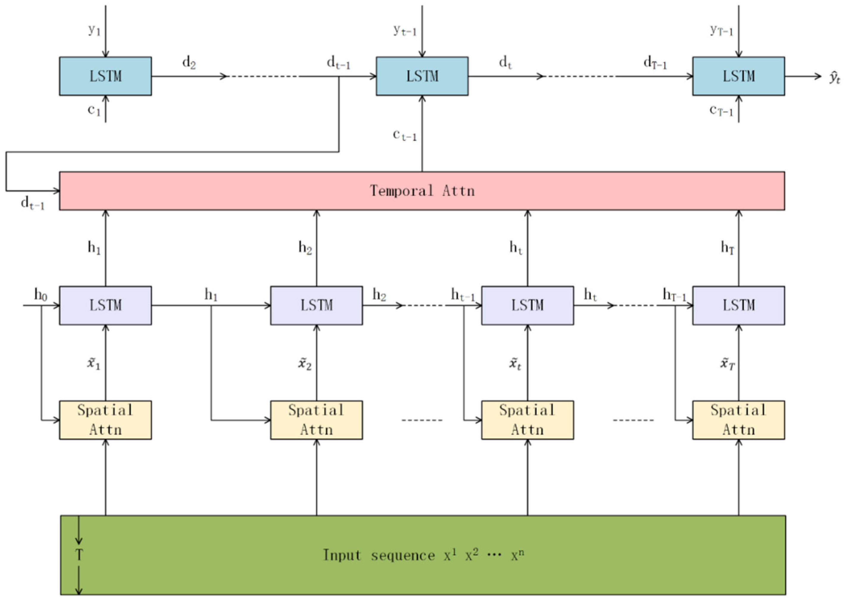
Figure 1 presents the framework of our model. Following the encoder-decoder architecture [11], we built a prediction network based on DA-RNN [16]. The encoder processes a multidimensional spatial attention mechanism that can adaptively capture the dynamic correlation between the Chl-a and other features time series. The decoder uses a temporal attention to adaptively select the relevant previous time intervals for making prediction. With the spatial-temporal attention mechanisms, the DA-RNN can catch the degree of the relevancy between input features and Chl-a and apply the attention of time dimension to catch dynamic temporal correlation.
2.2.1. Encoder with Multidimensional Spatial Attentions
The encoder is essentially an RNN that encodes the input sequences into a feature representation in machine translation [19]. An RNN is a neural network consisting of a hidden state h and an optional output which operates on a variable-length sequence , where n is the number of other features. At each time step t, the hidden state of the RNN is updated by
where is a non-linear activation function, can be an element-wise logistic sigmoid function and also can be a long short-term memory (LSTM) unit [10]. In this paper, we use an LSTM unit as to catch long-term dependencies.
One important property of human perception is that one does not tend to process a whole scene in its entirety at once [20]. Instead humans selectively focus attention on different parts of the visual space to acquire information at the required time and place. Inspired by human beings focusing on the selected parts of attention to obtain the information what they need, we propose a multidimensional spatial attention-based encoder that can adaptively select the relevant features time series. Given the k-th input feature time series , we employ the multidimensional spatial attention mechanism to adaptively capture the correlation between the Chl-a time series and other features input sequences with:
where [.;.] is a concentration operation, and are parameters to learn, is the previous hidden state and is the memory cell state in the encoder LSTM unit. The spatial attention weight can be calculated by Equations (5) and (6) [16]. is the attention weight measuring the importance of the k-th input feature at time step t. Once we obtain the attention weights, we can update the input feature sequences and the hidden state at time t as the following:
where is still an LSTM unit, and is the newly input feature sequences. With this spatial attention mechanism, the encoder can selectively capture the dynamic correlation between the Chl-a and other features rather than treating all the input features equally.
2.2.2. Decoder with Temporal Attentions
In LSTM, only the last hidden state is used for prediction. However, the performance of encoder-decoder architecture will degrade rapidly with the encoder length increases. To solve this issue, a temporal attention mechanism is used in the decoder stage to model the dynamic temporal correlation between different time intervals in the input feature sequence. The attention weight of each encoder hidden state at each time t is defined as follows:
where , and are parameters to learn, is the previous decoder hidden state and is the memory cell state in the decoder LSTM unit. is calculated by Equation (10), it is the importance weight of the i-th encoder hidden state at time t for the prediction [16]. is a weighted sum of all the encoder hidden states. These scores are normalized by a SoftMax function to create the attention mask on the encoder hidden states.
Once the weighted summed context vector at time step t is obtained, we can combine them with the Chl-a time series and update the decoder hidden state.
where and are the parameters to map the concatenation to the size the decoder input, is the decoder input, is the computed context vector, [.;.] is a concentration operation. is the decoder hidden state at time t.
We concatenate the context vector with the hidden state , which becomes the new hidden state from which we make final predictions as follows:
where the matrix and the vector map the concatenation . Finally, we use a linear transformation () to generate the final prediction result. Our approach is smooth and differentiable, and we use the Adam optimizer [21] to train the model by minimizing the mean squared error.
3. Experiment and Results
3.1. Datasets
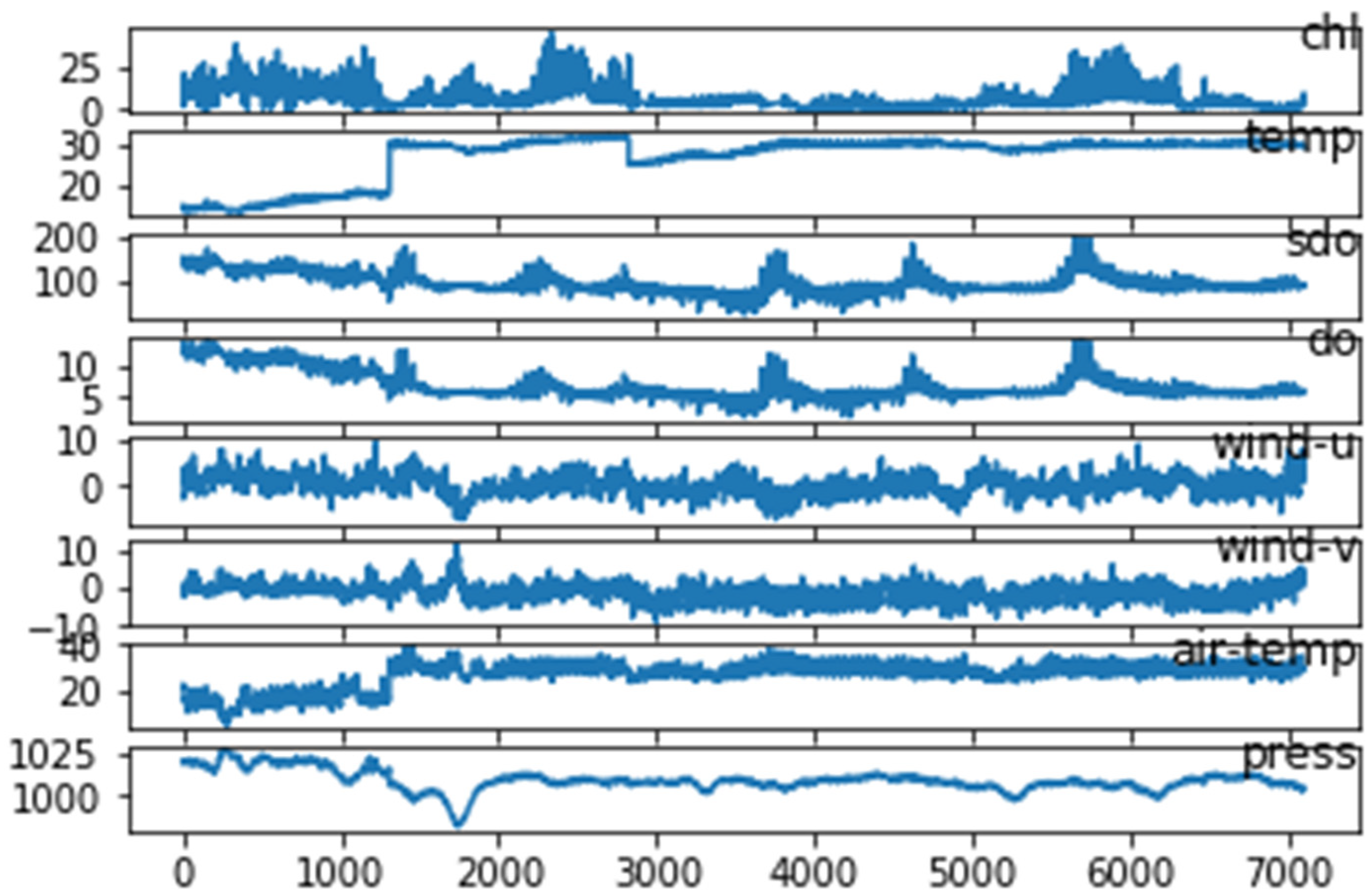
Data used in experiments comes from Fujian Marine Forecasts Station, we use the data from January 2009 to August 2011 as shown in Table 1. In this dataset, the station dimensions have up to 14 different types of sensing data, including SDO (Saturated Dissolved Oxygen), DO (Dissolved Oxygen), Temperature, Salt, Chlorophyll-a (Chl-a), Tides, Turbidity, PH, Air Temperature, Press, WIND_SPEED, WIND_DIRECTION, FLOW_SPEED, and FLOW_DIRECTION. We choose the index of Chlorophyll-a(Chl-a) index as an indicator of the algal biomass, which means we use the Chl-a value as the target series. In order to select the correlation factors related to red tide, we use the Pearson Correlation Coefficient (PCC) to measure the correlation between the related factors and red tide. We choose the higher value of PCC as the related factors, including Air Temperature, SDO, DO, Temperature, Press, Wind Speed, and Wind Direction. Table 2 shows the PCC value between related factors and Chl-a values. Data sensing interval is 30 minutes. The trend of related factors is showed in Figure 2. In the experiments, we partition the data into training and test data by a 9:1 ratio, we use the 6337 data points as the training data, and the 834 data points as the test data. Owing to the discontinuity of the data recorded at the station, also in order to enhance the generalization ability of the model, we decided to shuffle the train data to train our model.
The PCC function is defined as follows:
3.2. Evaluation Metrics and Determination of Parameters
We use two different evaluation metrics to measure the effectiveness of various models for Chl-a time series prediction, including the root mean squared error (RMSE) and the mean absolute error (MAE). The smaller RMSE or MAE of the model, the better its performance. The RMSE function and the MAE function are defined as follows:
In our experiments, we have three hyperparameters, including the length of window size T, the number of hidden states in encoder as m, and the number of hidden states in decoder as p. During the training phase, we set 128 as the size of the minibatch. Firstly, we chose a proper value for the number of hidden states in encoder m and in decoder p from {32,64,128,256}. We discovered that the best performance occurred when m = p = 64 from Table 3. As for the size of window size, we set .
3.3. Experiment-I
We compare our model with the following three baselines:
- BP: Back-propagation neural network (BP) [9] is the most widely used ML method to predict harmful algal blooms. A lot of studies have shown the efficiency of it.
- Seq2seq: It uses an RNN to encode the input sequences into a feature representation and another RNN to make predictions iteratively [19].
- Attention RNN: Attention RNN is the attention-based encoder decoder network that employs an attention mechanism to select parts of hidden states across all the time steps [12].
In this section, we first evaluate the predictive performance of DA-RNN for Chl-a. To be fair, we presented the best performance of each method under different parameter settings in Table 4. We also set different time intervals for comparison, which are 6, 12, 18, and 24. The time series prediction results of DA-RNN and baseline methods over the dataset are shown in Table 4, we can clearly observe that DA-RNN achieves the best performance both on RMSE and MAE when time intervals are 6 and 12 and 18. When the prediction interval is 6, BP performs worst both on RMSE and MAE. When prediction intervals are 12 and 18, Seq2seq always performs the worst both on RMSE and MAE. However, DA-RNN does not always perform the best, when prediction interval is 24, the MAE of DA-RNN is slightly higher (0.848 vs 0.831) than BP, but the RMSE of DA-RNN still performs best, indicating that DA-RNN has more advantages in the long-term predictions than Seq2seq and Attention LSTM and BP.
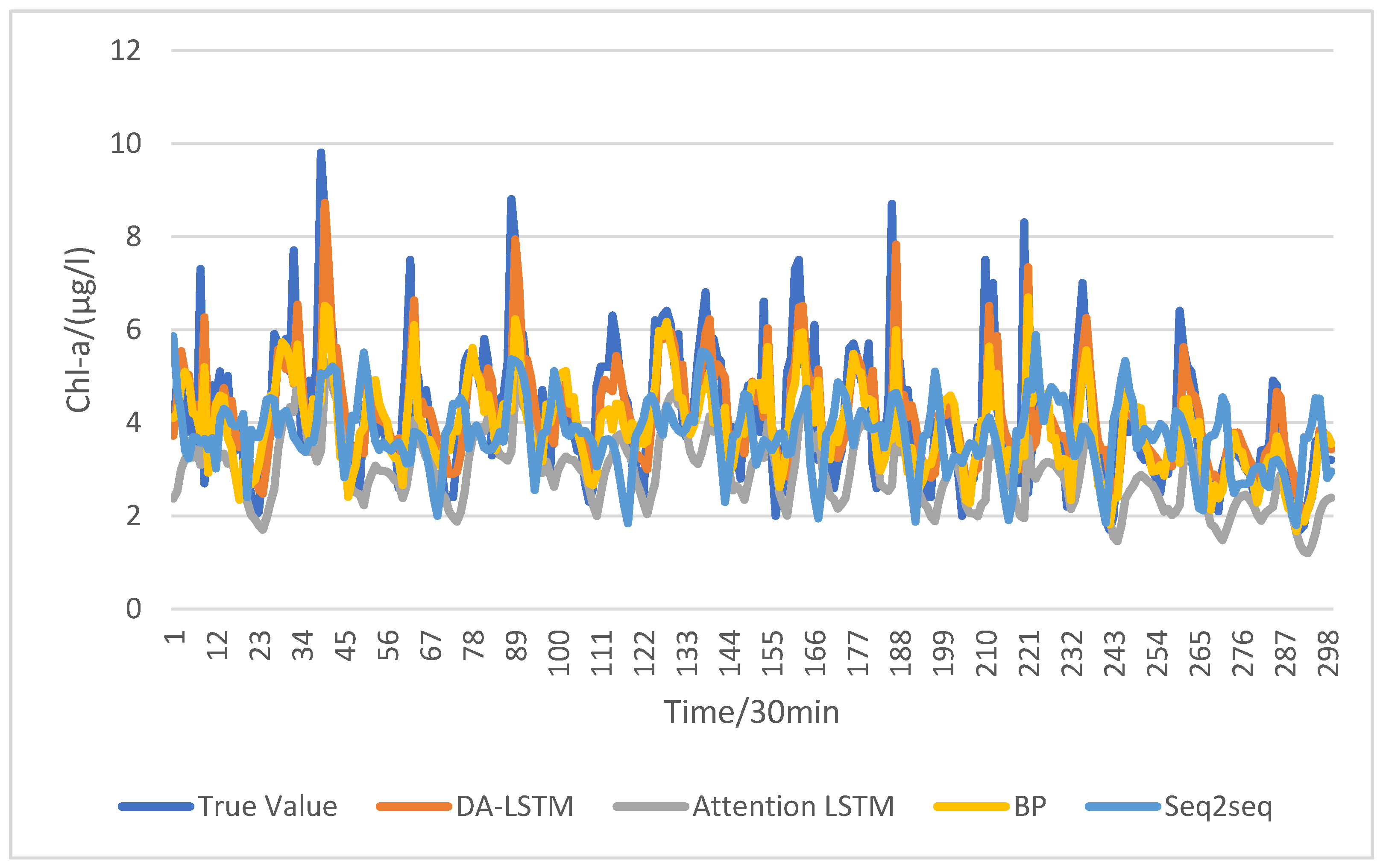
Figure 3 shows the comparison of Chl-a prediction results using four different methods when the time interval is 12. In order to see the comparison results more clearly, we only show the 300 prediction results. The X axis represents the time interval and the Y axis represents the Chl-a value. The dark blue line represents the true value. The orange line represents the prediction results of DA-RNN network. Gray line represents the prediction results of Attention LSTM. The yellow line represents the prediction results of BP network, and the light blue line represents the prediction results of Seq2seq network. As shown in Figure 3, the prediction results of DA-RNN are closer to real values than the other three methods. It also indicates that the DA-RNN can be a good choice for dealing with the Chl-a prediction problem.
3.4. Experiment-II
In Experiment-I, we use Pearson Correlation Coefficient (PCC) to measure the correlation between the related factors and Chl-a. Considering that different factors have different correlation with the Chl-a value, we suspect that different factors may have different correlation with the model errors. We compute the PCC between the model errors and the other factors, as is shown in Table 5.
Comparison to Table 2 and Table 5, we discovered that there is a similarity between the correlation of related factors to Chl-a and related factors to model errors, so we chose the errors between the actual Chl-a value and the prediction Chl-a value using DA-RNN in Experiment-I as the target series. The other 7 different types of sensing data, including of SDO, DO, Temperature, Air Temperature, Press, WIND_SPEED, and WIND_DIRECTION still is chosen as the relevant features. Dataset is still divided into training set and test set according to the ratio of 9:1. Considering the purpose of the error forecast experiment is to predict the forecast reliability of the model and have a basic understanding of the range and fluctuation of model errors, we chose to use the absolute value of the errors to predict in this experiment.
Since the error forecast experiment is based on the experiment-I, we also chose to use the DA-RNN model to forecast the model errors. We still used the same hyperparameters as Experiment-I, which are minibatch = 128, m = p = 32, and we set the time intervals 12 to show our results.
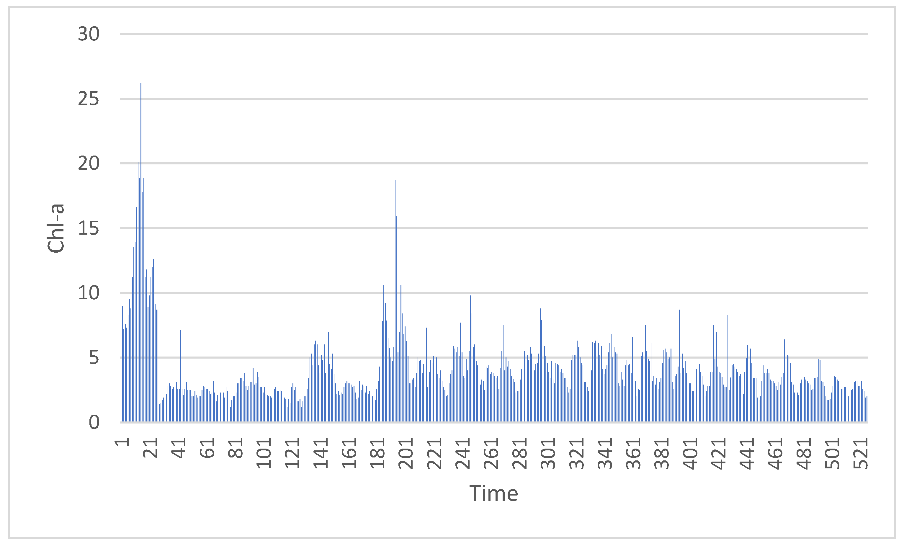
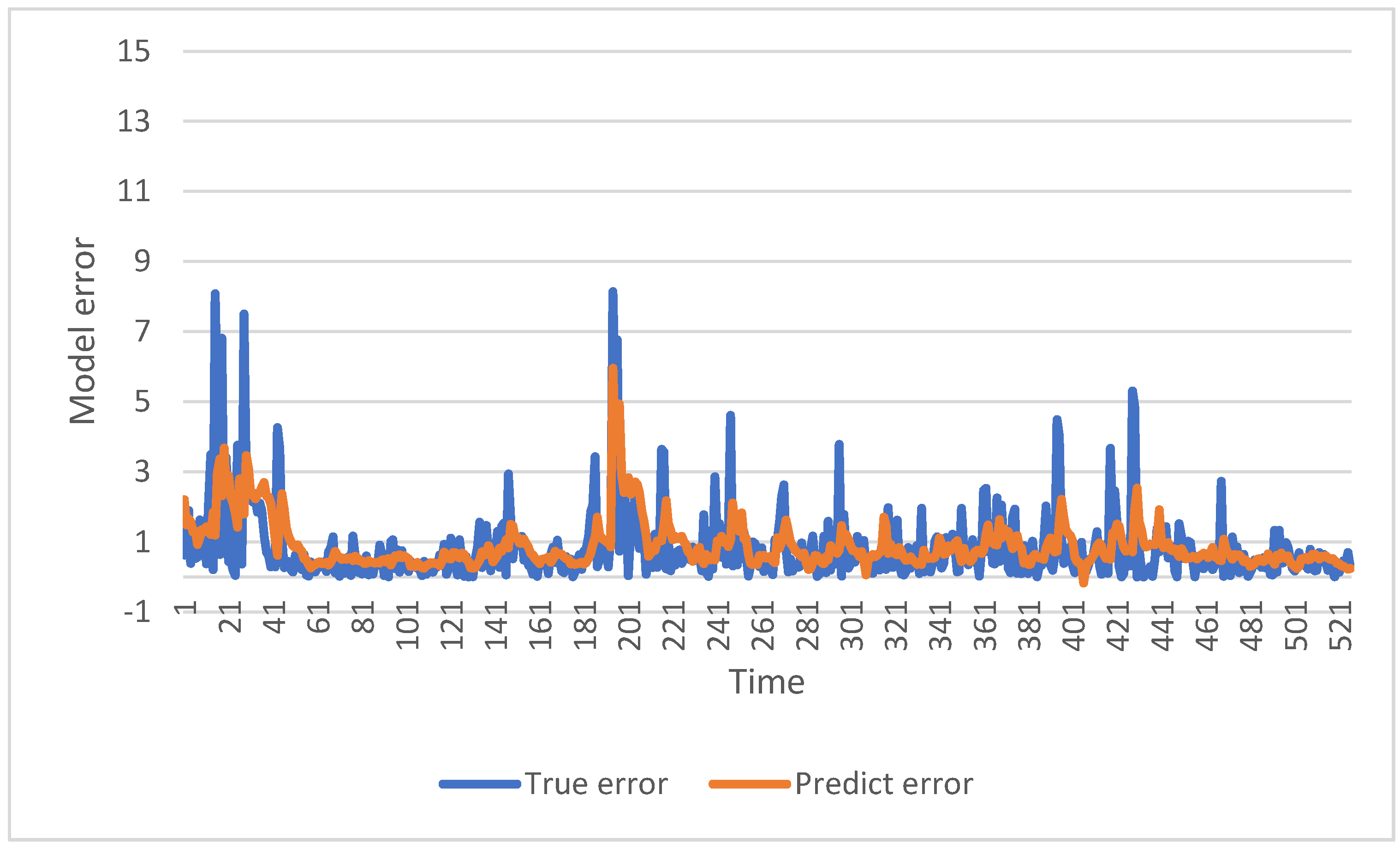
Figure 4 shows the comparison of the predicted errors of 12 intervals with actual errors. The blue line represents the absolute value of actual errors, which are between the real Chl-a value and the prediction Chl-a value using DA-RNN. The orange line represents the prediction errors which are forecasted by DA-RNN. Compared to Figure 4 and Figure 5, we can clearly observe that the fluctuation of Chl-a value is consistent with the fluctuation of experimental error. Figure 5 shows that our method can fit the fluctuation of the model error.
4. Discussion
4.1. The Discussion of Experiment-I
Table 4 reveals that DA-RNN performs better than other methods in most of case, except for the time interval is 24. The reason is that DA-RNN apply the dual-stage attention mechanism. Even with an increase of time interval, the performance of DA-RNN still remain stable instead of degrading rapidly. This shows the superiority of DA-RNN in long time series prediction. The Chl-a value will suddenly rise when the red tide erupts, so it is the most important to know the rising stage of Chl-a value in advance for the red tide prediction. Figure 3 clearly shows that when the time ranges are from 37 to 46, from 82 to 91 and from 181 to 190, which are the time periods that the Chl-a rises suddenly, DA-RNN is always closer to the true value than the other methods, which means when the red tide breaks out, the DA-RNN can always forecast it in advance of other methods. This has great significance to the prevention and control of red tides.
4.1.1. The Influence of Temporal Attention
Based on the experimental results, Attention LSTM always performs better than Seq2seq. The reason is that compared with Seq2seq, Attention LSTM develops a temporal attention mechanism to select parts of hidden states across all the time steps, which can solve the problem that the performance of Seq2seq will deteriorate rapidly as the length of input sequence increases. As is shown in Table 3, when prediction intervals are small, the performance gap between Seq2seq and Attention LSTM is not obvious, however, when prediction intervals increase, the difference of them is significantly increased. The performance of Attention LSTM is almost stable with the time intervals increase. The reason is that the temporal attention mechanism can capture the dynamic influence and solve the long-term dependence problem. The comparison of the prediction results of Seq2seq and Attention LSTM show the superiority and necessity of temporal attention mechanism.
4.1.2. The Influence of Multidimensional Spatial Attention
It is kindly obvious that RMSE and MAE of DA-RNN are significantly better than those of Attention LSTM. Figure 3 also shows that the prediction results using the DA-RNN are closer to the real Chl-a observations than the Attention LSTM model.
The reason is that Attention LSTM treats all the input factors equally, different factors have different influence weights on the prediction of Chl-a value is not considered. Considering that Chl-a is related to many other dimensions of meteorological factors, such as pressure, light, wind speed, wind direct, and air temperature, a multidimensional spatial attention mechanism to adaptively capture the dynamic correlation between such factors and Chl-a is necessary. To address this issue, the multidimensional spatial attention mechanism module is developed to select the relevant factors input sequences. Figure 3 also reveals that DA-RNN can capture the sudden change of Chl-a much better in advance than other methods. It indicates that multidimensional spatial attention mechanism is always beneficial to forecast the red tides.
4.1.3. Comparison with BP Network
BP network is the most widely used machine learning method to predict harmful algal blooms. BP can handle well the nonlinear relationship between water quality indicators and Chl-a concentration, of which many studies have shown the efficiency. The Table 4 and Figure 3 show that DA-RNN has higher prediction accuracy and lower RMSE and MAE than BP network. This illustrates DA-RNN can be a good choice for dealing with Chl-a prediction problem.
4.2. The Discussion of Experiment-II
Because the cost and loss caused by red tide disaster are huge, the instability of red tide prediction needs to be forecasted in advance, so DA-RNN is applied to predict the fluctuation of model errors, which can provide a reference for the forecast reliability.
Figure 4 shows the changes of Chl-a value a period of times, when time ranges are from 1 to 35 and from 188 to 205, the Chl-a value fluctuates greatly. Figure 5 clearly shows that from 1 to 35 and from 188 to 205, even the prediction errors of the DA-RNN model also fluctuate greatly. It indicates that the fluctuation of Chl-a value is consistent with the fluctuation of experimental errors. The blue line in Figure 5 represents the actual model errors, the orange line represents the model errors that we forecast. We can clearly observe that the orange line could fit the trend of the blue line. When time ranges are from 1 to 35 and from 188 to 205, the errors of the model fluctuate greatly. The orange line can fit the huge fluctuation of model errors at these time period, which provides a basis for the reliability of our model prediction scheme.
In the future, we may extract the large part of the prediction errors and retrain them to achieve a better fitting result through the result of the error forecast.
5. Conclusions
In this paper, we proposed a spatial-temporal attention mechanism model for Chlorophyll-a(Chl-a) concentration prediction. Seven water parameters related to algal bloom problems are considered, dataset used in experiments comes from Fujian Marine Forecasts Station. Using the HABs data, the model can both adaptively select the relevant input factors sequences and select the relevant previous time intervals for making prediction. We used Fujian Marine Forecasts Station’s 2009–2011 dataset to evaluate the model, and the result proves that our model performs better than the other methods (Seq2seq and Attention LSTM and BP) both on RMSE and MAE in most cases. When the red tide breaks out, DA-RNN can capture the sudden change of Chl-a much better in advance than other methods. The results showed that our prediction models can well handle the nonlinear relationship between water quality indicators and Chl-a concentration. DA-RNN is also applied to forecast the prediction errors of the model and aims to predict the forecast reliability of the model, as well as to have a basic understanding of the range and fluctuation of model errors, which can provide a reference to describe the range of meteorological disasters.
Author Contributions
The authors contributed equally to the preparation of the manuscript and the concept of the research. The writing of the draft was by X.W. and L.X.; the review and editing of the draft were done by X.W. All authors have read and agreed to the published version of the manuscript.
Funding
This research was funded by National Program on Key Research Project, grant number 2016YFC1401900.
Acknowledgments
Thanks for the hard work of editor and reviewers’ comments to improve the paper.
Conflicts of Interest
The authors declare no conflict of interest.
References
- Amin, R.; Penta, B.; de Rada, S. Occurrence and Spatial Extent of HABs on the West Florida Shelf 2002–Present. IEEE Geosci. Remote Sens. Lett. 2015, 12, 2080–2084. [Google Scholar] [CrossRef]
- Gao, W.; Yao, Z. Prediction of algae growth based on BP neural networks. Computer 2005, 21, 167–169. [Google Scholar]
- Qin, R.; Lin, L. Integration of GIS and a Lagrangian Particle-Tracking Model for Harmful Algal Bloom Trajectories Prediction. Water 2019, 11, 164. [Google Scholar] [CrossRef] [Green Version]
- Gokaraju, B.; Durbha, S.S.; King, R.L.; Younan, N.H. A machine learning based spatio-temporal data mining approach for detection of harmful algal blooms in the Gulf of Mexico. IEEE J. Sel. Top. Appl. Earth Obs. Remote Sens. 2011, 4, 710–720. [Google Scholar] [CrossRef]
- Park, S.; Kwon, J.; Jeong, J.G.; Lee, S.R. Red tides prediction using fuzzy inference and decision tree. In Proceedings of the 2012 International Conference on ICT Convergence (ICTC), Jeju Island, Korea, 15–17 October 2012; pp. 493–498. [Google Scholar]
- Yang, M.; Ishizaka, J.; Goes, J.; Gomes, H.; Maúre, E.; Hayashi, M.; Katano, T.; Fujii, N.; Saitoh, K.; Mine, T. Improved MODIS-Aqua chlorophyll-a retrievals in the turbid semi-enclosed Ariake Bay, Japan. Remote Sens. 2018, 10, 1335. [Google Scholar] [CrossRef] [Green Version]
- Lee, J.H.; Huang, Y.; Dickman, M.; Jayawardena, A. Neural network modelling of coastal algal blooms. Ecol. Model. 2003, 159, 179–201. [Google Scholar] [CrossRef]
- Wei, B.; Sugiura, N.; Maekawa, T. Use of artificial neural network in the prediction of algal blooms. Water Res. 2001, 35, 2022–2028. [Google Scholar] [CrossRef]
- Werbos, P. Beyond Regression: New Tools for Prediction and Analysis in the Behavioral Sciences. Ph.D. Thesis, Harvard University, Cambridge, MA, USA, 1974. [Google Scholar]
- Hochreiter, S.; Schmidhuber, J. Long short-term memory. Neural Comput. 1997, 9, 1735–1780. [Google Scholar] [CrossRef] [PubMed]
- Cho, K.; Van Merriënboer, B.; Gulcehre, C.; Bahdanau, D.; Bougares, F.; Schwenk, H.; Bengio, Y. Learning phrase representations using RNN encoder-decoder for statistical machine translation. arXiv 2014, arXiv:1406.1078. [Google Scholar]
- Bahdanau, D.; Cho, K.; Bengio, Y. Neural machine translation by jointly learning to align and translate. arXiv 2014, arXiv:1409.0473. [Google Scholar]
- Li, W.; Liu, P.; Zhang, Q.; Liu, W. An Improved Approach for Text Sentiment Classification Based on a Deep Neural Network via a Sentiment Attention Mechanism. Future Internet 2019, 11, 96. [Google Scholar] [CrossRef] [Green Version]
- Zhang, Q.; Lu, R. A Multi-Attention Network for Aspect-Level Sentiment Analysis. Future Internet 2019, 11, 157. [Google Scholar] [CrossRef] [Green Version]
- Xu, H.; Ding, Y.; Sun, J.; Zhao, K.; Chen, Y. Dynamic Group Recommendation Based on the Attention Mechanism. Future Internet 2019, 11, 198. [Google Scholar] [CrossRef] [Green Version]
- Qin, Y.; Song, D.; Chen, H.; Cheng, W.; Jiang, G.; Cottrell, G. A dual-stage attention-based recurrent neural network for time series prediction. arXiv 2017, arXiv:1704.02971. [Google Scholar]
- Liang, Y.; Ke, S.; Zhang, J.; Yi, X.; Zheng, Y. GeoMAN: Multi-level Attention Networks for Geo-sensory Time Series Prediction. In Proceedings of the Twenty-Seventh International Joint Conference on Artificial Intelligence (IJCAI-18), Stockholm, Sweden, 13–19 July 2018; pp. 3428–3434. [Google Scholar]
- Liu, J.; Zhang, T.; Han, G.; Gou, Y. TD-LSTM: Temporal Dependence-Based LSTM Networks for Marine Temperature Prediction. Sensors 2018, 18, 3797. [Google Scholar] [CrossRef] [Green Version]
- Sutskever, I.; Vinyals, O.; Le, Q. Sequence to Sequence Learning with Neural Networks. In Proceedings of the Advances in Neural Information Processing Systems, Montreal, QC, Canada, 8–13 December 2014. [Google Scholar]
- Mnih, V.; Heess, N.; Graves, A. Recurrent Models of Visual Attention. In Proceedings of the Advances in Neural Information Processing Systems, Montreal, QC, Canada, 8–13 December 2014; pp. 2204–2212. [Google Scholar]
- Kingma, D.P.; Ba, J. Adam: A method for stochastic optimization. arXiv 2014, arXiv:1412.6980. [Google Scholar]
Figure 1.
DA-RNN networks architecture.

Figure 2.
The trend of related factors.

Figure 3.
Chl-a prediction using different methods (12 time intervals).

Figure 4.
The Chl-a value and its fluctuations.

Figure 5.
Comparison of the predicted errors with actual errors.


Table 1.
Details of the dataset.
| Dataset | Fujian Marine Forecasts Station | |
| Attributes | 8 | |
| Target Series | Chlorophyll-a | |
| Time Intervals | 30 min | |
| Time Spans | 18/01/2009–27/08/2011 | |
| Size | train | 6337 |
| test | 834 | |
Table 2.
PCC between Chl-a and related factors.
| SDO | DO | Temperature | Air-Temperature | Press | Wind-Speed | Wind-Direction | |
|---|---|---|---|---|---|---|---|
| PCC | 0.381 | 0.438 | −0.372 | −0.365 | 0.253 | 0.177 | 0.210 |
Table 3.
Parameter determination.
| m = p | Prediction Intervals | ||||
|---|---|---|---|---|---|
| 6 | 12 | 18 | 24 | ||
| 32 | RMSE | 1.265 | 1.229 | 1.233 | 1.29 |
| MAE | 0.795 | 0.819 | 0.836 | 0.855 | |
| 64 | RMSE | 1.269 | 1.201 | 1.205 | 1.215 |
| MAE | 0.79 | 0.778 | 0.814 | 0.848 | |
| 128 | RMSE | 1.286 | 1.255 | 1.321 | 1.322 |
| MAE | 0.819 | 0.909 | 0.939 | 0.904 | |
| 256 | RMSE | 1.389 | 1.285 | 1.345 | 1.404 |
| MAE | 0.834 | 1.017 | 1.104 | 1.112 | |
Table 4.
Prediction results of different time intervals.
| Models | Metrics | Prediction Intervals | |||
|---|---|---|---|---|---|
| 6 | 12 | 18 | 24 | ||
| Seq2seq | RMSE | 1.398 | 1.411 | 1.456 | 1.499 |
| MAE | 0.922 | 0.972 | 0.993 | 1.027 | |
| Attention LSTM | RMSE | 1.29 | 1.254 | 1.305 | 1.32 |
| MAE | 0.837 | 0.855 | 0.894 | 0.902 | |
| BP | RMSE | 1.404 | 1.207 | 1.256 | 1.28 |
| MAE | 1.12 | 0.854 | 0.816 | 0.831 | |
| DA-RNN | RMSE | 1.269 | 1.201 | 1.205 | 1.215 |
| MAE | 0.79 | 0.778 | 0.814 | 0.848 | |
Table 5.
PCC between model error and related factors.
| SDO | DO | Temperature | Air-Temperature | Press | Wind-Speed | Wind-Direction | |
|---|---|---|---|---|---|---|---|
| PCC | 0.252 | 0.241 | −0.137 | −0.124 | 0.092 | 0.121 | 0.10 |
© 2020 by the authors. Licensee MDPI, Basel, Switzerland. This article is an open access article distributed under the terms and conditions of the Creative Commons Attribution (CC BY) license (http://creativecommons.org/licenses/by/4.0/).
Share and Cite
MDPI and ACS Style
Wang, X.; Xu, L. Unsteady Multi-Element Time Series Analysis and Prediction Based on Spatial-Temporal Attention and Error Forecast Fusion. Future Internet 2020, 12, 34. https://0-doi-org.brum.beds.ac.uk/10.3390/fi12020034
AMA Style
Wang X, Xu L. Unsteady Multi-Element Time Series Analysis and Prediction Based on Spatial-Temporal Attention and Error Forecast Fusion. Future Internet. 2020; 12(2):34. https://0-doi-org.brum.beds.ac.uk/10.3390/fi12020034
Chicago/Turabian StyleWang, Xiaofan, and Lingyu Xu. 2020. "Unsteady Multi-Element Time Series Analysis and Prediction Based on Spatial-Temporal Attention and Error Forecast Fusion" Future Internet 12, no. 2: 34. https://0-doi-org.brum.beds.ac.uk/10.3390/fi12020034
Note that from the first issue of 2016, this journal uses article numbers instead of page numbers. See further details here.