An Updated Survey of Efficient Hardware Architectures for Accelerating Deep Convolutional Neural Networks

 , , , , and
Abstract
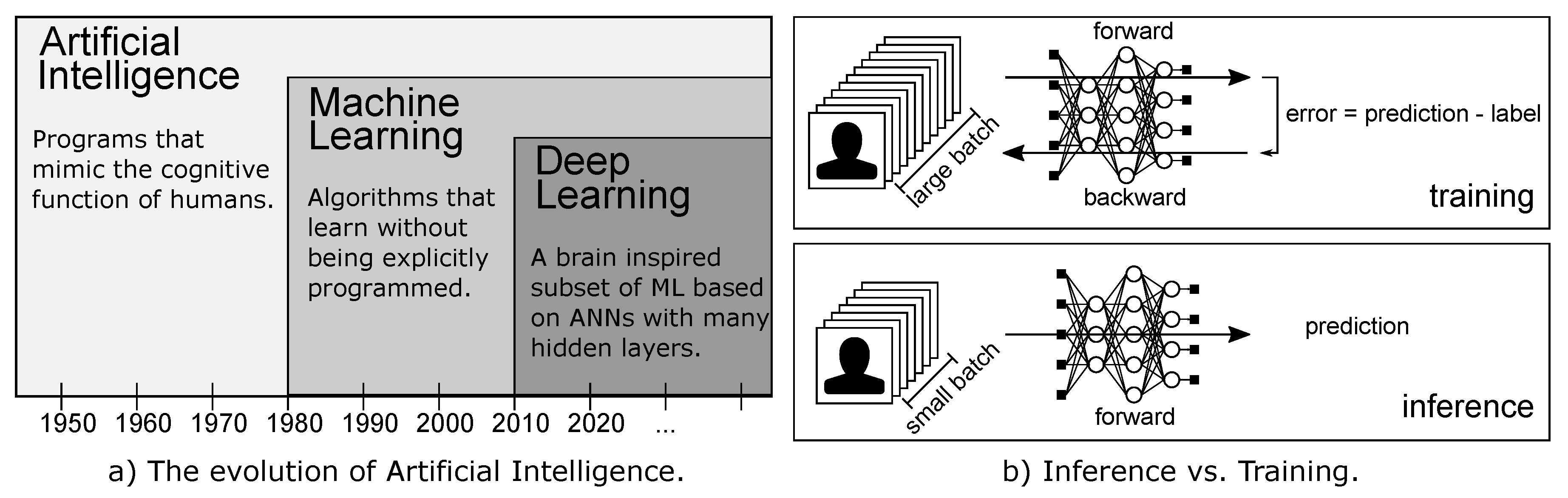
:1. Introduction
2. Background: Deep Neural Networks
2.1. Training and Inference
- Forward pass: the input is fed into the network that produces an output.
- Backward pass: a loss L is computed comparing the produced output and the desired output. The loss L is then used for the backpropagation algorithm [28], that applying the chain rule of calculus computes the gradient for each weight (and bias) of the network.
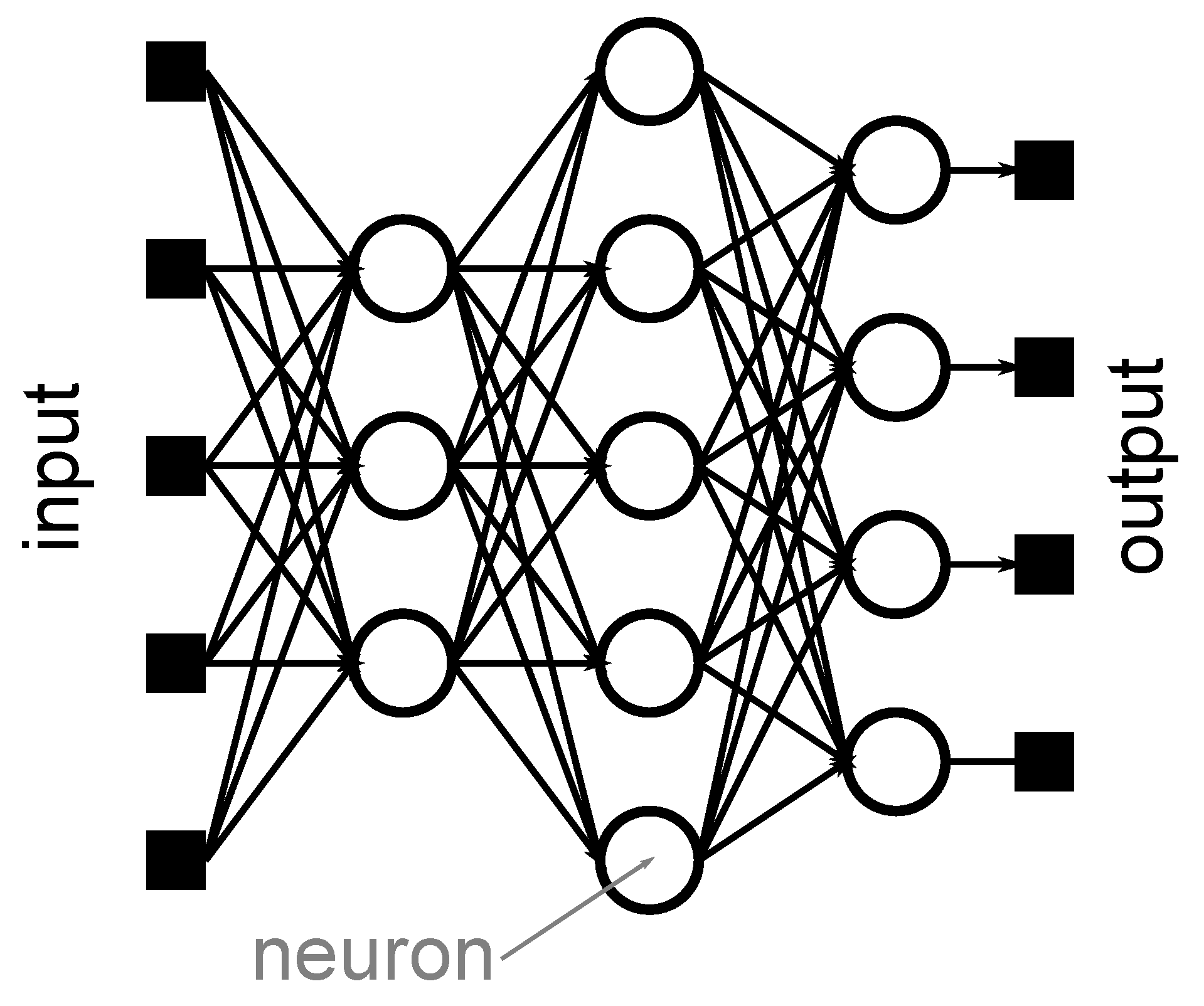
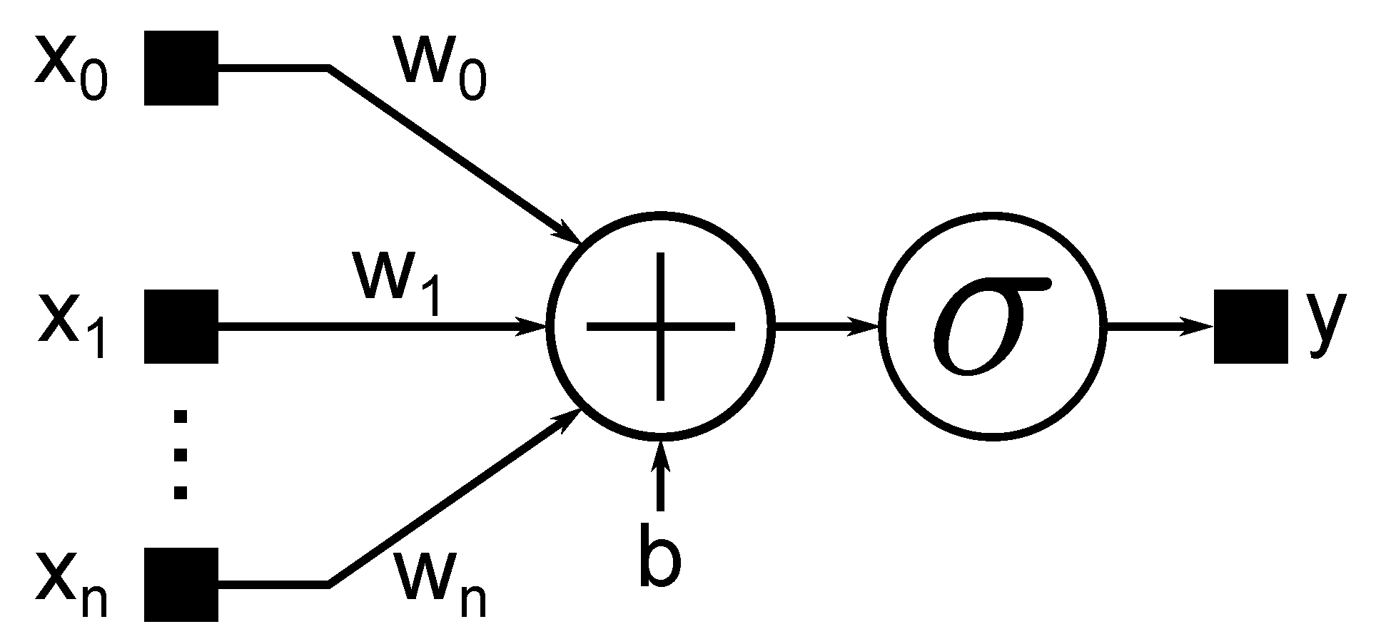
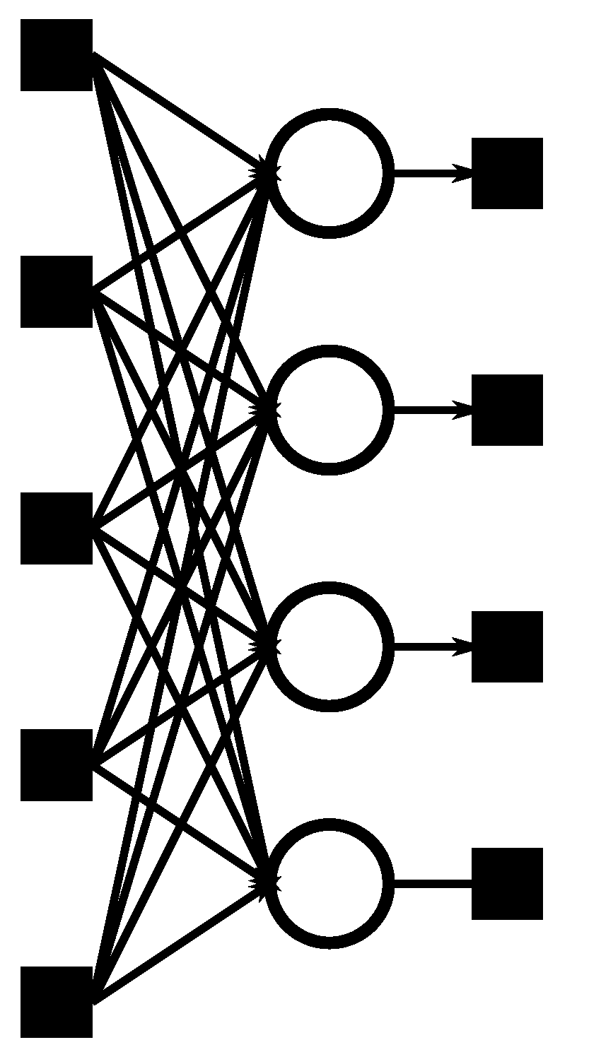
2.2. Layers
2.3. DNN Models
3. Energy-Efficient Architectures
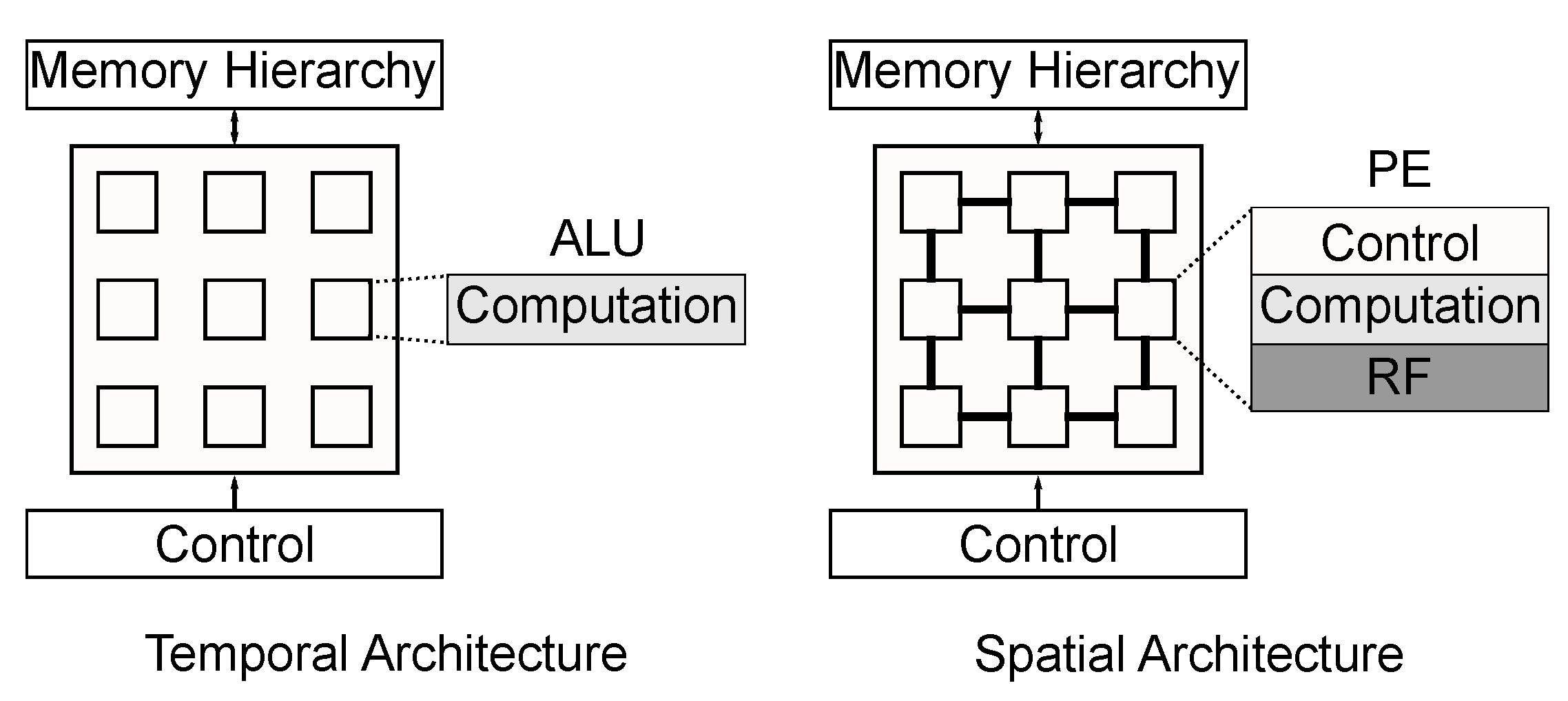
3.1. Temporal Architectures
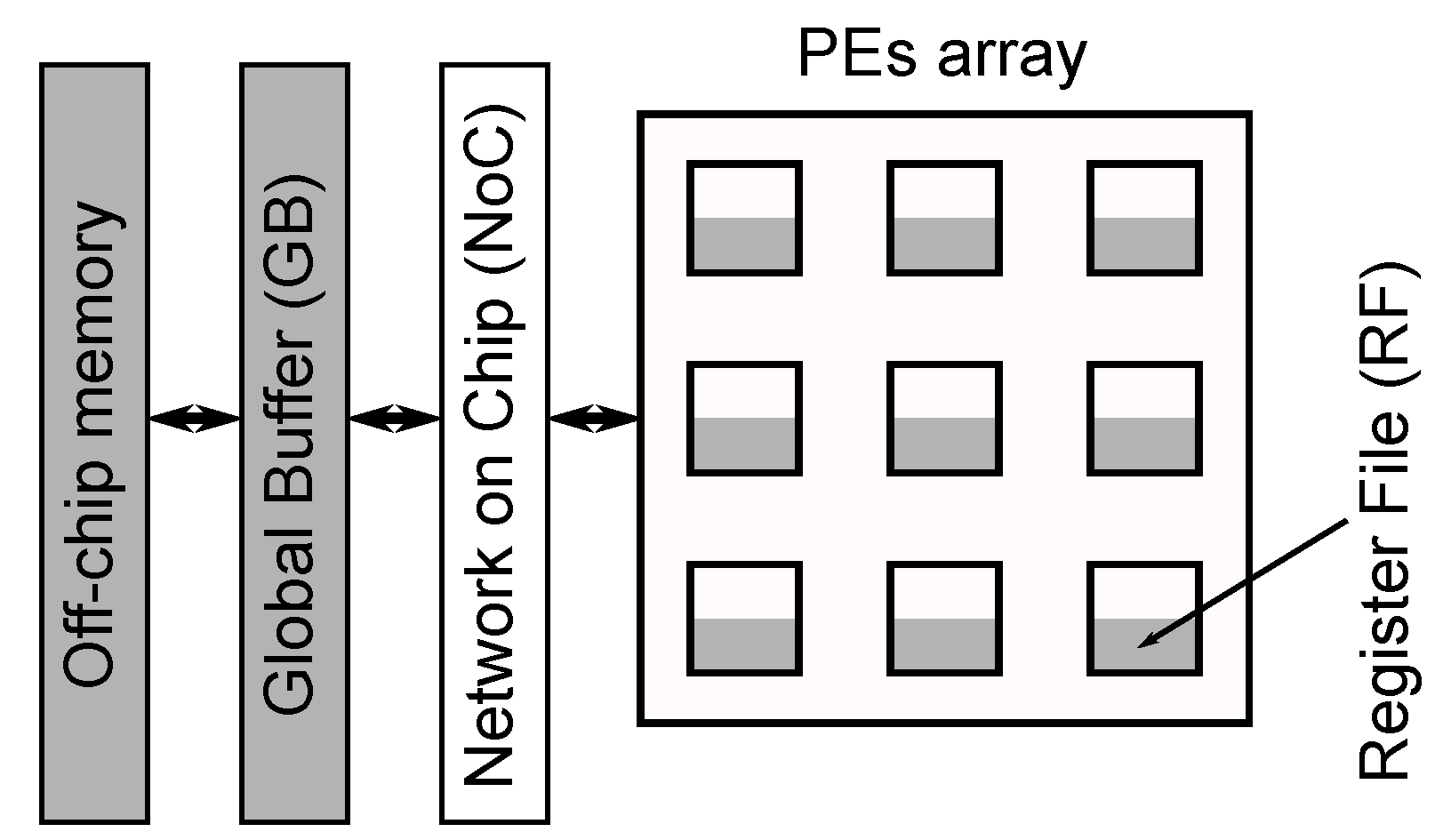
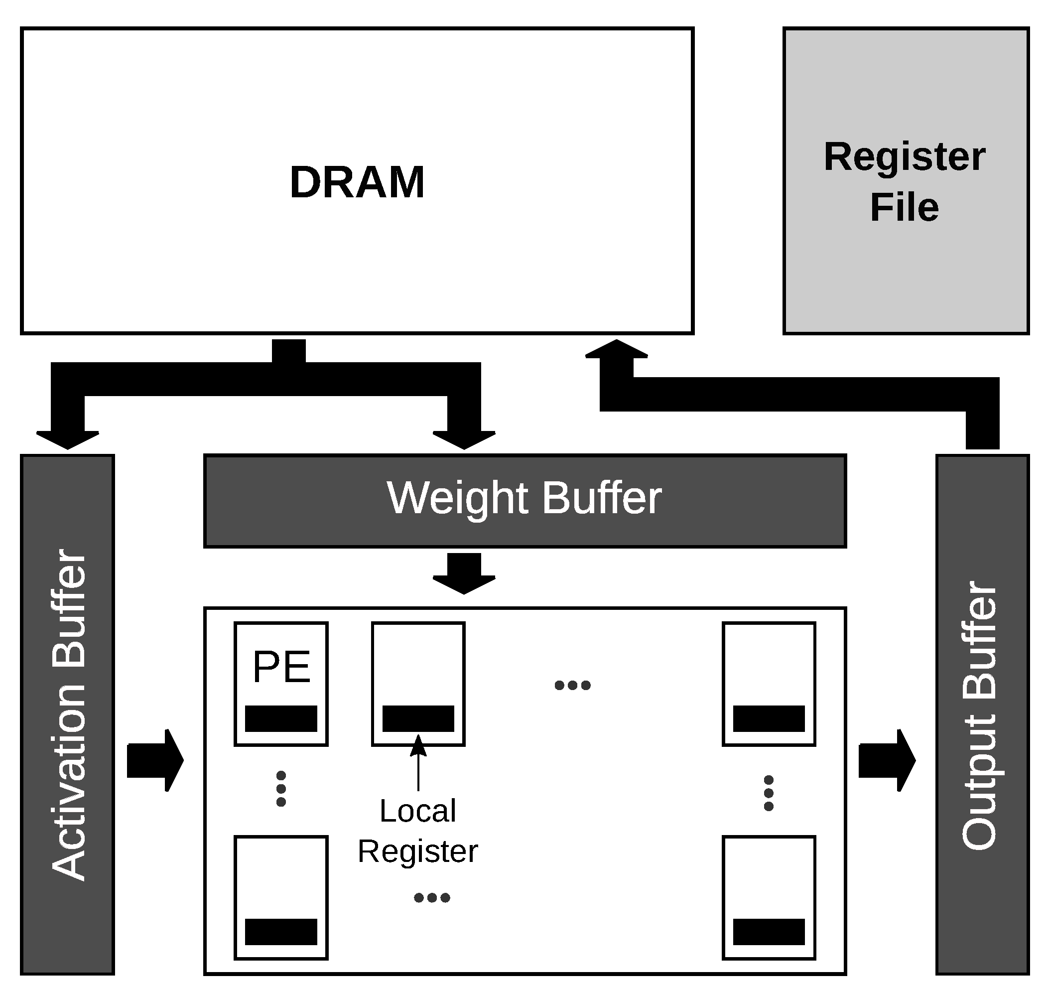
3.2. Spatial Architectures: Fpgas and Asics
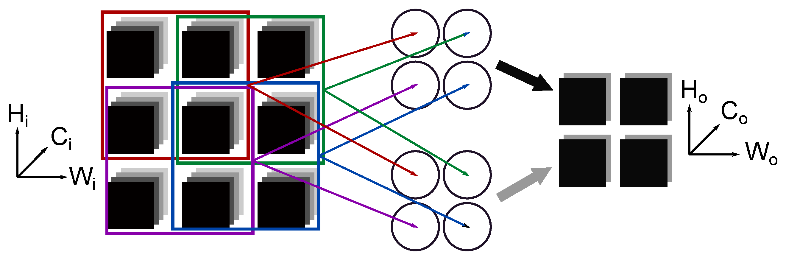
- Weight reuse: a kernel of weights is reused HoxWo times for each sub-grid of the input feature maps;
- Input reuse: the input feature maps are reused Co times to compute each output feature map.
- Convolutional reuse: when the weight kernel slides through the input feature maps, the sub-grids used for computation usually overlap. The input values that fall in the overlapping region are reused to compute two or more output values.
- Weight Stationary (WS): the weights are stored in the RFs of the PEs and kept fixed, while the inputs are distributed coordinated with the movement of the partial sums between the PEs to obtain the correct results. These accelerators exploit weight reuse and convolutional reuse. Popular WS accelerators are [59,60].
- Row Stationary (RS): this dataflow jointly maximizes the reuse of all data, i.e., inputs, weights, and partial sums. In this dataflow, the operations of a row of the convolution are mapped to the same PE. The weights are kept stationary in the PEs. For instance, Eyeriss [63] is an RS accelerator.
- No Local Reuse (NLR): This dataflow reduces the accelerator area by eliminating the RFs from the PEs and reading data only from GBs. There is no data reuse. DianNao [64] is an NLR accelerator.
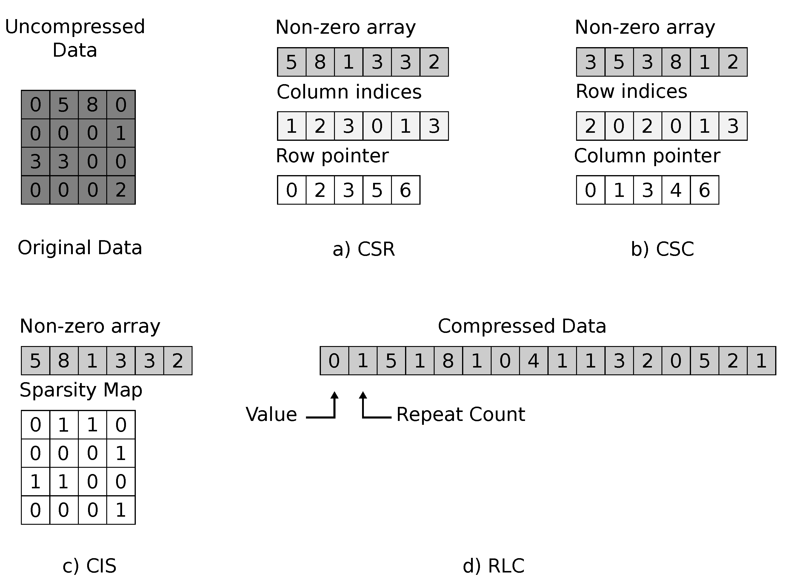
3.2.1. Accelerators with Sparsity Exploitation
3.2.2. Variable Bitwidth Accelerators
3.2.3. Reconfigurable Accelerators
4. Memory
5. Hardware Metrics and Comparison
6. Conclusions
Author Contributions
Funding
Acknowledgments
Conflicts of Interest
Appendix A

| AI | Artificial Intelligence | GPU | Graphic Processing Unit |
| ALU | Arithmetic Logic Unit | IFM | Input Feature Map |
| ANN | Artificial Neural Network | IoT | Internet of Things |
| ASIC | Application Specific Integrated Circuit | LIM | Logic in Memory |
| BLAS | Basic Linear Algebra Subroutines | MAC | Multiply-and-Accumulate |
| BN | Batch Normalization | ML | Machine Learning |
| CIS | Compressed Image Size | MMAC | Matrix Multiply-and-Accumulate |
| CNN | Convolution Neural Networks | NLP | Natural Language Processing |
| Conv | Convolutional | NLR | No Local Reuse |
| CPU | Central Processing Unit | NN | Neural Network |
| CSC | Compressed Sparse Column | OFM | Output Feature Map |
| CSR | Compressed Sparse Row | OS | Output Stationary |
| DL | Deep Learning | PE | Processing Element |
| DNN | Deep Neural Network | ReLU | Rectified Linear Unit |
| DRAM | Dynamic Random Access Memory | RF | Register File |
| FC | Fully Connected | RLC | Run Length Coding |
| FFT | Fast Fourier Transform | RS | Row Stationary |
| FM | Feature Map | SIMD | Single-Instruction Multiple-Data |
| FPGA | Field Programmable Gate Array | SIMT | Single-Instruction Multiple-Threads |
| GB | Global Buffer | VLSI | Very Large Scale Integration |
| GeMM | General Matrix Multiplication | WS | Weight Stationary |
References
- LeCun, Y.; Bengio, Y.; Hinton, G. Deep Learning. Nature 2015, 521, 436–444. [Google Scholar] [CrossRef] [PubMed]
- Zanc, R.; Cioara, T.; Anghel, I. Forecasting Financial Markets using Deep Learning. In Proceedings of the 2019 IEEE 15th International Conference on Intelligent Computer Communication and Processing (ICCP), Cluj-Napoca, Romania, 5–7 September 2019; pp. 459–466. [Google Scholar]
- Ying, J.J.; Huang, P.; Chang, C.; Yang, D. A preliminary study on deep learning for predicting social insurance payment behavior. In Proceedings of the 2017 IEEE International Conference on Big Data (Big Data), Boston, MA, USA, 11–14 December 2017; pp. 1866–1875. [Google Scholar]
- Ha, V.; Lu, D.; Choi, G.S.; Nguyen, H.; Yoon, B. Improving Credit Risk Prediction in Online Peer-to-Peer (P2P) Lending Using Feature selection with Deep learning. In Proceedings of the 2019 21st International Conference on Advanced Communication Technology (ICACT), PyeongChang Kwangwoon_Do, Korea, 17–20 February 2019; pp. 511–515. [Google Scholar]
- Arslan, A.K.; Yaşar, Ş.; Çolak, C. An Intelligent System for the Classification of Lung Cancer Based on Deep Learning Strategy. In Proceedings of the 2019 International Artificial Intelligence and Data Processing Symposium (IDAP), Malatya, Turkey, 21–22 September 2019; pp. 1–4. [Google Scholar]
- Mohsen, H.; El-Dahshan, E.S.; El-Horbarty, E.S.M.; Salem, A.B. Classification using Deep Learning Neural Networks for Brain Tumors. Future Comput. Inform. J. 2018, 3, 68–71. [Google Scholar] [CrossRef]
- Barata, C.; Marques, J.S. Deep Learning For Skin Cancer Diagnosis With Hierarchical Architectures. In Proceedings of the 2019 IEEE 16th International Symposium on Biomedical Imaging (ISBI 2019), Venice, Italy, 8–11 April 2019; pp. 841–845. [Google Scholar]
- Grigorescu, S.; Trasnea, B.; Cocias, T.; Macesanu, G. A survey of deep learning techniques for autonomous driving. J. Field Robot. 2020, 37, 362–386. [Google Scholar] [CrossRef]
- Palossi, D.; Loquercio, A.; Conti, F.; Flamand, E.; Scaramuzza, D.; Benini, L. Ultra Low Power Deep-Learning-powered Autonomous Nano Drones. arXiv 2018, arXiv:1805.01831. [Google Scholar]
- Zhang, D.; Liu, S. Top-Down Saliency Object Localization Based on Deep-Learned Features. In Proceedings of the 2018 11th International Congress on Image and Signal Processing, BioMedical Engineering and Informatics (CISP-BMEI), Beijing, China, 13–15 October 2018; pp. 1–9. [Google Scholar]
- Minaee, S.; Boykov, Y.; Porikli, F.; Plaza, A.; Kehtarnavaz, N.; Terzopoulos, D. Image Segmentation Using Deep Learning: A Survey. arXiv 2020, arXiv:2001.05566. [Google Scholar]
- Kaskavalci, H.C.; Gören, S. A Deep Learning Based Distributed Smart Surveillance Architecture using Edge and Cloud Computing. In Proceedings of the 2019 International Conference on Deep Learning and Machine Learning in Emerging Applications (Deep-ML), Istanbul, Turkey, 26–28 August 2019; pp. 1–6. [Google Scholar]
- Capra, M.; Peloso, R.; Masera, G.; Ruo Roch, M.; Martina, M. Edge Computing: A Survey On the Hardware Requirements in the Internet of Things World. Future Internet 2019, 11, 100. [Google Scholar] [CrossRef] [Green Version]
- Shafique, M.; Theocharides, T.; Bouganis, C.; Hanif, M.A.; Khalid, F.; Hafız, R.; Rehman, S. An overview of next-generation architectures for machine learning: Roadmap, opportunities and challenges in the IoT era. In Proceedings of the 2018 Design, Automation Test in Europe Conference Exhibition (DATE), Dresden, Germany, 19–23 March 2018; pp. 827–832. [Google Scholar]
- Marchisio, A.; Hanif, M.A.; Khalid, F.; Plastiras, G.; Kyrkou, C.; Theocharides, T.; Shafique, M. Deep Learning for Edge Computing: Current Trends, Cross-Layer Optimizations, and Open Research Challenges. In Proceedings of the 2019 IEEE Computer Society Annual Symposium on VLSI (ISVLSI), Miami, FL, USA, 15–17 July 2019; pp. 553–559. [Google Scholar]
- Zhang, J.J.; Liu, K.; Khalid, F.; Hanif, M.A.; Rehman, S.; Theocharides, T.; Artussi, A.; Shafique, M.; Garg, S. Building Robust Machine Learning Systems: Current Progress, Research Challenges, and Opportunities. In Proceedings of the 56th Annual Design Automation Conference, Las Vegas, NV, USA, 2–6 June 2019. [Google Scholar]
- Shafique, M.; Naseer, M.; Theocharides, T.; Kyrkou, C.; Mutlu, O.; Orosa, L.; Choi, J. Robust Machine Learning Systems: Challenges, Current Trends, Perspectives, and the Road Ahead. IEEE Des. Test 2020, 37, 30–57. [Google Scholar] [CrossRef]
- Sze, V.; Chen, Y.; Yang, T.; Emer, J.S. Efficient Processing of Deep Neural Networks: A Tutorial and Survey. Proc. IEEE 2017, 105, 2295–2329. [Google Scholar] [CrossRef] [Green Version]
- Deng, B.L.; Li, G.; Han, S.; Shi, L.; Xie, Y. Model Compression and Hardware Acceleration for Neural Networks: A Comprehensive Survey. Proc. IEEE 2020, 108, 485–532. [Google Scholar] [CrossRef]
- Schuman, C.D.; Potok, T.E.; Patton, R.M.; Birdwell, J.D.; Dean, M.E.; Rose, G.S.; Plank, J.S. A Survey of Neuromorphic Computing and Neural Networks in Hardware. arXiv 2017, arXiv:1705.06963. [Google Scholar]
- Chen, Y.; Xie, Y.; Song, L.; Chen, F.; Tang, T. A Survey of Accelerator Architectures for Deep Neural Networks. Engineering 2020, 6, 264–274. [Google Scholar] [CrossRef]
- Han, S.; Mao, H.; Dally, W.J. Deep Compression: Compressing Deep Neural Network with Pruning, Trained Quantization and Huffman Coding. arXiv 2015, arXiv:1510.00149. [Google Scholar]
- Cai, H.; Gan, C.; Han, S. Once for All: Train One Network and Specialize it for Efficient Deployment. arXiv 2019, arXiv:1908.09791. [Google Scholar]
- Parashar, A.; Rhu, M.; Mukkara, A.; Puglielli, A.; Venkatesan, R.; Khailany, B.; Emer, J.; Keckler, S.W.; Dally, W.J. SCNN: An accelerator for compressed-sparse convolutional neural networks. In Proceedings of the 2017 ACM/IEEE 44th Annual International Symposium on Computer Architecture (ISCA), Toronto, ON, Canada, 24–28 June 2017; pp. 27–40. [Google Scholar] [CrossRef]
- Li, J.; Jiang, S.; Gong, S.; Wu, J.; Yan, J.; Yan, G.; Li, X. SqueezeFlow: A Sparse CNN Accelerator Exploiting Concise Convolution Rules. IEEE Trans. Comput. 2019, 68, 1663–1677. [Google Scholar] [CrossRef]
- Aimar, A.; Mostafa, H.; Calabrese, E.; Rios-Navarro, A.; Tapiador-Morales, R.; Lungu, I.; Milde, M.B.; Corradi, F.; Linares-Barranco, A.; Liu, S.; et al. NullHop: A Flexible Convolutional Neural Network Accelerator Based on Sparse Representations of Feature Maps. IEEE Trans. Neural Netw. Learn. Syst. 2019, 30, 644–656. [Google Scholar] [CrossRef] [Green Version]
- Bengio, Y. Learning Deep Architectures for AI. Found. Trends Mach. Learn. 2009, 2, 1–127. [Google Scholar] [CrossRef]
- Lecun, Y.; Bottou, L.; Bengio, Y.; Haffner, P. Gradient-Based Learning Applied to Document Recognition. Proc. IEEE 1998, 86, 2278–2324. [Google Scholar] [CrossRef] [Green Version]
- Qian, N. On the momentum term in gradient descent learning algorithms. Neural Netw. 1999, 12, 145–151. [Google Scholar] [CrossRef]
- Kingma, D.; Ba, J. Adam: A Method for Stochastic Optimization. In Proceedings of the International Conference on Learning Representations, Banff, AB, Canada, 14–16 April 2014. [Google Scholar]
- Krizhevsky, A.; Sutskever, I.; Hinton, G.E. ImageNet Classification with Deep Convolutional Neural Networks. In Proceedings of the 25th International Conference on Neural Information Processing Systems—Volume 1; Curran Associates Inc.: Red Hook, NY, USA, 2012; pp. 1097–1105. [Google Scholar]
- Russakovsky, O.; Deng, J.; Su, H.; Krause, J.; Satheesh, S.; Ma, S.; Huang, Z.; Karpathy, A.; Khosla, A.; Bernstein, M.; et al. ImageNet Large Scale Visual Recognition Challenge. Int. J. Comput. Vis. 2015, 115, 211–252. [Google Scholar] [CrossRef] [Green Version]
- Simonyan, K.; Zisserman, A. Very Deep Convolutional Networks for Large-Scale Image Recognition. arXiv 2014, arXiv:1409.1556. [Google Scholar]
- Szegedy, C.; Liu, W.; Jia, Y.; Sermanet, P.; Reed, S.; Anguelov, D.; Erhan, D.; Vanhoucke, V.; Rabinovich, A. Going deeper with convolutions. In Proceedings of the 2015 IEEE Conference on Computer Vision and Pattern Recognition (CVPR), Boston, MA, USA, 7–12 June 2015; pp. 1–9. [Google Scholar]
- Szegedy, C.; Vanhoucke, V.; Ioffe, S.; Shlens, J.; Wojna, Z. Rethinking the Inception Architecture for Computer Vision. In 2016 IEEE Conference on Computer Vision and Pattern Recognition, CVPR 2016, Las Vegas, NV, USA, 27–30 June 2016; IEEE Computer Society: Washington, DC, USA, 2016; pp. 2818–2826. [Google Scholar] [CrossRef] [Green Version]
- Szegedy, C.; Ioffe, S.; Vanhoucke, V.; Alemi, A.A. Inception-v4, Inception-ResNet and the Impact of Residual Connections on Learning. In Proceedings of the Thirty-First AAAI Conference on Artificial Intelligence, San Francisco, CA, USA, 4–9 February 2017; Singh, S.P., Markovitch, S., Eds.; AAAI Press: Palo Alto, CA, USA, 2017; pp. 4278–4284. [Google Scholar]
- He, K.; Zhang, X.; Ren, S.; Sun, J. Deep Residual Learning for Image Recognition. In Proceedings of the 2016 IEEE Conference on Computer Vision and Pattern Recognition (CVPR), Las Vegas, NV, USA, 27–30 June 2016; pp. 770–778. [Google Scholar]
- Chollet, F. Xception: Deep Learning with Depthwise Separable Convolutions. In Proceedings of the 2017 IEEE Conference on Computer Vision and Pattern Recognition (CVPR), Honolulu, HI, USA, 21–26 July 2017; pp. 1800–1807. [Google Scholar]
- Xie, S.; Girshick, R.; Dollár, P.; Tu, Z.; He, K. Aggregated Residual Transformations for Deep Neural Networks. In Proceedings of the 2017 IEEE Conference on Computer Vision and Pattern Recognition (CVPR), Honolulu, HI, USA, 21–26 July 2017; pp. 5987–5995. [Google Scholar] [CrossRef] [Green Version]
- Huang, G.; Liu, Z.; Weinberger, K.Q. Densely Connected Convolutional Networks. In Proceedings of the 2017 IEEE Conference on Computer Vision and Pattern Recognition (CVPR), Honolulu, HI, USA, 21–26 July 2017; pp. 2261–2269. [Google Scholar]
- Hu, J.; Shen, L.; Sun, G. Squeeze-and-Excitation Networks. In Proceedings of the 2018 IEEE/CVF Conference on Computer Vision and Pattern Recognition, Salt Lake City, UT, USA, 18–22 June 2018; pp. 7132–7141. [Google Scholar] [CrossRef] [Green Version]
- Zoph, B.; Vasudevan, V.; Shlens, J.; Le, Q.V. Learning Transferable Architectures for Scalable Image Recognition. In Proceedings of the 2018 IEEE Conference on Computer Vision and Pattern Recognition, CVPR 2018, Salt Lake City, UT, USA, 18–22 June 2018; IEEE Computer Society: Washington, DC, USA, 2018; pp. 8697–8710. [Google Scholar] [CrossRef] [Green Version]
- Devlin, J.; Chang, M.; Lee, K.; Toutanova, K. BERT: Pre-training of Deep Bidirectional Transformers for Language Understanding. In 2019 Conference of the North American Chapter of the Association for Computational Linguistics: Human Language Technologies, NAACL-HLT 2019, Minneapolis, MN, USA, 2–7 June 2019, Volume 1 (Long and Short Papers); Burstein, J., Doran, C., Solorio, T., Eds.; Association for Computational Linguistics: Stroudsburg, PA, USA, 2019; pp. 4171–4186. [Google Scholar]
- Shoeybi, M.; Patwary, M.; Puri, R.; LeGresley, P.; Casper, J.; Catanzaro, B. Megatron-LM: Training Multi-Billion Parameter Language Models Using Model Parallelism. arXiv 2019, arXiv:1909.08053. [Google Scholar]
- Rodriguez, A.; Segal, E.; Meiri, E.; Fomenko, E.; Kim, Y.; Shen, H.; Ziv, B. Lower Numerical Precision Deep Learning Inference and Training. Intel White Paper 2018, 3, 1–19. [Google Scholar]
- Chellapilla, K.; Puri, S.; Simard, P. High Performance Convolutional Neural Networks for Document Processing. In Tenth International Workshop on Frontiers in Handwriting Recognition; Lorette, G., Ed.; Université de Rennes 1, Suvisoft: La Baule, France, 2006; Available online: http://www.suvisoft.com (accessed on 7 June 2020).
- Vasudevan, A.; Anderson, A.; Gregg, D. Parallel Multi Channel convolution using General Matrix Multiplication. In Proceedings of the 2017 IEEE 28th International Conference on Application-specific Systems, Architectures and Processors (ASAP), Seattle, WA, USA, 10–12 July 2017; pp. 19–24. [Google Scholar]
- Mathieu, M.; Henaff, M.; LeCun, Y. Fast Training of Convolutional Networks through FFTs. arXiv 2013, arXiv:1312.5851. [Google Scholar]
- James, R. Intel AVX-512 Instructions. 2017. Available online: https://software.intel.com/content/www/cn/zh/develop/articles/intel-avx-512-instructions.html (accessed on 6 June 2020).
- bfloat16—Hardware Numerics Definition. 2018. Available online: https://software.intel.com/content/www/us/en/develop/download/bfloat16-hardware-numerics-definition.html (accessed on 6 June 2020).
- Gogar, S.L. BigDL—Scale-out Deep Learning on Apache Spark* Cluster. 2017. Available online: https://software.intel.com/content/www/us/en/develop/articles/bigdl-scale-out-deep-learning-on-apache-spark-cluster.html (accessed on 6 June 2020).
- Jia, Y.; Shelhamer, E.; Donahue, J.; Karayev, S.; Long, J.; Girshick, R.B.; Guadarrama, S.; Darrell, T. Caffe: Convolutional Architecture for Fast Feature Embedding. In Proceedings of the ACM International Conference on Multimedia, MM’14, Orlando, FL, USA, 3–7 November 2014; Hua, K.A., Rui, Y., Steinmetz, R., Hanjalic, A., Natsev, A., Zhu, W., Eds.; ACM: New York, NY, USA, 2014; pp. 675–678. [Google Scholar] [CrossRef]
- Abadi, M.; Agarwal, A.; Barham, P.; Brevdo, E.; Chen, Z.; Citro, C.; Corrado, G.S.; Davis, A.; Dean, J.; Devin, M.; et al. TensorFlow: Large-Scale Machine Learning on Heterogeneous Systems. 2015. Available online: tensorflow.org (accessed on 6 June 2020).
- Paszke, A.; Gross, S.; Chintala, S.; Chanan, G.; Yang, E.; DeVito, Z.; Lin, Z.; Desmaison, A.; Antiga, L.; Lerer, A. Automatic Differentiation in PyTorch. In Proceedings of the NIPS 2017 Workshop on Autodiff, Long Beach, CA, USA, 4–9 December 2017. [Google Scholar]
- Chetlur, S.; Woolley, C.; Vandermersch, P.; Cohen, J.; Tran, J.; Catanzaro, B.; Shelhamer, E. cuDNN: Efficient Primitives for Deep Learning. arXiv 2014, arXiv:1410.0759. [Google Scholar]
- Available online: https://developer.nvidia.com/gpu-accelerated-libraries (accessed on 6 June 2020).
- NVIDIA TESLA V100 GPU ARCHITECTURE. 2017. Available online: https://images.nvidia.com/content/technologies/volta/pdf/437317-Volta-V100-DS-NV-US-WEB.pdf (accessed on 6 June 2020).
- NVIDIA A100 Tensor Core GPU Architecture. 2020. Available online: https://www.nvidia.com/content/dam/en-zz/Solutions/Data-Center/nvidia-ampere-architecture-whitepaper.pdf (accessed on 6 June 2020).
- Gokhale, V.; Jin, J.; Dundar, A.; Martini, B.; Culurciello, E. A 240 G-ops/s Mobile Coprocessor for Deep Neural Networks. In Proceedings of the 2014 IEEE Conference on Computer Vision and Pattern Recognition Workshops, Columbus, OH, USA, 23–28 June 2014; pp. 696–701. [Google Scholar] [CrossRef]
- Jouppi, N.P.; Young, C.; Patil, N.; Patterson, D.; Agrawal, G.; Bajwa, R.; Bates, S.; Bhatia, S.; Boden, N.; Borchers, A.; et al. In-Datacenter Performance Analysis of a Tensor Processing Unit. SIGARCH Comput. Archit. News 2017, 45, 1–12. [Google Scholar] [CrossRef] [Green Version]
- Du, Z.; Fasthuber, R.; Chen, T.; Ienne, P.; Li, L.; Luo, T.; Feng, X.; Chen, Y.; Temam, O. ShiDianNao: Shifting vision processing closer to the sensor. In Proceedings of the 2015 ACM/IEEE 42nd Annual International Symposium on Computer Architecture (ISCA), Portland, OR, USA, 13–17 June 2015; pp. 92–104. [Google Scholar] [CrossRef]
- Cavigelli, L.; Benini, L. Origami: A 803-GOp/s/W Convolutional Network Accelerator. IEEE Trans. Circuits Syst. Video Technol. 2017, 27, 2461–2475. [Google Scholar] [CrossRef] [Green Version]
- Chen, Y.; Krishna, T.; Emer, J.S.; Sze, V. Eyeriss: An Energy-Efficient Reconfigurable Accelerator for Deep Convolutional Neural Networks. IEEE J. Solid-State Circuits 2017, 52, 127–138. [Google Scholar] [CrossRef] [Green Version]
- Chen, T.; Du, Z.; Sun, N.; Wang, J.; Wu, C.; Chen, Y.; Temam, O. DianNao: A Small-Footprint High-Throughput Accelerator for Ubiquitous Machine-Learning. Int. Conf. Archit. Support Program. Lang. Oper. Syst. 2014, 49, 269–284. [Google Scholar] [CrossRef]
- Han, S.; Pool, J.; Tran, J.; Dally, W.J. Learning Both Weights and Connections for Efficient Neural Networks. In Proceedings of the 28th International Conference on Neural Information Processing Systems—Volume 1; MIT Press: Cambridge, MA, USA, 2015; pp. 1135–1143. [Google Scholar]
- Srinivas, S.; Babu, R.V. Data-free Parameter Pruning for Deep Neural Networks. In Proceedings of the British Machine Vision Conference 2015, BMVC 2015, Swansea, UK, 7–10 September 2015; Xie, X., Jones, M.W., Tam, G.K.L., Eds.; BMVA Press: South Road, Durham, 2015; pp. 31.1–31.12. [Google Scholar] [CrossRef] [Green Version]
- Marchisio, A.; Hanif, M.A.; Martina, M.; Shafique, M. PruNet: Class-Blind Pruning Method For Deep Neural Networks. In Proceedings of the 2018 International Joint Conference on Neural Networks (IJCNN), Rio de Janeiro, Brazil, 8–13 July 2018; pp. 1–8. [Google Scholar]
- Albericio, J.; Judd, P.; Hetherington, T.; Aamodt, T.; Jerger, N.E.; Moshovos, A. Cnvlutin: Ineffectual-Neuron-Free Deep Neural Network Computing. In Proceedings of the 2016 ACM/IEEE 43rd Annual International Symposium on Computer Architecture (ISCA), Seoul, Korea, 18–22 June 2016; pp. 1–13. [Google Scholar] [CrossRef]
- Zhang, S.; Du, Z.; Zhang, L.; Lan, H.; Liu, S.; Li, L.; Guo, Q.; Chen, T.; Chen, Y. Cambricon-X: An accelerator for sparse neural networks. In Proceedings of the 2016 49th Annual IEEE/ACM International Symposium on Microarchitecture (MICRO), Taipei, Taiwan, 15–19 October 2016; pp. 1–12. [Google Scholar] [CrossRef]
- Gondimalla, A.; Chesnut, N.; Thottethodi, M.; Vijaykumar, T.N. SparTen: A Sparse Tensor Accelerator for Convolutional Neural Networks. In Proceedings of the 52nd Annual IEEE/ACM International Symposium on Microarchitecture, Columbus, OH, USA, 12–16 October 2019; Association for Computing Machinery: New York, NY, USA, 2019; pp. 151–165. [Google Scholar] [CrossRef]
- Han, S.; Liu, X.; Mao, H.; Pu, J.; Pedram, A.; Horowitz, M.A.; Dally, W.J. EIE: Efficient Inference Engine on Compressed Deep Neural Network. In Proceedings of the 43rd ACM/IEEE Annual International Symposium on Computer Architecture, ISCA 2016, Seoul, Korea, 18–22 June 2016; IEEE Computer Society: Washington, DC, USA, 2016; pp. 243–254. [Google Scholar] [CrossRef] [Green Version]
- Kim, D.; Ahn, J.; Yoo, S. ZeNA: Zero-Aware Neural Network Accelerator. IEEE Des. Test 2018, 35, 39–46. [Google Scholar] [CrossRef]
- Chen, Y.; Yang, T.; Emer, J.; Sze, V. Eyeriss v2: A Flexible Accelerator for Emerging Deep Neural Networks on Mobile Devices. IEEE J. Emerg. Sel. Top. Circuits Syst. 2019, 9, 292–308. [Google Scholar] [CrossRef] [Green Version]
- Hegde, K.; Yu, J.; Agrawal, R.; Yan, M.; Pellauer, M.; Fletcher, C. UCNN: Exploiting Computational Reuse in Deep Neural Networks via Weight Repetition. In Proceedings of the 2018 ACM/IEEE 45th Annual International Symposium on Computer Architecture (ISCA), Angeles, CA, USA, 1–6 June 2018; pp. 674–687. [Google Scholar]
- Granas, A.; Dugundji, J. Fixed Point Theory; Springer: Berlin/Heidelberg, Germany, 2003. [Google Scholar]
- Horowitz, M. 1.1 Computing’s energy problem (and what we can do about it). In Proceedings of the 2014 IEEE International Solid-State Circuits Conference Digest of Technical Papers (ISSCC), San Francisco, CA, USA, 9–13 February 2014; pp. 10–14. [Google Scholar] [CrossRef]
- Hanif, M.A.; Marchisio, A.; Arif, T.; Hafiz, R.; Rehman, S.; Shafique, M. X-DNNs: Systematic Cross-Layer Approximations for Energy-Efficient Deep Neural Networks. J. Low Power Electron. 2018, 14, 520–534. [Google Scholar] [CrossRef]
- Gysel, P.; Pimentel, J.; Motamedi, M.; Ghiasi, S. Ristretto: A Framework for Empirical Study of Resource-Efficient Inference in Convolutional Neural Networks. IEEE Trans. Neural Netw. Learn. Syst. 2018, 29, 5784–5789. [Google Scholar] [CrossRef] [PubMed]
- Jacob, B.; Kligys, S.; Chen, B.; Zhu, M.; Tang, M.; Howard, A.; Adam, H.; Kalenichenko, D. Quantization and Training of Neural Networks for Efficient Integer-Arithmetic-Only Inference. In Proceedings of the 2018 IEEE/CVF Conference on Computer Vision and Pattern Recognition, Salt Lake City, UT, USA, 18–23 June 2018; pp. 2704–2713. [Google Scholar] [CrossRef] [Green Version]
- Sankaradas, M.; Jakkula, V.; Cadambi, S.; Chakradhar, S.; Durdanovic, I.; Cosatto, E.; Graf, H.P. A Massively Parallel Coprocessor for Convolutional Neural Networks. In Proceedings of the 2009 20th IEEE International Conference on Application-specific Systems, Architectures and Processors, Boston, MA, USA, 7–9 July 2009; pp. 53–60. [Google Scholar] [CrossRef]
- Sakr, C.; Shanbhag, N. Per-Tensor Fixed-Point Quantization of the Back-Propagation Algorithm. arXiv 2019, arXiv:1812.11732. [Google Scholar]
- Judd, P.; Albericio, J.; Moshovos, A. Stripes: Bit-Serial Deep Neural Network Computing. IEEE Comput. Archit. Lett. 2017, 16, 80–83. [Google Scholar] [CrossRef]
- Lee, J.; Kim, C.; Kang, S.; Shin, D.; Kim, S.; Yoo, H. UNPU: An Energy-Efficient Deep Neural Network Accelerator With Fully Variable Weight Bit Precision. IEEE J. Solid-State Circuits 2019, 54, 173–185. [Google Scholar] [CrossRef]
- Sharify, S.; Lascorz, A.D.; Siu, K.; Judd, P.; Moshovos, A. Loom: Exploiting Weight and Activation Precisions to Accelerate Convolutional Neural Networks. In Proceedings of the 2018 55th ACM/ESDA/IEEE Design Automation Conference (DAC), San Francisco, CA, USA, 24–28 June 2018; pp. 1–6. [Google Scholar]
- Sharma, H.; Park, J.; Suda, N.; Lai, L.; Chau, B.; Chandra, V.; Esmaeilzadeh, H. Bit Fusion: Bit-Level Dynamically Composable Architecture for Accelerating Deep Neural Network. In Proceedings of the 2018 ACM/IEEE 45th Annual International Symposium on Computer Architecture (ISCA), Los Angeles, CA, USA, 1–6 June 2018; pp. 764–775. [Google Scholar]
- Ryu, S.; Kim, H.; Yi, W.; Kim, J. BitBlade: Area and Energy-Efficient Precision-Scalable Neural Network Accelerator with Bitwise Summation. In Proceedings of the 2019 56th ACM/IEEE Design Automation Conference (DAC), Las Vegas, NV, USA, 2–6 June 2019; pp. 1–6. [Google Scholar]
- Lu, W.; Yan, G.; Li, J.; Gong, S.; Han, Y.; Li, X. FlexFlow: A Flexible Dataflow Accelerator Architecture for Convolutional Neural Networks. In Proceedings of the 2017 IEEE International Symposium on High Performance Computer Architecture (HPCA), Austin, TX, USA, 4–8 February 2017; pp. 553–564. [Google Scholar]
- Tu, F.; Yin, S.; Ouyang, P.; Tang, S.; Liu, L.; Wei, S. Deep Convolutional Neural Network Architecture With Reconfigurable Computation Patterns. IEEE Trans. Very Large Scale Integr. (VLSI) Syst. 2017, 25, 2220–2233. [Google Scholar] [CrossRef]
- Hanif, M.A.; Putra, R.V.W.; Tanvir, M.; Hafiz, R.; Rehman, S.; Shafique, M. MPNA: A Massively-Parallel Neural Array Accelerator with Dataflow Optimization for Convolutional Neural Networks. arXiv 2018, arXiv:1810.12910. [Google Scholar]
- Yin, S.; Ouyang, P.; Tang, S.; Tu, F.; Li, X.; Liu, L.; Wei, S. A 1.06-to-5.09 TOPS/W reconfigurable hybrid-neural-network processor for deep learning applications. In Proceedings of the 2017 Symposium on VLSI Circuits, Kyoto, Japan, 5–8 June 2017; pp. C26–C27. [Google Scholar]
- Fowers, J.; Ovtcharov, K.; Papamichael, M.; Massengill, T.; Liu, M.; Lo, D.; Alkalay, S.; Haselman, M.; Adams, L.; Ghandi, M.; et al. A Configurable Cloud-Scale DNN Processor for Real-Time AI. In Proceedings of the 2018 ACM/IEEE 45th Annual International Symposium on Computer Architecture (ISCA), Los Angeles, CA, USA, 1–6 June 2018; pp. 1–14. [Google Scholar]
- Kwon, H.; Samajdar, A.; Krishna, T. MAERI: Enabling Flexible Dataflow Mapping over DNN Accelerators via Reconfigurable Interconnects. In Proceedings of the Twenty-Third International Conference on Architectural Support for Programming Languages and Operating Systems; Association for Computing Machinery: New York, NY, USA, 2018; pp. 461–475. [Google Scholar] [CrossRef]
- Qin, E.; Samajdar, A.; Kwon, H.; Nadella, V.; Srinivasan, S.; Das, D.; Kaul, B.; Krishna, T. SIGMA: A Sparse and Irregular GEMM Accelerator with Flexible Interconnects for DNN Training. In Proceedings of the 2020 IEEE International Symposium on High Performance Computer Architecture (HPCA), San Diego, CA, USA, 22–26 February 2020; pp. 58–70. [Google Scholar]
- Shin, D.; Lee, J.; Lee, J.; Lee, J.; Yoo, H. DNPU: An Energy-Efficient Deep-Learning Processor with Heterogeneous Multi-Core Architecture. IEEE Micro 2018, 38, 85–93. [Google Scholar] [CrossRef]
- Stoutchinin, A.; Conti, F.; Benini, L. Optimally Scheduling CNN Convolutions for Efficient Memory Access. arXiv 2019, arXiv:1902.01492. [Google Scholar]
- Li, J.; Yan, G.; Lu, W.; Jiang, S.; Gong, S.; Wu, J.; Li, X. SmartShuttle: Optimizing off-chip memory accesses for deep learning accelerators. In Proceedings of the 2018 Design, Automation Test in Europe Conference Exhibition (DATE), Dresden, Germany, 19–23 March 2018; pp. 343–348. [Google Scholar] [CrossRef]
- Putra, R.V.W.; Hanif, M.A.; Shafique, M. DRMap: A Generic DRAM Data Mapping Policy for Energy-Efficient Processing of Convolutional Neural Networks. In Proceedings of the 57th Annual Design Automation Conference 2020, San Francisco, CA, USA, 19–23 July 2020. [Google Scholar]
- Wei, X.; Liang, Y.; Cong, J. Overcoming Data Transfer Bottlenecks in FPGA-based DNN Accelerators via Layer Conscious Memory Management. In Proceedings of the 2019 56th ACM/IEEE Design Automation Conference (DAC), Las Vegas, NV, USA, 2–6 June 2019; pp. 1–6. [Google Scholar]
- Khwa, W.; Chen, J.; Li, J.; Si, X.; Yang, E.; Sun, X.; Liu, R.; Chen, P.; Li, Q.; Yu, S.; et al. A 65 nm 4 Kb algorithm-dependent computing-in-memory SRAM unit-macro with 2.3 ns and 55.8 TOPS/W fully parallel product-sum operation for binary DNN edge processors. In Proceedings of the 2018 IEEE International Solid-State Circuits Conference—(ISSCC), San Francisco, CA, USA, 11–15 February 2018; pp. 496–498. [Google Scholar] [CrossRef]
- Yu, S.; Chen, P. Emerging Memory Technologies: Recent Trends and Prospects. IEEE Solid-State Circuits Mag. 2016, 8, 43–56. [Google Scholar] [CrossRef]
- Lee, H.J.; Kim, C.H.; Kim, S.W. Design of Floating-Point MAC Unit for Computing DNN Applications in PIM. In Proceedings of the 2020 International Conference on Electronics, Information, and Communication (ICEIC), Barcelona, Spain, 19–22 January 2020; pp. 1–7. [Google Scholar]
- Schabel, J.; Baker, L.; Dey, S.; Li, W.; Franzon, P.D. Processor-in-memory support for artificial neural networks. In Proceedings of the 2016 IEEE International Conference on Rebooting Computing (ICRC), San Diego, CA, USA, 17–19 October 2016; pp. 1–8. [Google Scholar]


| Model | Year | Contribution | # Param | Depth | Top-5 Acc ImageNet (%) | |
|---|---|---|---|---|---|---|
| LeNet [28] | 1998 | First popular CNN | 60 k | 5 | - | |
| AlexNet [31] | 2012 | - First CNN to win ILSVRC - ReLUintroduction | 60 M | 8 | 79.06 | |
| VGG16 [33] | 2014 | Smaller kernel sizes | 138 M | 16 | 90.37 | |
| GoogLeNet [34] | 2015 | Inception block | 4 M | 22 | 87.52 | |
| Inception | v3 [35] | 2015 | Factorized convolutions | 24 M | 48 | 93.59 |
| v4 [36] | 2016 | Simplified inception blocks | 43 M | 77 | 95.30 | |
| ResNet [37] | 50 | 2016 | - Skip connections - Residual learning | 26 M | 50 | 92.93 |
| 152 | 60 M | 152 | 93.98 | |||
| Xception [38] | 2017 | Depthwise and pointwise convolutions | 23 M | 38 | 94.50 | |
| ResNetXt- 101_64x4d [39] | 2017 | Grouped convolution | 83 M | 101 | 94.70 | |
| DenseNet161 [40] | 2017 | - Regular structure - Information flow across layers | 28 M | 161 | 93.60 | |
| SeNet154 [41] | 2018 | Exploit dependencies between feature maps | 115 M | 154 | 95.53 | |
| NasNet-A [42] | 2018 | - Neural Architecture Search - Transfer learning | 89 M | 29 | 96.16 | |
| BERT-L [43] | 2019 | Transformer network for Natural Language Processing (NLP) | 332 M | 24 | - | |
| Megatron [44] | 2019 | Model parallel transformer for NLP | 3.9 B | 48 | - |
| Accelerator | Ref. | Contribution | Target | Year |
|---|---|---|---|---|
| Cnvlutin | [68] | CSR for activations | ASIC | 2016 |
| Cambricon-x | [69] | CIS for the weights | ASIC | 2016 |
| SCNN | [24] | CSC for weights and activations | ASIC | 2017 |
| Sparten | [70] | Improvement of SCNN | ASIC | 2019 |
| EIE | [71] | CSC for the weights, zero-skip for activations | ASIC | 2016 |
| NullHop | [26] | CIS for the weights, zero-skip for activations | FPGA | 2018 |
| ZeNA | [72] | Zero-skip of weights and activations | ASIC | 2017 |
| SqueezeFlow | [25] | RLC for the weights, concise convolution rules | ASIC | 2019 |
| Eyeriss v2 | [73] | CSC for weights and activations, data are kept compressed during computation | ASIC | 2019 |
| UCNN | [74] | Generalizes sparsity to non-null weights | ASIC | 2018 |
| Accelerator | Ref. | Weight Bits | Activation Bits | Features | Target | Year |
|---|---|---|---|---|---|---|
| Stripes | [82] | 16-bit | 1-bit to 16-bit | Bit-serial | ASIC | 2016 |
| UNPU | [83] | 1-bit to 16-bit | 16-bit | Bit-serial | ASIC | 2019 |
| Loom | [84] | 1-bit to 16-bit | 1-bit to 16-bit | Bit-serial | ASIC | 2018 |
| Bit Fusion | [85] | 1,2,4,8,16-bit | 1,2,4,8,16-bit | Spatial combination | ASIC | 2018 |
| BitBlade | [86] | 1,2,4,8,16-bit | 1,2,4,8,16-bit | Spatial combination | ASIC | 2019 |
| Name | Platform | Reference | Technology (nm) | Area (mm) | Power (mW) | Gop/s |
|---|---|---|---|---|---|---|
| Cambricon-X | ASIC | [69] | 65 | 6.38 | 954 | 544 |
| SCNN | ASIC | [24] | 16 | 7.9 | - | 2000 |
| EIE | ASIC | [71] | 45 | 40 | 600 | 3000 |
| NullHop | ASIC | [26] | 28 | 8.1 | 155 | 450 |
| NullHop | FPGA Xilinx Zynq 7100 | [26] | 28 | - | 2300 | 17.2 |
| SqueezeFlow | ASIC | [25] | 65 | 4.80 | 536 | - |
| UNPU | ASIC | [83] | 65 | 16 | 297 | 345–7000 |
| FlexFlow | ASIC | [87] | 65 | 3.89 | 1000 | 420 |
| DNA | ASIC | [88] | 65 | 16 | 479 | 194 |
| SIGMA | ASIC | [93] | 28 | 65.10 | 22,300 | 10,800 |
| DNPU | ASIC | [94] | 65 | 16 | 279 | 300–1200 |
| Nvidia V100 | GPU | [57] | 12 | 815 | 250,000 | 31,400 |
| Nvidia A100 | GPU | [58] | 7 | 826 | 400,000 | 78,000 |
| Intel Xeon Platinum 9282 | CPU | - | 14 | - | 400,000 | 3200 |
| AMD Ryzen Threadripper 3970x | CPU | - | 7 | - | 280,000 | 1859 |
© 2020 by the authors. Licensee MDPI, Basel, Switzerland. This article is an open access article distributed under the terms and conditions of the Creative Commons Attribution (CC BY) license (http://creativecommons.org/licenses/by/4.0/).
Share and Cite
Capra, M.; Bussolino, B.; Marchisio, A.; Shafique, M.; Masera, G.; Martina, M. An Updated Survey of Efficient Hardware Architectures for Accelerating Deep Convolutional Neural Networks. Future Internet 2020, 12, 113. https://0-doi-org.brum.beds.ac.uk/10.3390/fi12070113
Capra M, Bussolino B, Marchisio A, Shafique M, Masera G, Martina M. An Updated Survey of Efficient Hardware Architectures for Accelerating Deep Convolutional Neural Networks. Future Internet. 2020; 12(7):113. https://0-doi-org.brum.beds.ac.uk/10.3390/fi12070113
Chicago/Turabian StyleCapra, Maurizio, Beatrice Bussolino, Alberto Marchisio, Muhammad Shafique, Guido Masera, and Maurizio Martina. 2020. "An Updated Survey of Efficient Hardware Architectures for Accelerating Deep Convolutional Neural Networks" Future Internet 12, no. 7: 113. https://0-doi-org.brum.beds.ac.uk/10.3390/fi12070113