Improving Human Activity Monitoring by Imputation of Missing Sensory Data: Experimental Study


1
Instituto de Telecomunicações, Universidade da Beira Interior, 6200-001 Covilhã, Portugal
2
Polytechnic Institute of Viseu, 3504-510 Viseu, Portugal
3
Department of Computer Engineering, University of Engineering and Technology (UET), Taxila 47080, Pakistan
4
Faculty of Computer Science and Engineering, University Ss Cyril and Methodius, 1000 Skopje, North Macedonia
*
Author to whom correspondence should be addressed.
Future Internet 2020, 12(9), 155; https://0-doi-org.brum.beds.ac.uk/10.3390/fi12090155
Submission received: 6 August 2020
/
Revised: 11 September 2020
/
Accepted: 15 September 2020
/
Published: 17 September 2020
(This article belongs to the Special Issue Deep Neural Networks on Reconfigurable Embedded Systems)
Abstract
:The automatic recognition of human activities with sensors available in off-the-shelf mobile devices has been the subject of different research studies in recent years. It may be useful for the monitoring of elderly people to present warning situations, monitoring the activity of sports people, and other possibilities. However, the acquisition of the data from different sensors may fail for different reasons, and the human activities are recognized with better accuracy if the different datasets are fulfilled. This paper focused on two stages of a system for the recognition of human activities: data imputation and data classification. Regarding the data imputation, a methodology for extrapolating the missing samples of a dataset to better recognize the human activities was proposed. The K-Nearest Neighbors (KNN) imputation technique was used to extrapolate the missing samples in dataset captures. Regarding the data classification, the accuracy of the previously implemented method, i.e., Deep Neural Networks (DNN) with normalized and non-normalized data, was improved in relation to the previous results without data imputation.
1. Introduction
The evolution of Internet of Things systems and multi-sensor devices contributed to the development of systems for human activity monitoring. One set of applications of these technologies is improving the independent living and rehabilitation of older adults and people with special needs [1]. Likewise, there are approaches for fall detection and risk assessment [2,3]. Usually, the human activity monitoring systems transmit the collected data to the cloud for real-time processing and further analysis [4]. In light of that, the network conditions become an important factor in facilitating data transfer [5]. Therefore, the development of optimized online systems and test pilots are important. Moreover, these systems should be prepared for older adults, which raises other sets of challenges related to usability and ergonomics; therefore, the resilience of these is essential [6,7].
Different types of activities may be detected with the inertial sensors available in the mobile devices, including running, walking, walking upstairs, walking downstairs, and standing [8,9]. For the detection of human activities, one of the possibilities is the use of artificial intelligence methods combined with the capabilities of the mobile devices for the development of monitoring tools anywhere at any time [10]. Still, the data acquisition may have problems related to low memory, power processing, and battery capacity [6], causing missing or incorrect samples in the acquired data, and consequent incorrections in the recognition of the activities. Likewise, in the case of wearables, frequently, the devices can be misplaced, causing inaccurate, invalid, or missing data. It is one of the main problems related to the development of intelligent systems for the monitoring of different people. To reduce such faulty data and improve the reliability of these systems, data imputation techniques might be applied. The data imputation methods used in the different systems depend on the timing of missing data, which it can be missing completely at random (MCAR), missing at random (MAR), or missing not at random (MNAR) [11,12]. Generally, the data imputation relies on tree-based approaches [13,14], multi-matrices factorization model (MMF) [15], clustering techniques, e.g., K-means [16] and K-Nearest Neighbor (KNN) [17], multiple imputation [18], hot/cold imputation, maximum likelihood, Bayesian estimation, and expectation maximization [13,14,15,16]. In this study, we considered the case of not using imputation as a competitor for the data imputation with KNN, as it was commonly used in other data imputation problems in different industries [19,20].
The motivation of this paper is to improve the results on the human activity recognition (considering five activities, i.e., walking, running, standing, walking upstairs, and walking downstairs) by integrating the data imputation algorithm in the data processing pipeline. After this, the whole pipeline consists of data acquisition, data cleaning, identification of the number of missing samples, data segmentation, data imputation, and data. For the data acquisition and cleaning, the previously implemented techniques were used [8,9]. After the identification of missing samples and data segmentation, the data imputation was implemented with the KNN imputation algorithm [17] for the estimation of the values of the different datasets to fulfill the number of outputs correctly. The values of each axis separately in the raw sensory measurements were imputed separately.
The proposed method in this paper uses three inertial sensors, i.e., accelerometer, magnetometer, and gyroscope, with the same frequency of acquisition. After performing the data imputation, the feature extraction process should be performed, which commonly includes a variety of time and frequency domain features, such as the mean, energy, correlation, entropy, frequency of maximum values, standard deviation, maximum, minimum, median, variance, 75th percentile, inter-quartile range, average absolute difference, binned distribution, energy, Signal Magnitude Area (SMA), zero-crossing rate, number of peaks, absolute value of short-time Fourier transform, power of short-time Fourier transform, skewness, kurtosis, and power spectral centroid [9,21]. After the extraction and selection of different features, different machine learning methods may be included in the pipeline, such as Random Forest, Artificial Neural Networks (ANN), Support Vector Machine (SVM), Naïve Bayes, Logistic regression, decision tree, K-Nearest Neighbor (KNN), among others.
2. Methods
2.1. Overview
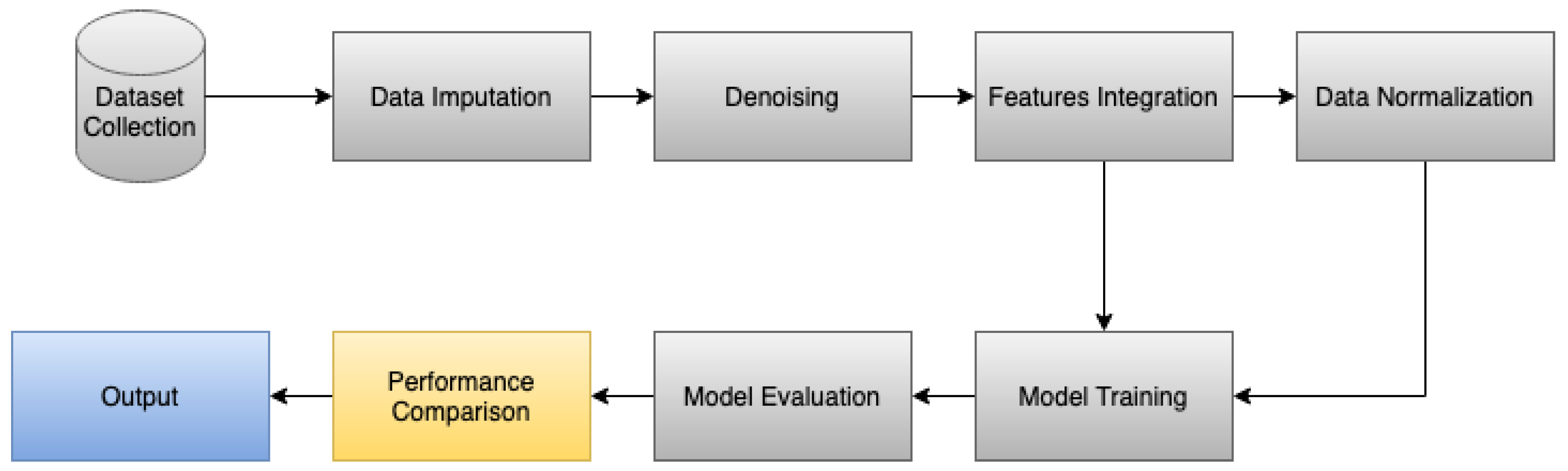
The methodology of this study proposes the automatic identification of five human activities, including walking, running, walking upstairs, walking downstairs, and standing. Figure 1 shows the flow diagram of the proposed methodology to perform the classification of the different samples with the extrapolation the missing samples before the classification of the data. The method is composed by seven modules, including data acquisition (Section 2.2), data imputation (Section 2.3), denoising (Section 2.4), features integration (Section 2.5), data normalization (Section 2.6), model training and evaluation (Section 2.7), and performance comparison (Section 2.8). These stages are explained in the next sections.
2.2. Study Participants and Data Acquisition
The data acquisition process is performed with non-intrusive equipment based on the use of a mobile device that incorporates different sensors, including an accelerometer, magnetometer, and gyroscope sensors. During the data acquisition, some failures may occur, and the missing samples were detected (Section 2.4). The data acquired includes the performance of different activities, including walking, running, standing, walking upstairs, and walking downstairs [22]. The different activities were performed and labeled by 25 individuals aged between 20 and 60 years old with different lifestyles and health states.
In general, the dataset is composed by 2000 captures of 5 s for each activity that corresponds to around 2.78 h of captures, representing 169.44 h of captures related to each activity. Thus, this dataset is composed by 13.9 h of captures shared by different individuals. The data were acquired using an Android application installed in a mobile device to record the mobile sensors data while performing the activities. All the participants kept the mobile phone in the front pocket of their pants while performing activities. The mobile device used is the BQ Aquaris 5.7 smartphone with a Quad Core CPU and 16 GB of internal memory [23]. Next, the data were used for the implementation of different techniques for data classification (Section 2.7). The mobile devices have different constraints related to the low memory, battery, and power processing, which may cause different failures [6,24]. After the acquisition, the original dataset without the application of the data imputation technique is available in [25], and the dataset with the application of the data imputation technique is available in [26].
2.3. Data Imputation
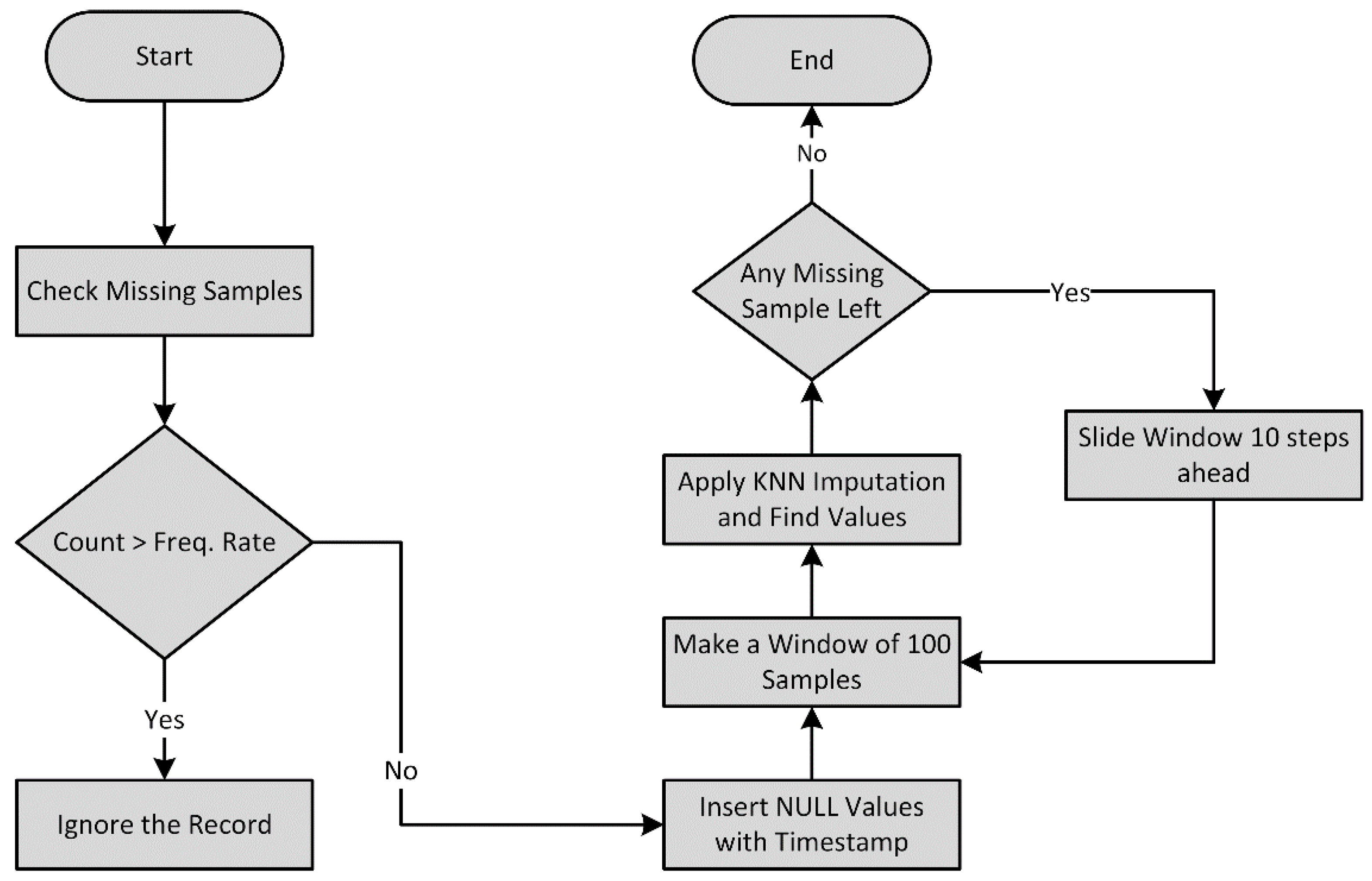
Once the dataset was collected, the next step was to analyze the missing samples and then extrapolate the missing samples using the data imputation technique. Figure 2 shows the flowchart for extrapolating the missing samples. It can the seen that the data imputation was performed in four major steps, which include missing samples identification, NULL values insertion, data segmentation, and data imputation.
2.3.1. Missing Samples Identification
After data acquisition and cleaning, the existence of missing samples in each record was performed. Regarding the training of the artificial intelligence methods, the existence of missing samples causes some impact in the correct recognition of human activities. It may occur by different reasons, including the user not performing an activity for a complete defined activity duration, failures of the sensors, environmental noise, or problems with the mobile device used for data acquisition.
Firstly, the number of missing samples in each record of the dataset was identified, analyzing the duration of each activity and the frequency rate of the sensors. The frequency rate differs from the sensors, where the frequency rate of the accelerometer and gyroscope was 100 Hz, and the frequency rate of the magnetometer was 10 Hz. Thus, the methods analyzed 500 samples for the accelerometer and magnetometer sensors, and 50 samples for the magnetometer sensor for each 5 s of activity.
Next, the number of missing samples for each capture was analyzed, excluding the samples that had less than 4 s of the data. Thus, the captures with more than 100 missing samples in the accelerometer and gyroscope sensors and the captures with more than 10 missing samples in the magnetometer sensor were discarded. This was done to be closer to the originality of the data than filling all synthetic samples to fulfill the space of missing samples.
From the above analysis, the missing samples count was identified with Equation (1).
Missing Samples Count = (Frequency rate × Activity Duration) − Samples Count in the Given Excerpt
Now, based upon the accelerometer and gyroscope specifications, Equations (1) and (2) were used, while in case of the magnetometer, Equations (1)–(3) were used:
Missing Samples Count for Acc. and Gy = (100 Hz × 5 s) − Samples Count in the Given Excerpt
Missing Samples Count for Acc. and Gy = 500 − Samples Count in the Given Excerpt
Missing Samples Count for Acc. and Gy = 500 − Samples Count in the Given Excerpt
Missing Samples Count for Magnetometer = (10 Hz × 5 s) − Samples Count in the Given Excerpt
Missing Samples Count for Magnetometer = 50 − Samples Count in the Given Excerpt.
Missing Samples Count for Magnetometer = 50 − Samples Count in the Given Excerpt.
2.3.2. NULL Values Insertion
After identifying the missing samples, the next step is to insert the NULL values to fill the space of the missing samples. Before inserting the NULL values, it was verified whether the missing samples count is greater than the sample frequency rate, i.e., the number of samples recorded in one second; then, the NULL values are not inserted, and the excerpt is ignored. Thus, if the missing samples count in each excerpt is more than 100 missing samples in case of the accelerometer and gyroscope or more than 10 missing samples in case of the magnetometer, then the excerpt is ignored. It is done to be closer to the originality of the data than filling all synthetic samples to fill the space of missing samples. On the other hand, if the missing samples count is less than or equal to the sample frequency rate, then NULL values are inserted after every constant time interval, i.e., after 1/100 s in case of an accelerometer and gyroscope and 1/10 s in case of a magnetometer, to fill the space of missing samples.
2.3.3. Data Segmentation
After filling the space of missing samples with NULL values, the segmentation of the samples was performed to apply the imputation technique to extrapolate the missing samples. The samples were segmented in each excerpt with respect to its sample frequency rate. In the case of the accelerometer and gyroscope, the samples were segmented into a window of 100 samples having 90 known samples and the first 10 unknown samples. While in the case of the magnetometer, the samples were segmented into a window of 10 samples having 9 known samples and one unknown sample. If the missing samples count was less than or equal to 10 in the case of the accelerometer and gyroscope, then all unknown samples were included with the known samples to make a window of 100 samples. While in case of the magnetometer, if the missing samples count was less than or equal to 2, all unknown samples were included with the known samples to make a window of 10 samples.
2.3.4. Data Imputation
The KNN imputation technique is a method to identify k samples in the used dataset by its similarity or closeness in the space [27]. The k samples are used to estimate the value of missing points. Generally, the value is imputed with the mean value of the k samples that are neighbors in the dataset.
Once the data were segmented, the KNN imputation technique was applied to extrapolate the missing samples. In the KNN imputation technique, we first found k-closest neighbors to the missing samples, and then these missing samples were imputed based upon the known k-closest neighbors. The data points having the shortest distance based on Euclidean distances were considered as the closest neighbors. The value of every missing sample was interpolated using the mean value of the k-closest neighbors. The missing samples count every time was noticed before applying the KNN imputation. If the missing samples count was less than 10, then the missing samples were filled in the first iteration. However, if the missing samples count was more than 10, then the window was moved 10 steps forward to make another chunk of data and apply the KNN imputation technique to extrapolate the missing samples. As shown in Figure 1, this process continued until all the missing samples were extrapolated.
In short, each recorded activity of the given dataset was analyzed, and the missing samples count was identified. Based upon the missing sample count, the comparison of the missing sample count with the sample frequency rate was performed. If the missing sample count is greater than the frequency rate of given excerpt, then that particular excerpt was ignored, and the next excerpt was analyzed. However, if the missing sample count is less than or equal to frequency rate, then the NULL values are inserted after a fixed time interval until all the missing sample are filled with the NULL values. Once the NULL values are inserted, then the samples were segmented into a window of 100 samples. Finally, the KNN imputation technique was applied for extrapolating the missing samples values based upon the known samples and this process was repeated as all the unknown values were extrapolated.
2.4. Denoising
The data cleaning process is important to remove the environment noise, effects of involuntary movements, and other artifacts, to improve the results of the recognition of human activities. According to the type of sensors used, the implemented method was the low-pass filter [28], which allows extracting features more clearly and is reliable for the implementation of classification methods.
2.5. Features Integration
After the data imputation, all three sensor excerpts of all datasets along with their activity labels were integrated to make a feature vector. The features extracted for each sensor are the five greatest distances between the maximum peaks, the average, standard deviation, variance, and median of the maximum peaks, and the standard deviation, average, maximum value, minimum value, variance, and median of the raw signal.
2.6. Data Normalization
After the extraction and integration of the different features, two different analyses were performed, i.e., one with raw features, and another one with the normalized features. According to the literature, there are different normalization techniques, but the most adapted to the implementation of the Deep Neural Networks (DNN) method with the DeepLearning4j framework [29] consists in the use of the mean and standard deviation [30].
2.7. Model Training and Evaluation
Once the feature vector was split into a training and test set, the deep learning model was trained over the training set for recognizing the human activities. After the extraction of the different features, the Deep Neural Networks (DNN) method was implemented with the DeepLearning4j framework [29]. During the hyper parameter tuning with a grid search approach [31], we considered the following values for each of the parameters: learning rate (100, 10−1, 10−2, 10−3, 10−3, 10−5, 10−6, 10−7) with an adaptive learning rate approach [32], number of hidden layers (1–4), regularization (L1, L2), normalization (min–max normalization), and mean and standard deviation. The following parameters were selected with the grid search and were configured for the final DNN model:
Finally, the evaluation of the performance of the trained model was performed, and it was tested over the unseen data, i.e., the test set. Note that the experiments were repeated five times with different seeds causing different training and test splits, as well as different initializations of the DNN network. During the experiments, the hyperparameters were fixed to the above values. Based upon the testing results, the confusion matrix was constructed, which is further used to evaluate the performance of the trained model with respect to different performance metrics. The results and metrics are discussed in Section 3, and they represent the averages of the five repetitions.
2.8. Performance Comparison
Since a data imputation technique was applied to extrapolate the missing samples, next, the evaluation of the effectiveness of the proposed data imputation technique was performed. For this purpose, the dataset was trained and tested with a deep learning algorithm first without data imputation. Afterwards, the dataset was trained and tested with the same deep learning model over the imputed dataset. Finally, the comparison of the performance of both the traditional approach and the proposed imputation approach was performed. The results of this experiment are discussed in Section 3.
3. Results
3.1. Data Imputation
This stage started with the identification of the number of missing samples. A sample rate of 100 Hz for the accelerometer and gyroscope sensors was considered, which corresponds to 500 samples per activity, and a sample rate of 10 Hz for the magnetometer sensor was considered, which corresponds to 50 samples per activity. Thus, as presented in Table 1, there are a lot of missing samples related to the accelerometer sensor. It shows the number of complete and missing values related to the accelerometer, where the same analysis was performed for the other sensors. The major number of missing samples was verified during walking upstairs.
Next, the data segmentation for the further implementation of data imputation techniques was performed. Table 2 shows an excerpt of accelerometer data during walking activity, where it is possible to observe that 50 samples of data are missing. Next, the frequency of 100 Hz was considered, and the values of the next 50 samples were measured. However, Table 3 shows the start of the process, filling the missing values in the missing rows as NULL. After all the missing values were filled as NULL, the data segmentation process was performed, as shown in Table 4. Finally, the KNN imputation method was implemented to extrapolate the NULL values, as shown in Table 5.
This technique is implemented for the files that have less than 100 missing samples in the case of the accelerometer and gyroscope and 10 missing samples in the case of the magnetometer. If more than 100 samples are missing, this capture should be discarded. Thus, the captures with more than 100 records missing from the accelerometer or gyroscope and the captures with more than 10 records missed from the magnetometer were ignored. The pattern of imputed data is similar to the other values in each capture, as explained in Section 2.
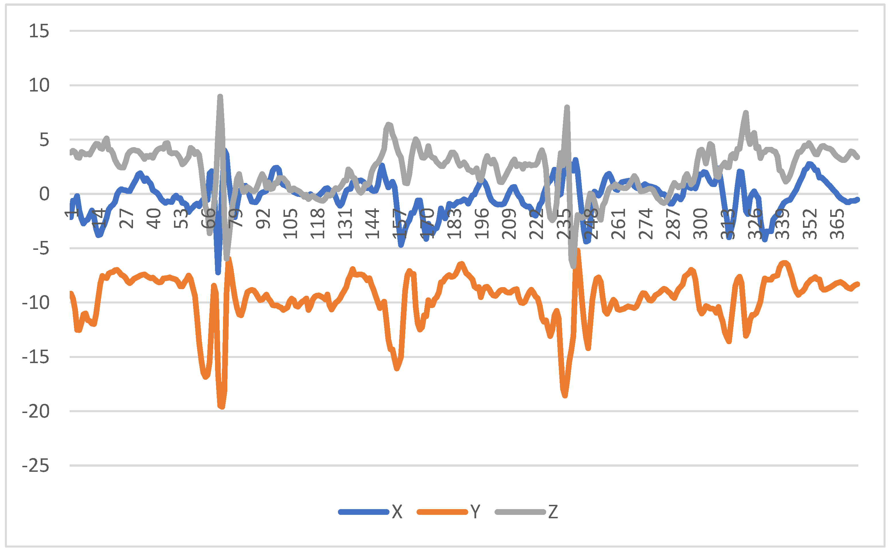
Next, Figure 3 shows the representation of the different axis of one capture during walking downstairs, where only 375 records are available. The number of records should be normalized to obtain reliable results in the data classification, i.e., all experiments must have 500 records. It is verified that 125 samples are missing. The KNN imputation method was implemented and the result is presented in Figure 4. However, the results obtained have the same pattern, but its amplitude is higher.
3.2. Data Classification
3.2.1. Non-Normalized Data
Considering the accelerometer data, the results obtained with non-imputed and non-normalized data are reported in the confusion matrix presented in Table 6. The implemented method reported an accuracy of 22.9%, a precision of 19.65%, a recall value of 22.9%, and an F1 score of 21.15%.
Considering the accelerometer and magnetometer sensors’ data, the results obtained with non-imputed and non-normalized data are reported in the confusion matrix presented in Table 7. The implemented method reported an accuracy of 40.69%, a precision of 56.4%, a recall value of 40.69%, and an F1 score of 47.27%.
Considering the accelerometer, magnetometer, and gyroscope sensors’ data, the results obtained with non-imputed and non-normalized data are reported in the confusion matrix presented in Table 8. The implemented method reported an accuracy of 74.46%, a precision of 78.24%, a recall value of 74.46%, and an F1 score of 76.3%.
Considering the accelerometer data, the results obtained with imputed and non-normalized data are reported in the confusion matrix presented in Table 9. The implemented method reported an accuracy of 20%, a precision of 20%, a recall value of 20%, and an F1 score of 20%.
Considering the accelerometer and magnetometer sensors’ data, the results obtained with imputed and non-normalized data are reported in the confusion matrix presented in Table 10. The implemented method reported an accuracy of 20.1%, a precision of 73.34%, a recall value of 20.1%, and an F1 score of 31.55%.
Considering the accelerometer, magnetometer, and gyroscope sensors’ data, the results obtained with imputed and non-normalized data are reported in the confusion matrix presented in Table 11. The implemented method reported an accuracy of 20.19%, a precision of 60.02%, a recall value of 20.19%, and an F1 score of 30.22%.
3.2.2. Normalized Data
Considering the accelerometer data, the results obtained with non-imputed and normalized data are reported in the confusion matrix presented in Table 12. The implemented method reported an accuracy of 85.89%, a precision of 86.21%, a recall value of 85.89%, and an F1 score of 86.05%.
Considering the accelerometer and magnetometer sensors’ data, the results obtained with non-imputed and normalized data are reported in the confusion matrix presented in Table 13. The implemented method reported an accuracy of 86.49%, a precision of 86.75%, a recall value of 86.49%, and an F1 score of 86.62%.
Considering the accelerometer, magnetometer, and gyroscope sensors’ data, the results obtained with non-imputed and normalized data are reported in the confusion matrix presented in Table 14. The implemented method reported an accuracy of 89.52%, a precision of 89.74%, a recall value of 89.51%, and an F1 score of 89.62%.
Considering the accelerometer data, the results obtained with imputed and normalized data are reported in the confusion matrix presented in Table 15. The implemented method reported an accuracy of 94.56%, a precision of 94.63%, a recall value of 94.56%, and an F1 score of 94.59%.
Considering the accelerometer and magnetometer sensors’ data, the results obtained with imputed and normalized data are reported in the confusion matrix presented in Table 16. The implemented method reported an accuracy of 98.24%, a precision of 98.28%, a recall value of 98.24%, and an F1 score of 98.26%.
Considering the accelerometer, magnetometer, and gyroscope sensors’ data, the results obtained with imputed and normalized data are reported in the confusion matrix presented in Table 17. The implemented method reported an accuracy of 99.82%, a precision of 99.82%, a recall value of 99.82%, and an F1 score of 99.82%.
4. Discussion
Table 18 summarizes the results obtained after all previously discussed experiments. Thus, 12 different experiments with respect to the different combinations of sensors and tests were used to analyze the effect of data imputation and data normalization, along with different combinations of sensors, as illustrated in Table 18. These results are presented in Figure 5, Figure 6 and Figure 7, based on the sensors combinations, i.e., accelerometer (Ac) only, accelerometer and magnetometer (Ac + Mg), and accelerometer, magnetometer and gyroscope (Ac + Mg + Gy).
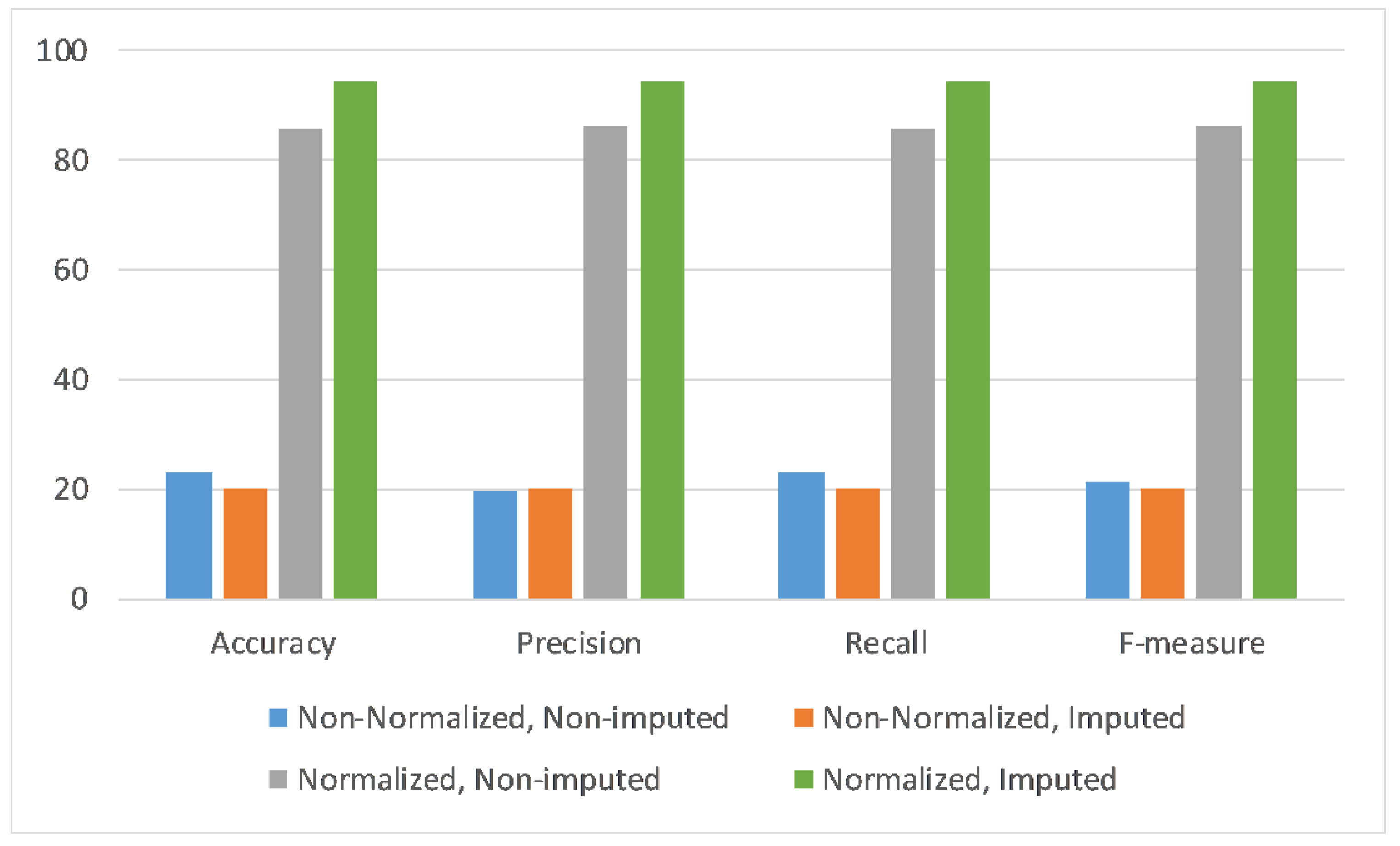
In Figure 5, only accelerometer sensor data are utilized to perform the experiments with respect to four scenarios of data normalization and data imputation combinations. Each scenario is evaluated across four performance metrics, i.e., accuracy, precision, recall, and F-measure. It can be observed that the deep learning model performance across all metrics is highest with the application of normalization and imputation on the given dataset.
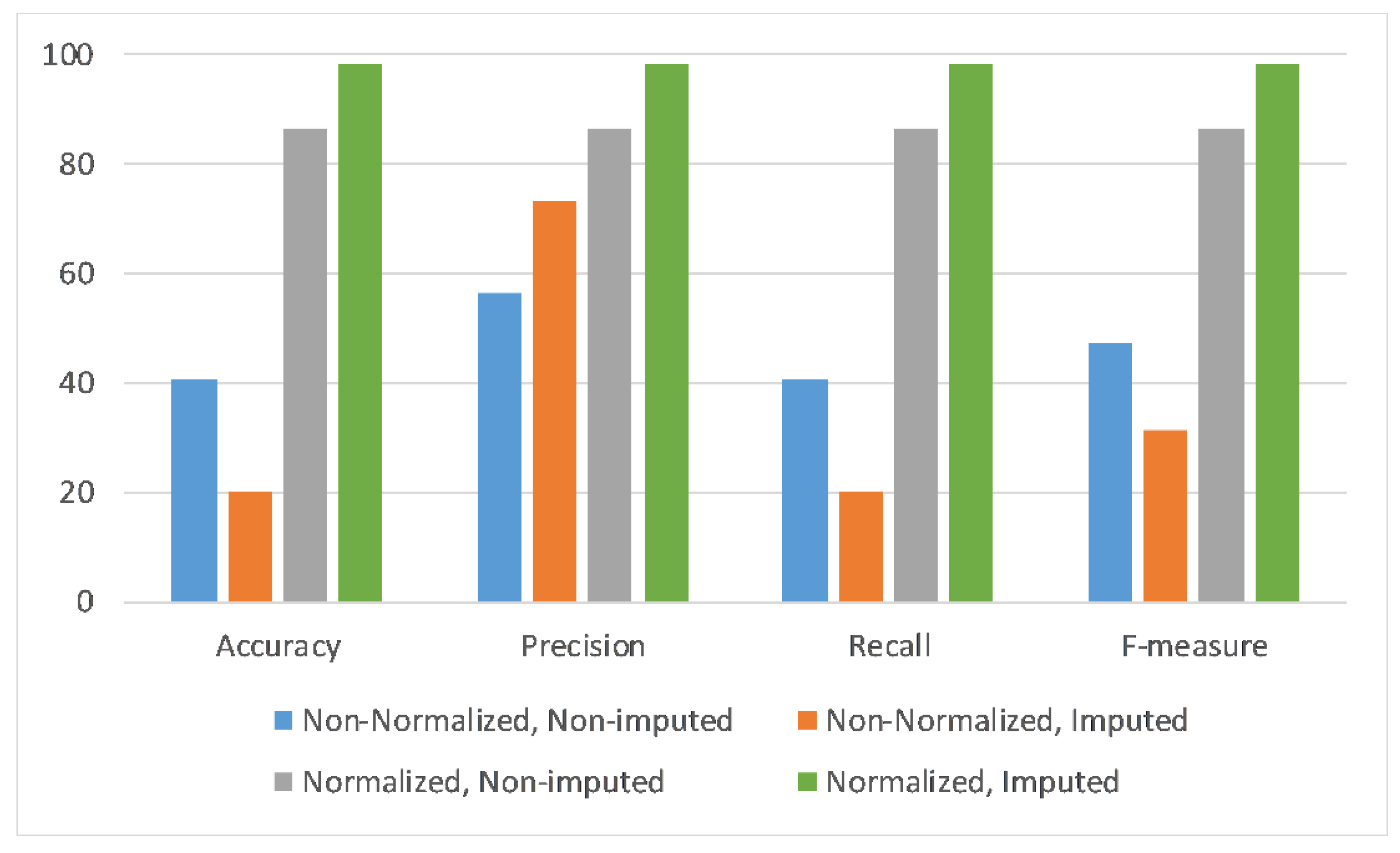
Similarly, Figure 6 shows the results when utilizing the accelerometer and magnetometer (Ac + Mg) sensors values to test the trained deep learning model with respect to four scenarios of data normalization and data imputation combinations. Each scenario is evaluated across four performance metrics, i.e., accuracy, precision, recall, and F-measure. It can be noticed that the deep learning model performance across all metrics is highest with the application of normalization and imputation on the given dataset.
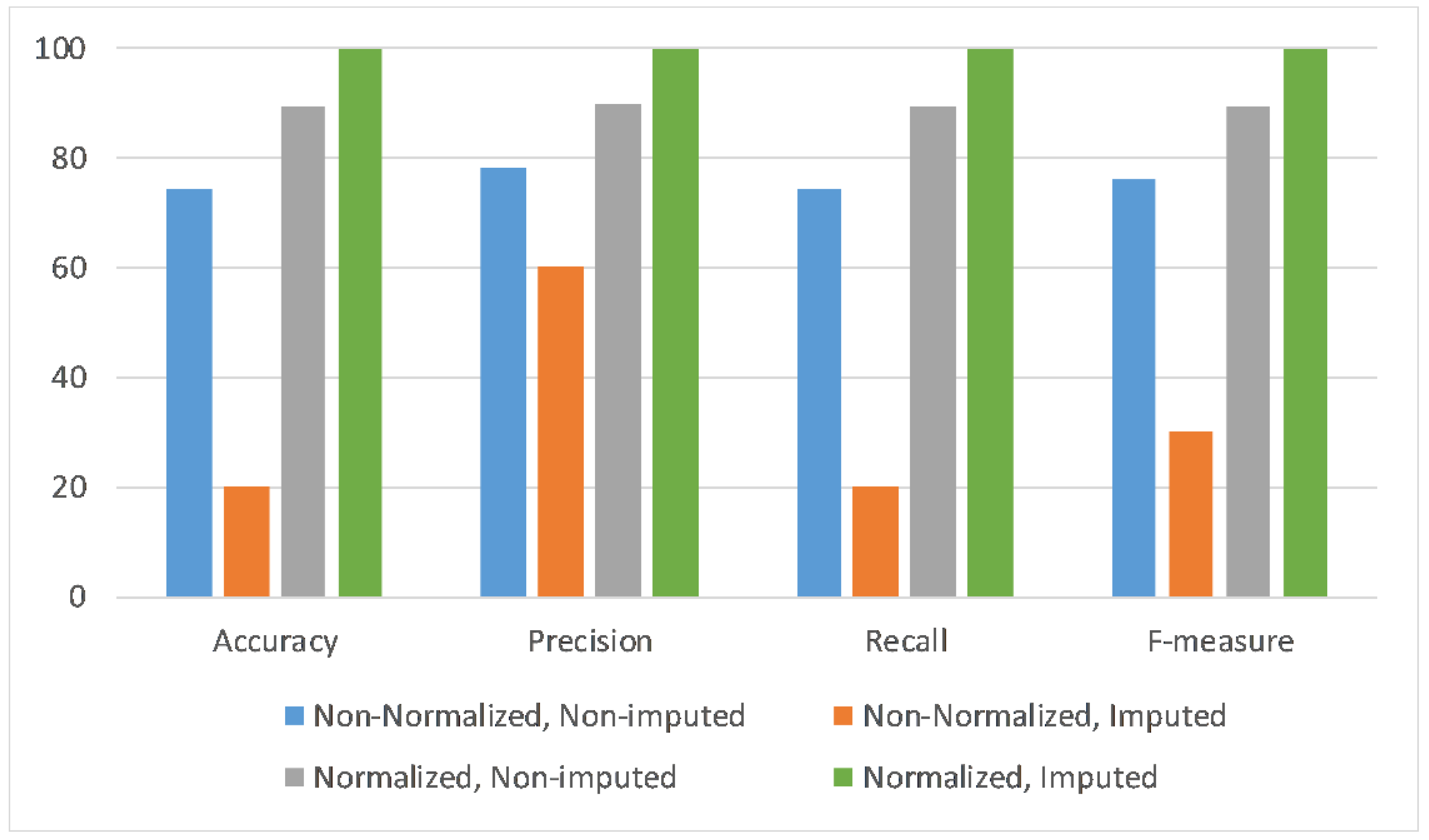
Likewise, Figure 7 displays the results when utilizing all three sensors data—i.e., accelerometer, magnetometer, and gyroscope—to test the trained deep learning model with respect to four scenarios of data normalization and data imputation combinations. Each scenario is evaluated across four performance metrics, i.e., accuracy, precision, recall, and F-measure. It can be observed that the deep learning model performance across all metrics is highest with the application of normalization and imputation on the given dataset.
As results of this study, it was verified that the pattern of the imputed data is similar to the original data. However, its frequency and amplitude are higher than in the original data. Regarding the data classification, depending on the number of sensors, the accuracy was between 22.9% and 74.46% for non-normalized data, and between 85.89% and 89.51% for normalized data. After the data imputation process, depending on the number of sensors, the accuracy changed to between 20.00% and 20.19% for non-normalized data, and between 94.56% and 99.82% for normalized data.
In summary, all the experimental results depict that the deep learning model better distinguishes daily living activities when both data normalization and data imputation techniques were applied. Moreover, the deep learning model gives the best results when imputed and normalized data from the combination of all three sensors are used, i.e., the accelerometer, magnetometer, and gyroscope. Furthermore, the use of data imputation reported an improvement of 25.36% in accuracy, 21.58% in precision, 25.36% in recall, and 23.52% in F-measure values over the normalized and imputed dataset across all three sensors, as compared to the non-normalized and non-imputed dataset across all three sensors. Therefore, from the above experimental results, it is verified that the performance of the deep learning model significantly increased when normalization and imputation techniques were applied to the dataset across all three sensors.
As we are using a proprietary dataset, the results are not comparable with others. However, several limitations were found that are related to the acquisition and positioning of the mobile device, the power processing of the methods implemented, and other involuntary limitations of the study [6,24].
The results obtained are affected by the reduced sample size. Initially, the data normalization was performed, and the maximum accuracy was around 89.51% [34,35] with the recognition of the same activities and with the use of the same sensors of this study. The implementation of imputation techniques increased the results with a maximum accuracy of 100%. Thus, we can conclude that the data imputation techniques increased the different results.
5. Conclusions
The missing samples in the dataset affect the performance of deep learning models. Therefore, in this paper, a methodology was proposed to extrapolate the missing samples of human activity recognition dataset captures to make deep models better classify the human daily living activities. The proposed methodology utilizes the K-Nearest Neighbors (KNN) imputation technique to extrapolate the missing samples in dataset captures. Thus, 12 experiments were performed to analyze the effect of data imputation and data normalization, along with different combinations of sensors.
The proposed methodology, when compared to a non-normalized and non-imputed dataset across all three sensors, reported an improvement of 25.36% in accuracy, 21.58% in precision, 25.36% in recall, and 23.52% in F-measure values over the normalized and imputed dataset across all three sensors. The experimental results revealed that the performance of the implemented model increased with the implementation of the data imputation method.
Author Contributions
Conceptualization, methodology, software, validation, formal analysis, investigation, writing—original draft preparation, writing—review and editing, I.M.P., F.H., N.M.G. and E.Z. All authors have read and agreed to the published version of the manuscript.
Funding
This work is funded by FCT/MEC through national funds and co-funded by FEDER—PT2020 partnership agreement under the project UIDB/EEA/50008/2020 (Este trabalho é financiado pela FCT/MEC através de fundos nacionais e cofinanciado pelo FEDER, no âmbito do Acordo de Parceria PT2020 no âmbito do projeto UIDB/EEA/50008/2020).
Acknowledgments
This work is funded by FCT/MEC through national funds and co-funded by FEDER—PT2020 partnership agreement under the project UIDB/EEA/50008/2020 (Este trabalho é financiado pela FCT/MEC através de fundos nacionais e cofinanciado pelo FEDER, no âmbito do Acordo de Parceria PT2020 no âmbito do projeto UIDB/EEA/50008/2020). This article is based upon work from COST Action IC1303–AAPELE–Architectures, Algorithms and Protocols for Enhanced Living Environments and COST Action CA16226–SHELD-ON–Indoor living space improvement: Smart Habitat for the Elderly, supported by COST (European Cooperation in Science and Technology). More information in www.cost.eu.
Conflicts of Interest
The authors declare no conflict of interest.
References
- Steele, R. Social media, mobile devices and sensors: Categorizing new techniques for health communication. In Proceedings of the 2011 Fifth International Conference on Sensing Technology, Palmerston North, New Zealand, 28 November–1 December 2011; pp. 187–192. [Google Scholar]
- Sousa, P.S.; Sabugueiro, D.; Felizardo, V.; Couto, R.; Pires, I.; Garcia, N.M. mHealth Sensors and Applications for Personal Aid. In Mobile Health; Adibi, S., Ed.; Springer Series in Bio-/Neuroinformatics; Springer International Publishing: Cham, Switzerland, 2015; Volume 5, pp. 265–281. ISBN 978-3-319-12816-0. [Google Scholar]
- Ferreira, J.M.; Pires, I.M.; Marques, G.; García, N.M.; Zdravevski, E.; Lameski, P.; Flórez-Revuelta, F.; Spinsante, S.; Xu, L. Activities of Daily Living and Environment Recognition Using Mobile Devices: A Comparative Study. Electronics 2020, 9, 180. [Google Scholar] [CrossRef] [Green Version]
- Seneviratne, S.; Hu, Y.; Nguyen, T.; Lan, G.; Khalifa, S.; Thilakarathna, K.; Hassan, M.; Seneviratne, A. A Survey of Wearable Devices and Challenges. IEEE Commun. Surv. Tutor. 2017, 19, 2573–2620. [Google Scholar] [CrossRef]
- Dimitrievski, A.; Zdravevski, E.; Lameski, P.; Trajkovik, V. A survey of Ambient Assisted Living systems: Challenges and opportunities. In Proceedings of the 2016 IEEE 12th International Conference on Intelligent Computer Communication and Processing (ICCP), Cluj-Napoca, Romania, 8–10 September 2016; pp. 49–53. [Google Scholar]
- Pires, I.; Felizardo, V.; Pombo, N.; Garcia, N.M. Limitations of energy expenditure calculation based on a mobile phone accelerometer. In Proceedings of the 2017 International Conference on High Performance Computing & Simulation (HPCS), Genoa, Italy, 17–21 July 2017; pp. 124–127. [Google Scholar]
- Cardinale, M.; Varley, M.C. Wearable Training-Monitoring Technology: Applications, Challenges, and Opportunities. Int. J. Sports Physiol. Perform. 2017, 12, S255–S262. [Google Scholar] [CrossRef] [PubMed] [Green Version]
- Pires, I.M.; Marques, G.; Garcia, N.M.; Pombo, N.; Flórez-Revuelta, F.; Spinsante, S.; Teixeira, M.C.; Zdravevski, E. Recognition of Activities of Daily Living and Environments Using Acoustic Sensors Embedded on Mobile Devices. Electronics 2019, 8, 1499. [Google Scholar] [CrossRef] [Green Version]
- Ling, W.; Dong-Mei, F. Estimation of Missing Values Using a Weighted K-Nearest Neighbors Algorithm. In Proceedings of the 2009 International Conference on Environmental Science and Information Application Technology, Wuhan, China, 4–5 July 2009; pp. 660–663. [Google Scholar]
- Costa, S.E.P.; Rodrigues, J.J.P.C.; Silva, B.M.C.; Isento, J.N.; Corchado, J.M. Integration of Wearable Solutions in AAL Environments with Mobility Support. J. Med. Syst. 2015, 39, 184. [Google Scholar] [CrossRef] [PubMed]
- Vateekul, P.; Sarinnapakorn, K. Tree-Based Approach to Missing Data Imputation. In Proceedings of the 2009 IEEE International Conference on Data Mining Workshops, Miami, FL, USA, 6 December 2009; pp. 70–75. [Google Scholar]
- D’Ambrosio, A.; Aria, M.; Siciliano, R. Accurate Tree-based Missing Data Imputation and Data Fusion within the Statistical Learning Paradigm. J. Classif. 2012, 29, 227–258. [Google Scholar] [CrossRef]
- Ni, D.; Leonard, J.D.; Guin, A.; Feng, C. Multiple Imputation Scheme for Overcoming the Missing Values and Variability Issues in ITS Data. J. Transp. Eng. 2005, 131, 931–938. [Google Scholar] [CrossRef] [Green Version]
- Smith, B.L.; Scherer, W.T.; Conklin, J.H. Exploring Imputation Techniques for Missing Data in Transportation Management Systems. Transp. Res. Rec. 2003, 1836, 132–142. [Google Scholar] [CrossRef]
- Qu, L.; Zhang, Y.; Hu, J.; Jia, L.; Li, L. A BPCA based missing value imputing method for traffic flow volume data. In Proceedings of the 2008 IEEE Intelligent Vehicles Symposium, Eindhoven, The Netherlands, 4–6 June 2008; pp. 985–990. [Google Scholar]
- Jiang, N.; Gruenwald, L. Estimating Missing Data in Data Streams. In Advances in Databases: Concepts, Systems and Applications; Lecture Notes in Computer Science; Kotagiri, R., Krishna, P.R., Mohania, M., Nantajeewarawat, E., Eds.; Springer: Berlin/Heidelberg, Germany, 2007; Volume 4443, pp. 981–987. ISBN 978-3-540-71702-7. [Google Scholar]
- Guo, Q.; Liu, B.; Chen, C.W. A two-layer and multi-strategy framework for human activity recognition using smartphone. In Proceedings of the 2016 IEEE International Conference on Communications (ICC), Kuala Lumpur, Malaysia, 23–27 May 2016; pp. 1–6. [Google Scholar]
- Shoaib, M.; Scholten, H.; Havinga, P.J.M. Towards Physical Activity Recognition Using Smartphone Sensors. In Proceedings of the 2013 IEEE 10th International Conference on Ubiquitous Intelligence and Computing and 2013 IEEE 10th International Conference on Autonomic and Trusted Computing, Vietri sul Mere, Italy, 18–21 December 2013; pp. 80–87. [Google Scholar]
- Elhoushi, M.; Georgy, J.; Wahdan, A.; Korenberg, M.; Noureldin, A. Using portable device sensors to recognize height changing modes of motion. In Proceedings of the 2014 IEEE International Instrumentation and Measurement Technology Conference (I2MTC) Proceedings, Montevideo, Uruguay, 12–15 May 2014; pp. 477–481. [Google Scholar]
- Ronao, C.A.; Cho, S.-B. Human activity recognition using smartphone sensors with two-stage continuous hidden Markov models. In Proceedings of the 2014 10th International Conference on Natural Computation (ICNC), Xiamen, China, 19–21 August 2014; pp. 681–686. [Google Scholar]
- Zdravevski, E.; Risteska Stojkoska, B.; Standl, M.; Schulz, H. Automatic machine-learning based identification of jogging periods from accelerometer measurements of adolescents under field conditions. PLoS ONE 2017, 12, e0184216. [Google Scholar] [CrossRef] [PubMed]
- Pires, I.M. Available online: https://github.com/impires/August_2017-_Multi-sensor_data_fusion_in_mobile_devices_for_the_identification_of_activities_of_dail (accessed on 8 May 2020).
- Smartphones, B.Q. Aquaris|BQ Portugal. Available online: https://www.bq.com/pt/smartphones (accessed on 29 August 2020).
- Pires, I.M.; Garcia, N.M.; Pombo, N.; Flórez-Revuelta, F. Limitations of the Use of Mobile Devices and Smart Environments for the Monitoring of Ageing People. In Proceedings of the HSP 2018, Strasbourg, France, 17 May 2018. [Google Scholar]
- Pires, I.; Garcia, N.M. Raw Dataset with Accelerometer, Gyroscope and Magnetometer Data for Activities with Motion. Mendeley Data 2020, 1. [Google Scholar] [CrossRef]
- Pires, I. Imputed Dataset with Accelerometer, Gyroscope and Magnetometer Data for Activities with Motion. Mendeley Data 2020, 1. [Google Scholar] [CrossRef]
- Beretta, L.; Santaniello, A. Nearest neighbor imputation algorithms: A critical evaluation. BMC Med. Inform. Decis. Mak. 2016, 16. [Google Scholar] [CrossRef] [PubMed] [Green Version]
- Graizer, V. Effect of low-pass filtering and re-sampling on spectral and peak ground acceleration in strong-motion records. In Proceedings of the 15th World Conference of Earthquake Engineering, Lisbon, Portugal, 24–28 September 2012; pp. 24–28. [Google Scholar]
- Deeplearning4j. Available online: https://deeplearning4j.org/ (accessed on 2 August 2020).
- Brocca, L.; Melone, F.; Moramarco, T.; Wagner, W.; Naeimi, V.; Bartalis, Z.; Hasenauer, S. Improving runoff prediction through the assimilation of the ASCAT soil moisture product. Hydrol. Earth Syst. Sci. 2010, 14, 1881–1893. [Google Scholar] [CrossRef] [Green Version]
- Lameski, P.; Zdravevski, E.; Mingov, R.; Kulakov, A. SVM Parameter Tuning with Grid Search and Its Impact on Reduction of Model Over-fitting. In Rough Sets, Fuzzy Sets, Data Mining, and Granular Computing; Lecture Notes in Computer Science; Yao, Y., Hu, Q., Yu, H., Grzymala-Busse, J.W., Eds.; Springer International Publishing: Cham, Switzerland, 2015; Volume 9437, pp. 464–474. ISBN 978-3-319-25782-2. [Google Scholar]
- Petrovska, B.; Atanasova-Pacemska, T.; Corizzo, R.; Mignone, P.; Lameski, P.; Zdravevski, E. Aerial Scene Classification through Fine-Tuning with Adaptive Learning Rates and Label Smoothing. Appl. Sci. 2020, 10, 5792. [Google Scholar] [CrossRef]
- Ng, A.Y. Feature selection, L1 vs. L2 regularization, and rotational invariance. In Proceedings of the Twenty-First International Conference on Machine Learning—ICML ’04, Banff, AB, Canada, 4–8 July 2004; p. 78. [Google Scholar]
- Pires, I.M.; Garcia, N.M.; Pombo, N.; Flórez-Revuelta, F.; Spinsante, S.; Teixeira, M.C. Identification of activities of daily living through data fusion on motion and magnetic sensors embedded on mobile devices. Pervasive Mob. Comput. 2018, 47, 78–93. [Google Scholar] [CrossRef]
- Pires, I.M.; Marques, G.; Garcia, N.M.; Flórez-Revuelta, F.; Canavarro Teixeira, M.; Zdravevski, E.; Spinsante, S.; Coimbra, M. Pattern Recognition Techniques for the Identification of Activities of Daily Living Using a Mobile Device Accelerometer. Electronics 2020, 9, 509. [Google Scholar] [CrossRef] [Green Version]
Figure 1.
Workflow of the proposed methodology.

Figure 2.
Workflow of the data imputation scheme.

Figure 3.
Accelerometer sample related to moving downstairs.

Figure 4.
Imputed data for the accelerometer sample related to moving downstairs.

Figure 5.
Performance of deep learning model when utilizing only accelerometer data to classify the human daily living activities across four data normalization and data imputation scenarios.
Figure 5.
Performance of deep learning model when utilizing only accelerometer data to classify the human daily living activities across four data normalization and data imputation scenarios.

Figure 6.
Performance of deep learning model when utilizing accelerometer and magnetometer data to classify the human daily living activities across four data normalization and data imputation scenarios.
Figure 6.
Performance of deep learning model when utilizing accelerometer and magnetometer data to classify the human daily living activities across four data normalization and data imputation scenarios.

Figure 7.
Performance of deep learning model when utilizing accelerometer, magnetometer, and gyroscope data to classify the human daily living activities across four data normalization and data imputation scenarios.
Figure 7.
Performance of deep learning model when utilizing accelerometer, magnetometer, and gyroscope data to classify the human daily living activities across four data normalization and data imputation scenarios.


Table 1.
Analysis of missing samples from the accelerometer sensor.
| Activity | Total Records | Complete Records | Records with Missing Samples | ||
|---|---|---|---|---|---|
| ≤10 | >10 & ≤100 | >100 | |||
| Walking | 2000 | 1217 | 317 | 327 | 139 |
| Running | 2000 | 1513 | 403 | 72 | 12 |
| Standing | 2000 | 1601 | 360 | 37 | 2 |
| Walking upstairs | 2000 | 1293 | 173 | 115 | 419 |
| Walking downstairs | 2000 | 1636 | 111 | 75 | 178 |
Table 2.
Excerpt of accelerometer sample for walking activity.
| # | Timestamp | X | Y | Z |
|---|---|---|---|---|
| 1 | 1493996698893 | −2.145 | −9.174 | 3.802 |
| 2 | 1493996698902 | −0.612 | −9.625 | 3.984 |
| 3 | 1493996698914 | −0.641 | −10.678 | 3.84 |
| … | ||||
| 448 | 1493996702662 | −0.641 | −8.533 | 3.84 |
| 449 | 1493996702663 | −0.632 | −8.399 | 3.61 |
| 450 | 1493996702672 | −0.526 | −8.322 | 3.39 |
Table 3.
Excerpt of accelerometer sample for walking activity with missing samples filled as NULL.
| # | Timestamp | X | Y | Z |
|---|---|---|---|---|
| 450 | 1493996702672 | −0.526 | −8.322 | 3.39 |
| 451 | 1493996702682 | NULL | NULL | NULL |
| 452 | 1493996702692 | NULL | NULL | NULL |
| … | ||||
| 499 | 1493996703162 | NULL | NULL | NULL |
| 500 | 1493996703172 | NULL | NULL | NULL |
Table 4.
Data segmentation before applying the K-Nearest Neighbors (KNN) imputation technique.
| # | Timestamp | X | Y | Z |
|---|---|---|---|---|
| 441 | 1493996702582 | −0.526 | −8.322 | 3.39 |
| 442 | 1493996702593 | −0.392 | −8.102 | 3.208 |
| 443 | 1493996702604 | −0.507 | −8.207 | 3.112 |
| … | ||||
| 449 | 1493996702663 | −0.632 | −8.399 | 3.61 |
| 450 | 1493996702672 | −0.526 | −8.322 | 3.39 |
| 451 | 1493996702682 | NULL | NULL | NULL |
| 452 | 1493996702692 | NULL | NULL | NULL |
Table 5.
Missing samples filled after applying the KNN imputation technique.
| # | Timestamp | X | Y | Z |
|---|---|---|---|---|
| 449 | 1493996702663 | −0.632 | −8.399 | 3.61 |
| 450 | 1493996702672 | −0.526 | −8.322 | 3.39 |
| 451 | 1493996702682 | −0.329 | −9.866 | −1.05 |
| 452 | 1493996702692 | −0.332 | −9.197 | 2.405 |
Table 6.
Confusion matrix related to non-normalized and non-imputed data from the accelerometer sensor.
Table 6.
Confusion matrix related to non-normalized and non-imputed data from the accelerometer sensor.
| Predicted Class | ||||||
|---|---|---|---|---|---|---|
| Walking Downstairs | Walking Upstairs | Running | Standing | Walking | ||
| Actual Class | Walking Downstairs | 290 | 0 | 0 | 1709 | 1 |
| Walking Upstairs | 210 | 0 | 0 | 1790 | 0 | |
| Running | 3 | 1 | 0 | 1996 | 0 | |
| Standing | 0 | 0 | 0 | 2000 | 0 | |
| Walking | 1 | 0 | 0 | 1999 | 0 | |
Table 7.
Confusion matrix related to non-normalized and non-imputed data from the accelerometer and magnetometer sensors.
Table 7.
Confusion matrix related to non-normalized and non-imputed data from the accelerometer and magnetometer sensors.
| Predicted Class | ||||||
|---|---|---|---|---|---|---|
| Walking Downstairs | Walking Upstairs | Running | Standing | Walking | ||
| Actual Class | Walking Downstairs | 179 | 2 | 20 | 1791 | 8 |
| Walking Upstairs | 67 | 13 | 8 | 1912 | 0 | |
| Running | 1 | 0 | 1877 | 121 | 1 | |
| Standing | 0 | 0 | 0 | 2000 | 0 | |
| Walking | 4 | 0 | 2 | 1994 | 0 | |
Table 8.
Confusion matrix related to non-normalized and non-imputed data from the accelerometer, magnetometer, and gyroscope sensors.
Table 8.
Confusion matrix related to non-normalized and non-imputed data from the accelerometer, magnetometer, and gyroscope sensors.
| Predicted Class | ||||||
|---|---|---|---|---|---|---|
| Walking Downstairs | Walking Upstairs | Running | Standing | Walking | ||
| Actual Class | Walking Downstairs | 99 | 1534 | 2 | 5 | 360 |
| Walking Upstairs | 31 | 1618 | 0 | 7 | 344 | |
| Running | 0 | 38 | 1879 | 29 | 54 | |
| Standing | 0 | 14 | 0 | 1986 | 0 | |
| Walking | 1 | 80 | 0 | 55 | 1864 | |
Table 9.
Confusion matrix related to non-normalized and imputed data from the accelerometer sensor.
| Predicted Class | ||||||
|---|---|---|---|---|---|---|
| Walking Downstairs | Walking Upstairs | Running | Standing | Walking | ||
| Actual Class | Walking Downstairs | 0 | 0 | 2000 | 0 | 0 |
| Walking Upstairs | 0 | 0 | 2000 | 0 | 0 | |
| Running | 0 | 0 | 2000 | 0 | 0 | |
| Standing | 0 | 0 | 2000 | 0 | 0 | |
| Walking | 0 | 0 | 2000 | 0 | 0 | |
Table 10.
Confusion matrix related to non-normalized and imputed data from the accelerometer and magnetometer sensors.
Table 10.
Confusion matrix related to non-normalized and imputed data from the accelerometer and magnetometer sensors.
| Predicted Class | ||||||
|---|---|---|---|---|---|---|
| Walking Downstairs | Walking Upstairs | Running | Standing | Walking | ||
| Actual Class | Walking Downstairs | 0 | 0 | 0 | 2000 | 0 |
| Walking Upstairs | 0 | 0 | 0 | 2000 | 0 | |
| Running | 0 | 0 | 5 | 1995 | 0 | |
| Standing | 0 | 0 | 0 | 2000 | 0 | |
| Walking | 0 | 0 | 0 | 1995 | 5 | |
Table 11.
Confusion matrix related to non-normalized and imputed data from the accelerometer, magnetometer, and gyroscope sensors.
Table 11.
Confusion matrix related to non-normalized and imputed data from the accelerometer, magnetometer, and gyroscope sensors.
| Predicted Class | ||||||
|---|---|---|---|---|---|---|
| Walking Downstairs | Walking Upstairs | Running | Standing | Walking | ||
| Actual Class | Walking Downstairs | 0 | 0 | 0 | 0 | 2000 |
| Walking Upstairs | 0 | 19 | 0 | 0 | 1981 | |
| Running | 0 | 0 | 0 | 0 | 2000 | |
| Standing | 0 | 0 | 0 | 0 | 2000 | |
| Walking | 0 | 0 | 0 | 0 | 2000 | |
Table 12.
Confusion matrix related to normalized and non-imputed data from the accelerometer sensor.
Table 12.
Confusion matrix related to normalized and non-imputed data from the accelerometer sensor.
| Predicted Class | ||||||
|---|---|---|---|---|---|---|
| Walking Downstairs | Walking Upstairs | Running | Standing | Walking | ||
| Actual Class | Walking Downstairs | 1334 | 510 | 9 | 4 | 143 |
| Walking Upstairs | 230 | 1639 | 4 | 14 | 113 | |
| Running | 20 | 34 | 1909 | 9 | 28 | |
| Standing | 0 | 11 | 0 | 1985 | 4 | |
| Walking | 109 | 128 | 9 | 32 | 1722 | |
Table 13.
Confusion matrix related to non-normalized and imputed data from the accelerometer and magnetometer sensors.
Table 13.
Confusion matrix related to non-normalized and imputed data from the accelerometer and magnetometer sensors.
| Predicted Class | ||||||
|---|---|---|---|---|---|---|
| Walking Downstairs | Walking Upstairs | Running | Standing | Walking | ||
| Actual Class | Walking Downstairs | 1359 | 455 | 2 | 13 | 171 |
| Walking Upstairs | 214 | 1631 | 1 | 18 | 136 | |
| Running | 20 | 32 | 1914 | 26 | 8 | |
| Standing | 1 | 12 | 0 | 1984 | 3 | |
| Walking | 60 | 125 | 1 | 53 | 1761 | |
Table 14.
Confusion matrix related to normalized and non-imputed data from the accelerometer, magnetometer, and gyroscope sensors.
Table 14.
Confusion matrix related to normalized and non-imputed data from the accelerometer, magnetometer, and gyroscope sensors.
| Predicted Class | ||||||
|---|---|---|---|---|---|---|
| Walking Downstairs | Walking Upstairs | Running | Standing | Walking | ||
| Actual Class | Walking Downstairs | 1545 | 325 | 1 | 3 | 126 |
| Walking Upstairs | 204 | 1684 | 1 | 5 | 106 | |
| Running | 5 | 46 | 1917 | 21 | 11 | |
| Standing | 0 | 13 | 0 | 1987 | 0 | |
| Walking | 19 | 118 | 2 | 43 | 1818 | |
Table 15.
Confusion matrix related to normalized and non-imputed data from the accelerometer sensor.
Table 15.
Confusion matrix related to normalized and non-imputed data from the accelerometer sensor.
| Predicted Class | ||||||
|---|---|---|---|---|---|---|
| Walking Downstairs | Walking Upstairs | Running | Standing | Walking | ||
| Actual Class | Walking Downstairs | 1883 | 117 | 0 | 0 | 0 |
| Walking Upstairs | 84 | 1787 | 0 | 14 | 115 | |
| Running | 4 | 18 | 1946 | 0 | 32 | |
| Standing | 0 | 6 | 0 | 1989 | 5 | |
| Walking | 12 | 130 | 7 | 0 | 1851 | |
Table 16.
Confusion matrix related to normalized and imputed data from the accelerometer and magnetometer sensors.
Table 16.
Confusion matrix related to normalized and imputed data from the accelerometer and magnetometer sensors.
| Predicted Class | ||||||
|---|---|---|---|---|---|---|
| Walking Downstairs | Walking Upstairs | Running | Standing | Walking | ||
| Actual Class | Walking Downstairs | 2000 | 0 | 0 | 0 | 0 |
| Walking Upstairs | 0 | 2000 | 0 | 0 | 0 | |
| Running | 14 | 9 | 1959 | 0 | 18 | |
| Standing | 0 | 0 | 0 | 2000 | 0 | |
| Walking | 34 | 86 | 15 | 0 | 1865 | |
Table 17.
Confusion matrix related to normalized and imputed data from the accelerometer, magnetometer, and gyroscope sensors.
Table 17.
Confusion matrix related to normalized and imputed data from the accelerometer, magnetometer, and gyroscope sensors.
| Predicted Class | ||||||
|---|---|---|---|---|---|---|
| Walking Downstairs | Walking Upstairs | Running | Standing | Walking | ||
| Actual Class | Walking Downstairs | 2000 | 0 | 0 | 0 | 0 |
| Walking Upstairs | 0 | 2000 | 0 | 0 | 0 | |
| Running | 0 | 18 | 1982 | 0 | 0 | |
| Standing | 0 | 0 | 0 | 2000 | 0 | |
| Walking | 0 | 0 | 0 | 0 | 2000 | |
Table 18.
Summarized results of all previous experiments.
| Scenario | Sensors | Accuracy | Precision | Recall | F-Measure |
|---|---|---|---|---|---|
| Non-Normalized, Non-imputed | Ac | 22.9 | 19.65 | 22.9 | 21.15 |
| Ac + Mg | 40.69 | 56.4 | 40.69 | 47.27 | |
| Ac + Mg + Gy | 74.46 | 78.24 | 74.46 | 76.3 | |
| Non-Normalized, Imputed | Ac | 20 | 20 | 20 | 20 |
| Ac + Mg | 20.1 | 73.34 | 20.1 | 31.55 | |
| Ac + Mg + Gy | 20.19 | 60.02 | 20.19 | 30.22 | |
| Normalized, Non-imputed | Ac | 85.89 | 86.21 | 85.89 | 86.05 |
| Ac + Mg | 86.49 | 86.75 | 86.49 | 86.62 | |
| Ac + Mg + Gy | 89.52 | 89.74 | 89.51 | 89.62 | |
| Normalized, Imputed | Ac | 94.56 | 94.63 | 94.56 | 94.59 |
| Ac + Mg | 98.24 | 98.28 | 98.24 | 98.26 | |
| Ac + Mg + Gy | 99.82 | 99.82 | 99.82 | 99.82 |
© 2020 by the authors. Licensee MDPI, Basel, Switzerland. This article is an open access article distributed under the terms and conditions of the Creative Commons Attribution (CC BY) license (http://creativecommons.org/licenses/by/4.0/).
Share and Cite
MDPI and ACS Style
Pires, I.M.; Hussain, F.; Garcia, N.M.; Zdravevski, E. Improving Human Activity Monitoring by Imputation of Missing Sensory Data: Experimental Study. Future Internet 2020, 12, 155. https://0-doi-org.brum.beds.ac.uk/10.3390/fi12090155
AMA Style
Pires IM, Hussain F, Garcia NM, Zdravevski E. Improving Human Activity Monitoring by Imputation of Missing Sensory Data: Experimental Study. Future Internet. 2020; 12(9):155. https://0-doi-org.brum.beds.ac.uk/10.3390/fi12090155
Chicago/Turabian StylePires, Ivan Miguel, Faisal Hussain, Nuno M. Garcia, and Eftim Zdravevski. 2020. "Improving Human Activity Monitoring by Imputation of Missing Sensory Data: Experimental Study" Future Internet 12, no. 9: 155. https://0-doi-org.brum.beds.ac.uk/10.3390/fi12090155
Note that from the first issue of 2016, this journal uses article numbers instead of page numbers. See further details here.