Portfolio Learning Based on Deep Learning


School of Computer Engineering and Science, Shanghai University, Shanghai 200444, China
*
Author to whom correspondence should be addressed.
Future Internet 2020, 12(11), 202; https://0-doi-org.brum.beds.ac.uk/10.3390/fi12110202
Submission received: 30 October 2020
/
Revised: 13 November 2020
/
Accepted: 15 November 2020
/
Published: 18 November 2020
(This article belongs to the Collection Computer Vision, Deep Learning and Machine Learning with Applications)
Abstract
:Traditional portfolio theory divides stocks into different categories using indicators such as industry, market value, and liquidity, and then selects representative stocks according to them. In this paper, we propose a novel portfolio learning approach based on deep learning and apply it to China’s stock market. Specifically, this method is based on the similarity of deep features extracted from candlestick charts. First, we obtained whole stock information from Tushare, a professional financial data interface. These raw time series data are then plotted into candlestick charts to make an image dataset for studying the stock market. Next, the method extracts high-dimensional features from candlestick charts through an autoencoder. After that, K-means is used to cluster these high-dimensional features. Finally, we choose one stock from each category according to the Sharpe ratio and a low-risk, high-return portfolio is obtained. Extensive experiments are conducted on stocks in the Chinese stock market for evaluation. The results demonstrate that the proposed portfolio outperforms the market’s leading funds and the Shanghai Stock Exchange Composite Index (SSE Index) in a number of metrics.
1. Introduction
Quantitative trading [1] has gradually become the main trading method in mature capital markets. With the rise of deep learning over the years, more and more people have applied it to capital markets. Portfolio learning is an important area in quantitative trading. However, current mainstream methods can only handle numerical data. This article proposes an image-based portfolio learning strategy using CNN.
How to make reasonable investment decisions has always been an important research field in quantitative trading and behavioral finance [2]. Stock technical analysis theory believes that all market news will be reflected in the stock price, and stocks that have similar responses to the news are more similar. The candlestick charts are useful tools to describe stock price fluctuations. A candlestick chart is a kind of financial chart that includes the lowest, highest, opening, and closing prices. It can effectively reflect stocks’ fluctuation, and is the most important analysis object of the technical analysis theory in the securities market. Thus, we use candlestick charts’ similarity to measure stocks’ similarity. We then try to find a group of low-similarity stocks based on the candlestick chart. This is because investment portfolios and asset weights should be constructed and optimized to maximize the Sharpe ratio [3], which is defined as the ratio of return to risk.
In mean-variance theory [4], a classic modern portfolio theory, mean and variance are used to assess the return and the risk of stocks, respectively. The theory posits that stocks with the least risk should be selected at the same rate of return. In addition, stocks of lower correlation coefficients should be considered. We reduce non-system risk of the portfolio through investment diversification. How to choose a set of stocks with high return and the low a correlation coefficient while measuring stock similarity is particularly important.
However, most similarity assessments have the following problems: (1) Typically, time series are used to measure similarity through a linear metric, such as co-variance and Pearson. However, these metrics can only reflect the linear characteristics of stock fluctuations. (2) Data from the past n days is needed to estimate the co-variance, which may not describe the whole market well. In order to solve these problems, we propose a method for estimating similarity using features extracted by deep learning.
There have been a number of successful deep learning works in image processing. For example, the Convolutional Autoeocoder (CAE) [5] and Bidirectional Generative Adversarial Networks (BiGANs) [6] have achieved good results in image analysis. Amodei [7] converts a 1D signal into a spectrogram (i.e., an image) in order to leverage the strength of CNNs to achieve promising recognition performance. Deep Q-network (DQN) [8] takes in images from Atari games as state representations, makes a decision based on state, and has beat the best human player in many games. For the same motivation, we explored the conversion of a four-channel stock time series (the lowest, highest, open, and close prices) to the candlestick chart, presenting the price history in the form of an image. In order to achieve end-to-end learning, we chose an unsupervised CAE to learn stock features from candlestick charts.
Therefore, the first innovation of this study is to use deep neural networks to encode candlestick charts into deep features. Compared with raw time series, deep feature extracted from candlestick charts can better reflect high-level information such as nonlinear trends and the semantics of stock movements. In addition, we propose a new method using image information for investment decision-making. Although some deep learning models, such as Long Short-Term Memory (LSTM) [9] and Recurrent Neural Network (RNN) [10], have been applied to optimize the portfolio [11,12], they extract deep features from raw time series rather than candlestick charts for investment decision-making.
We built a new end-to-end model to obtain a portfolio. Steps include: (1) Using CAE to learn deep features from candlestick charts; (2) clustering the deep features, thus dividing all stocks in the market into clusters; (3) building a portfolio based on the clustering of the market. For visual representation learning, we made a dataset of 600 k candlestick charts and input them into CAE for feature learning. In the following clustering, deep features are used for similarity matching.
2. Related Work
Applying deep learning to portfolio selection has attracted a lot of attention from researchers, and many efforts have been dedicated to apply deep convolution networks to portfolio selection. Andrea Loreggia [13] presented an automated methodology for producing an informative set of features utilizing a deep neural network. El-Yaniv [14] and Borodin et al. [15] surveyed the portfolio selection problem in the framework of competitive analysis. Parag [16] considered a two-asset personal retirement portfolio and proposed several reinforcement learning agents for trading portfolio assets. Meanwhile, Reinforcement Learning (RL) has always been an important method in the field of quantitative trading. Wang et al. [17] proposed AlphaStock, a novel reinforcement learning-based investment strategy enhanced by interpretable deep attention networks.
Except for performing portfolio learning, there are many additional ways to use deep learning to make stock price predictions. Takashi [18] used a deep neural generative model for predicting daily stock price movements with new articles. Xiao Ding et al. [11] proposed a deep learning method for event-driven stock market prediction. Bryan Lim [19] introduced deep momentum networks—a hybrid approach that injects deep learning-based trading rules into the volatility scaling framework of time series momentum. These methods for stock price prediction are based on natural language processing (NLP). Lehman [20] presented the large-scale empirical application of reinforcement learning to the important problem of optimized trade execution in modern financial markets.
Deep learning models based on time series have been widely used for stock prediction. Vargas [21] showed that CNN can be better than RNN in capturing semantics from texts and RNN is better in capturing context information and modeling complex temporal characteristics for stock market forecasting. However, both of them show some improvements when compared with previous studies. Akita [12] proposed a novel application of deep learning models, Paragraph Vector, and Long Short-Term Memory (LSTM), to financial time series forecasting. They proposed an approach that converts newspaper articles into distributed representations via Paragraph Vector and models the temporal effects of past events on opening prices about multiple companies with LSTM.
Beside mainstream deep learning methods, other deep learning frameworks have also been applied to predicting stocks. Huang [22] investigated and compared a Feed-forward Neural Network (FNN) and an Adaptive Neural Fuzzy Inference System (ANFIS) in stock prediction using fundamental financial ratios. This study showed that both architectures possess the ability to separate winners and losers from a sample universe of stocks, and the selected portfolios outperformed the benchmark. Singh [23] used two-directional two-dimensional principal component analysis in stock prediction. The performance was evaluated on Google stock price multimedia data (chart) from NASDAQ. This work showed that deep learning can improve stock market forecasting accuracy. Chong et al. [24] applied three unsupervised feature extraction methods, principal component analysis, autoencoder, and the restricted Boltzmann machine, to high-frequency intraday stock returns to predict future market behavior. This study offered practical insights and potential applications.
Existing methods in the portfolio learning and stock price prediction areas ignore the use of images of stock price fluctuations. Their models only use the time series data or the text data of news. We believe that image data contain more high-level information that has not been explored. Hence, we propose a new portfolio selecting model base on image data.
3. Method
The theoretical basis for our entire portfolio learning model is Markowitz’s portfolio theory. This theory believes that the smaller the correlation between investments in a group of products, the stronger the ability of the entire portfolio is when resisting nonsystem risks. We use a clustering algorithm as a measure of similarity of stock features. Stocks with low similarity and a high Sharpe ratio are selected from each category. In this way, the theoretically highest-quality portfolio can be chosen. Our entire end-to-end investment decision process includes three main modules:
Our first module is mainly composed of a CAE. We use deep feature learning to learn information from a high dimensional candlestick chart. The extracted deep feature will be embed into a 512-dimensional vector. This vector can provide quantitative and semantic information for the candlestick chart.
The second module provides a data-driven market segmentation. We use K-means to cluster the features, and then choose one feature from each cluster and use their corresponding stocks to make a portfolio. The clustering algorithm is equivalent to measuring similarity of the stock features. Note that the stock similarity embedded in our clustering method can reflect a nonlinear correlation.
The third module includes the stock selection method in the portfolio and backtesting; the Sharpe ratio is used to choose the best stock in each class for portfolio construction. Next we will introduce Markowitz’s portfolio theory and the three modules of our model in details.
3.1. Markowitz Mean-Variance Model
Markowitz portfolio theory [4] is the beginning of the modern portfolio. It believes that the smaller the asset prices correlation, the better the portfolio can resist nonsystem risks. This theory supposes that investors make a portfolio among n risk assets and risk-free assets. is the i-th asset return, and is the asset return rate i in historical period t. Then the asset return mean and variance are respectively expressed as:
The co-variance of the return of assets i and the return of assets j is expressed as:
Let be the asset allocation weight of the i-th asset. The expected return of a portfolio and its variance can be expressed as:
To minimize the risk to the portfolio while satisfying the expected return, we obtain the classical M-V model as follows:
where stands for the expected return of portfolio.
3.2. Constructing the Dataset
Deep learning has worked well in many computer vision tasks; it can capture the high-level feature of images. The candlestick chart can represent stock price fluctuations, and our model tries to use the CAE to capture the high-level features of candlestick charts. Before using image data to train the CAE, we need to obtain the raw time series of all stocks through Tushare, which are then used to make the images. Daily trading data for each stock include the opening price, closing price, highest price of the day, and lowest price of the day. We then use computer graphics technology to convert raw time series into candlestick charts. The candlestick charts are drawn as RGB images. If the opening price is higher than the closing price, the bar color is red. If the opening price is lower than the closing price, the bar color is green. It is worth noting that the way in which China draws candlestick charts is the opposite to that of foreign countries. We used the day-frequency data of every 20 trading days to draw the candlestick charts.
3.3. Feature Extraction
Our CAE framework and pipeline are summarized in Figure 1 and Figure 2. The encoder module of this model is based on ResNet-34, which is a widely-used and successful feature extraction network. The structure of this module strictly obeys the standard ResNet-34, and gives an output vector of 512 dimensions. The 512-dimensional vector obtained by the encoder is fully connected to the following 800-dimensional vector, which is the input layer of the decoder. The decoder takes in the 800-dimensional vector and reconstructs the candlestick through four upsampling layers.
The 800-dimensional vector is reshaped to a tensor of size before feeding it into the decoder, and a candlestick chart is reconstructed accordingly. We chose as the size of the first layer of the decoder, such that we can reconstruct the candlestick chart through four upsampling layers. Moreover, a dimension of 800 was chosen because the input vector is required to be reshaped to 32 feature maps of size . Subsequently, we used the L2 loss to constraint the difference between the raw image and the reconstructed image. The whole CAE training is completed when the loss converges. Finally we used the encoder part of the CAE to encode the candlestick chart to a 512-dimensional vector.
3.4. Clustering Candle Feature
After we used CAE to encode the candlestick chart into 512-dimensional vector, our next goal was to obtain a portfolio through this feature. A clustering model was applied to obtain n clusters. We then utilized the Sharpe ratio as a stocks selecting standard, and the stock with the largest Sharpe ratio was chosen from each cluster. Here we introduced K-means [25], the clustering algorithm in our model.
For a given dataset containing n points, every point is a d dimension vector. The dataset can be formally expressed as , where . The K-means clustering algorithm can divide the dataset into K categories . Each category represents a cluster , and each cluster has a clustering center . The algorithm selects the Euclidean distance as the similarity and distance measure, and calculates the square sum of the distance between each point in the cluster and the clustering center .
The goal of clustering is to minimize the total sum of squared distances of various types .
where .
According to the least squares method and Lagrange’s theorem, the cluster center should be taken as the average value of the data points of the category .
The K-means clustering algorithm starts with an initial K category division, and then assigns each data point to each category to reduce the total sum of squared distances.
Our model uses the K-means algorithm, d is 512 and the n is our stock number 1253. With K-means dividing the stocks into K clusters, the portfolio is obtained.
3.5. Construction Portfolio and Backtesting
In this section, we first introduce how to construct a portfolio every ten days based on clustering structure. We then introduce several important indicators in backtesting to evaluate the whole strategy. Finally, the complete backtesting process is introduced.
Sharpe ratio: Sharpe ratio is the most important index to evaluate the quality of an asset. It is defined as follows:
where and are the portfolio’s expected return and risk-free rate, respectively, and is the portfolio’s standard deviation. The Sharpe ratio is an indicator used to measure the returns that can be obtained by measuring unit risk. The Sharpe ratio implies a trade-off between return and anti-risk ability.
Construction Portfolio: Let be the asset with the highest Sharpe ratio in the k-th cluster; we construct the portfolio by choosing in each cluster:
Total Return: The total return is defined as follows:
where and are the initial and final values, respectively. For example, when calculating daily return, and represent yesterday’s closing price and today’s closing price, respectively.
Maximum Drawdown: Maximum drawdown (MDD) is defined as the peak-to-trough decline of an investment during a specific period:
where and represent the lowest value and the highest value, respectively.
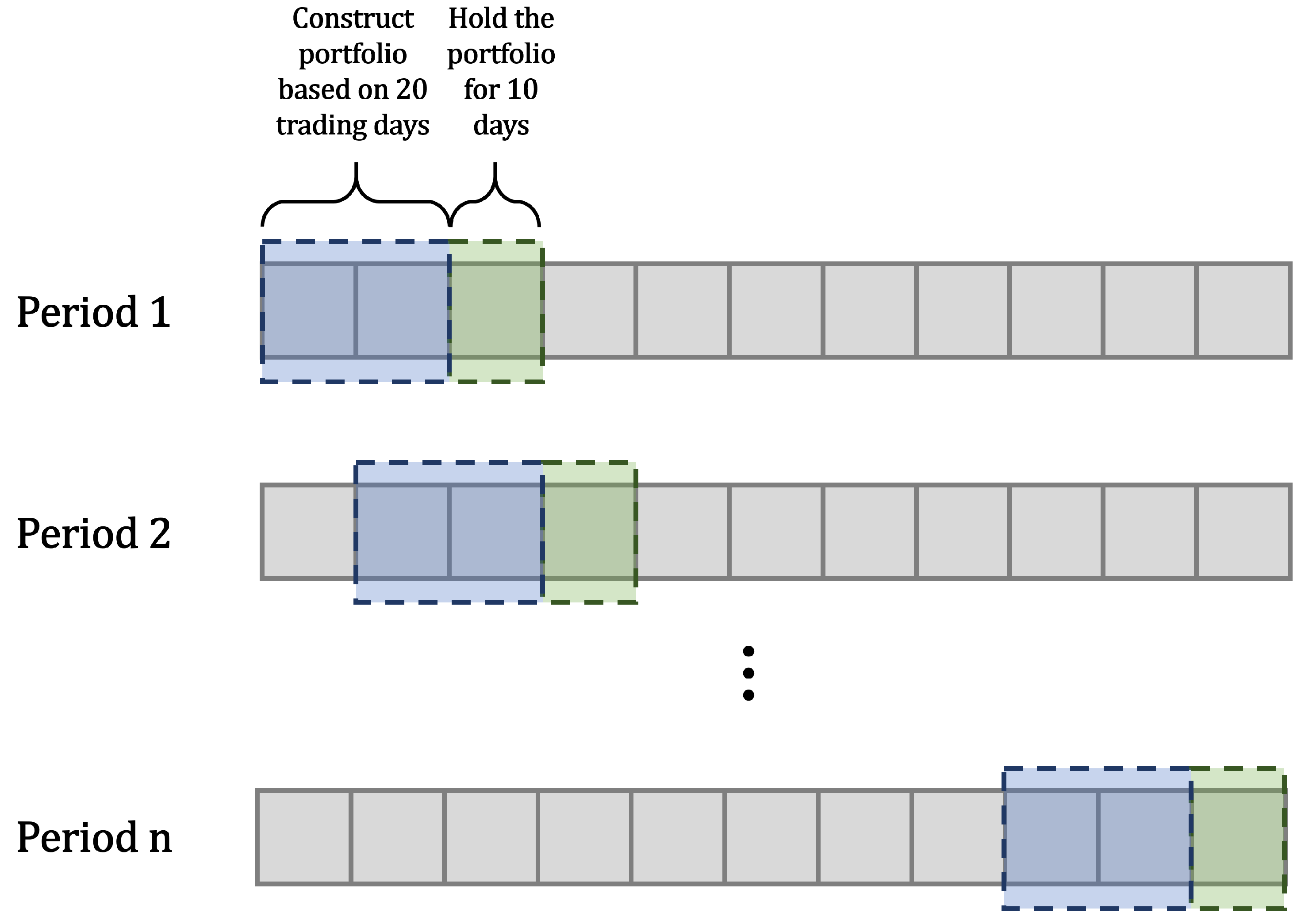
Backtesting: We first extract the high-level features of a candlestick chart of 20 days. The K-means algorithm is then applied to obtain stock market segmentation. We select the asset with the largest Sharpe ratio in each cluster to form a portfolio. This portfolio will be held for one period, which is defined as 10 days in our experiment. After 10 days, we sell this portfolio and obtain the return of this period. The whole process is shown in Figure 3. The total return of the 10 days is the sum of the every stock return in the portfolio.
Asset Allocation: Each stock in the portfolio obtained through our model is allocated of the total investment.
4. Experiments
In this section, we first introduce the dataset and parameters used in the experiment. Then results of two experiments are presented. In the first experiment, we compared the performance of AlexNet [26], VGG [27], DenseNet [28], ResNet [29] and ShuffleNet [30] as encoders in backtesting. In the second experiment, portfolios of different stock numbers are compared. In the third experiment, the investment strategy given by our model is compared with existing funds.
4.1. Dataset and Setting
Our dataset is based on the 1253 representative stocks in the Shanghai Stock Exchange. The stock trading days are from 1 January 2017 to 31 December 2018. The price of the stocks was split-adjusted. For each 20 trading days, a candlestick chart was generated from the four-channel (the lowest, highest, opening, and closing prices) time series of a stock. In total, our dataset contains 600 k candlestick charts generated from 1253 stocks of shanghai stock market. Except for the stock data, we also obtained all funds’ data from Tushare. We used the funds data to compare them with our model’s return.
Our model was trained on a Nvidia 2080TI GPU with 11 GB RAM. The deep learning framework Pytorch and machine learning library Sklearn were used to train our model. The size of the candlestick charts were fixed to during training and evaluating process. The training batch size was 64 and the learning rate is set to . We used the Adam optimizer.
4.2. Experiment 1: Different Network Performance
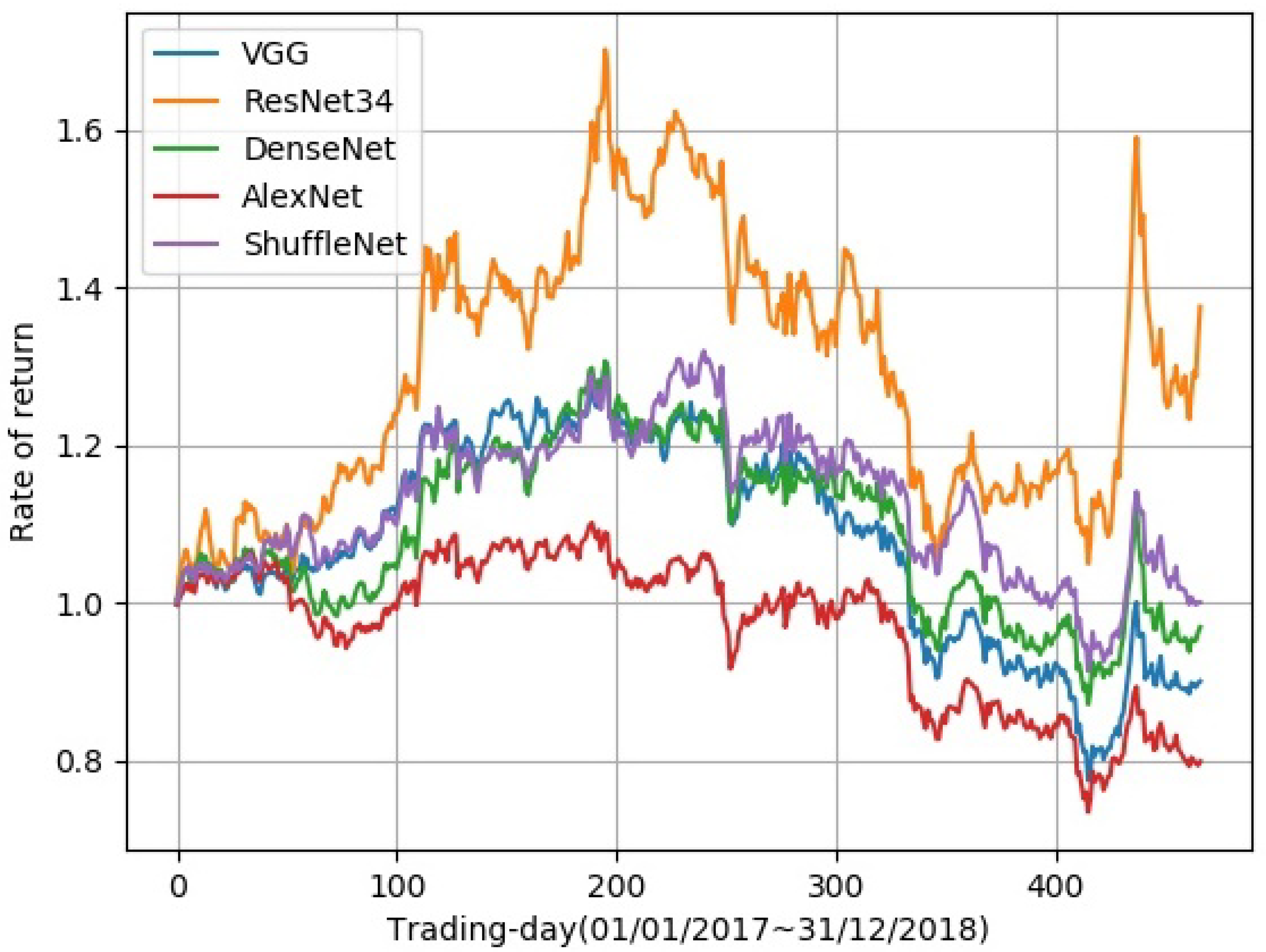
In Figure 2, we show the autoencoder used in our model. Various network architectures were compared to find the best encoder structure, while the decoder structure remained the same, which consists of four upsampling layers. In backtesting, total return, daily Sharpe ratio, max drawdown, daily mean return, monthly mean return, and yearly mean return were used to evaluate the performance of different encoders. For network architectures, we tried AlexNet, VGG, DenseNet, ResNet, and ShuffleNet. As can be seen in Figure 4, ResNet achieved the best result in total return. Additionally, the training speed of ResNet was fast. In Table 1, experimental results are shown. Except for the total return, ResNet also achieved the best results in daily Sharpe ratio, daily mean return, monthly mean return, and yearly mean return.
The experimental results show that ResNet achieved the best results in most indicators and thus has the best overall performance. Thus, we choose ResNet as the network structure of the model encoder in the remaining experiments.
4.3. Experiment 2: Different Stock Numbers of the Portfolio
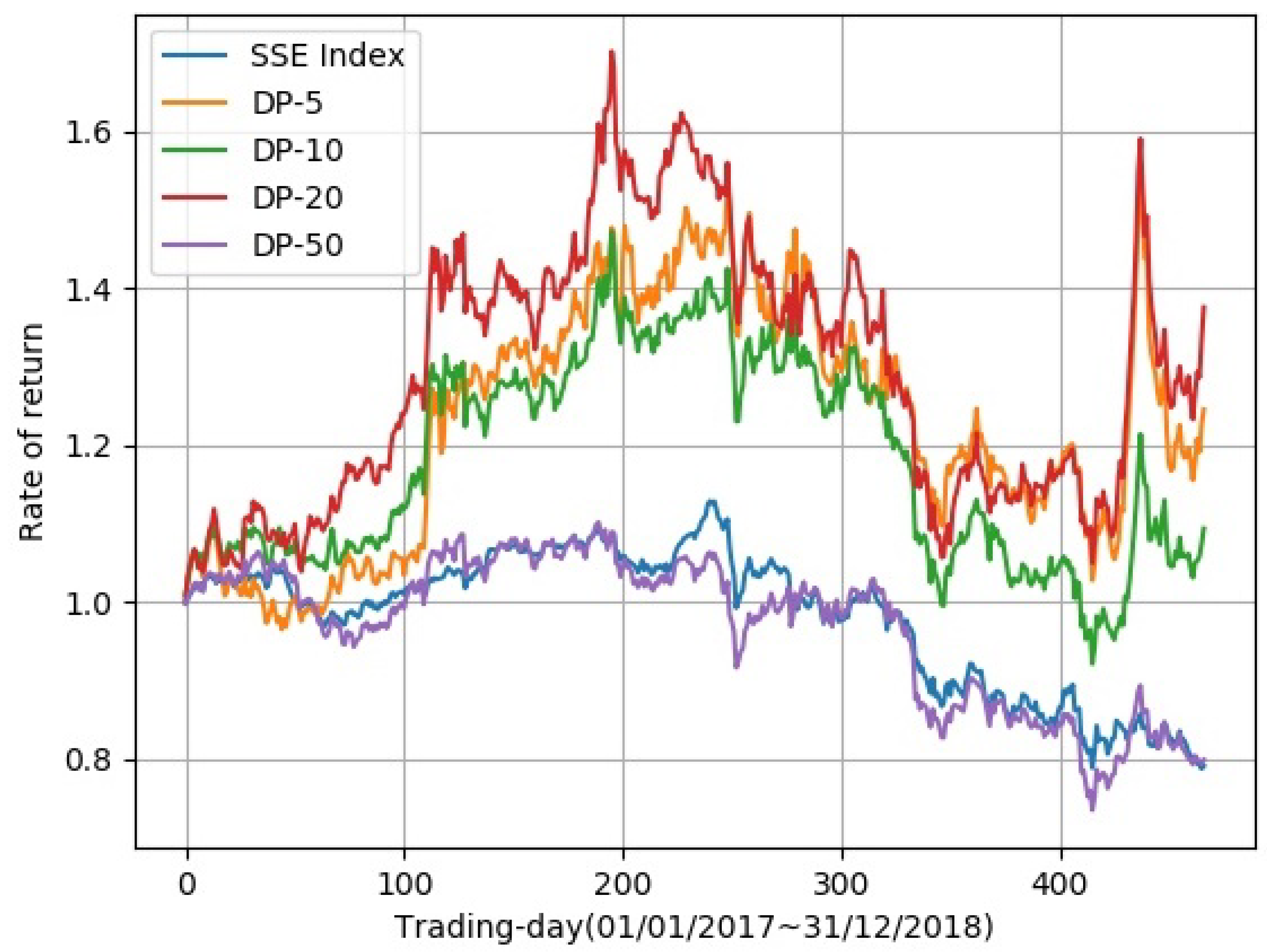
We compared the asset volatility curve of a portfolio of different stock numbers. In Figure 5, asset volatilities of the stock numbers 5, 10, 20, and 50 are displayed. These deep portfolios (DPs) will be named DP-5, DP-10, DP-20, and DP-50, respectively, in the following contents. The abscissa stands for the trading days, and the ordinate is the rate of return. Among all the portfolios, DP-5, DP-10, and DP-20 shared similar trends, while DP-50 had almost the same trend as the SSE Index. This means that DP-50 has no obvious advantages over the SSE Index, and we will pay more attention to portfolios with stock numbers of 5, 10, and 20. In Figure 5, it can be observed that DP-20 achieved the highest rate of return in most trading days. Table 2 shows more detailed data of the proposed deep portfolios. Of all the portfolios, DP-20 achieved the best results in total return, daily Sharpe ratio, daily mean return, monthly mean return, and yearly mean return; however, the max drawdown of DP-20 was the worst. DP-5 obtained the best max drawdown.
It is important to state that an appropriate number of portfolio stocks gives a high total return. Too large a quantity will cause the entire investment portfolio to be highly consistent with the SSE Index. Too small a quantity will make the strategy lack stability. In order to better analyze the performance of our strategy, the SSE Index was compared with our portfolios. Similar to experiment 1, the daily Sharpe ratio, daily mean return, monthly mean return, and yearly mean return were used to evaluate the different portfolios.
4.4. Experiment 3: Comparison with Existing Funds and SSE Index
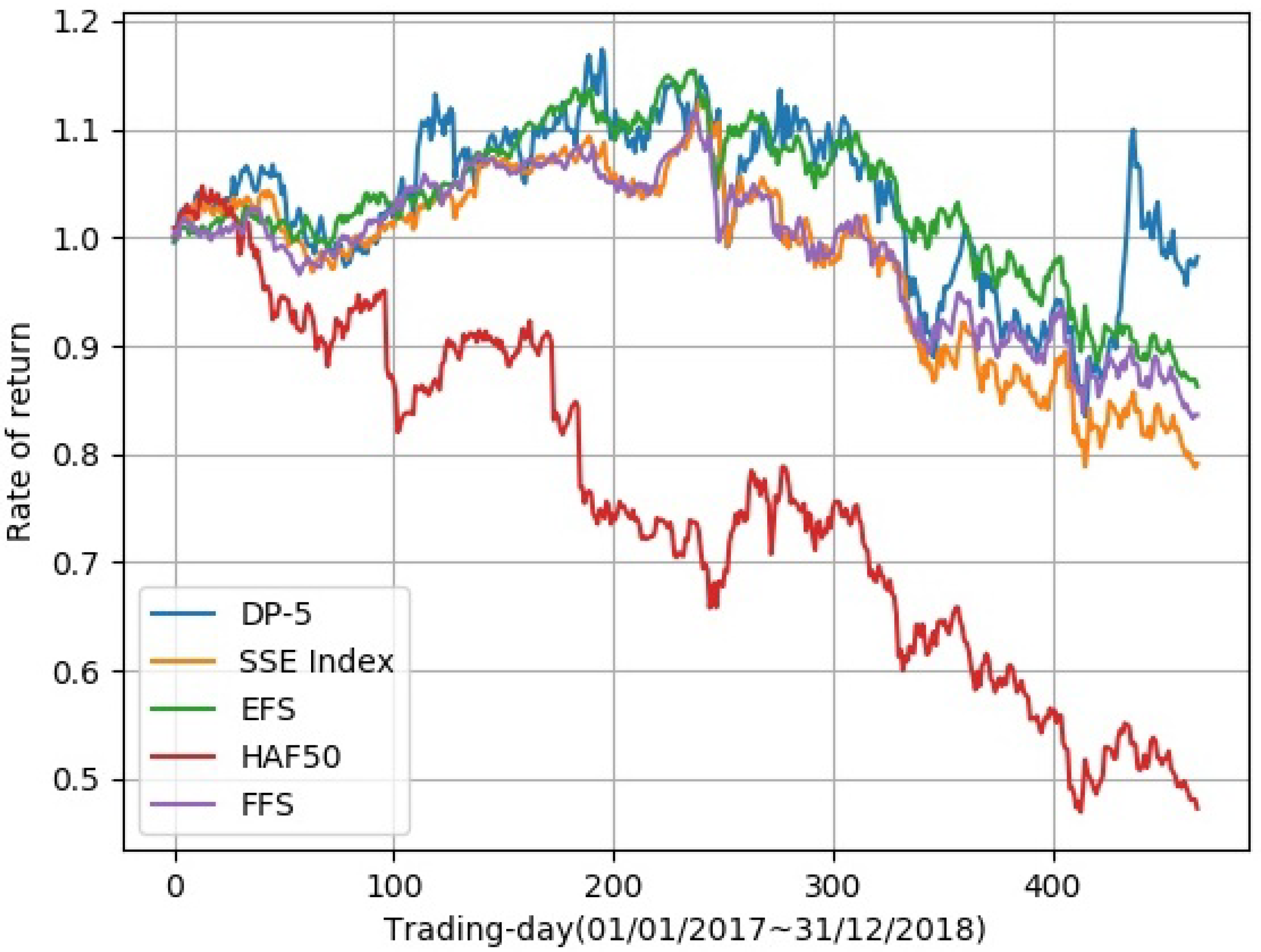
In order to better analyze the effectiveness of our strategy, we compared DP-5 with the E Fund strategy growth (EFS), HuaAn Fund Second-board Market 50 (HAF50), the Fullgoal Fund Shanghai Securities Composite Index (FFS), and the SSE Index.
Figure 6 shows that DP-5 and EFS performed better than the other two funds in rate of returns. As is shown in Table 3, DP-5 obtained the best performance on the total return, daily Sharpe ratio, daily mean return, monthly mean return and yearly mean return. Only on the max drawdown metric did EFS outperform DP-5.
The total return metric showed than our model obtained the biggest total return by a large margin, which means our portfolio will bring more returns in practical investment. Since the Sharpe ratio of DP-5 was bigger than that of other funds and the SSE Index, our portfolio involves a smaller risks at the same return. Max drawdown is an important metric in the finance area. Although we did not obtain the best result in the max drawdown criteria, there was only a small gap between our model and the leading fund, EFS.
Our portfolio also outperformed competitors in three other indicators: daily mean return, monthly mean return, and yearly mean return. It achieved good results in several important indicators, which shows that our model is effective.
We must emphasize that each of the stocks we selected has one of the largest Sharpe ratios from its own cluster. Meanwhile, since the stocks were chosen from different clusters, they have low correlations with each other. As a result, our portfolio yields not only a more attractive risk-adjusted return but also stronger capability against unsystematic risk. Unlike raw data, which give equal attention to different variables, a candlestick chart allocates distinct colors and shapes to different stock trends, thus offering a clearer orientation. Our model can have a better understanding of the market based on the high-level information extracted from candlestick charts, and numerical experiments have already confirmed this viewpoint forcefully.
Portfolio theory points out that non-system risk can be reduced by selecting a group of stocks with a low correlation coefficient. Indicators such as market value and liquidity have been widely used as a similarity measurement by various fund companies in the securities market. In Section 4.4, we compare our model with several companies’ funds. From the results of experiment 3, we can see that our portfolio led on a number of indicators. This proves that the similarity measurement based on the deep features of candlestick charts is effective, and CNN can capture the correlation of stocks.
5. Conclusions
In this paper, we produced a candlestick chart dataset for the Chinese Shanghai Stock Exchange market and proposed a candlestick-based portfolio learning model. This model makes a portfolio through three steps. In the first step, the method learns deep features from candlestick charts using a CAE encoder. In the second step, the K-means algorithm is used to cluster candlestick charts’ features. In the third step, our model builds a portfolio by selecting the stock with the maximal Sharpe ratio in each cluster. Experimental results show that: (1) ResNet has a better effect feature extraction than other networks. (2) Among all portfolios, DP-20 obtained the best performance. (3) Our portfolio exceeds the SSE Index and many well-known funds in many metrics.
For future studies, there is still much room for exploration and improvement of the model. For example, we can also try training the model on longer or shorter time periods (weekly candlestick charts or minute candlestick charts). We can also verify the model in more markets, such as the Shenzhen Stock Exchange market. We can also try to apply more knowledge in the field of deep learning to the quantitative trading.
Author Contributions
Data curation, W.P.; Methodology, W.P.; Resources, X.L.; Writing—original draft, W.P. and J.L.; Writing—review and editing, X.L. All authors have read and agreed to the published version of the manuscript.
Funding
This research received no external funding.
Conflicts of Interest
The authors declare no conflict of interest.
References
- Chan, E. Quantitative Trading: How to Build Your Own Algorithmic Trading Business; John Wiley & Sons: Hoboken, NJ, USA, 2009; Volume 430. [Google Scholar]
- Ritter, J.R. Behavioral finance. Pac. Basin Financ. J. 2003, 11, 429–437. [Google Scholar] [CrossRef]
- Sharpe, W.F. The sharpe ratio. J. Portf. Manag. 1994, 21, 49–58. [Google Scholar] [CrossRef]
- Markowitz, H. Portfolio selection. J. Financ. 1952, 7, 77–91. [Google Scholar]
- Masci, J.; Meier, U.; Cireşan, D.; Schmidhuber, J. Stacked convolutional auto-encoders for hierarchical feature extraction. In Proceedings of the International Conference on Artificial Neural Networks, Espoo, Finland, 14–17 June 2011; pp. 52–59. [Google Scholar]
- Donahue, J.; Krähenbühl, P.; Darrell, T. Adversarial feature learning. arXiv 2016, arXiv:1605.09782. [Google Scholar]
- Amodei, D.; Ananthanarayanan, S.; Anubhai, R.; Bai, J.; Battenberg, E.; Case, C.; Casper, J.; Catanzaro, B.; Cheng, Q.; Chen, G.; et al. Deep speech 2: End-to-end speech recognition in english and mandarin. In Proceedings of the International Conference on Machine Learning, New York, NY, USA, 19–24 June 2016; pp. 173–182. [Google Scholar]
- Mnih, V.; Kavukcuoglu, K.; Silver, D.; Rusu, A.A.; Veness, J.; Bellemare, M.G.; Graves, A.; Riedmiller, M.; Fidjeland, A.K.; Ostrovski, G.; et al. Human-level control through deep reinforcement learning. Nature 2015, 518, 529. [Google Scholar] [CrossRef] [PubMed]
- Fischer, T.; Krauss, C. Deep learning with long short-term memory networks for financial market predictions. Eur. J. Oper. Res. 2018, 270, 654–669. [Google Scholar] [CrossRef] [Green Version]
- Jegadeesh, N.; Titman, S. Returns to buying winners and selling losers: Implications for stock market efficiency. J. Financ. 1993, 48, 65–91. [Google Scholar] [CrossRef]
- Ding, X.; Zhang, Y.; Liu, T.; Duan, J. Deep learning for event-driven stock prediction. In Proceedings of the Twenty-Fourth International Joint Conference on Artificial Intelligence, Buenos Aires, Argentina, 25–31 July 2015. [Google Scholar]
- Akita, R.; Yoshihara, A.; Matsubara, T.; Uehara, K. Deep learning for stock prediction using numerical and textual information. In Proceedings of the 2016 IEEE/ACIS 15th International Conference on Computer and Information Science (ICIS), Okayama, Japan, 26–29 June 2016; pp. 1–6. [Google Scholar]
- Loreggia, A.; Malitsky, Y.; Samulowitz, H.; Saraswat, V. Deep learning for algorithm portfolios. In Proceedings of the Thirtieth AAAI Conference on Artificial Intelligence, Phoenix, AZ, USA, 12–17 February 2016. [Google Scholar]
- El-Yaniv, R. Competitive solutions for online financial problems. ACM Comput. Surv. (CSUR) 1998, 30, 28–69. [Google Scholar] [CrossRef]
- Borodin, A.; El-Yaniv, R.; Gogan, V. On the competitive theory and practice of portfolio selection. In Latin American Symposium on Theoretical Informatics; Springer: Berlin/Heidelberg, Germany, 2000; pp. 173–196. [Google Scholar]
- Pendharkar, P.C.; Cusatis, P. Trading financial indices with reinforcement learning agents. Expert Syst. Appl. 2018, 103, 1–13. [Google Scholar] [CrossRef]
- Wang, J.; Zhang, Y.; Tang, K.; Wu, J.; Xiong, Z. Alphastock: A buying-winners-and-selling-losers investment strategy using interpretable deep reinforcement attention networks. In Proceedings of the 25th ACM SIGKDD International Conference on Knowledge Discovery & Data Mining, Anchorage, AK, USA, 4–8 August 2019; pp. 1900–1908. [Google Scholar]
- Matsubara, T.; Akita, R.; Uehara, K. Stock price prediction by deep neural generative model of news articles. IEICE Trans. Inf. Syst. 2018, 101, 901–908. [Google Scholar] [CrossRef] [Green Version]
- Lim, B.; Zohren, S.; Roberts, S. Enhancing time-series momentum strategies using deep neural networks. J. Financ. Data Sci. 2019, 1, 19–38. [Google Scholar] [CrossRef]
- Nevmyvaka, Y.; Feng, Y.; Kearns, M. Reinforcement learning for optimized trade execution. In Proceedings of the 23rd International Conference on Machine Learning, Pittsburgh, PA, USA, 25–29 June 2006; pp. 673–680. [Google Scholar]
- Vargas, M.R.; De Lima, B.S.; Evsukoff, A.G. Deep learning for stock market prediction from financial news articles. In Proceedings of the 2017 IEEE International Conference on Computational Intelligence and Virtual Environments for Measurement Systems and Applications (CIVEMSA), Annecy, France, 26–28 June 2017; pp. 60–65. [Google Scholar]
- Huang, Y.; Capretz, L.F.; Ho, D. Neural Network Models for Stock Selection Based on Fundamental Analysis. In Proceedings of the 2019 IEEE Canadian Conference of Electrical and Computer Engineering (CCECE), Edmonton, AB, Canada, 5–8 May 2019; pp. 1–4. [Google Scholar]
- Singh, R.; Srivastava, S. Stock prediction using deep learning. Multimed. Tools Appl. 2017, 76, 18569–18584. [Google Scholar] [CrossRef]
- Chong, E.; Han, C.; Park, F.C. Deep learning networks for stock market analysis and prediction: Methodology, data representations, and case studies. Expert Syst. Appl. 2017, 83, 187–205. [Google Scholar] [CrossRef] [Green Version]
- MacQueen, J. Some methods for classification and analysis of multivariate observations. In Proceedings of the Fifth Berkeley Symposium on Mathematical Statistics and Probability, Oakland, CA, USA, 1 January 1967; Volume 1, pp. 281–297. [Google Scholar]
- Krizhevsky, A.; Sutskever, I.; Hinton, G.E. Imagenet classification with deep convolutional neural networks. In Proceedings of the Advances in Neural Information Processing Systems, Lake Tahoe, NV, USA, 3–6 December 2012; pp. 1097–1105. [Google Scholar]
- Simonyan, K.; Zisserman, A. Very deep convolutional networks for large-scale image recognition. arXiv 2014, arXiv:1409.1556. [Google Scholar]
- Huang, G.; Liu, Z.; Van Der Maaten, L.; Weinberger, K.Q. Densely connected convolutional networks. In Proceedings of the IEEE Conference on Computer Vision and Pattern Recognition, Honolulu, HI, USA, 21–26 July 2017; pp. 4700–4708. [Google Scholar]
- He, K.; Zhang, X.; Ren, S.; Sun, J. Deep residual learning for image recognition. In Proceedings of the IEEE Conference on Computer Vision and Pattern Recognition, Las Vegas, NV, USA, 27–30 June 2016; pp. 770–778. [Google Scholar]
- Zhang, X.; Zhou, X.; Lin, M.; Sun, J. Shufflenet: An extremely efficient convolutional neural network for mobile devices. In Proceedings of the IEEE Conference on Computer Vision and Pattern Recognition, Salt Lake City, UT, USA, 18–23 June 2018; pp. 6848–6856. [Google Scholar]
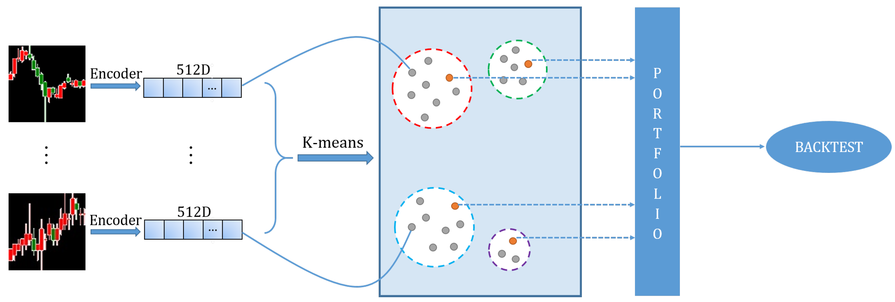
Figure 1.
Schematic illustration of our investment decision pipeline.

Figure 2.
The structure of the CAE. The encoder structure is ResNet-34. The decoder has four upsampling layers.
Figure 2.
The structure of the CAE. The encoder structure is ResNet-34. The decoder has four upsampling layers.

Figure 3.
The process of backtesting. For each period, we obtain the portfolio based on 20 trading days and hold it for 10 days. This repeats for all periods. n is the number of total trading periods.
Figure 3.
The process of backtesting. For each period, we obtain the portfolio based on 20 trading days and hold it for 10 days. This repeats for all periods. n is the number of total trading periods.

Figure 4.
Comparison of different networks’ performance in total return. ResNet obtained the best result among all network structures. The abscissa is the time, ranging from the first trading day on 1 January 2017 to the last trading day on 31 December 2018. The ordinate is the rate of return.
Figure 4.
Comparison of different networks’ performance in total return. ResNet obtained the best result among all network structures. The abscissa is the time, ranging from the first trading day on 1 January 2017 to the last trading day on 31 December 2018. The ordinate is the rate of return.

Figure 5.
Comparison between different numbers of clusters in portfolios. The abscissa is the time from the first trading day on 1 January 2017 to the last trading day on 31 December 2018. The ordinate is the rate of return.
Figure 5.
Comparison between different numbers of clusters in portfolios. The abscissa is the time from the first trading day on 1 January 2017 to the last trading day on 31 December 2018. The ordinate is the rate of return.

Figure 6.
Comparison with existing funds and the SSE Index. The abscissa is the time from the first trading day on 1 January 2017 to the last trading day on 31 December 2018. The ordinate is the rate of return.
Figure 6.
Comparison with existing funds and the SSE Index. The abscissa is the time from the first trading day on 1 January 2017 to the last trading day on 31 December 2018. The ordinate is the rate of return.


Table 1.
Different networks’ performance.
| VGG | DeseNet | ResNet | AlexNet | ShuffleNet | |
|---|---|---|---|---|---|
| Total Ret. | |||||
| Daily Sharpe | |||||
| Max Drawdown | |||||
| Daily Mean Ret. | |||||
| Monthly Mean Ret. | |||||
| Yearly Mean Ret. |
Table 2.
Comparison of clustering numbers.
| DP-5 | DP-10 | DP-20 | DP-50 | SSE Index | |
|---|---|---|---|---|---|
| Total Ret. | |||||
| Daily Sharpe | |||||
| Max Drawdown | |||||
| Daily Mean Ret. | |||||
| Monthly Mean Ret. | |||||
| Yearly Mean Ret. |
Table 3.
Comparison of well-known funds.
| DP-5 | EFS | HAF | FFS | SSE Index | |
|---|---|---|---|---|---|
| Total Ret. | |||||
| Daily Sharpe | |||||
| Max Drawdown | |||||
| Daily Mean Ret. | |||||
| Monthly Mean Ret. | |||||
| Yearly Mean Ret. |
Publisher’s Note: MDPI stays neutral with regard to jurisdictional claims in published maps and institutional affiliations. |
© 2020 by the authors. Licensee MDPI, Basel, Switzerland. This article is an open access article distributed under the terms and conditions of the Creative Commons Attribution (CC BY) license (http://creativecommons.org/licenses/by/4.0/).
Share and Cite
MDPI and ACS Style
Pan, W.; Li, J.; Li, X. Portfolio Learning Based on Deep Learning. Future Internet 2020, 12, 202. https://0-doi-org.brum.beds.ac.uk/10.3390/fi12110202
AMA Style
Pan W, Li J, Li X. Portfolio Learning Based on Deep Learning. Future Internet. 2020; 12(11):202. https://0-doi-org.brum.beds.ac.uk/10.3390/fi12110202
Chicago/Turabian StylePan, Wei, Jide Li, and Xiaoqiang Li. 2020. "Portfolio Learning Based on Deep Learning" Future Internet 12, no. 11: 202. https://0-doi-org.brum.beds.ac.uk/10.3390/fi12110202
Note that from the first issue of 2016, this journal uses article numbers instead of page numbers. See further details here.