Comparing Modeled Emissions from Wildfire and Prescribed Burning of Post-Thinning Fuel: A Case Study of the 2016 Pioneer Fire

Department of Forest, Rangeland, and Fire Sciences, College of Natural Resources, University of Idaho, Moscow, ID 83844, USA
*
Author to whom correspondence should be addressed.
Fire 2019, 2(2), 22; https://0-doi-org.brum.beds.ac.uk/10.3390/fire2020022
Submission received: 6 April 2019
/
Revised: 1 May 2019
/
Accepted: 3 May 2019
/
Published: 9 May 2019
Abstract
:Prescribed fire is often used by land managers as an effective means of implementing fuel treatments to achieve a variety of goals. Smoke generated from these activities can put them at odds with air quality regulations. We set out to characterize the emission tradeoff between wildfire and prescribed fire in activity fuels from thinning in a case study of mixed conifer forest within the Boise National Forest in central Idaho. Custom fuelbeds were developed using information from the forest and emissions were modeled and compared for four scenarios, as follows: Untreated fuels burned in wildfire (UNW), prescribed fire in activity fuels left from thinning (TRX), a wildfire ignited on the post-treatment landscape (PTW), and the combined emissions from TRX followed by PTW (COM). The modeled mean total emissions from TRX were approximately 5% lower, compared to UNW, and between 2–46% lower for individual pollutants. The modeled emissions from PTW were approximately 70% lower than UNW. For the COM scenario, emissions were not significantly different from the UNW scenario for any pollutants, but for CO2. However, for the COM scenario, cumulative emissions would have been comprised of two events occurring at separate times, each with lower emissions than if they occurred at once.
1. Introduction
Land managers steward large tracts of public lands to preserve multiple, and sometimes competing, public values. In the western United States, historical fire suppression [1,2] and a shift to a warmer drier climate [3,4] contribute to a seasonal trend of large and often severe wildfires [5,6]. In this environment, land managers work to meet the requirements of the National Fire Plan [7], the Healthy Forest Restoration Act [8], and goals of the 2014 National Cohesive Strategy [9], which include the restoration and maintenance of natural landscapes and resilience to wildfire. One important tool to achieve these goals and promote forest health is the use of fuel treatments, often a combination of mechanically removing and burning excess biomass, to meet ecological objectives and reduce hazardous fuels that contribute to the spread and severity of wildfires. Such fuel treatment is an important feature of modern adaptive management techniques [10] that support forest health and wildfire hazard reduction.
At the same time, smoke is one of the key concerns when weighing the costs and benefits of fuel treatments employing prescribed fire [11]. Smoke from these fires contains pollutants addressed by the Clean Air Act [12] and has the potential to impact public health [13]. Such consequences must be seriously considered when addressing prescribed fire smoke. As wildfires show no sign of subsiding and smoke continues be an important issue for communities and policy makers, and land managers must weigh the costs and benefits of prescribed fire smoke to those of wildfire smoke. This is particularly important for particulate matter, the pollutant in smoke often of greatest concern from both human health and regulatory standpoints [14]. Particulate matter is reported by the size of the particulates, commonly PM2.5 and PM10, referring to particulates 2.5 and 10 micrometers in size, respectively. The smaller particles are of greater concern to human health. Other constituents that make up a large percentage of smoke emissions, though often of less regulatory and health concern relative to particulate matter, include carbon monoxide, carbon dioxide, methane, nitrogen dioxide, and volatile organic compounds.
A literature review focusing on comparing the quantities of smoke produced in wild and prescribed fires yielded a relatively small body of work compared to other wildland fire topics, such as fuel loading and quantification. Ottmar [15] noted that, generally, two to four times higher fuel consumption and emissions take place in wildfires compared to prescribed fires, mainly via increased fuel consumption under drier hotter conditions and the additional involvement of the tree canopy in the fire. Other work on this topic took place during the 1990s and primarily compared historical and current emission levels [16,17]. Two recent studies compared the emission tradeoff regarding treatments. One study in a western mixed conifer forest found that fuel treatments reduced the impact of downwind smoke effects mainly via a reduction in fire behavior [18]. Another study, which primarily examined salvage logging, reported reductions in PM2.5 production [19].
Our study uses the case example of the 2016 Pioneer Fire on part of the Boise National Forest to model and compare emissions under post-treatment prescribed fire and wildfire scenarios. We simulate emissions from this wildfire under the July 2016 fuel moisture conditions and compare those to the simulated results for a proposed treatment scenario, which had been planned for the area but was not implemented because of the wildfire. We compare emissions from the four following scenarios: (A) The wildfire burning through untreated forest under July 2016 moisture conditions (UNW); (B) pile burn and prescribed fire in fuels left from thinning, burned under prescribed moisture conditions (TRX); (C) wildfire burning under the same July 2016 moisture conditions as UNW, but after the stand would have been thinned and the material burned (PTW); and (D) the combination of scenarios B and C, the total emissions from a treatment followed by wildfire (COM).
2. Materials and Methods
2.1. Project Area and Stands
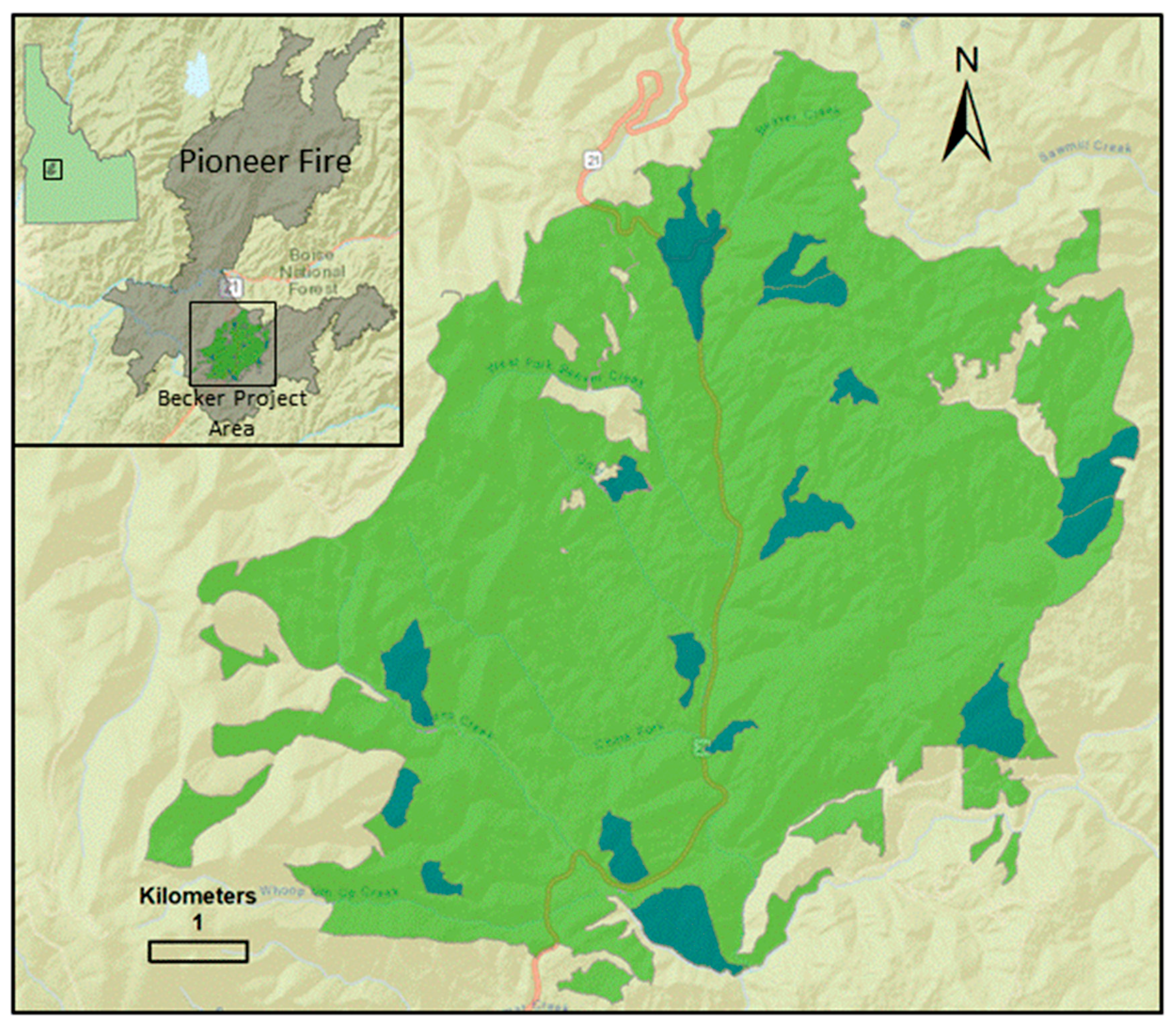
The Pioneer Fire of 2016 was one of the largest and most expensive forest fires to occur in the state of Idaho in recent history, burning approximately 76,081 hectares through July and August. Among the areas within the fire perimeter was the Boise National Forest’s Becker Project Area (Figure 1). The Becker Project Area encompassed 7985 hectares of low to mid elevation forest between 1524–2133 m (Figure 1), with strongly dissected drainage patterns throughout.
Most of the project area occupied the non-lethal or mixed severity fire regimes (Table 1) and consisted of mature ponderosa pine (Pinus ponderosa), Douglas-fir (Pseudotsuga menziesii), and subalpine fir (Abies lasiocarpa), with lodgepole pine (Pinus contorta), which had grown into the older stands over the last several decades of fire exclusion.
2.2. Study Design
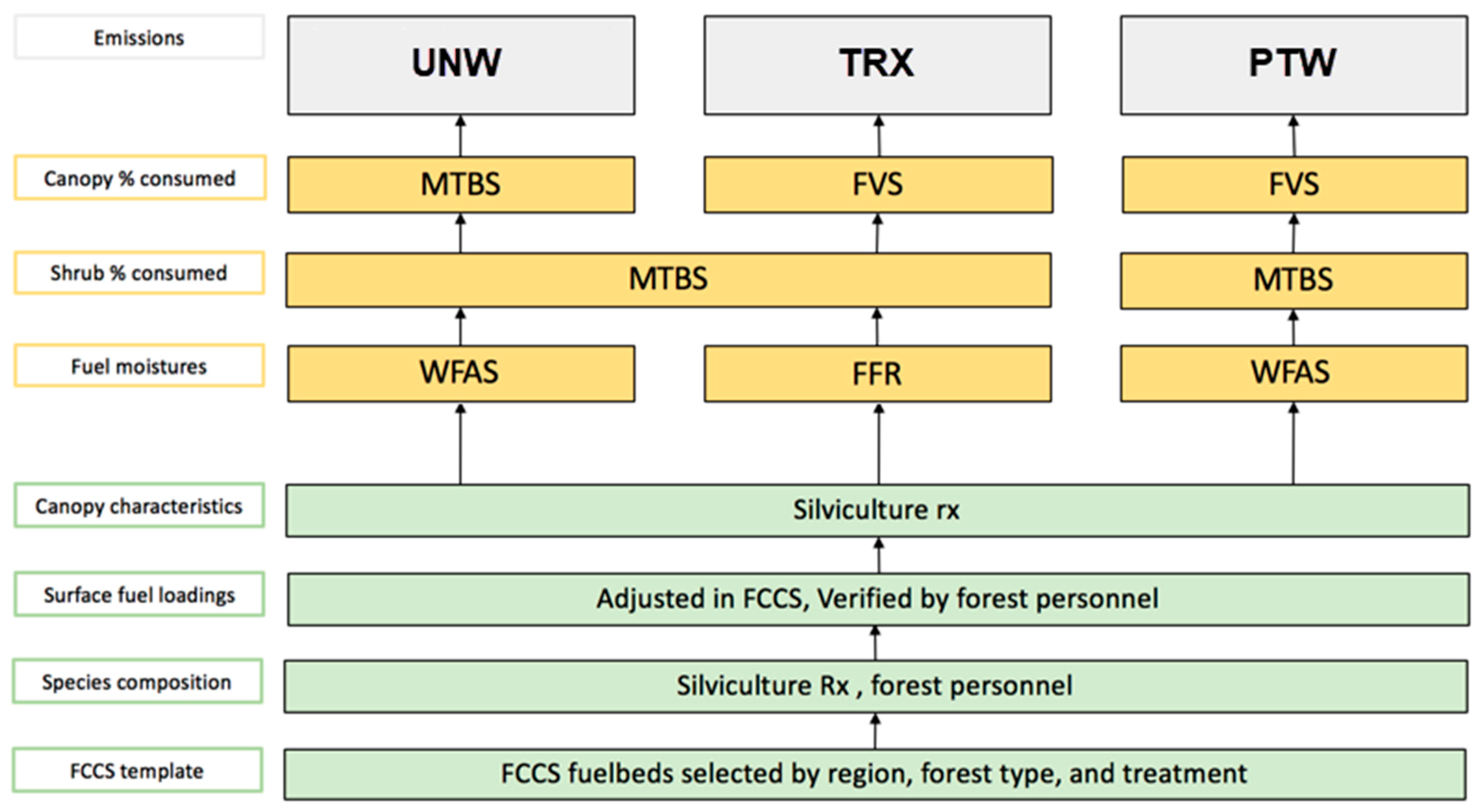
For this study, we contacted forest staff and obtained the silvicultural prescription [22] describing the site conditions and proposed mechanical treatments, a fire and fuels report [23] describing the proposed prescribed fire treatments, forest stand data, and a series of Forest Vegetation Simulator Fire and Fuels Extension (FVS-FFE) model outputs, created in preparation of the two documents, which described the change in canopy characteristics. From this material we gathered a total of 16 representative stands that were described across all information sources. Using the Fuel Characteristic Classification System (FCCS) fuelbeds as a baseline (described later), we applied information from the National Forest to create custom fuelbeds to represent the stands. Canopy consumption, required for emission modeling, was informed by the Monitoring Trends in Burn Severity (MTBS) [24] data from the Pioneer fire for UNW, and forest FVS-FFE [25] outputs for all other scenarios. We assessed the available FVS-FEE outputs of canopy characteristics computed by the forest staff to be a more accurate estimate for use in the TRX and PTW scenarios, compared to adjusting down the MTBS values. FVS-FFE does not address shrubs, so we relied on MTBS for all scenarios when addressing shrubs. Woody fuel moistures for the wildfire scenarios were informed by Wildland Fire Assessment System (WFAS) fuel moistures [26]. Fuel moistures for the prescribed fire scenarios were informed by the prescribed moistures in the Fire and Fuels Report. This approach is represented in Figure 2.
2.3. Proposed Treatments
Treatments proposed for the Becker project consisted of a combination of pre-commercial and commercial thinning, followed by fuel reduction achieved by pile burning and broadcast burning (Table 2). The goals of these treatments included a reduction in tree density, shifting species composition toward larger ponderosa pine and Douglas-fir trees, and reducing the potential for a high severity wildfire with a reduction of surface fuel and canopy density and an increase in canopy base height. To simplify our comparison, we considered the emissions from piles and from broadcast burns together (TRX). However, in practice, piles would be burned first and a crew would return later to ignite the broadcast burn.
2.4. Fuelbed Modeling with Stands and Treatments
To model scenarios UNW, TRX, and PTW we chose to create Fuels Characteristic Classification System (FCCS) fuelbeds. These fuelbeds are the required inputs for the consumption and emissions model used in our next steps. As a starting point, we chose fuelbeds in the Northeast Oregon Fuelbed Pathways Handbook [27]. We selected those fuelbeds because of the relative proximity to southern Idaho, with similar forest species, and a large selection of treated fuelbeds to use as a baseline. The fuel types in Table 3 were chosen by cross-walking tree species, age, slope, aspect, and elevation to FCCS fuelbeds for pretreatment stands, treated stands, and post-treatment stands. Specifically, we selected three forest types, as follows: Warm dry Douglas-fir ponderosa pine and fir, cool moist fir, and cold dry subalpine forest types (Table 3).
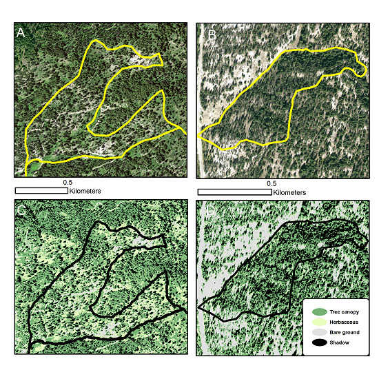
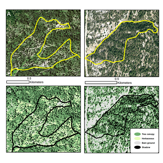
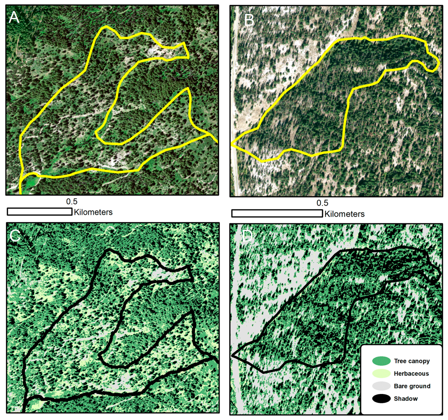
Next, adjustments were made to the species composition and tree density pre- and post-treatment, based on the forest silvicultural prescription [22]. Pre- and post-treatment canopy base heights were adjusted to match those of the FVS-FFE outputs [23]. We applied tree density and canopy base height values to FCCS’s mid and under story in the same proportions they were represented in the default fuelbeds relative to the overstory (i.e., if the FCCS default contained half the tree density in the overstory and half in the mid story, we applied half the tree density from the data in the overstory and half in the mid story). To determine the percent of canopy cover, another FCCS input, we used remote sensing of fine scale imagery to obtain an estimate of the canopy cover within each proposed treatment area prior to the Pioneer fire. One-meter resolution National Agriculture Imagery Program (NAIP) imagery from 2015 was classified into four cover classes, as follows: Tree canopy, herbaceous, bare ground, and shadow, as shown in two example stands in Figure 3. We used a maximum likelihood supervised classification technique in the Image Classification tool in ArcGIS. Canopy cover for the treatment area was calculated by dividing the proportion of tree canopy plus shadow by the sum of tree canopy, herbaceous, and shadow. Bare ground was excluded from the denominator to exclude rocky outcrops and roads from the canopy cover estimate.
FCCS base fuel loadings for fine and coarse woody fuels, duff, and litter, were used for the pre-treatment fuelbeds. The FCCS base fuel loading values for TRX and PTW fuelbeds were adjusted in consultation with the District Fuels Assistant Fire Management Officer [28] to ensure we modeled the UNW, TRX, and PTW woody fuel for that forest as closely as possible (Table 3). Shrub cover by species was also reviewed and adjusted as needed during this consultation. The resulting customized fuelbeds for pre-treatment, post-mechanical treatment, and post prescribed fire treatment are available for download as supplemental material to this article.
2.5. Emissions Modeling and Inputs
Emission modeling was simulated using the Fire Environment Research Application’s Fuel and Fire Tools (FFT) modeling suite [29], version 2.0.1022. This application provides for the creation and customization of FCCS fuelbeds and incorporates the Consume fuel consumption and emissions model (https://www.fs.fed.us/pnw/fera/research/smoke/consume/), with which we produced emissions estimates for each scenario, including those for carbon monoxide and dioxide, particulate matter 2.5 and 10, methane, and non-methane hydrocarbons. We chose this approach because Consume is frequently used to address consumption and emissions in many fire and air quality applications, including the BlueSky modeling framework [30], the Wildland Fire Emissions Information System [31], and the US National Emissions Inventories [32]. In addition to the fuelbeds developed earlier, the model requires fuel moistures and estimates for canopy and shrub consumption.
The TRX woody fuel and duff moistures were taken from the proposed prescription conditions (Table 4) to represent moistures typical in the fall prescribed burning season. UNW and PTW woody fuel moistures were taken from the Forest Service Wildland Fuels Assessment System (WFAS) [26], which reported measured fuel moistures from the Town Creek site between 27 and 31 July 2016 (Table 4). This site location was the closest Remote Automated Weather Station (RAWS) in location and elevation to the burn area and the date range matches the time the wildfire burned through the treatment area, according to the fire progression information as reported by GEOMAC [33]. Measured duff moistures are not included in WFAS, so these values were therefore taken from the Forest Fire and Fuels Report for the wildfire and prescribed fire. Litter moistures for prescribed and wildfire scenarios were derived using the fine woody fuel moistures for various size classes and their inclusion in the litter layer at various depths [34].
To represent canopy and shrub consumption for each stand during the UNW scenario, we used the MTBS fire severity map generated for the 2016 Pioneer fire and assigned a severity class to each stand based on that reported for the majority of pixels within that stand. If severity was missing from the data, high severity was assigned to the stand. Once severity was assigned, the corresponding canopy and shrub consumption was assigned using the FireMon Burn Severity Composite Burn Index long form [35], assigning 90% and 60% canopy kill for high and moderate severity stands, respectively, and 98% shrub kill for all stands. For TRX, canopy kill from the FVS-FFE output [23] was used and shrub kill was set as 20%, a low severity based on FireMon [35]. For the PTW scenario, the FVS-FFE output was used for canopy kill and 70% kill for shrubs, corresponding to moderate severity [35]. The TRX conditions describing days since rain and duration of ignition were verified by forest personnel [28].
2.6. Statistical Analysis
The difference in emissions production for the 16 stands under the four emission scenarios was statistically tested in R Statistical Software, version 3.5.0 [36]. Levene’s test for homogeneity of variance [37] indicated the results met the assumptions required for parametric analysis. Significant differences at the alpha = 0.05 significance level was first tested using one-way analysis of variance [38]. If significant differences were detected, further pairwise testing to identify the specific group differences was conducted using Tukey’s honestly significant difference (HSD) test [39].
3. Results
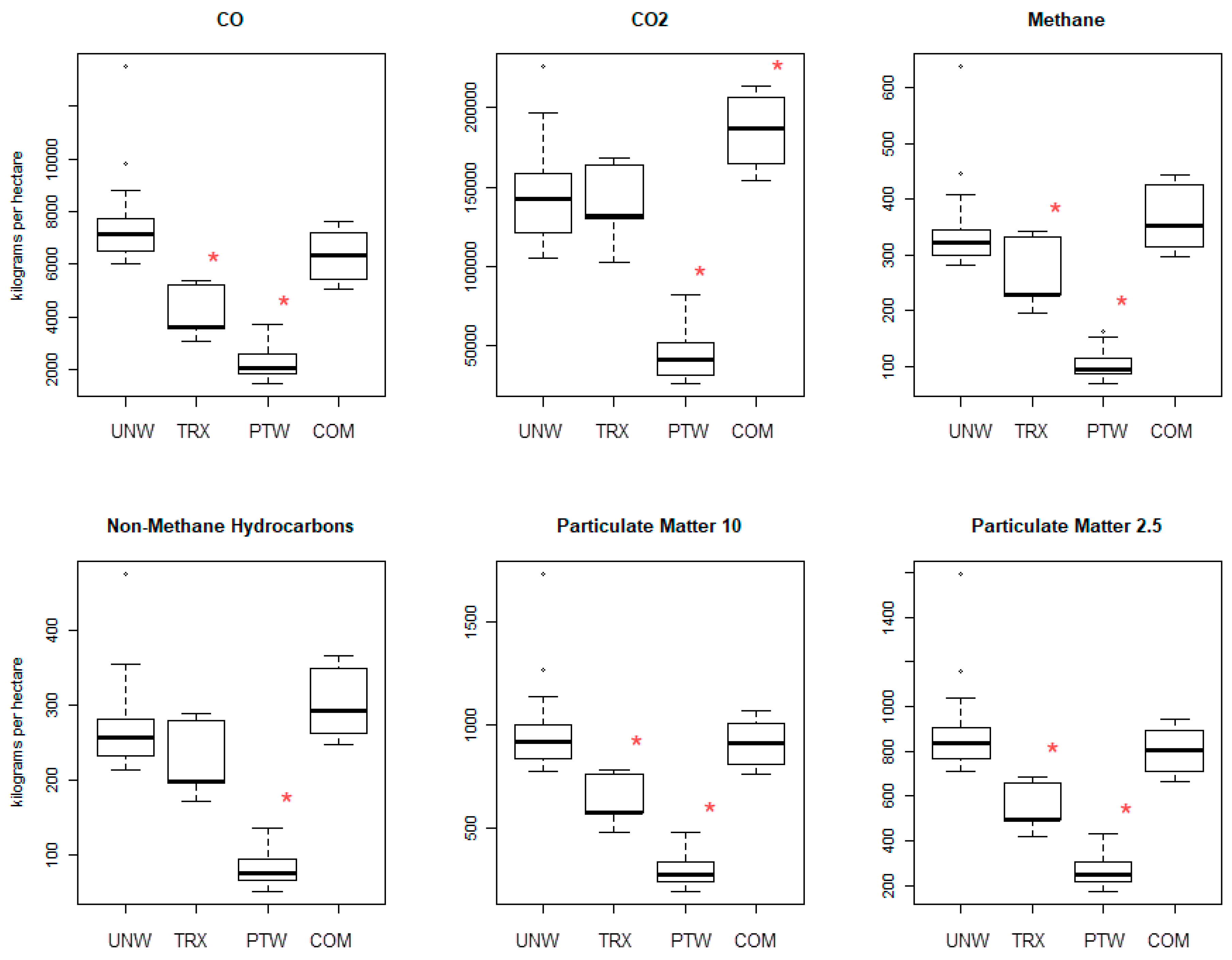
Modeled emissions for each pollutant type (CO, CH4, PM2.5, etc.) from TRX are 2–46% lower than those generated in a wildfire event in untreated stands (UNW), varying by pollutant, except for CO2 and hydrocarbons, for which the percent decrease was not significant. The difference for each pollutant is displayed in Figure 4. For PTW, the modeled emissions are less than a third of the emissions generated by UNW (Table 5, Figure 4), regardless of pollutant type.
Next, we combined emissions from TRX and the wildfire burning through the post-treatment landscape (PTW) to give an overall comparison (COM). CO2 emissions for COM were higher than (UNW), while other pollutants were not found to differ significantly from a statistical perspective. However, it is important to note that the COM scenario is composed of two events, the prescribed fire treatment emissions and a post-treatment wildfire, which would take place at different points in time. Thus, the emissions result from two lower intensity events relative to wildfire in untreated forest stands.
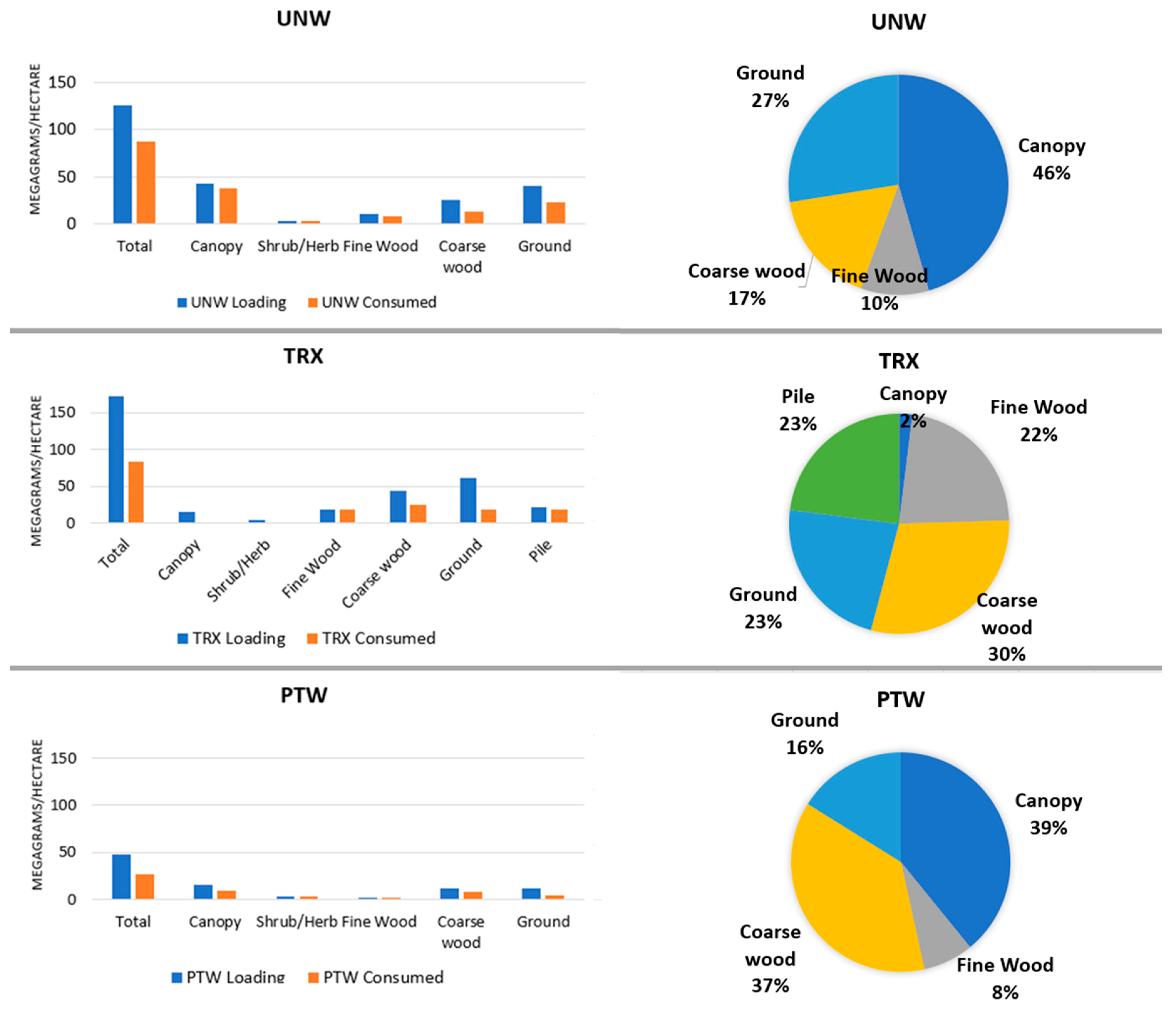
Components of the fuelbed (ground, fine and coarse woody material, pile, and canopy fuels) contributed to different proportions of the emissions, depending upon the fire scenario (Figure 5). For UNW, canopy and ground fuel (duff and litter) produced most of the emissions, followed by coarse and fine woody debris, respectively. When prescribed fire was modeled for the fuel left from-mechanical-thinning (TRX), overall loading was higher, but consumption was lower and most emissions came from coarse woody debris, piles, ground fuel, and fine woody fuel consumption, respectively. This difference is expected given that the mechanical treatments add woody fuel to the forest floor and reduce the fuel loading and density in the canopy. In the PTW scenario, the greatest emissions were produced from the canopy, followed by coarse woody fuel, ground fuel, and fine woody fuel, respectively.
4. Discussion
4.1. Emission Production
The modeled lower emissions in the TRX scenario, compared to the UNW scenario, are due to a combination of lower canopy fuel consumption and running the model under the higher fuel moistures, typical of fall season prescribed fire. Focusing on the fuel aspect, the most obvious difference is the consumption of canopy fuel (Figure 5). Canopy fuel loading was 64% lower and canopy consumption was 96% lower for the TRX, compared to UNW. The lower canopy fuel loading was due to the reduced tree density and increased canopy base heights [22,23]. In addition to lower available fuel loading there was also significantly lower canopy consumption in the post-treatment (PTW) scenario. FFT does not calculate percent of the canopy burned. Rather, the user provides the model with that information. In our case, we used the MTBS fire severity geospatial layer to assign a wildfire severity for each stand and correlate the percent of canopy consumption to that stand. This correlation was performed by cross-walking severity to canopy mortality, according to Key and Benson [35]. Since many of the stands were mapped under high fire severity, a higher percent consumption was assigned in the UNW scenario.
A higher ground fuel consumption in UNW also contributed to the higher emissions, relative to that of the post-treatment stands (TRX). This is important not only due to the change in quantity of fuel consumed, but also combustion efficiency. Combustion of fuels prone to smoldering, such as duff and coarse woody debris, is associated with higher emission factors [40,41]. The higher combustion efficiency of flaming combustion, such as that typical of burning piles, often produces lower particulate emissions but a higher CO2:CO ratio [14]. We suspect this is the reason for the higher CO2 emission released in the COM modeling scenario. The post-treatment fuelbeds indicated a mean consumption reduction of 4%, relative to the wildfire scenario, even though the loading of these fuels was 36% higher due to treatment activity. These differences are likely due to the higher percent fuel moisture in the post-treatment prescribed burn scenario, 125 and 13 percent fuel moisture for duff and litter, respectively, compared to 35 and 4 percent fuel moisture under a wildfire scenario.
It is important to note the relatively high woody fuel loading in our TRX scenario (fuels resulting from mechanical thinning activities). These fuel loads exceed those of other mixed conifer stands where thinning activity fuel is not present [42,43,44] and matches those of post logging fuels [45]. The high woody fuel loading is due to the combination of material that would have been left on the ground from treatment activities, as well as the wood piles that would also be present. For simplicity, we reported the burning of these under the one TRX scenario, however in practice the forest would burn the piles at one point in time and return to conduct a broadcast burn to remove the rest of the fuels later. During the time these fuels are left on site, before they could be burned, they would increase the overall fire hazard [23]. If such fuels had not been removed, either by controlled burning or removal from the site, they would have the potential to continue to increase the fire and smoke hazard. The increase in hazard when activity fuels are left on site has been recognized in research by Bernau et al. [46]. PTW shows a similar pattern in consumption to that of UNW. However the overall fuel loading is greatly reduced in the PTW fuelbeds, thus there is far less fuel to consume. It is important to note that fire exclusion had allowed for several decades of fuel accumulation in our study area.
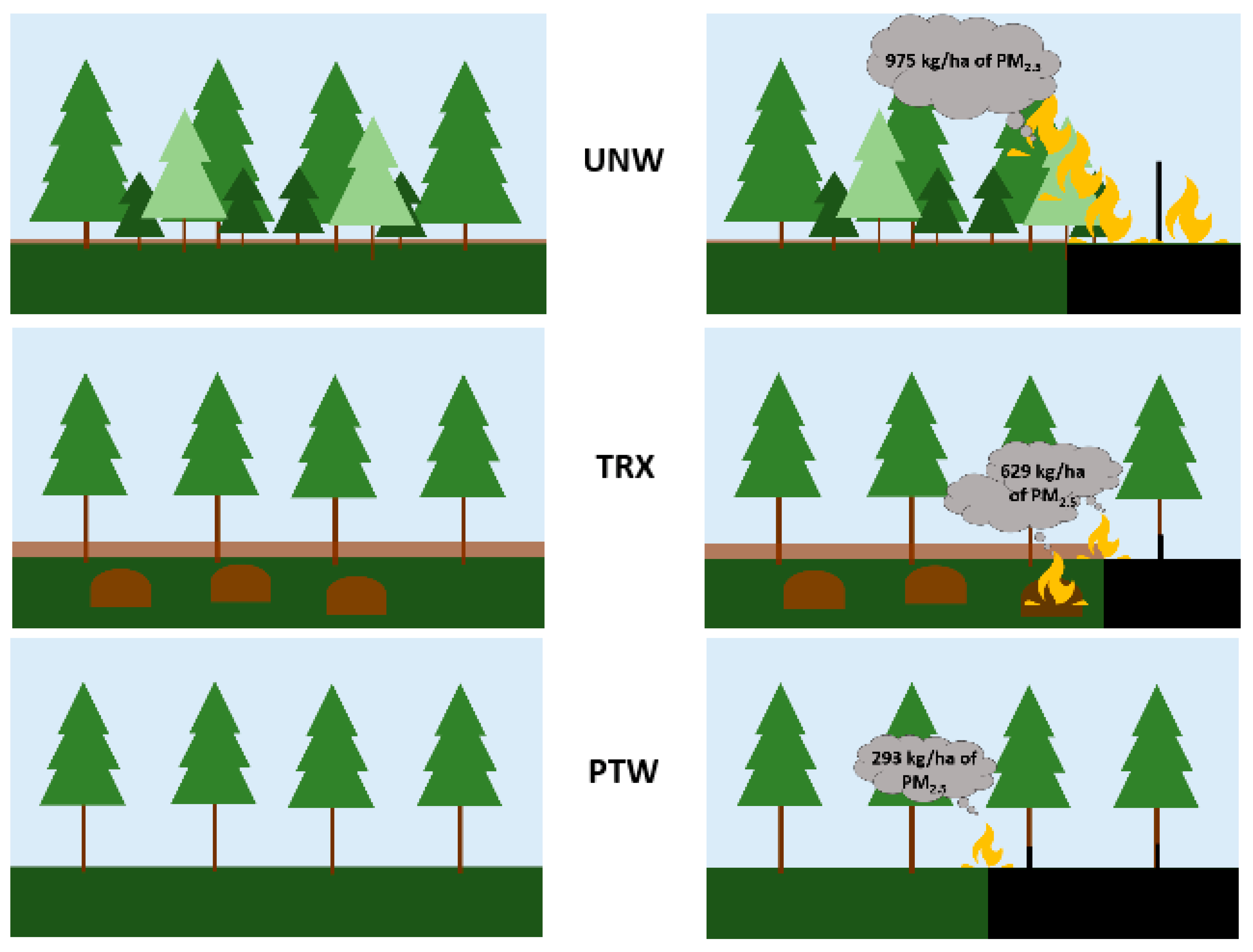
We found total mean emissions from the TRX scenario to be approximately 5% lower than modeled UNW emissions. This difference is less than that reported by Huff [17] or Ottmar [15]. Huff’s work, however, only evaluated PM10 and Ottmar focused on fuelbeds with similar fuel loading, where burn conditions (wild and prescribed) varied, considering the influence of fuel moisture and canopy fuels, but not the addition of activity fuels generated in thinning treatments, as is the case in our scenario. This is a different approach than our study, which evaluated emissions from untreated fuel loading under wildfire conditions, emissions in stands where the surface fuel loading was increased because of thinning and burned under prescribed conditions, and finally emissions from a wildfire in the new post-thinned and post prescribed burn landscape. The impact of treatments (TRX) represented for our study can be summarized as a shift of fuel from the overstory to the surface as stands are thinned, followed by the removal of that fuel by burning, to achieve a more resilient stand in the event that future wildfires occur (Figure 6).
The overall reduction in emissions following a treatment is broadly in agreement with results from Stevens et al. [18], who modeled emissions from treatments using Consume in Sierra Nevada’s mixed conifer forest, as well as Johnson et al. [19], who evaluated salvage logging and pile burning. Our study supports the findings of previous research, while providing a detailed example of southern Idaho mixed conifer emissions, when fuel from mechanical thinning is left and burned under prescribed conditions, and emissions generated in the event of a post-treatment wildfire. There is a need for future studies that account for both differences in fuel and smoke dispersion mechanisms to inform the comparison between wildfire and prescribed fire emissions.
Another key aspect of emission production is the emission factors employed by a model. In addition to fuel loading, consumption, and moisture, emission factors also contribute to differences in emission characteristics between scenarios. Of the emissions modeled herein, CO2 makes up the greatest percentage of the emissions, exceeding the mass of fuel consumed. The CO2 emission factor has remained similar in past versions of Consume and represents such a large proportion of overall emissions due to the nature of wood combustion. If this study were repeated with future planned versions of emissions modeling software, we would expect the relative relationship between treatments and emissions quantities to be similar. However, the quantity of emissions, specifically particulate matter, may likely be different. Recent emission factor research indicates a PM2.5 range of 12.7–25 g/kg [41,47,48], roughly double those in the version used here. However, the version of FFT available at the time of this writing employs PM2.5 emission factors of 4.8–11.8 g/kg for a mixed conifer forest, depending upon the combustion efficiency (flaming or smoldering combustion) [29,49].
4.2. Emissions from Prescribed Fire and Wildfire
We quantified differences in modeled smoke emissions between wildfire and prescribed fire scenarios. For all pollutants, the untreated wildfire (UNW) resulted in higher mean emissions compared to post mechanical treatment fuels burned with prescribed fire (TRX) or a wildfire occurring post treatment (PTW) (Table 5). Additionally, emissions generated in the prescribed fire phase are conducted under planned conditions. Before treatments are implemented, significant attention is given to ensure land management objectives are met. This planning process helps ensure that values, such as wildlife habitat, recreation, water quality, soil, and others, are not negatively impacted. Additionally, the planning process provides opportunity to avoid air quality impacts by varying the burn ignition, timing, and selecting days with acceptable meteorological conditions to disperse smoke. None of these opportunities are generally afforded in a wildfire scenario, a distinction noted by other researchers [50].
The scope of our study focused on the overall emissions produced by fire per hectare. However, another important aspect of smoke impact is the dispersion of smoke and the trajectory it travels as it leaves the burn site. In the case of prescribed fire, ignition can be chosen to coincide with meteorological conditions that minimize smoke exposure to populated areas [14] and thereby minimize health hazards to humans.
The timing of fire events is important to consider when comparing emissions from wildfire and prescribed fire. It is notable that our modeled prescribed fire emissions, and simulated post-prescription wildfire, are two events that would occur at different points in time. Each produced lower emissions than the untreated wildfire scenario, which would have occurred at a single point in time. In our case, most of the project area burned by the actual 2016 Pioneer fire was consumed within a seven-day span. Conversely, the treatments proposed for the area by the Boise National Forest were planned to occur over multiple years. Thus, when such a temporal scale is considered, the annual smoke emission impact of the treatment scenario would be even lower.
The fact that this area burned in a wildfire before mechanical and prescribed fire treatments could commence underscores the pressing need for fuel treatments, an issue not unique to Idaho. Nationally, Vaillant and Reinhardt [51] compared historical disturbance regimes on National Forest lands to current levels of hazardous fuel treatments and concluded that approximately 45% of forest lands that would have historically experienced fuel reducing disturbances currently do not. Thus, 45% of forest lands could benefit from actions to reduce fuel loadings or the restoration of natural processes that would reduce fuel loading.
4.3. Study Limitations and Future Challenges
As a case study, our conclusion is limited to our representative area, the mixed conifer Becker Project Area. The project area we focused on was located within the greater Pioneer fire perimeter. Thus, we could not consider the impact of the greater area burned in the Pioneer fire on overall smoke impacts, but rather we focused on the per-hectare impact comparison. Additionally, our study area occurred in the western US, as did other similar studies [18,19]. Further, our study focused on emissions where fuel accumulation from thinning treatments was removed by pile and broadcast burning. Future case studies could address other treatment variants or fuel treatments in different ecosystems, such as fuel treatments in broadleaf or longleaf pine (Pinus palustris) forests of the southeast, many of which experience prescribed fire frequently and would, thus, be likely have much lower fuel loading when burned. There is also opportunity to compare the influences of targeted grazing or juniper (Juniperus spp.) removal performed in xeric systems, which are different in vegetation structure than either western mixed conifer or southeastern forests.
A greater need, especially from a national policy standpoint, is to better understand the emission implications of wildfire and prescribed fire on a landscape and a national scale. Recent work by Urbanski and others [52] developed an emissions inventory for the United States, but this focuses on overall emissions from fire and was not intended as a comparison between wild and prescribed fire. EPA’s National Emission Inventory, conducted every three years [53], provides cumulative representations of smoke sources and is therefore difficult to use for comparisons of individual events. The challenges for researchers who pursue smoke assessments also include the difficulty in quantifying and mapping fuels [54]. Quantifying the area burned by wild and prescribed fire, for equivalent vegetation types, is also a challenge given the difference in fire reporting data methods and sources. Verification of results can also be difficult. While we referred to other published data to infer the realism of our results, the entire project area burned in 2016, thus our treatment scenarios may be modeled but could not actually be implemented in the field. Recent broad scale efforts are currently underway by other researchers to record large detailed datasets to build and verify operational fire and smoke models [55], which will be quite valuable.
Modeling frameworks are often employed to analyze emissions from different smoke data sources. Research on modeling frameworks to project emissions from fire is ongoing [56,57]. Currently, BlueSky [58] is one of the most complete online modeling frameworks for characterizing fuels and estimating emissions and their transport. The BlueSky framework uses FCCS to quantify fuels, Consume to estimate emissions, and Fire Emission Production Simulator (FEPS) to represent the timing of emission release, the same underlying models that compose FFT [29], the desktop application we used in this study. There are several other online systems designed to address various aspects of wildland fire. Smartfire 2 [59] provides a fire activity tracking database for emissions inventory purposes. Broadening into the planning and operations fields, the Interagency Fire Decision Support System (IFTDSS) currently provides fire behavior and comparison capabilities geospatially, but fire effects have not yet been built into the system [57]. These frameworks have made fire effects representation much more efficient, relative to the previous broad spectrum of independent fire modeling and effects software applications that were, and still are, available to be run locally on individual computers. Perhaps, in the future, integration between these or similar systems will make modeling scenarios for emissions more efficient and uniform across the country. Enabling outputs from one framework to import into another would help facilitate emissions quantification for users. Furthermore, offering such tools in an online environment aids in the ability to store, back up, and share data and results.
5. Conclusions
In a case study in a temperate mixed conifer forest we modeled emissions under scenarios representing a 2016 wildfire and compared those with a scenario representing planned fuel treatments. We found the emissions generated by the treatment process to be lower than those generated in a wildfire. Modeled wildfire emissions in a post-treatment scenario were considerably lower than emissions generated in a wildfire in untreated forest stands. When combined, modeled emissions from the treatment and a post-treatment wildfire were together not significantly different than emissions generated from a single wildfire in untreated stands, except for CO2 which showed an increase. These cumulative emissions, however, are composed of two separate events occurring at different times, therefore the impact on air quality would be lower once temporal scale is considered. This temporal distinction also provides opportunity for managers to plan when and where the emissions from a prescribed fire will occur. For fire dependent forests, fire is inevitable. Thus, the choice is not one of fire suppression, but of choosing how and when fire burns and smoke is dispersed (through periodic and planned emissions or uncontrolled heavy emissions from wildfire) [60]. Our study also highlights the importance of considering smoke generated by fuels left on the site following thinning treatments. Further case studies in different regions and at broader scales are recommended to address trade-offs relating to smoke emissions nationally.
Author Contributions
Conceptualization, J.H.; methodology, J.H. and E.K.S.; investigation, J.H.; writing—original draft preparation, J.H. and E.K.S.; writing—review and editing, J.H. and E.K.S.; supervision, E.K.S.; project administration, E.K.S.; funding acquisition, E.K.S.
Funding
This research was funded by Wildland Fire Research Development and Applications, agreement 16-JV-11221637-148. “The APC was funded by Wildland Fire Research Development and Applications, agreement 16-JV-11221637-148.
Acknowledgments
The Authors would like to acknowledge the collaboration from the staff of the Boise National Forest, without whom this study would not have been possible, especially Allyn Spanfellner and Scott Wagner. Thanks also to Susan Prichard and Anne Andreu for being so generous with their time answering our FCCS and Consume questions, and to Annie Benoit and Kim Ernstrom in the initial stages of this project for their help coordinating contact with the Boise National Forest.
Conflicts of Interest
The authors declare no conflict of interest. The funders had no role in the design of the study; in the collection, analyses, or interpretation of data; in the writing of the manuscript, or in the decision to publish the results.
References
- Marlon, J.R.; Bartlein, P.J.; Gavin, D.G.; Long, C.J.; Anderson, R.S.; Briles, C.E.; Brown, K.J.; Colombaroli, D.; Hallett, D.J.; Power, M.J.; et al. Long-term perspective on wildfires in the western USA. Proc. Natl. Acad. Sci. USA 2012, 109, E535–E543. [Google Scholar] [CrossRef] [Green Version]
- Pyne, S.J. Fire in America: A Cultural History of Wildland and Rural Fire; University of Washington Press: Seattle, WA, USA, 1997. [Google Scholar]
- Blunden, J.; Arndt, D.S. State of the Climate in 2014. Bull. Amer. Meteor. Soc. 2015, 96, S1–S267. [Google Scholar] [CrossRef]
- IPCC Summary for Policymakers. Climate Change 2013: The Physical Science Basis. Contribution of Working Group I to the Fifth Assessment Report of the Intergovernmental Panel on Climate Change; Stocker, T.F., Qin, D., Plattner, G.-K., Tignor, M., Allen, S.K., Boschung, J., Nauels, A., Xia, Y., Bex, V., Midgley, P.M., Eds.; Cambridge University Press: Cambridge, UK; New York, NY, USA, 2013; pp. 1–33. [Google Scholar]
- Pechony, O.; Shindell, D.T. Driving forces of global wildfires over the past millennium and the forthcoming century. Proc. Natl. Acad. Sci. USA 2010, 107, 19167–19170. [Google Scholar] [CrossRef] [PubMed] [Green Version]
- Westerling, A.L.; Hidalgo, H.G.; Cayan, D.R.; Swetnam, T.W. Warming and earlier spring increase western U.S. forest wildfire activity. Science 2006, 313, 940–943. [Google Scholar] [CrossRef] [PubMed]
- USDI; USDA; Department of Energy; Department of Defense; Department of Commerce; US EPA; Federal Emergency Management Agency; National Association of State Foresters. Review and Update of the 1995 Federal Wildland Fire Management Policy; 2001; 76p. Available online: www.nifc.gov/PIO_bb/Policy/FederalWildlandFireManagementPolicy_2001.pdf (accessed on 29 March 2019).
- US Congress. Healthy Forest Restoration Act; PL 108-148; US Government Printing Office: Washington, DC, USA, 2003.
- USDA; USDI. The National Strategy: The Final Phase in the Development of the National Cohesive Wildland Fire Management Strategy. Available online: https://www.forestsandrangelands.gov/documents/strategy/strategy/CSPhaseIIINationalStrategyApr2014.pdf (accessed on 29 March 2019).
- Schoennagel, T.; Balch, J.K.; Brenkert-Smith, H.; Dennison, P.E.; Harvey, B.J.; Krawchuk, M.A.; Mietkiewicz, N.; Morgan, P.; Moritz, M.A.; Rasker, R.; et al. Adapt to more wildfire in western North American forests as climate changes. Proc. Natl. Acad. Sci. USA 2017, 114, 4582–4590. [Google Scholar] [CrossRef]
- Omi, N.P. Theory and practice of wildland fuels management. Curr. Forestry Rep. 2015, 1, 100–117. [Google Scholar] [CrossRef]
- US Congress. Clean Air Act Amendments; PL 101-549; US Government Printing Office: Washington, DC, USA, 1990.
- Liu, J.C.; Pereira, G.; Uhl, S.A.; Bravo, M.A.; Bell, M.L. A systematic review of the physical health impacts from non-occupational exposure to wildfire smoke. Environ. Res. 2015, 136, 120–132. [Google Scholar] [CrossRef] [Green Version]
- National Wildfire Coordination Group [NWCG]. PMS 420-2: Smoke Management Guide for Prescribed Fire. February 2018; p. 293. Available online: https://www.nwcg.gov/publications/420-2 (accessed on 28 January 2019).
- Ottmar, R.D. Wildland fire emissions, carbon, and climate: Modeling fuel consumption. For. Ecol. Manag. 2014, 317, 41–50. [Google Scholar] [CrossRef]
- Brown, J.K.; Bradshaw, L.S. Comparisons of particulate emissions and smoke impacts from presettlement, full suppression, and prescribed natural fire periods in the Selway-Bitterroot Wilderness. Int. J. Wildl. Fire 1994, 4, 142–155. [Google Scholar] [CrossRef]
- Huff, M.H.; Ottmar, R.D.; Alvarado, E.; Vihnanek, R.E.; Lehmkuhl, J.F.; Hessburg, P.F.; Everett, R.L. Historical and Current Forest Landscapes in Eastern Oregon and Washington. Part 2: Linking Vegetation Characteristics to Potential Fire Behavior and Related Smoke Production. In General Technical Report PNW-GTR-355; USDA Forest Service, Pacific Northwest Research Station: Seattle, WA, USA, 1995; 43p. [Google Scholar]
- Stevens, J.T.; Collins, B.M.; Long, J.W.; North, M.P.; Prichard, S.J.; Tarnay, L.W.; White, A.M. Evaluating potential trade-offs among fuel treatment strategies in mixed-conifer forests of the Sierra Nevada. Ecosphere 2016, 7, e01445. [Google Scholar] [CrossRef] [Green Version]
- Johnson, M.C.; Halofsky, J.E.; Peterson, D.L. Effects of salvage logging and pile-and-burn on fuel loading, potential fire behaviour, fuel consumption and emissions. Int. J. Wildl. Fire 2013, 22, 757–769. [Google Scholar] [CrossRef]
- USDA Forest Service. Final Environmental Impact Statement Becker Integrated Resource Project; Unpublished report; USDA Forest Service, Boise National Forest: Lowman, ID, USA, 2016. Available online: https://www.fs.usda.gov/project/?project=18922 (accessed on 29 March 2019).
- Agee, J. The Landscape Ecology of Western Forest Fire Regimes, Northwest. Science 1998, 72, 24–34. [Google Scholar]
- Wagner, S. Silvicultural Prescription Becker Integrated Resource Project; Unpublished Report; USDA Forest Service; Boise National Forest: Lowman, ID, USA, 2016; 28p.
- Spanfellner, A. Fire and Fuels Resource Technical Report in Support of the FEIS Becker Integrated Resource Project; Unpublished Report; USDA Forest Service, Boise National Forest: Lowman, ID, USA, 2016; 41p.
- Monitoring Trends in Burn Severity [MTBS]. Monitoring Trends in Burn Severity Direct Download. 2018. Available online: https://www.mtbs.gov/direct-download (accessed on 16 December 2017).
- Rebain, S.A. The Fire and Fuels Extension to the Forest Vegetation Simulator: Updated Model Documentation; Internal Report; US Department of Agriculture, Forest Service, Forest Management Service Center: Fort Collins, CO, USA, 2010; p. 407.
- USDA Forest Service. Wildland Fire Assessment System. National Fuel Moisture Database. Available online: http://www.wfas.net/index.php/national-fuel-moisture-database-moisture-drought-103 (accessed on 29 December 2017).
- Fire Environment Research Applications Team [FERA]. Fuelbed Pathways Handbook, Northeastern Oregon, FCCS Fuelbeds—July 2012. Unpublished report 2012. Available online: https://www.fs.fed.us/pnw/fera/fccs/maps/neoregon/neoregon_fccs_fuelbed_handbook.pdf (accessed on 1 May 2019).
- Spanfellner, A. Personal communication re: Fuel loadings and ignition timing and duration used in modeling. Personal Communication, March 2017. [Google Scholar]
- Fire Environment Research Applications Team [FERA]. Consume. Available online: http://www.fs.fed.us/pnw/fera/research/smoke/consume/index.shtml (accessed on 28 September 2017).
- Larkin, N.K.; O’Neill, S.M.; Solomon, R.; Raffuse, S.; Strand, T.; Sullivan, D.C.; Krull, C.; Rorig, M.; Peterson, J.L.; Ferguson, S.A. The BlueSky smoke modeling framework. Int. J. Wildl. Fire 2009, 18, 906–920. [Google Scholar] [CrossRef]
- French, N.C.H.; McKenzie, D.; Erickson, T.; Koziol, B.; Billmire, M.; Endsley, K.A.; Yager Scheinerman, N.K.; Jenkins, L.; Miller, M.E.; Ottmar, R.; et al. Modeling Regional-Scale Wildland Fire Emissions with the Wildland Fire Emissions Information System. Earth Interact. 2014, 18, 1–26. [Google Scholar] [CrossRef]
- US Environmental Protection Agency. 2014 National Emissions Inventory, version 1 Technical Support Document. December 2016. Available online: https://www.epa.gov/sites/production/files/2016-12/documents/nei2014v1_tsd.pdf (accessed on 29 March 2019).
- Geospatial Multi-Agency Coordination [GeoMAC]. GeoMAC Wildfire Application. Available online: https://www.geomac.gov/ (accessed on 25 October 2018).
- National Wildfire Coordinating Group [NWCG]. PMS 932: Gaining and Understanding of the National Fire Danger Rating System. July 2002; p. 72. Available online: https://www.nwcg.gov/sites/default/files/products/pms932.pdf (accessed on 15 September 2018).
- Key, C.H.; Benson, N.C. Landscape Assessment (LA) Sampling and Analysis Methods. In FIREMON: Fire Effects Monitoring and Inventory System; Lutes, D.C., Ed.; General Technical Report RMRS-GTR-164-CD; USDA Forest Service, Rocky Mountain Research Station: Fort Collins, CO, USA, 2006. [Google Scholar]
- R Core Team. R Version 3.5.0 2018-04-23—“Joy in Playing”. 2017. Available online: https://www.r-project.org/ (accessed on 6 March 2019).
- Levene, H. Robust tests for equality of variances. In Contributions to Probability and Statistics; Olkin, I., Ed.; Stanford University Press: Palo Alto, CA, USA, 1960; pp. 278–292. [Google Scholar]
- Chambers, J.M.; Freeny, A.E.; Heiberger, R.M. Analysis of Variance; Designed Experiments. In Statistical Models in S, 1st ed.; Tatlor & Francis Group: New York, NY, USA, 1992. [Google Scholar]
- Miller, R.G. Simultaneous Statistical Inference, 2nd ed.; Springer: New York, NY, USA, 1981. [Google Scholar]
- Prichard, S.J.; Ottmar, R.D.; Anderson, G.K. Consume User’s Guide Version 3.0; USDA Forest Service, Pacific Northwest Research Station: Seattle, WA, USA, 2005; 235p.
- Urbanski, S.P. Wildland fire emissions, carbon, and climate: emission factors. For. Ecol. Manage. 2014, 317, 51–60. [Google Scholar] [CrossRef]
- Kobziar, L.; Moghaddas, J.; Stephens, S. Tree mortality patterns following prescribed fires in a mixed conifer forest. Can. J. For. Res. 2006, 36, 3222–3238. [Google Scholar] [CrossRef]
- Sikkink, P.G.; Keane, R.E. A comparison of five sampling techniques to estimate surface fuel loading in montane forests. Int. J. Wildl. Fire 2008, 17, 363–379. [Google Scholar] [CrossRef]
- Youngblood, A.; Wright, C.S.; Ottmar, R.D.; McIver, J.D. Changes in fuelbed characteristics and resulting fire potentials after fuel reduction treatments in dry forests of the Blue Mountains, northeastern Oregon. For. Ecol. Manag. 2008, 255, 3151–3169. [Google Scholar] [CrossRef]
- Reinhardt, E.D.; Brown, J.K.; Fischer, W.C.; Graham, R.T. Woody Fuel and Duff Consumption by Prescribed Fire in Northern Idaho Mixed Conifer Logging Slash; Research Paper INT-443; USDA Forest Service, Intermountain Research Station: Ogden, UT, USA, 1991; 22p.
- Bernau, C.R.; Strand, E.K.; Bunting, S.C. Fuel Bed Response to Vegetation Treatments in Juniper Invaded Sagebrush Steppe. Fire Ecol. 2018, 14, 1–13. [Google Scholar] [CrossRef]
- Akagi, S.K.; Yokelson, R.J.; Wiedinmyer, C.; Alvarado, M.J.; Reid, J.S.; Karl, T.; Crounse, J.D.; Wennburg, P.O. Emission factors for open and domestic biomass burning for use in atmospheric models. Atmos. Chem. Phys. Discuss. 2011, 11, 4039–4072. [Google Scholar] [CrossRef] [Green Version]
- Strand, T.; Gullett, B.; Urbanski, S.; O’Neill, S.; Potter, B.; Aurell, J.; Holder, A.; Larkin, N.; Moore, M.; Rorig, M. Grassland and forest understorey biomass emissions from prescribed fires in the southeastern United States – RxCADRE 2012. Int. J. Wildl. Fire 2016, 25, 102–113. [Google Scholar] [CrossRef]
- Ward, D.E.; Hardy, C.C.; Sandberg, D.V.; Reinhardt, T.E. Part III-emissions characterization. In Mitigation of Prescribed Fire Atmospheric Pollution through Increased Utilization of Hardwoods, Piled Residues, and Long-Needled Conifers; U.S. Department of Agriculture, Forest Service, Pacific Northwest Research Station: Seattle, WA, USA.
- White, R.; Hessburg, P.; Larkin, S.; Varner, M. Smoke in A New Era of Fire; Science Update 24; USDA Forest Service, Pacific Northwest Research Station: Portland, OR, USA, 2017; 16p.
- Vaillant, N.M.; Reinhardt, E.D. An Evaluation of the Forest Service Hazardous Fuels Treatment Program-Are We Treating Enough to Promote Resiliency or Reduce Hazard? J. For. 2017, 115, 300–308. [Google Scholar] [CrossRef]
- Urbanski, S.P.; Reeves, M.C.; Corley, R.E.; Silverstein, R.P.; Hao, W.M. Contiguous United States wildland fire emission estimates during 2003–2015. Earth Syst. Sci. Data 2018, 10, 2241–2274. [Google Scholar] [CrossRef]
- US Environmental Protection Agency. Air Emissions Inventories National Emissions Inventory (NEI); 2016. Available online: https://www.epa.gov/air-emissions-inventories/national-emissions-inventory-nei (accessed on 19 December 2018).
- Keane, R.E. Describing wildland surface fuel loading for fire management: a review of approaches, methods and systems. Int. J. Wildl. Fire 2013, 22, 51–62. [Google Scholar] [CrossRef]
- Ottmar, R.F.; Brown, T.J.; French, N.H.F.; Larkin, N.K. Fire and Smoke Model Evaluation Experiment (FASMEE) Study Plan. Joint Fire Sciences Program Project 15-S-01-01, 148 pp. 2017. Available online: https://www.fasmee.net/wp-content/uploads/2017/07/FASMEE_StudyPlan_Final_07-11-17.pdf (accessed on 20 March 2019).
- Drury, S.A.; Rauscher, H.M.; Banwell, E.M.; Huang, S.; Lavezzo, T.L. The Interagency Fuels Treatment Decision Support System: Functionality for Fuels Treatment Planning. Fire Ecol. 2016, 12, 103–123. [Google Scholar] [CrossRef]
- Wildland Fire Management Research Development and Application [WFMRDA]. IFTDSS The Interagency Fuels Treatment Decision Support System. Available online: https://iftdss.firenet.gov/landing_page/ (accessed on 29 November 2018).
- AirFire. BlueSky Modeling Framework. Available online: https://sites.google.com/firenet.gov/wfaqrp-airfire/data/bluesky (accessed on 19 December 2018).
- Larkin, S.; Raffuse, S. Emissions Processing—SmartFire Details Presented at EPA’s 2015 Emission Inventory Conference, San Diego, California 13 April 2015. Available online: https://www.epa.gov/sites/production/files/2015-09/documents/emissions_processing_sf2.pdf (accessed on 2 January 2019).
- North, M.; Collins, B.M.; Stephens, S. Using Fire to Increase the Scale, Benefits, and Future Maintenance of Fuels Treatments. J. For. 2012, 110, 392–401. [Google Scholar] [CrossRef]
Figure 1.
Becker Project Area of the Boise National Forest and its location within the state of Idaho, stand areas are indicated in blue.
Figure 1.
Becker Project Area of the Boise National Forest and its location within the state of Idaho, stand areas are indicated in blue.

Figure 2.
Our modeling approach with fuel representations shown in green, fuel moisture and canopy in yellow, and emission scenarios in gray. WFAS = Wildland Fire Assessment System, MTBS = Monitoring Trends in Burn Severity, FFR = Fire and Fuels Report [23]. Silviculture Rx = Silviculture prescription [22]. FVS = FVS-FFE runs were conducted by the forest in preparation of [23].

Figure 3.
Illustration of canopy cover mapping for two stands. Aerial photos (NAIP 1 m resolution) of two stands (A,B) and corresponding maximum likelihood classifications (C,D). Canopy cover for images (A,B) was estimated at 70.9% and 94.2% via classified images (C,D).
Figure 3.
Illustration of canopy cover mapping for two stands. Aerial photos (NAIP 1 m resolution) of two stands (A,B) and corresponding maximum likelihood classifications (C,D). Canopy cover for images (A,B) was estimated at 70.9% and 94.2% via classified images (C,D).

Figure 4.
Box plots indicating modeled emission results for specific pollutants for all stands given each treatment scenario (untreated wildfire (UNW), post mechanical thinning prescribed fire (TRX), a wildfire occurring after treatments had been completed (PTW), and the overall combination of TRX and PTW (COM)). The bottom of each box shows the 25th percentile, the horizontal line indicates the median, and the top of the box indicates the 75th percentile. Dashed lines display the smaller of either the maximum value, or 1.5 times the interquartile range, and dots indicate outliers. Asterisks indicate the significant difference (P < 0.05) from UNW.

Figure 5.
(Left) Mean fuel loading and consumption for each scenario. (Right) Proportion of the fuelbed contributing to emissions production for ground, woody, and canopy fuels.
Figure 5.
(Left) Mean fuel loading and consumption for each scenario. (Right) Proportion of the fuelbed contributing to emissions production for ground, woody, and canopy fuels.

Figure 6.
Simplified representation of fuel distribution before and after thinning, displayed with example PM2.5 emission values from our comparison. Scenarios illustrated are the following: UNW—untreated fuels burned in wildfire, TRX—prescribed fire in activity fuels left from thinning, and PTW—a wildfire ignited on the post-treatment landscape.


| Fire Regime | Fire Interval (Years) | Fire Intensity (% Mortality) | Vegetation Pattern | Area (ha) |
|---|---|---|---|---|
| Nonlethal | 5–25 | <10% | Relatively homogenous with small patches generally <0.4 ha of different seral stages, densities, and compositions created from mortality | 3063 |
| Mixed 1 | 5–70 | 10–50% | Relatively homogenous with patches created from mortality ranging in size from <0.4 to 242 hectares of different seral stages, densities, and compositions | 4094 |
Table 2.
Stand distribution among treatment type and fire regime.
| Count | Treatment | Regime |
|---|---|---|
| 5 | Non-commercial thin, thinning with no product removal. Lop and scatter and pile, followed by pile burning and later broadcast burn. | Non-lethal |
| 8 | Commercial thinning with product removal, followed by non-commercial thinning, pile burning, and later broadcast burn. | Non-lethal |
| 2 | Commercial thinning with product removal, followed by non-commercial thinning, pile burning, and later broadcast burn. | Mixed, cool wet |
| 1 | Commercial thinning with product removal, followed by non-commercial thinning, pile burning, and later broadcast burn. | Mixed, cool dry |
Table 3.
Summary of fuel types, treatments, and estimated average fuel loadings in megagrams per hectare. Ground fuels include duff and litter, fine woody includes 1–100 h woody fuel, coarse woody includes 1000 h and larger sound and rotten woody fuel, and canopy includes over-, mid-, and lower-canopy loading.
| Fuel | Scenario | Non-Lethal | Mixed, Cool Wet | Mixed, Cool Dry | All Stands |
|---|---|---|---|---|---|
| Ground | UNW | 43.9 | 14.6 | 55.4 | 41.0 |
| TRX | 68.8 | 14.1 | 62.1 | 61.4 | |
| PTW | 10.8 | 4.9 | 27.6 | 11.0 | |
| Fine Woody | UNW | 11.4 | 10.8 | 5.8 | 11.0 |
| TRX | 17.9 | 28.5 | 9.2 | 18.6 | |
| PTW | 1.6 | 4.7 | 3.8 | 2.2 | |
| Coarse Woody | UNW | 32.7 | 38.1 | 13.7 | 32.3 |
| TRX | 58.7 | 39.0 | 15.0 | 53.6 | |
| PTW | 10.5 | 29.4 | 7.6 | 12.8 | |
| Canopy | UNW | 38.6 | 63.9 | 70.2 | 43.7 |
| TRX | 11.0 | 30.5 | 43.7 | 15.5 | |
| PTW | 11.2 | 30.5 | 47.5 | 15.7 |
Table 4.
Inputs used to populate the Fuel and Fire Tool [29] runs for each scenario.
Table 4.
Inputs used to populate the Fuel and Fire Tool [29] runs for each scenario.
| Condition | TRX | UNW & PTW |
|---|---|---|
| 1000 h FM | 25% 1 | 9% 4 |
| Duff FM | 125% 1 | 35% 1 |
| Litter FM | 13% 2 | 4% 2 |
| Days Since Rain | 4 3 | NA |
| Ignition Time | 5 h 3 | NA |
Table 5.
Mean emissions in kilograms per hectare for each pollutant, under each modeled scenario, and mean total fuel consumed, in megagrams per hectare.
Table 5.
Mean emissions in kilograms per hectare for each pollutant, under each modeled scenario, and mean total fuel consumed, in megagrams per hectare.
| Pollutant/Fuel | UNW | TRX | PTW | COM |
|---|---|---|---|---|
| Fuel Consumed | 89.7 | 103.1 | 26.9 | 130.0 |
| CH4 | 345 | 259 | 104 | 363 |
| CO | 7551 | 4080 | 2269 | 6348 |
| CO2 | 144,216 | 140,946 | 43,315 | 184,261 |
| NMHC | 270 | 222 | 81 | 303 |
| PM10 | 1384 | 1010 | 416 | 1426 |
| PM2.5 | 974 | 629 | 293 | 921 |
© 2019 by the authors. Licensee MDPI, Basel, Switzerland. This article is an open access article distributed under the terms and conditions of the Creative Commons Attribution (CC BY) license (http://creativecommons.org/licenses/by/4.0/).
Share and Cite
MDPI and ACS Style
Hyde, J.; Strand, E.K. Comparing Modeled Emissions from Wildfire and Prescribed Burning of Post-Thinning Fuel: A Case Study of the 2016 Pioneer Fire. Fire 2019, 2, 22. https://0-doi-org.brum.beds.ac.uk/10.3390/fire2020022
AMA Style
Hyde J, Strand EK. Comparing Modeled Emissions from Wildfire and Prescribed Burning of Post-Thinning Fuel: A Case Study of the 2016 Pioneer Fire. Fire. 2019; 2(2):22. https://0-doi-org.brum.beds.ac.uk/10.3390/fire2020022
Chicago/Turabian StyleHyde, Josh, and Eva K. Strand. 2019. "Comparing Modeled Emissions from Wildfire and Prescribed Burning of Post-Thinning Fuel: A Case Study of the 2016 Pioneer Fire" Fire 2, no. 2: 22. https://0-doi-org.brum.beds.ac.uk/10.3390/fire2020022